Perturbation theory challenge for cosmological parameters estimation: Matter power spectrum in real space

Abstract

We study the accuracy with which cosmological parameters can be determined from real space power spectrum of matter density contrast at weakly nonlinear scales using analytical approaches. From power spectra measured in $N$-body simulations and using Markov chain Monte-Carlo technique, the best-fitting cosmological input parameters are determined with several analytical methods as a theoretical template, such as the standard perturbation theory, the regularized perturbation theory, and the effective field theory. We show that at redshift 1, all two-loop level calculations can fit the measured power spectrum down to scales $k\sim 0.2\,h\,\mathrm{Mpc}^{-1}$ and cosmological parameters are successfully estimated in an unbiased way. Introducing the Figure of bias (FoB) and Figure of merit (FoM) parameter, we determine the validity range of those models and then evaluate their relative performances. With one free parameter, namely the damping scale, the regularized perturbation theory is found to be able to provide the largest FoM parameter while keeping the FoB in the acceptance range.

I Introduction

The primordial density fluctuations, which are believed to be generated quantum mechanically during inflationary stage of the Universe, has evolved under the influence of cosmic expansion and gravity, and resulted in rich structures over the observable scale of the Universe. Thus, the statistical nature of the large-scale structure of the Universe, as partly traced by galaxy redshift surveys and weak lensing surveys, contains rich cosmological information. Given large-scale structure data set, statistical inference of cosmological parameters as well as the test of cosmological models are now a routine task, and increasing the statistical precision, an efficient and unbiased way to extract the cosmological information is rather critical. In particular, the baryon acoustic oscillations (BAO) imprinted on the spatial clustering pattern of galaxies is known as primeval acoustic signature of the baryon-photon fluid, and is used as a standard ruler to constrain the late-time cosmic acceleration through the precise measurement of power spectrum or correlation function Aubourg et al. (2015). While the BAO is thought to be a robust and idealistic cosmological probe, several systematics in reality come to play. Accurately modeling or removing those systematics is currently the central issue in precision cosmology with large-scale structure observations.

Over the last decade, there have been survey projects which aimed at detecting BAO via the measurements of galaxy power spectrum, e.g., Baryon Oscillation Spectroscopic Survey (BOSS) Ross et al. (2017); Beutler et al. (2017), 6dF Galaxy Survey Beutler et al. (2011), and WiggleZ Blake et al. (2011). In addition, projects which span larger areas and can detect more objects have been proposed, for example, Dark Energy Spectroscopic Instrument (DESI) Martini et al. (2018), Subaru Prime Focus Spectrograph (PFS) Takada et al. (2014), Large Synoptic Survey Telescope (LSST) LSST Science Collaboration et al. (2009), and Euclid Laureijs et al. (2011); Amendola et al. (2013). Since these surveys measure power spectrum at sub-percent level, we need more accurate and precise modeling of power spectrum over a wider range of scales to constrain cosmological parameters and as well as to test cosmological models at high precision.

A standard approach to get accurate power spectrum over the wide range of scales is numerical simulations. Among other numerical methods, $N$-body simulation, in which the smooth matter distribution is described approximately by the collections of discrete particles, is a suitable tool to trace the nonlinear gravitational evolution of the matter fluctuation because nonlinear evolution is efficiently taken into account down to the scales limited by the resolution. However, running $N$-body simulations to explore large parameter spaces is not practical because of the large computational cost. In many cases, analytical prescriptions are employed to efficiently compute power spectrum with numerous sets of cosmological parameters in a forward modeling manner and infer the cosmological parameters from measurements of power spectrum. For this purpose, several approaches have been proposed to accurately predict power spectrum. The perturbation theory (PT) has played a central role to compute power spectrum analytically (see Ref. Bernardeau et al. (2002) for a comprehensive review). Under the single-stream approximation, the system to solve is reduced to the cosmic fluid which follows the continuity, Euler, and Poisson equations in the expanding Universe, and one can expand these equations with respect to the linear density contrast. This naive perturbative approach is called as standard perturbation theory (SPT). However, it is known that SPT has poor convergence properties when higher order correction is included, and deviates from the results of $N$-body simulations from a relatively large scale Blas et al. (2014).

In order to improve the convergence and compute power spectrum more reliably on small scales, approaches alternative to SPT have been presented based on resummation schemes in Lagrangian Matsubara (2008) or in Eulearian Crocce and Scoccimarro (2006); Bernardeau et al. (2008, 2012) space. Analytical approaches have been further extended in the context of effective field theories (EFT) Baumann et al. (2012); Carrasco et al. (2012, 2014), which incorporate small scale physics, beyond the single stream regime, by introducing effective interaction terms in the equation of motions. The scales of validity of those models obviously vary from models to models. Furthermore, important effects, e.g., galaxy bias or redshift space distortion, can be taken into account in some models Taruya et al. (2010); Matsubara (2014). In Ref. Fonseca de la Bella et al. (2018), they investigate how choice of analytical approaches and models of bias and redshift space distortion affects the goodness of fit in the case of power spectrum. The goal we pursue here is to give first insights in the ability of such models to not only reproduce $N$-body results at one representative cosmological parameter set, but also to effectively infer cosmological parameters from matter power spectrum measurements. For this purpose, we investigate how accurately these methods can recover the cosmological parameters from the full shape measurement of matter power spectrum. More specifically, we first generate initial conditions with a set of cosmological parameters, and then run $N$-body simulations to create a matter density field at the late time Universe. Following analysis similar to that used in observations, we measure matter power spectrum from the simulations and fit it with analytical methods based on Markov chain Monte-Carlo (MCMC) technique. Finally, we can obtain the constraints on cosmological parameters and compare them with the parameters used to generate the initial condition. With such a test, we can then infer the scales down to which the analytical methods can be used without biasing the retrieved cosmological parameters — within the statistical error-bars — and then identify the best performing theoretical modeling. In addition to commonly used methods like SPT, we employ the following extended theories. One is the regularized perturbation theory (RegPT) Taruya et al. (2012). In this framework, the expansion based on SPT is reorganized based on multipoint propagator expansion. Other approaches we test in this study are based on EFT constructions where one or several free parameters are introduced to describe the impact of the small scale physics, such as the effective pressure of cosmic fluid, to the growth of the large scale modes. A specific goal of our study precisely lies in investigating the usefulness of such models with free parameters. The presence of those parameters extends naturally the validity range of models but require either their calibration in simulations or their joint fitting, together with the cosmological parameters. In this study we test these models by fitting the free parameters they contain simultaneously with the set of cosmological parameters we choose. Furthermore, for reference we also use the response function approach Nishimichi et al. (2016), which is a simulation-aided approach for computing nonlinear power spectrum.

This paper is organized as follows. In Sec. II, we review basics of analytical approaches: SPT, RegPT, IR-resummed EFT, and the response function approach. We give details of $N$-body simulations and parameter estimation in Sec. III. Then, we present analysis of parameter estimation with the power spectrum measured from simulations in Sec. IV. We conclude in Sec. V.

Throughout the paper, we assume a flat $\Lambda$ cold dark matter Universe model, and fiducial cosmological parameters are as follows: scaled Hubble parameter $h=H_{0}/(100\,\mathrm{km}\,\mathrm{s}^{-1}\,\mathrm{Mpc}^{-1})=0.6727$, physical cold dark matter density $\Omega_{\mathrm{c}}h^{2}=0.1198$, baryon density $\Omega_{\mathrm{b}}h^{2}=0.02225$, the amplitude $A_{\mathrm{s}}=2.2065\times 10^{-9}$ and the tilt $n_{\mathrm{s}}=0.9645$ of scalar perturbation at the pivot scale $k_{\mathrm{piv}}=0.05\,\mathrm{Mpc}^{-1}$. Then, the total matter density $\Omega_{\mathrm{m}}$ is the sum of dark matter, baryon and massive neutrino components and we assume neutrinos compose of two massless neutrinos and one massive neutrino with the mass $M_{\nu}=0.06\,\mathrm{eV}$, which corresponds to the physical energy density $\Omega_{\nu}h^{2}=0.00064$. Note that the effect of massive neutrinos are taken into account only in the computation of linear matter power spectrum at $z=0$. Both the simulations and the analytical calculations are based on the linear power spectrum scaled to the initial redshift or the redshift at which the nonlinear spectra are computed assuming a scale-independent linear growth factor ignoring the masses of neutrinos.

II Theory

In this Section, we briefly review several PT approaches to analytically compute matter power spectrum on weakly nonlinear scales.

II.1 Standard Perturbation Theory

In this prescription, we begin with fluid equations in the single-stream approximation (continuity, Euler, and Poisson equations) and then the density and velocity fields are expanded with respect to the linear density contrast. It is useful to expand the fields in Fourier space because it clarifies how the mode couples with each other. The resultant expansion of the density field $\delta$ is expressed in powers of linear density field $\delta_{0}$ at the present Universe,

$$\delta(\bm{k}) = \sum_{n=1}D_{+}^{n}\delta^{(n)}(\bm{k}),$$ (1)

$$\delta^{(n)}(\bm{k}) = \int\frac{d^{3}q_{1}\cdots d^{3}q_{n}}{(2\pi)^{3(n-1)}}\delta_{\mathrm{D}}(\bm{k}-\bm{q}_{1}-\cdots-\bm{q}_{n})$$ (2)

$$\times F_{\mathrm{sym}}^{(n)}(\bm{q}_{1},\ldots,\bm{q}_{n})\delta_{0}(\bm{q}_{1})\cdots\delta_{0}(\bm{q}_{n}),$$

where $\delta_{\mathrm{D}}$ is the Dirac delta function, $D_{+}$ is the linear growth factor, and $F_{\mathrm{sym}}^{(n)}$ is the $n$-th order symmetrized kernel, which characterizes mode coupling via the non-linear evolution. The kernels can be analytically constructed Goroff et al. (1986); Crocce and Scoccimarro (2006).

A key statistical property for a statistically homogeneous stochastic density field is its power spectrum $P(k)$ defined as,

$$\langle\delta(\bm{k})\delta(\bm{k}^{\prime})\rangle\equiv(2\pi)^{3}\delta_{\mathrm{D}}(\bm{k}+\bm{k}^{\prime})P(k).$$ (3)

The power spectrum depends only on the magnitude of $\bm{k}$ due to the statistical isotropy. Assuming that the linear density field follows the Gaussian statistics, and using the perturbative expansion in Eqs. (1) and (2), we can express the power spectrum perturbatively,

$$P(k)=D_{+}^{2}P_{0}(k)+\Delta P^{\mathrm{SPT}}_{\text{1-loop}}(k)+\Delta P^{\mathrm{SPT}}_{\text{2-loop}}(k)+\cdots,$$ (4)

where $P_{0}(k)$ is linear power spectrum defined as

$$\langle\delta_{0}(\bm{k})\delta_{0}(\bm{k}^{\prime})\rangle\equiv(2\pi)^{3}\delta_{\mathrm{D}}(\bm{k}+\bm{k}^{\prime})P_{0}(k).$$ (5)

The first and second terms in Eq. (4) are called as 1-loop and 2-loop correction terms which involve square and cubic powers of linear power spectrum, respectively. The explicit expressions for correction terms can be found in Appendix A.1.

II.2 Regularized Perturbation Theory

As an extended PT treatment that improves the convergence of PT expansion by reorganizing the infinite series of SPT expansion, we consider a model based on multipoint propagator expansion, RegPT Taruya et al. (2012). Here, we review the basic formalism of density power spectrum according to this framework.

First, we construct $(n+1)$-point propagator $\Gamma^{(n)}$ as an ensemble average of functional derivatives,

$$\frac{1}{n!}\left\langle\frac{\delta^{n}\delta(\bm{k},\eta)}{\delta\delta_{0}(\bm{k}_{1})\cdots\delta\delta_{0}(\bm{k}_{n})}\right\rangle\equiv$$

$$\delta_{\mathrm{D}}(\bm{k}-\bm{k}_{1\ldots n})\frac{1}{(2\pi)^{3(n-1)}}\Gamma^{(n)}(\bm{k}_{1},\cdots,\bm{k}_{n}),$$ (6)

where $\bm{k}_{1\ldots n}=\bm{k}_{1}+\cdots+\bm{k}_{n}$,

$$\Gamma^{(n)}(\bm{k}_{1},\ldots,\bm{k}_{n}) = D_{+}^{n}F^{(n)}_{\mathrm{sym}}(\bm{k}_{1},\ldots,\bm{k}_{n})+\sum_{p=1}^{\infty}\Gamma^{(n)}_{p\text{-loop}}(\bm{k}_{1},\ldots,\bm{k}_{n}),$$ (7)

$$\Gamma^{(n)}_{p\text{-loop}}(\bm{k}_{1},\ldots,\bm{k}_{n}) = D_{+}^{n+2p}c_{p}^{(n)}\int\frac{d^{3}q_{1}\cdots d^{3}q_{p}}{(2\pi)^{3p}}F^{(n+2p)}_{\mathrm{sym}}(\bm{q}_{1},-\bm{q}_{1},\ldots,\bm{q}_{p},-\bm{q}_{p},\bm{k}_{1},\ldots,\bm{k}_{n})P_{0}(q_{1})\cdots P_{0}(q_{p}),$$ (8)

$$P^{\texttt{RegPT}}(k) = \sum_{n=1}^{\infty}n!\int\frac{d^{3}q_{1}\cdots d^{3}q_{n}}{(2\pi)^{3(n-1)}}\delta_{\mathrm{D}}(\bm{k}-\bm{q}_{1\ldots n})[\Gamma^{(n)}(\bm{q}_{1},\ldots,\bm{q}_{n})]^{2}P_{0}(q_{1})\cdots P_{0}(q_{p}),$$ (9)

where $c_{p}^{(n)}={}_{(n+2p)}C_{n}(2p-1)!!$ and ${}_{(n+2p)}C_{n}$ is the binomial coefficient.

The propagator $\Gamma^{(n)}$ has an asymptotic form in high-$k$ limit. It is shown that Bernardeau et al. (2012)

$$\lim_{k\to\infty}\Gamma^{(n)}(\bm{k}_{1},\ldots,\bm{k}_{n}) = \exp\left(-\frac{k^{2}D_{+}^{2}\sigma_{\mathrm{d}}^{2}}{2}\right)$$ (10)

$$\times\Gamma^{(n)}_{\mathrm{tree}}(\bm{k}_{1},\ldots,\bm{k}_{n}),$$

where $k=k_{1\ldots n}$. Here, the tree term $\Gamma^{(n)}_{\mathrm{tree}}$ is identical to the SPT kernel $D_{+}^{n}F^{(n)}_{\mathrm{sym}}$, and $\sigma_{\mathrm{d}}^{2}$ is the root-mean-square of one-dimensional displacement field,

$$\sigma_{\mathrm{d}}^{2} \equiv \frac{1}{3}\int\frac{d^{3}q}{(2\pi)^{3}}\frac{P_{0}(q)}{q^{2}}$$ (11)

$$= \int\frac{dq}{6\pi^{2}}P_{0}(q).$$

This quantity controls the damping behavior in high-$k$ regime and is sensitive to integration range. Ref. Taruya et al. (2012) proposed the running UV cutoff to reproduce the spectra measured from $N$-body simulations,

$$\sigma_{\mathrm{d}}^{2}(k)=\int_{0}^{k_{\Lambda}(k)}\frac{dq}{6\pi^{2}}P_{0}(q),$$ (12)

where the UV cutoff scale is $k_{\Lambda}(k)=k/2$.

Then one can construct the regularized propagators which approaches toward the expected asymptotes at both ends, Eq. (10) at the high-$k$ limit and SPT at the low-$k$ limit. The expressions for 2-loop and 1-loop levels are found in Appendix A.2. The damping factor is crucial to determine the shape on high-$k$ regime. In addition to the running UV cutoff case employed in the original RegPT code, we investigate a simple generalization of this model by treating $\sigma_{\mathrm{d}}$ as a free parameter. In what follows, we call this version as RegPT+.

II.3 IR-resummed Effective Field Theory

The EFT of the large-scale structure provides a way to incorporate the effects of small-scale physics, beyond shell-crossing, by introducing counter terms. It has been known that once parameters are calibrated with $N$-body simulations, one can reproduce the measured power spectrum by sub-percent level up to high-$k$ ($\lesssim 0.30\,h\,\mathrm{Mpc}^{-1}$). However, those parameters have explicit cosmological dependence, and they must be in general treated as free parameters in practical analysis of cosmological parameter estimation. In the present study, we examine a simplified treatment of IR-resummed EFT as presented in Refs. Baldauf et al. (2015); Vlah et al. (2016), where the damping of the BAO wiggle feature in the power spectrum due to the large-scale bulk motion is modeled by the so-called IR-resummation.

First, we split the power spectrum into the smooth and wiggle part. For the linear power spectrum, the smoothed part is evaluated using a featureless transfer function as

$$P_{\mathrm{L}}^{\mathrm{nw}}(k)=P_{\mathrm{EH}}(k)\mathcal{F}[P_{\mathrm{L}}(k)/P_{\mathrm{EH}}(k)],$$ (13)

where $P_{\mathrm{L}}(k)$ is linear power spectrum at a given redshift, i.e., $P_{\mathrm{L}}(k)=D_{+}^{2}P_{0}(k)$, and $P_{\mathrm{EH}}(k)$ is the power spectrum from the no-wiggle formula given by Ref. Eisenstein and Hu (1998). The functional $\mathcal{F}[f(k)]$ represents a smoothing operation defined as,

$$\mathcal{F}[f(k)] = \frac{1}{\sqrt{2\pi}\log_{10}\lambda}\int d(\log_{10}q)f(q)$$ (14)

$$\times\exp\left[-\frac{(\log_{10}k-\log_{10}q)^{2}}{2(\log_{10}\lambda)^{2}}\right],$$

where $\lambda$ determines the smoothing scale and we adopt $\lambda=10^{0.25}\,h\,\mathrm{Mpc}^{-1}$ Vlah et al. (2016). That is, we adjust the slight difference in the broadband between the formula by Eisenstein and Hu (1998) and the linear power spectrum computed by CAMB, and obtain a smooth baseline model that traces the overall shape of the linear power spectrum better than $P_{\mathrm{EH}}(k)$. The wiggle part $P_{\mathrm{L}}^{\mathrm{w}}$ is obtained by subtracting the smooth part $P_{\mathrm{L}}^{\mathrm{nw}}$ from the total spectrum $P_{\mathrm{L}}$. The higher order correction terms, i.e., $\Delta P_{\text{1-loop}}^{\mathrm{nw}}$ and $\Delta P_{\text{2-loop}}^{\mathrm{nw}}$, are obtained by plugging the no-wiggle linear spectrum $P_{\mathrm{L}}^{\mathrm{nw}}$ into SPT formulas instead of linear power spectrum $P_{\mathrm{L}}$. Similarly, the wiggle terms $\Delta P_{\text{1-loop}}^{\mathrm{w}}$ and $\Delta P_{\text{2-loop}}^{\mathrm{w}}$ are obtained as the residuals. Finally, we can compute the matter power spectrum based on IR-resummed EFT at 2-loop level as,

$$P^{\text{IR EFT}}_{\text{2-loop}}(k) = P^{\mathrm{nw}}(k)+P^{\mathrm{w}}(k);$$ (15)

$$P^{\mathrm{nw}}(k) = (1+\alpha_{1}k^{2})P_{\mathrm{L}}^{\mathrm{nw}}(k)+(1+\alpha_{2}k^{2})\Delta P_{\text{1-loop}}^{\mathrm{nw}}(k)+\Delta P^{\mathrm{nw}}_{\text{2-loop}}(k),$$ (16)

$$P^{\mathrm{w}}(k) = e^{-k^{2}\Sigma^{2}}\left[(1+\alpha_{1}k^{2}+C_{1})P_{\mathrm{L}}^{\mathrm{w}}(k)+(1+\alpha_{2}k^{2}+C_{2})\Delta P_{\text{1-loop}}^{\mathrm{w}}(k)+\Delta P_{\text{2-loop}}^{\mathrm{w}}(k)\right],$$ (17)

where

$$C_{1} = k^{2}\Sigma^{2}(1+\alpha_{1}k^{2})+\frac{1}{2}k^{4}\Sigma^{4},$$ (18)

$$C_{2} = k^{2}\Sigma^{2}(1+\alpha_{2}k^{2}).$$ (19)

Here we introduce three free parameters, $\alpha_{1}$, $\alpha_{2}$, and $\Sigma$. The parameters $\alpha_{1}$ and $\alpha_{2}$ roughly correspond to the effective sound speed and $\Sigma$ controls the damping behavior at small scales. The explicit formulas are also found in Appendix A.3.

III Methods

In order to test the analytical treatments presented in the previous section, we conduct a mock cosmological analysis. First, we generate initial conditions with a given set of cosmological parameters and then run $N$-body simulations to obtain matter distribution at the late-time Universe. With the simulated power spectrum and theoretical approaches, we infer cosmological parameters and compare them with the true values, i.e., those used to generate initial conditions.

III.1 $N$-body simulations

In order to carry out the cosmological parameter estimation, we need a measured data of matter power spectrum, for which we use $N$-body simulations. We run $N$-body simulations to obtain the matter distribution at the redshift $z=1$. We employ $2048^{3}$ particles and the length on a side is $2\,h^{-1}\,\mathrm{Gpc}$. The initial conditions (ICs) are generated at the redshift $z=28.683$. The standard way to create ICs is generating them as Gaussian random field according to linear power spectrum. However, this IC is subject to the large sample variance at low-$k$ regime, which might affect the parameter estimation. In order to circumvent this effect and improve the convergence, we employ suppressed variance initial conditions Angulo and Pontzen (2016), in which the norm of Fourier modes, $|\delta_{0}(\bm{k})|$, is fixed to its expectation value from linear power spectrum and then two simulations with inverted phases are paired. Since the fluctuations in the measured power spectra are partly cancelled by taking the mean of the pair, this IC can greatly reduce the variance. Then, we simulate the gravitational evolution of the matter distribution with the Tree-PM code Gadget-2 Springel (2005). Finally, we measure power spectrum from the particle distribution with fast Fourier transform. Our simulation template is based on the average over $5$ pairs of simulations, and the typical statistical error is sub-percent level. The input cosmological parameters used to generate the IC are $h=0.6727$, $\Omega_{\mathrm{c}}h^{2}=0.1198$, $\Omega_{\mathrm{b}}h^{2}=0.02225$, $\Omega_{\nu}h^{2}=0.00064$, $n_{\mathrm{s}}=0.9645$, and $A_{\mathrm{s}}=2.2065\times 10^{-9}$. The derived total matter density parameter is $\Omega_{\mathrm{m}}=\Omega_{\mathrm{c}}+\Omega_{\mathrm{b}}+\Omega_{\nu}=0.3153$.

III.2 Inference of input cosmological parameters from power spectrum

Here, we estimate cosmological parameters with the methods described in Sec. II and the power spectrum measured from simulations. To summarize, we consider 4 analytical approaches: RegPT, SPT, RegPT+, and IR-resummed EFT.

The likelihood distribution $\mathcal{L}(\bm{\theta}|\hat{P})$ is given as the form of multivariate Gaussian distribution,

$$\mathcal{L}(\bm{\theta}|\hat{P})=\frac{1}{\sqrt{(2\pi)^{n}\det C}}\exp\left[-\frac{1}{2}\sum_{i,j}^{n}(\hat{P}(k_{i})-P(k_{i};\bm{\theta}))(C^{-1})_{ij}(\hat{P}(k_{j})-P(k_{j};\bm{\theta}))\right],$$ (20)

where $C$ is the covariance matrix of power spectrum, $\hat{P}(k)$ is the measured power spectrum from simulations, and $P(k;\bm{\theta})$ is the prediction based on analytical schemes with parameters $\bm{\theta}$, which include cosmological parameters and also nuisance parameters in cases of RegPT+ and IR-resummed EFT. We consider three dimensional cosmological parameter space of $(h,\Omega_{\mathrm{m}},A_{\mathrm{s}})$ to get converged results within reasonable time. The parameter $A_{\mathrm{s}}$ directly determines the amplitude of matter power spectrum and varying parameters $h$ or $\Omega_{\mathrm{m}}$ changes the distance scales at large scale. Furthermore, large $\Omega_{\mathrm{m}}$ enhances the nonlinear growth of matter fluctuations at small scales. The measurement of matter power spectrum is known to give tight constraints on these parameters and that is why we focus on these parameters in this study. When varying $\Omega_{\mathrm{m}}$, we fix the ratio between matter and baryon density $\Omega_{\mathrm{b}}/\Omega_{\mathrm{m}}=0.1559$. The information about cosmological parameters is summarized in Table 1. We adopt flat prior for all parameters and varied parameters have reasonable ranges (see Table 1). The prior is zero outside the ranges. The setting of binning of wavenumbers, i.e., the minimum $k_{\mathrm{min}}$, maximum $k_{\mathrm{max}}$, and the interval $\Delta k$, is shown in Table 2. Note that all bins are linearly spaced.

For the covariance matrix, we consider only the Gaussian part along with the shot noise contribution, which is given by

$$C_{ij}=\frac{2}{N_{k_{i}}}\left[P(k_{i})+\frac{1}{n_{\mathrm{gal,eff}}}\right]^{2}\delta_{ij},$$ (21)

where we define the effective number density $n_{\mathrm{gal,eff}}\equiv b_{g}^{2}n_{\mathrm{gal}}$ with galaxy bias $b_{g}$ and the number density of galaxies $n_{\mathrm{gal}}$, $N_{k_{i}}$ is the number of the mode, and $\delta_{ij}$ is the Kronecker delta. Strictly speaking, due to mode coupling, off-diagonal terms appear in the covariance matrix. However, the impacts by these terms can be ignored on our interested scales Takahashi et al. (2009). Note that the galaxy bias is introduced only to adjust the relative contribution of the shot noise to the survey setting that we consider. The matter power spectrum, not galaxy power spectrum, is considered throughout the analysis. The shot noise term regulates the available scales, where information can be extracted. Otherwise, the constraints on parameters are determined only from power spectrum on small scales. We count the number of modes $N_{k}$ in the simulations where the periodic boundary condition is adopted. In our case, we adopt the survey volume $V=8.0\,(h^{-1}\,\mathrm{Gpc})^{3}$, the galaxy bias $b_{g}=1.41$, and the galaxy number density $n_{\mathrm{gal}}=8.4\times 10^{-4}\,(h^{-1}\,\mathrm{Mpc})^{-3}$, which gives the effective number density $n_{\mathrm{gal,eff}}=1.67\times 10^{-3}\,(h^{-1}\,\mathrm{Mpc})^{-3}$. These parameters are chosen to match the Euclid survey in the specific redshift bin $0.9<z<1.1$ Amendola et al. (2013).

We use an Affine invariant Markov chain sampler emcee Foreman-Mackey et al. (2013) to obtain the posterior distribution. For the burn-in process, we compute the auto-correlation time $t_{c}$ of parameters for each chain and discard the first $2t_{c}$ steps. For convergence, the sampler is run until the total steps is $50$ times larger than auto-correlation time for all parameters .

Table 1: Cosmological parameters

Varied parameters
Symbol	Value	Explanation	Range
$h$	$0.6727$	Hubble parameter in the unit of $100\,\mathrm{km}\,\mathrm{s}^{-1}\,\mathrm{Mpc}^{-1}$	$0.3<h<1.3$
$\Omega_{\mathrm{m}}$	$0.3153$	The matter density at the present Universe	$0.01<\Omega_{\mathrm{m}}h^{2}<0.99$
$A_{\mathrm{s}}$	$2.2065\times 10^{-9}$	The amplitude of scalar perturbation at the scale $k_{\mathrm{piv}}=0.05\,\mathrm{Mpc}^{-1}$	$A_{\mathrm{s}}>0$
Fixed parameters
Symbol	Value	Explanation	Range
$\Omega_{\mathrm{b}}/\Omega_{\mathrm{m}}$	$0.1559$	The baryon density fraction	$0.005<\Omega_{\mathrm{b}}h^{2}<0.1$
$n_{\mathrm{s}}$	$0.9645$	The tilt of scalar perturbation
$\Omega_{\nu}$	$0.00064$	The energy density of massive neutrino

Table 2: Binning of wavenumbers

Model	$k_{\mathrm{min}}\,[h\,\mathrm{Mpc}^{-1}]$	$k_{\mathrm{max}}\,[h\,\mathrm{Mpc}^{-1}]$	$\Delta k\,[h\,\mathrm{Mpc}^{-1}]$
RegPT and SPT	$0.004$	$[0.15,0.18,0.21,0.24,0.27,0.30]$	$0.004$
RegPT+, IR-resummed EFT, and RESPRESSO	$0.004$	$[0.15,0.18,0.21,0.24,0.27,0.30,0.33,0.36]$	$0.004$

III.3 Response function approach

In order to validate our whole procedure we consider a hybrid approach recently proposed in Refs. Nishimichi et al. (2016, 2017), which, by construction, gives unbiased estimates of the parameters with computable error bars. In this approach, nonlinear matter power spectrum is expanded by linear power spectrum, instead of the linear density contrast, around a fiducial cosmology at which an accurate simulation data is available. We then make use of the response function which describes the way the nonlinear power spectrum responds to the variation of the linear power spectrum:

$$K(k,q)=q\frac{\delta P(k)}{\delta P_{\mathrm{L}}(q)}.$$ (22)

The function $K(k,q)$ was studied with numerical simulations and perturbation theory in detail in Ref. Nishimichi et al. (2016) and it was found that while the function is well described by SPT at linear to weakly nonlinear scale (in wavenumber $q$), it exhibits a strong damping behavior at large $q$, and this is even true when the other wavenumber $k$ stays in a very large scale. Then, the follow-up paper Nishimichi et al. (2017) presented an analytical model based on a regularized PT and SPT with damping tail motivated by results of numerical simulations, which performs well over a wide dynamical range in $q$ for a given $k$ in the mildly nonlinear regime.

Once a reasonable model for the response function $K(k,q)$ is constructed, one can compute the nonlinear matter power spectrum via

$$P(k;\bm{\theta})=P(k;\bm{\theta}_{0})+\int d\ln q\,K(k,q)\left[P_{\mathrm{L}}(q;\bm{\theta})-P_{\mathrm{L}}(q;\bm{\theta}_{0})\right],$$ (23)

where we denote by $\bm{\theta}$ the cosmological parameters in the target cosmology and by $\bm{\theta}_{0}$ those in the fiducial cosmological model in which the simulation data for the nonlinear power spectrum is available. The RESPRESSO code developed in Ref. Nishimichi et al. (2017) follows this equation to compute power spectrum in the target cosmology. Eq. (22) is valid as long as the difference in the two linear power spectra is small, but the code takes into account possible higher order corrections by considering multiple-step reconstruction with an appropriate cosmology-dependence in the $K(k,q)$ function, when the target cosmology is quite far from the fiducial one .

In this paper, the power spectrum template for the fiducial cosmology, i.e., the first term in the right-hand-side of Eq. (22), is the same as the simulation data used in this study. This model should therefore provide, by construction, an unbiased estimate of the cosmological parameters when fitted to the simulation data, no matter up to what wavenumber is considered in the fitting.

The response function approach provides also a natural way to estimate the Fisher matrix forecast as will be discussed in Sec. IV.4. We thus employ this model to discuss the consistency between the MCMC analysis and the Fisher matrix forecast. Also, the model provides the best-case scenario for the figure of merit assessment, where no nuisance parameter is introduced and the best-fit parameters are unbiased for the reason discussed above. As a consequence, this model can be used to validate our numerical procedure and be used as referential perfomance for the analytical approaches we use in the following.

IV Results

In this Section, we show results of the parameter inference based on the various methods presented in Sec. II. All of the results presented in the subsequent sections are based on 2-loop level calculations. For comparison, the results with 1-loop level calculations are presented in Appendix B.

IV.1 Fiducial and best-fit power spectra

In Fig. 1, power spectra computed with input cosmological parameters and the power spectrum measured from the simulations are shown. RegPT can accurately fit the power spectrum up to moderate $k\sim 0.2\,h\,\mathrm{Mpc}^{-1}$, but for higher $k\gtrsim 0.20\,h\,\mathrm{Mpc}^{-1}$, it fails to fit the power spectrum. At a first glance, SPT seems to reproduce the power spectrum at the wide range of scales, but the small discrepancy can be seen even at large scales $\sim 0.15\,h\,\mathrm{Mpc}^{-1}$. In RegPT and SPT, there are no free parameters, but RegPT+ and IR-resummed EFT models contain free parameters, which are fitted by the least squares method using spectrum up to $0.27\,h\,\mathrm{Mpc}^{-1}$. The free parameters help to reproduce the spectrum at small scales, and the fitting results are improved compared with the cases without free parameters. In Fig. 2, power spectra with best-fit parameters estimated from MCMC chains with the maximum wavenumber $k_{\mathrm{max}}=0.27\,h\,\mathrm{Mpc}^{-1}$ and the spectrum measured from simulations are shown. For RegPT, the fitting works well at small scales $\gtrsim 0.20\,h\,\mathrm{Mpc}^{-1}$, where errors are small, at the expense of the agreement at large scales. On the other hand, SPT can reproduce the overall shape of the power spectrum. Furthermore, with the help of the introduction of free parameters, RegPT+ and IR-resummed EFT can completely capture the feature up to $k_{\mathrm{max}}$. However, even if the best-fitting power spectra are consistent, the best-fit cosmological parameters do not always match with the input parameters. This aspect is discussed in detail in Sec. IV.3. In Figs. 1 and 2, the results with RESPRESSO are not shown because this method by construction gives the identical power spectrum measured from simulations.

We also show results of fitting with different $k_{\mathrm{max}}$ in Figs. 3, 4, 5, and 6. In the case of RegPT, for $k_{\mathrm{max}}\lesssim 0.24\,h\,\mathrm{Mpc}^{-1}$, the fitting works well but for larger $k_{\mathrm{max}}$, it starts to fail and discrepancy appears at large scales because the fitting is determined by small-scale spectra where errors are small but predictions at these scales are no longer reliable, as we have seen in Fig. 2. SPT can fit the power spectrum well at large scales, but the small scale feature cannot be captured even with best-fit parameters for large $k_{\mathrm{max}}$. As we have seen, RegPT+ and IR-resummed EFT can reproduce power spectrum even for $k_{\mathrm{max}}>0.3\,h\,\mathrm{Mpc}^{-1}$ with the help of the free parameters.

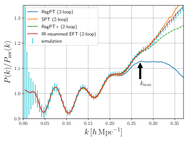
Figure 1: Predictions of power spectrum for each analytical method with fiducial cosmological parameters. For RegPT+ and IR-resummed EFT models, nuisance parameters are determined by the least-squares method using power spectrum up to $k_{\mathrm{max}}=0.27\,h\,\mathrm{Mpc}^{-1}$. The arrow shows the maximum wavenumber in the least-squares method. Note that spectra with these two models for wavenumbers larger than $k_{\mathrm{max}}$ are shown as dashed lines.

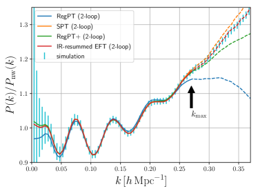
Figure 2: Power spectra with each analytical method with best-fit parameters with $k_{\mathrm{max}}=0.27\,h\,\mathrm{Mpc}^{-1}$. Note that spectra for wavenumbers larger than $k_{\mathrm{max}}$ are shown as dashed lines and the arrow shows $k_{\mathrm{max}}$. The best-fit cosmological parameters and nuisance parameters are estimated from MCMC chains.

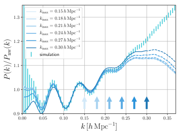
Figure 3: Best-fitting power spectra for RegPT at 2-loop level with best-fit parameters with different maximum wavenumbers from $0.15\,h\,\mathrm{Mpc}^{-1}$ to $0.30\,h\,\mathrm{Mpc}^{-1}$. The arrows show corresponding maximum wavenumbers $k_{\mathrm{max}}$. Note that spectra for wavenumbers larger than $k_{\mathrm{max}}$ are shown as dashed lines. The best-fit cosmological parameters are estimated from MCMC chains.

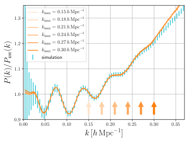
Figure 4: Best-fitting power spectra for SPT at 2-loop level with best-fit parameters with different maximum wavenumbers from $0.15\,h\,\mathrm{Mpc}^{-1}$ to $0.30\,h\,\mathrm{Mpc}^{-1}$. The arrows show corresponding maximum wavenumbers $k_{\mathrm{max}}$. Note that spectra for wavenumbers larger than $k_{\mathrm{max}}$ are shown as dashed lines. The best-fit cosmological parameters are estimated from MCMC chains.

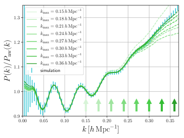
Figure 5: Best-fitting power spectra for RegPT+ at 2-loop level with best-fit parameters with different maximum wavenumbers from $0.15\,h\,\mathrm{Mpc}^{-1}$ to $0.36\,h\,\mathrm{Mpc}^{-1}$. The arrows show corresponding maximum wavenumbers $k_{\mathrm{max}}$. Note that spectra for wavenumbers larger than $k_{\mathrm{max}}$ are shown as dashed lines. The best-fit cosmological parameters are estimated from MCMC chains.

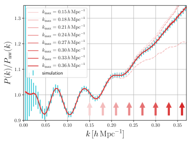
Figure 6: Best-fitting power spectra for IR-resummed EFT at 2-loop level with best-fit parameters with different maximum wavenumbers from $0.15\,h\,\mathrm{Mpc}^{-1}$ to $0.36\,h\,\mathrm{Mpc}^{-1}$. The arrows show corresponding maximum wavenumbers $k_{\mathrm{max}}$. Note that spectra for wavenumbers larger than $k_{\mathrm{max}}$ are shown as dashed lines. The best-fit cosmological parameters are estimated from MCMC chains.

IV.2 Parameter estimation with MCMC analysis

In Figs. 7, 8, 9, 10, and 11, the confidence regions of cosmological parameters with RegPT, SPT, RegPT+, and IR-resummed EFT at 2-loop level and RESPRESSO for $k_{\mathrm{max}}=0.21\,h\,\mathrm{Mpc}^{-1}$ are shown. At this scale, all prescriptions give the precise predictions of power spectrum and we can safely recover the input cosmological parameters. However, for example, the constraints with RegPT are tighter than those with IR-resummed EFT because free parameters introduced in this model degrade the resultant constraints. In addition, these parameters also affect parameter degeneracy between cosmological parameters. This effect will be addressed later in Sec. IV.5. For other models which contain no nuisance parameters, i.e., SPT and RESPRESSO, the constraints are almost the same as those with RegPT. On the other hand, for RegPT+, the constraints are weaker than those with RegPT as this model also introduces a free parameter.

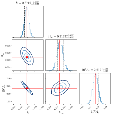
Figure 7: Parameter confidence regions with RegPT at 2-loop level and $k_{\mathrm{max}}=0.21\,h\,\mathrm{Mpc}^{-1}$. The light, normal, and dark blue lines correspond to the $1\text{-}\sigma$, $2\text{-}\sigma$, and $3\text{-}\sigma$ limits, respectively. The median and 16% and 84% percentiles are also shown on the top of each histogram. The black dashed lines correspond to 16% and 84% percentiles. The red lines show the input parameters.

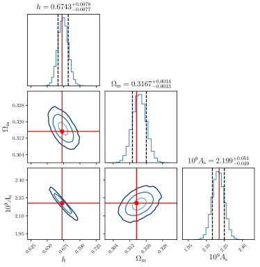
Figure 8: Parameter confidence regions with SPT at 2-loop level and $k_{\mathrm{max}}=0.21\,h\,\mathrm{Mpc}^{-1}$. The light, normal, and dark blue lines correspond to the $1\text{-}\sigma$, $2\text{-}\sigma$, and $3\text{-}\sigma$ limits, respectively. The median and 16% and 84% percentiles are also shown on the top of each histogram. The black dashed lines correspond to 16% and 84% percentiles. The red lines show the input parameters.

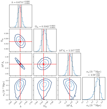
Figure 9: Parameter confidence regions with RegPT+ at 2-loop level and $k_{\mathrm{max}}=0.21\,h\,\mathrm{Mpc}^{-1}$. The light, normal, and dark blue lines correspond to the $1\text{-}\sigma$, $2\text{-}\sigma$, and $3\text{-}\sigma$ limits, respectively. The median and 16% and 84% percentiles are also shown on the top of each histogram. The black dashed lines correspond to 16% and 84% percentiles. The red lines show the input parameters.

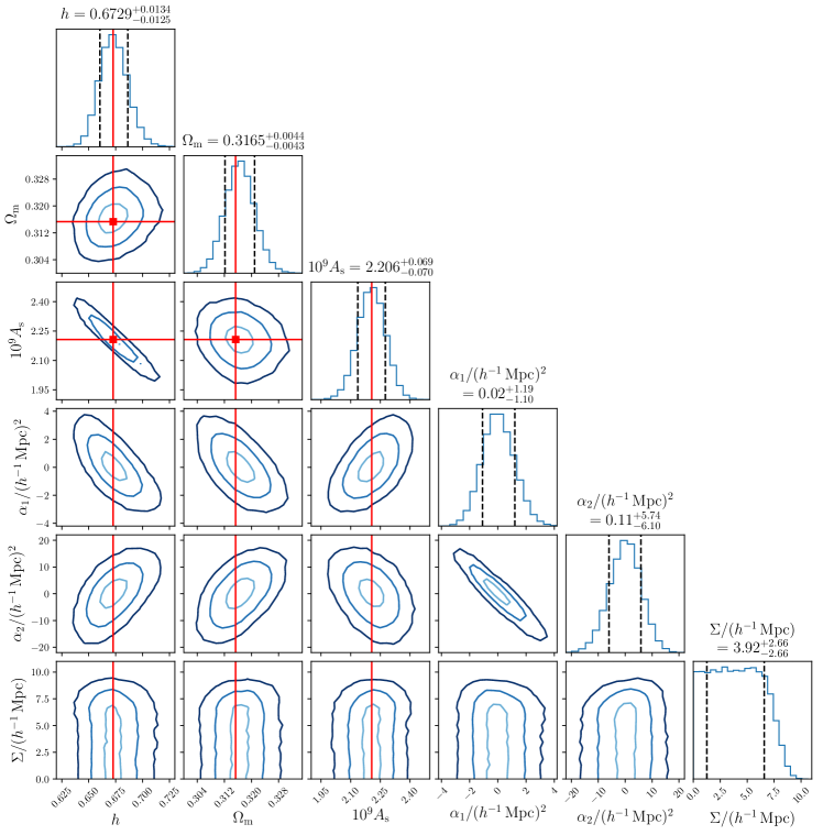
Figure 10: Parameter confidence regions with IR-resummed EFT at 2-loop level and $k_{\mathrm{max}}=0.21\,h\,\mathrm{Mpc}^{-1}$. The light, normal, and dark blue lines correspond to the $1\text{-}\sigma$, $2\text{-}\sigma$, and $3\text{-}\sigma$ limits, respectively. The median and 16% and 84% percentiles are also shown on the top of each histogram. The black dashed lines correspond to 16% and 84% percentiles. The red lines show the input parameters.

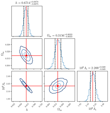
Figure 11: Parameter confidence regions with RESPRESSO at 2-loop level and $k_{\mathrm{max}}=0.21\,h\,\mathrm{Mpc}^{-1}$. The light, normal, and dark blue lines correspond to the $1\text{-}\sigma$, $2\text{-}\sigma$, and $3\text{-}\sigma$ limits, respectively. The median and 16% and 84% percentiles are also shown on the top of each histogram. The black dashed lines correspond to 16% and 84% percentiles. The red lines show the input parameters.

Next, we show the estimated cosmological and nuisance parameters with analytical models at 2-loop level in Figs. 12 and 13. The values plotted in these figures are medians, which are robust to outliers, instead of means. However, for cosmological parameters, since the posterior distributions are symmetric, the median and mean are almost the same. On the other hand, for some of nuisance parameters (see, e.g., the parameter $\Sigma$ in Fig. 10), the posterior distribution is far from symmetric, the median can be different from the sample mean. The range of error bars corresponds to 16% and 84% percentiles, which correspond to $1\text{-}\sigma$ range when the posterior distribution is completely Gaussian. For RegPT at 2-loop level, this model gives unbiased estimates up to $k_{\mathrm{max}}\lesssim 0.24\,h\,\mathrm{Mpc}^{-1}$, where the calculations are supposed to be accurate. As a general trend, the errors become small by increasing $k_{\mathrm{max}}$ because more information become available. However, at high $k\gtrsim 0.25\,h\,\mathrm{Mpc}^{-1}$, this model is not supposed to compute the spectrum accurately (see Fig. 1). As a result, the fitting process itself breaks down, and then errors increase and estimated parameters deviate from the true values. RegPT+, IR-resummed EFT, and RESPRESSO can all reproduce the input cosmological parameters up to high $k_{\mathrm{max}}$. However, RegPT+ and IR-resummed EFT contain free nuisance parameters and thus they have more degrees of freedom to fit the power spectrum. Thus, that leads to degradation of constraints.

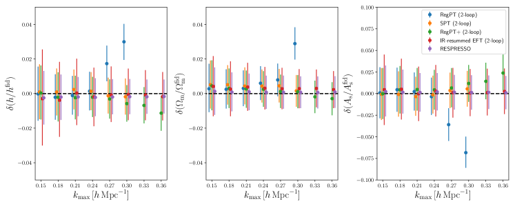
Figure 12: Medians of cosmological parameters estimated from MCMC chains with errors, shown as the fractional ratios with respect to the fiducial values. The lower (upper) limit of error bars correspond to $16\%$ ($84\%$) percentile.

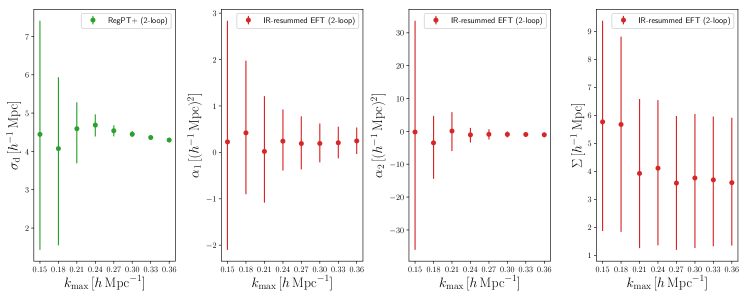
Figure 13: Medians of nuisance parameters, $\sigma_{\mathrm{d}}$ for RegPT+ and $\alpha_{1}$, $\alpha_{2}$, and $\Sigma$ for IR-resummed EFT, estimated from MCMC chains. The lower (upper) limit of error bars correspond to $16\%$ ($84\%$) percentile.

IV.3 Figure of bias

Here, we quantify how close to the input cosmological parameters estimated parameters are for each template with respect to the statistical errors. For this purpose, first we compute the correlation matrix of all parameters $S$, i.e., cosmological parameters and nuisance parameters ($\sigma_{\mathrm{d}}$ for RegPT+ and $\alpha_{1}$, $\alpha_{2}$, and $\Sigma$ for IR-resummed EFT), which can be estimated from MCMC chains:

$$S_{\alpha\beta}=\frac{1}{N-1}\sum_{k}^{N}(\theta_{\alpha}^{k}-\bar{\theta}_{\alpha})(\theta_{\beta}^{k}-\bar{\theta}_{\beta}),$$ (24)

where $\bm{\theta}^{k}$ is a parameter vector at the $k$-th step, $N$ is the number of total steps in chains, and $\bar{\bm{\theta}}$ is the sample mean of the parameters. We are interested only in cosmological parameters and marginalize the posterior distribution over the nuisance parameters. Under the assumption that the parameters follow the multivariate Gaussian distribution, this operation simply corresponds to taking submatrix, which is denoted by $\tilde{S}$. Then, we define the figure of bias (FoB) as,

$$\mathrm{FoB}\equiv\left[\sum_{\alpha,\beta}\delta\theta_{\alpha}\left(\tilde{S}\right)^{-1}_{\alpha\beta}\delta\theta_{\beta}\right]^{1/2},$$ (25)

where $\delta\bm{\theta}$ is the difference between the estimated and input cosmological parameters Taruya et al. (2011). FoB corresponds to the distance between true and estimated cosmological parameters normalized by their variances. In Fig. 14, we show FoBs with different models and $k_{\mathrm{max}}$ along with $1\text{-}\sigma$, $2\text{-}\sigma$, and $3\text{-}\sigma$ critical values, which correspond to $68\%$, $95\%$, and $99.7\%$ percentiles, respectively, in the case of three parameters, when the parameter deviation $\delta\bm{\theta}$ follows multivariate Gaussian. These critical values are derived from cumulative distribution function for the chi-squared distribution. The degree of freedom is 3 regardless of the choice of the model because the nuisance parameters have already been marginalized. FoBs of SPT and RegPT exceed the $1\text{-}\sigma$ critical value from relatively small $k_{\mathrm{max}}$ while FoBs of RegPT+ and IR-resummed EFT are kept small even for high $k_{\mathrm{max}}$. This fact means that we can employ RegPT+ and IR-resummed EFT up to scales $\gtrsim 0.30\,h\,\mathrm{Mpc}^{-1}$ without having a substantial biased parameter estimation. However, there is a caveat about the small FoBs. Since FoB is normalized by the variance of parameters, if power of constraining parameters is weak, the resultant FoB will be also small. In the cases of RegPT+ and IR-resummed EFT, the nuisance parameters degrade constraints and that leads to large variances. Though these models can provide us with the accurate prediction even at small scales, their small FoBs should be taken with cautions. The FoB of RESPRESSO is not shown in Fig. 14 because, as stated before, the simulations used in the analysis is also used to calibrate the response function in RESPRESSO and thus the FoB of RESPRESSO should always be zero.

So far, we have presented FoBs with power spectra at 2-loop level, but as a whole, those with spectra at 1-loop level show similar behavior qualitatively. However, FoBs are generally larger and exceed $1\text{-}\sigma$ limit even for smaller $k_{\mathrm{max}}$. We present detailed discussions for results at 1-loop level in Appendix B.

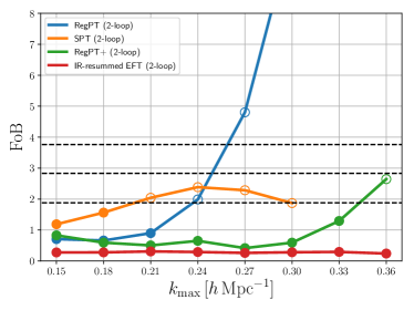
Figure 14: Figure of bias for different models estimated from MCMC chains. The black dashed lines show the $1\text{-}\sigma$, $2\text{-}\sigma$, and $3\text{-}\sigma$ critical values $1.88$, $2.83$, and $3.76$, respectively. The open (filled) symbols represent that the figure of bias exceeds (falls below) the $1\text{-}\sigma$ critical value.

IV.4 Figure of merit

Next, we quantify the precision of parameter estimation for each model using figure of merit (FoM). We define FoM as the inverse of volume of the parameter space determined by iso-posterior density surface Albrecht et al. (2006), i.e.,

$$\mathrm{FoM}\equiv\frac{1}{\sqrt{\mathrm{det}\tilde{S}}}.$$ (26)

Roughly speaking, FoM is an indicator of constraining power for each model. We also introduce an analytical way to estimate the upper limit of FoM for RESPRESSO. With response function approach, we can compute the Fisher information matrix. Since the covariance matrix does not depend on parameters, the Fisher matrix can be given as

$$F_{\alpha\beta}=\sum_{k_{i},k_{j}<k_{\mathrm{max}}}\frac{\partial P(k_{i})}{\partial\theta_{\alpha}}(C^{-1})_{ij}\frac{\partial P(k_{j})}{\partial\theta_{\beta}}.$$ (27)

The derivatives of the power spectrum can be obtained via the response function (Eq. 22),

$$\frac{\partial P(k)}{\partial\theta_{\alpha}}=\int dq\frac{\delta P(k)}{\delta P_{\mathrm{L}}(q)}\frac{\partial P_{\mathrm{L}}(q)}{\partial\theta_{\alpha}}=\int d\ln q\,K(k,q)\frac{\partial P_{\mathrm{L}}(q)}{\partial\theta_{\alpha}}.$$ (28)

Then the Fisher matrix estimate of the FoM is given by,

$$\mathrm{FoM}_{F}=\sqrt{\det F}.$$ (29)

From the Cramér-Rao bound Albrecht et al. (2009), FoMs for RESPRESSO can not exceed $\mathrm{FoM}_{F}$. If the likelihood distribution (Eq. 20) follows Gaussian with respect to parameters, $\mathrm{FoM}_{F}$ coincides with FoM computed from correlation matrix (Eq. 26).

In Fig. 15, we show FoMs with different models and $k_{\mathrm{max}}$ and Fisher matrix approach with RESPRESSO. Generally, FoM increases with $k_{\mathrm{max}}$ because more information becomes available. As a whole, RegPT, SPT, and RESPRESSO work quite well. However, shown in Fig. 14, FoBs of RegPT and SPT soon exceed the $1\text{-}\sigma$ limit leading to biased estimated parameters. On the other hand, FoMs of RegPT+ and IR-resummed EFT are significantly suppressed with respect to RESPRESSO results. Clearly though free parameters contained in these models help to fit the power spectra down to small scales, the presence of extra degrees of freedom degrades the constraining power of these models.

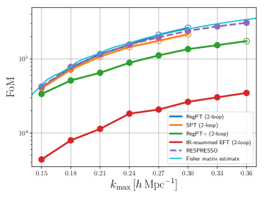
Figure 15: Figure of merit for different models estimated from MCMC chains. The result with RESPRESSO is shown as a dashed line since it is different from other methods in the sense that it relies on simulation-aided approach, not completely analytical prescription. The cyan line shows figure of merit from Fisher matrix with RESPRESSO. The open (filled) symbols represent that the corresponding figure of bias exceeds (falls below) the $1\text{-}\sigma$ critical value (see Fig. 14).

IV.5 Correlations between parameters

Generally, nuisance parameters help to improve fitting power spectrum even at small scales. Simultaneously, if cosmological parameters are taken far from the true value, nuisance parameters can adjust spectra and thus constraints on cosmological parameters will be degraded. This effect can be observed in the parameter degeneracy between cosmological and nuisance parameters. The degeneracy means that the effect due to the cosmological parameter can be compensated by changing the nuisance parameter. On the other hand, when there is no degeneracy, the nuisance parameter simply enhances the prediction capability of the model or has almost no effects in the interested ranges. In order to address this effect, we quantify the degeneracy between parameters from correlation coefficients defined as,

$$R_{\alpha\beta}\equiv\frac{S_{\alpha\beta}}{\sqrt{S_{\alpha\alpha}S_{\beta\beta}}}.$$ (30)

In Figs. 16, 17, 18, 19, and 20, the correation coefficients for all pairs of parameters with RegPT, SPT, RegPT+, IR-resummed EFT, and RESPRESSO for $k_{\mathrm{max}}=0.18,\,0.24\,h\,\mathrm{Mpc}^{-1}$ are shown. We observe that changing $k_{\mathrm{max}}$ does not alter significantly the structure of the correlation matrix. However, if $k_{\mathrm{max}}$ is higher than the scale where each model is reliable or equivalently the corresponding FoB is high, the correlations might be altered. In RegPT+ model, the nuisance parameter $\sigma_{\mathrm{d}}$ is moderately degenerate with cosmological parameters, and for IR-resummed EFT model, the parameters $\alpha_{1}$ and $\alpha_{2}$ are strongly correlated with cosmological parameters though the parameter $\Sigma$ does not show strong correlation. This degeneracy reduces the constraining power and leads to the suppression of FoM. Since there exists stronger degeneracy in IR-resummed EFT model, the suppression of FoM is more appreciable. The parameter degeneracy also changes the degeneracy between cosmological parameters, and the resultant correlation becomes different from no nuisance parameter case via marginalization (see Figs. 16 and 17 in the cases of RegPT and SPT, respectively).

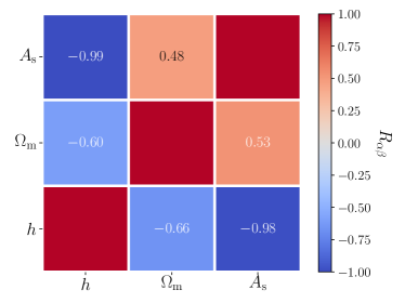
Figure 16: Correlation coefficients for RegPT at 2-loop level. The upper left (lower right) triangle shows results with $k_{\mathrm{max}}=0.18\,(0.24)\,h\,\mathrm{Mpc}^{-1}$. The red (blue) parts correspond to positive (negative) correlations.

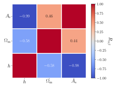
Figure 17: Correlation coefficients for SPT at 2-loop level. The upper left (lower right) triangle shows results with $k_{\mathrm{max}}=0.18\,(0.24)\,h\,\mathrm{Mpc}^{-1}$. The red (blue) parts correspond to positive (negative) correlations.

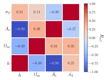
Figure 18: Correlation coefficients for RegPT+ at 2-loop level. The upper left (lower right) triangle shows results with $k_{\mathrm{max}}=0.18\,(0.24)\,h\,\mathrm{Mpc}^{-1}$. The red (blue) parts correspond to positive (negative) correlations.

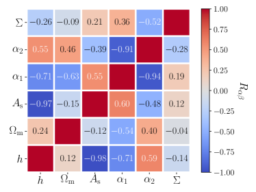
Figure 19: Correlation coefficients for IR-resummed EFT at 2-loop level. The upper left (lower right) triangle shows results with $k_{\mathrm{max}}=0.18\,(0.24)\,h\,\mathrm{Mpc}^{-1}$. The red (blue) parts correspond to positive (negative) correlations.

Figure 20: Correlation coefficients for RESPRESSO. The upper left (lower right) triangle shows results with $k_{\mathrm{max}}=0.18\,(0.24)\,h\,\mathrm{Mpc}^{-1}$. The red (blue) parts correspond to positive (negative) correlations.

V Conclusions

The measurement of matter power spectrum or the BAO feature imprinted on it has been considered to be one of the most fundamental observables in precision cosmology. But in order to efficiently constrain cosmological models or parameters, observables such as power spectrum should be analytically modeled beyond the linear theory. In this work, we explore the efficiency with which such models could constrain the cosmological parameters focusing our analysis on what could be derived from real space power spectrum. The latter is obtained from an $N$-body simulation for a specific set of cosmological parameters. The performances of analytical models can then be scrutinized in terms of precision and accuracy.

The analytical approaches we employ are

• Standard Perturbation Theory, (SPT), based on a direct expansion of the Euler fluid equations with respect to linear density contrast;

• Regularized Perturbation Theory, (RegPT), based on a reorganization of the series expansion with the help of the multipoint propagators;

• An extension of RegPT (RegPT+) in which the damping scale is taken as a free parameter to account for the fact that it not predictable from first principle calculations;

• An IR-resummed Effective Field Theory (EFT) model in which non-PT parameters are introduced to account for the impact of the small scale physics on the growth of spectra, such as the effective pressure, etc.

Those models, all considered up to 2-loop order, are more precisely described in Sec. II. Our whole procedure is checked and calibrated with the help of RESPRESSO which can accurately predict how nonlinear power spectrum are deformed, in the whole range of modes of interest, when the cosmological parameters are varied. Taking advantage of a simulated mock observation of real space power spectrum, cosmological parameters are then fitted using the analytical models described above with the MCMC technique.

In order to precisely quantify the performances of the codes we used the Figure of Bias (FoB), which is the difference between estimated and input parameters normalized by the variances, and the Figure of Merit (FoM), which roughly corresponds to the inverse of the volume of the confidence region. Our findings from the analysis with power spectrum at the redshift $z=1$ can be summarized as follows,

• RegPT and SPT give unbiased estimates of the cosmological parameters when the range of modes used to fit the parameters is limited to $k_{\mathrm{max}}=0.24\,h\,\mathrm{Mpc}^{-1}$. They fail for higher $k_{\mathrm{max}}$. RegPT+ and IR-resummed EFT are accurate up to $k_{\mathrm{max}}=0.30\,h\,\mathrm{Mpc}^{-1}$ thanks to the extra degrees of freedom they contain.

• On the other hand, as expected, FoMs of a given model monotonically increase as a function of $k_{\mathrm{max}}$ as the amount of available information increases. And as expected the resulting precision in the cosmological parameters is all the more sensitive to $k_{\mathrm{max}}$ that the number of useful modes scales like $k_{\mathrm{max}}^{3}$.

• FoMs of models with extra free parameters, RegPT+ and IR-resummed EFT, are significantly reduced, by a factor respectively about 2 and 10, compared with those from models that are entirely predictive such as SPT and RegPT in our case. This effect is roughly independent of $k_{\mathrm{max}}$.

In order to address more precisely the origin of the latter reduction, we investigate how nuisance parameters correlate with cosmological parameters taking advantage of the fact that such correlation coefficients can be coherently extracted from the MCMC chains. Our results are presented in Sec. IV.5. We find that some of the nuisance parameters are degenerate with cosmological parameters degrading the precision with which the latter are determined. This effect is all the more important that the number of free parameters is large. It is on the other hand quite independent of $k_{\mathrm{max}}$. We are then put in a situation where a trade-off should be found between accuracy, which calls for more free parameters, and precision, which calls for less. The best performing prescription of those we consider here is the RegPT+ model, having only one free nuisance parameter while still being able to provide unbiased estimates up to $k_{\mathrm{max}}$ about $0.33\,h\,\mathrm{Mpc}^{-1}$. This is unlikely however to be a definitive results: other prescriptions could probably be as effective and this validity range depends in effect on the detailed covariance properties of the mock data.

Note that in this exercise, we were forced to restrict the chains to a three dimensional cosmological parameter space (six dimensional space in total for EFT models). The reason is that the code we used here was not fast enough to cope with larger dimensional space . Needless is to say that the larger the number of parameters is, the slower the convergence of the MCMC procedure is. For exploring larger parameter spaces, it is then crucial to implement fast methods for computing power spectrum. Several methods have already been proposed to speed up 2-loop level calculations Schmittfull et al. (2016); Schmittfull and Vlah (2016); Simonović et al. (2018). Other aspects which should eventually be incorporated are modified gravity, which is addressed in the context of EFT in Ref. Bose et al. (2018), galaxy bias, and redshift space distortions effects. They also lead to a further increase of the number of parameters to use. These will be subjects of subsequent papers.

We are planning to release a set of numerical codes to compute the power spectrum perturbatively based on the fast scheme originally proposed by Ref. Taruya et al. (2012). The code suite will handle redshift space distortions and galaxy bias with the fast scheme consistently up to the 2-loop level. We have made an initial version of this code available on the repository (https://github.com/0satoken/Eclairs). The current version supports computation of matter power spectrum in real space based on analytical approaches presented in this paper. The codes are written in C++ with the python wrapper, which is designed to be easily combined with MCMC samplers.

Appendix A Explicit formulas of analytical approaches

In this Appendix, we present explicit formulas for power spectrum based on SPT, RegPT, and IR-resummed EFT.

A.1 SPT

The correction terms of power spectrum based on SPT at 1-loop and 2-loop levels are

$$\Delta P^{\text{SPT}}_{\text{1-loop}}(k) = D_{+}^{4}[2P_{13}(k)+P_{22}(k)],$$ (31)

$$\Delta P^{\text{SPT}}_{\text{2-loop}}(k) = D_{+}^{6}[2P_{15}(k)+2P_{24}(k)+P_{33}(k)].$$ (32)

Each correction term is given as

$$P_{13}(k) = 3P_{0}(k)\int\frac{d^{3}q}{(2\pi)^{3}}F_{\mathrm{sym}}^{(3)}(\bm{k},\bm{q},-\bm{q})P_{0}(q),$$ (33)

$$P_{22}(k) = 2\int\frac{d^{3}q}{(2\pi)^{3}}[F_{\mathrm{sym}}^{(2)}(\bm{q},\bm{k}-\bm{q})]^{2}P_{0}(q)P_{0}(|\bm{k}-\bm{q}|),$$ (34)

$$P_{15}(k) = 15P_{0}(k)\int\frac{d^{3}q_{1}}{(2\pi)^{3}}\frac{d^{3}q_{2}}{(2\pi)^{3}}F_{\mathrm{sym}}^{(5)}(\bm{k},\bm{q}_{1},-\bm{q}_{1},\bm{q}_{2},-\bm{q}_{2})P_{0}(q_{1})P_{0}(q_{2}),$$ (35)

$$P_{24}(k) = 12\int\frac{d^{3}q_{1}}{(2\pi)^{3}}\frac{d^{3}q_{2}}{(2\pi)^{3}}F_{\mathrm{sym}}^{(2)}(\bm{q}_{1},\bm{k}-\bm{q}_{1})F_{\mathrm{sym}}^{(4)}(\bm{q}_{1},\bm{k}-\bm{q}_{1},\bm{q}_{2},-\bm{q}_{2})P_{0}(q_{1})P_{0}(q_{2})P_{0}(|\bm{k}-\bm{q}_{1}|),$$ (36)

$$P_{33}(k) = 9P_{0}(k)\left[\int\frac{d^{3}q}{(2\pi)^{3}}F_{\mathrm{sym}}^{(3)}(\bm{k},\bm{q},-\bm{q})P_{0}(q)\right]^{2}$$ (37)

$$+6\int\frac{d^{3}q_{1}}{(2\pi)^{3}}\frac{d^{3}q_{2}}{(2\pi)^{3}}[F_{\mathrm{sym}}^{(3)}(\bm{q}_{1},\bm{q}_{2},\bm{k}-\bm{q}_{1}-\bm{q}_{2})]^{2}P_{0}(q_{1})P_{0}(q_{2})P_{0}(|\bm{k}-\bm{q}_{1}-\bm{q}_{2}|).$$

Eventually, the power spectra at 1-loop and 2-loop levels are given as

$$P^{\text{SPT}}_{\text{1-loop}}(k) = P_{\mathrm{L}}(k)+\Delta P^{\text{SPT}}_{\text{1-loop}}(k),$$ (38)

$$P^{\text{SPT}}_{\text{2-loop}}(k) = P_{\mathrm{L}}(k)+\Delta P^{\text{SPT}}_{\text{1-loop}}(k)+\Delta P^{\text{SPT}}_{\text{2-loop}}(k).$$ (39)

A.2 RegPT

The expression of power spectrum of RegPT at 2-loop level should be

$$P^{\texttt{RegPT}}_{\text{2-loop}}(k) = [\Gamma_{\mathrm{reg}}^{(1)}(k)]^{2}P_{0}(k)+2\int\frac{d^{3}q}{(2\pi)^{3}}[\Gamma_{\mathrm{reg}}^{(2)}(\bm{q},\bm{k}-\bm{q})]^{2}P_{0}(q)P_{0}(|\bm{k}-\bm{q}|)$$ (40)

$$+6\int\frac{d^{3}q_{1}}{(2\pi)^{3}}\frac{d^{3}q_{2}}{(2\pi)^{3}}[\Gamma_{\mathrm{reg}}^{(3)}(\bm{q}_{1},\bm{q}_{2},\bm{k}-\bm{q}_{1}-\bm{q}_{2})]^{2}P_{0}(q_{1})P_{0}(q_{2})P_{0}(|\bm{k}-\bm{q}_{1}-\bm{q}_{2}|),$$

where the regularized propagators are expressed as,

$$\Gamma^{(1)}_{\mathrm{reg}}(k) = D_{+}\left[1+\alpha_{k}+\frac{1}{2}\alpha_{k}^{2}\right.$$ (41)

$$\left.+D_{+}^{2}\Gamma^{(1)}_{\text{1-loop}}(k)(1+\alpha_{k})+D_{+}^{4}\Gamma^{(1)}_{\text{2-loop}}(k)\right]$$

$$\times\exp(-\alpha_{k}),$$

$$\Gamma^{(2)}_{\mathrm{reg}}(\bm{k}_{1},\bm{k}_{2}) = D_{+}^{2}\left[(1+\alpha_{k})F^{(2)}_{\mathrm{sym}}(\bm{k}_{1},\bm{k}_{2})\right.$$ (42)

$$\left.+D_{+}^{2}\Gamma^{(2)}_{\text{1-loop}}(\bm{k}_{1},\bm{k}_{2})\right]\exp(-\alpha_{k}),$$

$$\Gamma^{(3)}_{\mathrm{reg}}(\bm{k}_{1},\bm{k}_{2},\bm{k}_{3}) = D_{+}^{3}F^{(3)}_{\mathrm{sym}}(\bm{k}_{1},\bm{k}_{2},\bm{k}_{3})\exp(-\alpha_{k}),$$ (43)

where $\alpha_{k}=(1/2)k^{2}D_{+}^{2}\sigma_{\mathrm{d}}^{2}$, and $\Gamma^{(1)}_{\text{1-loop}}(k)$, $\Gamma^{(1)}_{\text{2-loop}}(k)$, and $\Gamma^{(2)}_{\text{1-loop}}(\bm{k}_{1},\bm{k}_{2})$ are defined in Eq. (8).

The power spectrum at 1-loop level is given as

$$P^{\texttt{RegPT}}_{\text{1-loop}}(k) = [\Gamma_{\mathrm{reg}}^{(1)}(k)]^{2}P_{0}(k)$$

$$+2\int\frac{d^{3}q}{(2\pi)^{3}}[\Gamma_{\mathrm{reg}}^{(2)}(\bm{q},\bm{k}-\bm{q})]^{2}P_{0}(q)P_{0}(|\bm{k}-\bm{q}|),$$

with the corresponding regularized propagators $\Gamma^{(1)}_{\mathrm{reg}}$ and $\Gamma^{(2)}_{\mathrm{reg}}$,

$$\Gamma^{(1)}_{\mathrm{reg}}(k) = D_{+}\left[1+\alpha_{k}+D_{+}^{2}\Gamma^{(1)}_{\text{1-loop}}(k)\right]$$ (45)

$$\times\exp(-\alpha_{k}),$$

$$\Gamma^{(2)}_{\mathrm{reg}}(\bm{k}_{1},\bm{k}_{2}) = D_{+}^{2}F^{(2)}_{\mathrm{sym}}(\bm{k}_{1},\bm{k}_{2})\exp(-\alpha_{k}).$$ (46)

A.3 IR-resummed EFT

In the following, we give expressions for matter power spectrum at 2-loop and 1-loop levels based on the IR-resummed EFT approach. At 2-loop level, the matter power spectrum is given as,

$$P^{\text{IR EFT}}_{\text{2-loop}}(k) = P^{\mathrm{nw}}(k)+P^{\mathrm{w}}(k);$$ (47)

$$P^{\mathrm{nw}}(k) = (1+\alpha_{1}k^{2})P_{\mathrm{L}}^{\mathrm{nw}}(k)+(1+\alpha_{2}k^{2})\Delta P_{\text{1-loop}}^{\mathrm{nw}}(k)+\Delta P^{\mathrm{nw}}_{\text{2-loop}}(k),$$ (48)

$$P^{\mathrm{w}}(k) = e^{-k^{2}\Sigma^{2}}\left[(1+\alpha_{1}k^{2}+C_{1})P_{\mathrm{L}}^{\mathrm{w}}(k)+(1+\alpha_{2}k^{2}+C_{2})\Delta P_{\text{1-loop}}^{\mathrm{w}}(k)+\Delta P_{\text{2-loop}}^{\mathrm{w}}(k)\right],$$ (49)

where

$$C_{1} = k^{2}\Sigma^{2}(1+\alpha_{1}k^{2})+\frac{1}{2}k^{4}\Sigma^{4},$$ (50)

$$C_{2} = k^{2}\Sigma^{2}(1+\alpha_{2}k^{2}).$$ (51)

Here, we have introduced three free parameters $\alpha_{1}$, $\alpha_{2}$, and $\Sigma$, which are usually calibrated with $N$-body simulations. For no-wiggle linear spectra $P_{\mathrm{L}}^{\mathrm{nw}}(k)$, we smooth linear power spectrum as described in Eqs. (13) and (14), i.e.,

$$P_{\mathrm{L}}^{\mathrm{nw}}(k) = P_{\mathrm{EH}}(k)\frac{1}{\sqrt{2\pi}\log_{10}\lambda}\int d(\log_{10}q)\frac{P_{\mathrm{L}}(q)}{P_{\mathrm{EH}}(q)}$$ (52)

$$\times\exp\left[-\frac{(\log_{10}k-\log_{10}q)^{2}}{2(\log_{10}\lambda)^{2}}\right],$$

where we adopt the smoothing scale as $\lambda=10^{0.25}\,h\,\mathrm{Mpc}^{-1}$ and $P_{\mathrm{EH}}(k)$ is the power spectrum without wiggle feature Eisenstein and Hu (1998). The residual corresponds to the wiggle part $P_{\mathrm{L}}^{\mathrm{w}}(k)$, i.e.,

$$P_{\mathrm{L}}^{\mathrm{w}}(k)=P_{\mathrm{L}}(k)-P_{\mathrm{L}}^{\mathrm{nw}}(k).$$ (53)

Then, we plug the smoothed spectrum $P_{\mathrm{L}}^{\mathrm{nw}}(k)$, instead of linear spectrum $P_{\mathrm{L}}(k)$, into the SPT formulas (Eqs. 31 and 32) to obtain no-wiggle correction terms at 1-loop and 2-loop levels ($\Delta P_{\text{1-loop}}^{\mathrm{nw}}$ and $\Delta P_{\text{2-loop}}^{\mathrm{nw}}$). The wiggle parts of correction terms are also obtained as residuals,

$$\Delta P_{\text{1-loop}}^{\mathrm{w}}(k) = \Delta P^{\text{SPT}}_{\text{1-loop}}(k)-\Delta P_{\text{1-loop}}^{\mathrm{nw}}(k),$$ (54)

$$\Delta P_{\text{2-loop}}^{\mathrm{w}}(k) = \Delta P^{\text{SPT}}_{\text{2-loop}}(k)-\Delta P_{\text{2-loop}}^{\mathrm{nw}}(k).$$ (55)

For 1-loop level, the matter power spectrum is given as,

$$P^{\text{IR EFT}}_{\text{1-loop}}(k) = P^{\mathrm{nw}}(k)+P^{\mathrm{w}}(k),$$ (56)

$$P^{\mathrm{nw}}(k) = (1+\alpha_{1}k^{2})P_{\mathrm{L}}^{\mathrm{nw}}(k)+\Delta P_{\text{1-loop}}^{\mathrm{nw}}(k),$$

$$P^{\mathrm{w}}(k) = e^{-k^{2}\Sigma^{2}}\left[(1+\alpha_{1}k^{2}+k^{2}\Sigma^{2})P_{\mathrm{L}}^{\mathrm{w}}(k)\right.$$ (58)

$$\left.+\Delta P_{\text{1-loop}}^{\mathrm{w}}(k)\right].$$

In this case, there are two free parameters, $\alpha_{1}$ and $\Sigma$, which are also calibrated against $N$-body simulations.

A.4 EFT

We have considered IR-resummed EFT so far but there is a simpler description of EFT. For 1-loop level, we can write down the expression for EFT as,

$$P^{\text{EFT}}_{\text{1-loop}}(k)=P^{\text{SPT}}_{\text{1-loop}}(k)-2(2\pi)c_{s(1)}^{2}\left(\frac{k}{k_{\mathrm{NL}}}\right)^{2}P_{\mathrm{L}}(k),$$ (59)

where $k_{\mathrm{NL}}$ is the nonlinear scale and $c_{s(1)}$ is the effective sound speed Carrasco et al. (2014). We treat the combination $c_{s(1)}/k_{\mathrm{NL}}$ as a free parameter. The EFT prescription is based on the similar idea for IR-resummed EFT, and roughly speaking the parameter $\alpha_{1}$ in IR-resummed EFT corresponds to the sound speed in EFT. Thus, these two models should provide us with similar results. However, IR-resummed EFT introduces another free parameter $\Sigma$ which regulates the damping feature at small scales and when $\Sigma=0$, the expression can be reduced to that of EFT.

Appendix B Results with power spectra at 1-loop level

For comparison, we present results with methods at 1-loop level. In Figs. 21 and 22, cosmological and nuisance parameters estimated with 1-loop level calculations are shown. The results look mostly similar to 2-loop cases. However, the estimated parameters start to deviate from true values from smaller $k_{\mathrm{max}}$. We can see a similar trend in FoB and FoM shown in Figs. 23 and 24. According to FoM, the constraining power is almost the same as that at 2-loop level. On the other hand, in all cases FoBs are higher than the counterpart in the 2-loop case. The 2-loop level calculations outperform 1-loop calculations though they are computationally more expensive. The FoM of EFT is slightly larger than that of IR-resummed EFT but the effect is subdominant. In order to investigate the reason, we show correlation coefficients for IR-resummed EFT and EFT in Figs. 25 and 26. In IR-resummed EFT model, the parameter $\Sigma$ has almost no correlations with cosmological parameters. That results in no degradation of parameter constraints due to $\Sigma$. On the other hand, $\alpha_{1}$ in IR-resummed EFT and $c_{s(1)}/k_{\mathrm{NL}}$ in EFT correlates with cosmological parameters to similar extent, and thus FoMs for these two models are almost the same.

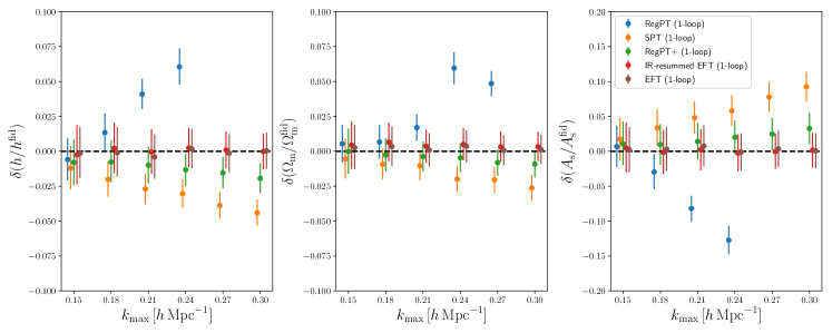
Figure 21: Medians of cosmological parameters estimated from MCMC chains with errors as the fractional ratios with respect to the fiducial values. All of estimates are based on 1-loop level calculations. The lower (upper) limit of error bars correspond to $16\%$ ($84\%$) percentile.

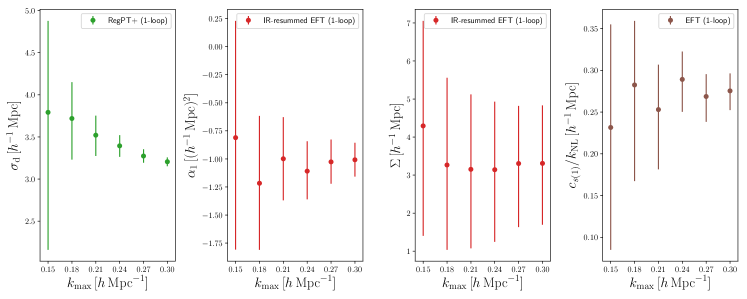
Figure 22: Medians of nuisance parameters, $\sigma_{\mathrm{d}}$ for RegPT+, $\alpha_{1}$ and $\Sigma$ for IR-resummed EFT, and $c_{s(1)}/k_{\mathrm{NL}}$ for EFT, estimated from MCMC chains. The lower (upper) limit of error bars correspond to $16\%$ ($84\%$) percentile.

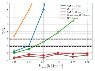
Figure 23: Figure of bias for different models at at 1-loop level estimated from MCMC chains. The black dashed line shows the $1\text{-}\sigma$, $2\text{-}\sigma$, and $3\text{-}\sigma$ critical values $1.88$, $2.83$, and $3.76$. The open (filled) symbols represent that the figure of bias exceeds (falls below) the $1\text{-}\sigma$ critical value.

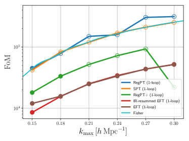
Figure 24: Figure of merit for different models at 1-loop level estimated from MCMC chains. The cyan line shows figure of merit from Fisher matrix with RESPRESSO. The open (filled) symbols represent that the corresponding figure of bias exceeds (falls below) the $1\text{-}\sigma$ critical value (see Fig. 23).

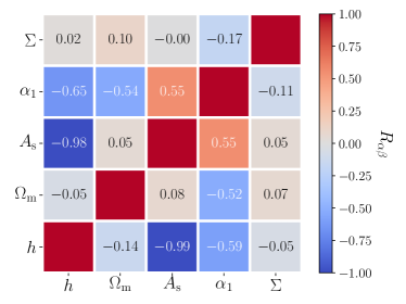
Figure 25: Correlation coefficients for IR-resummed EFT model at 1-loop level. The upper left (lower right) triangle shows results with $k_{\mathrm{max}}=0.18\,(0.24)\,h\,\mathrm{Mpc}^{-1}$. The red (blue) parts correspond to positive (negative) correlations.

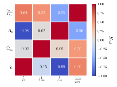
Figure 26: Correlation coefficients for EFT at 1-loop level. The upper left (lower right) triangle shows results with $k_{\mathrm{max}}=0.18\,(0.24)\,h\,\mathrm{Mpc}^{-1}$. The red (blue) parts correspond to positive (negative) correlations.

References

- Aubourg et al. (2015) É. Aubourg, S. Bailey, J. E. Bautista, F. Beutler, V. Bhardwaj, D. Bizyaev, M. Blanton, M. Blomqvist, A. S. Bolton, J. Bovy, H. Brewington, J. Brinkmann, J. R. Brownstein, A. Burden, N. G. Busca, W. Carithers, C.-H. Chuang, J. Comparat, R. A. C. Croft, A. J. Cuesta, K. S. Dawson, T. Delubac, D. J. Eisenstein, A. Font-Ribera, J. Ge, J.-M. Le Goff, S. G. A. Gontcho, J. R. Gott, J. E. Gunn, H. Guo, J. Guy, J.-C. Hamilton, S. Ho, K. Honscheid, C. Howlett, D. Kirkby, F. S. Kitaura, J.-P. Kneib, K.-G. Lee, D. Long, R. H. Lupton, M. V. Magaña, V. Malanushenko, E. Malanushenko, M. Manera, C. Maraston, D. Margala, C. K. McBride, J. Miralda-Escudé, A. D. Myers, R. C. Nichol, P. Noterdaeme, S. E. Nuza, M. D. Olmstead, D. Oravetz, I. Pâris, N. Padmanabhan, N. Palanque-Delabrouille, K. Pan, M. Pellejero-Ibanez, W. J. Percival, P. Petitjean, M. M. Pieri, F. Prada, B. Reid, J. Rich, N. A. Roe, A. J. Ross, N. P. Ross, G. Rossi, J. A. Rubiño-Martín, A. G. Sánchez, L. Samushia, R. T. Génova-Santos, C. G. Scóccola, D. J. Schlegel, D. P. Schneider, H.-J. Seo, E. Sheldon, A. Simmons, R. A. Skibba, A. Slosar, M. A. Strauss, D. Thomas, J. L. Tinker, R. Tojeiro, J. A. Vazquez, M. Viel, D. A. Wake, B. A. Weaver, D. H. Weinberg, W. M. Wood-Vasey, C. Yèche, I. Zehavi, G.-B. Zhao, and BOSS Collaboration, Phys. Rev. D 92, 123516 (2015), arXiv:1411.1074 .
- Ross et al. (2017) A. J. Ross, F. Beutler, C.-H. Chuang, M. Pellejero-Ibanez, H.-J. Seo, M. Vargas-Magaña, A. J. Cuesta, W. J. Percival, A. Burden, A. G. Sánchez, J. N. Grieb, B. Reid, J. R. Brownstein, K. S. Dawson, D. J. Eisenstein, S. Ho, F.-S. Kitaura, R. C. Nichol, M. D. Olmstead, F. Prada, S. A. Rodríguez-Torres, S. Saito, S. Salazar-Albornoz, D. P. Schneider, D. Thomas, J. Tinker, R. Tojeiro, Y. Wang, M. White, and G.-b. Zhao, Mon. Not. Roy. Astron. Soc. 464, 1168 (2017), arXiv:1607.03145 .
- Beutler et al. (2017) F. Beutler, H.-J. Seo, A. J. Ross, P. McDonald, S. Saito, A. S. Bolton, J. R. Brownstein, C.-H. Chuang, A. J. Cuesta, D. J. Eisenstein, A. Font-Ribera, J. N. Grieb, N. Hand, F.-S. Kitaura, C. Modi, R. C. Nichol, W. J. Percival, F. Prada, S. Rodriguez-Torres, N. A. Roe, N. P. Ross, S. Salazar-Albornoz, A. G. Sánchez, D. P. Schneider, A. Slosar, J. Tinker, R. Tojeiro, M. Vargas-Magaña, and J. A. Vazquez, Mon. Not. Roy. Astron. Soc. 464, 3409 (2017), arXiv:1607.03149 .
- Beutler et al. (2011) F. Beutler, C. Blake, M. Colless, D. H. Jones, L. Staveley-Smith, L. Campbell, Q. Parker, W. Saunders, and F. Watson, Mon. Not. Roy. Astron. Soc. 416, 3017 (2011), arXiv:1106.3366 .
- Blake et al. (2011) C. Blake, E. A. Kazin, F. Beutler, T. M. Davis, D. Parkinson, S. Brough, M. Colless, C. Contreras, W. Couch, S. Croom, D. Croton, M. J. Drinkwater, K. Forster, D. Gilbank, M. Gladders, K. Glazebrook, B. Jelliffe, R. J. Jurek, I.-H. Li, B. Madore, D. C. Martin, K. Pimbblet, G. B. Poole, M. Pracy, R. Sharp, E. Wisnioski, D. Woods, T. K. Wyder, and H. K. C. Yee, Mon. Not. Roy. Astron. Soc. 418, 1707 (2011), arXiv:1108.2635 .
- Martini et al. (2018) P. Martini, S. Bailey, R. W. Besuner, D. Brooks, P. Doel, J. Edelstein, D. Eisenstein, B. Flaugher, G. Gutierrez, S. E. Harris, K. Honscheid, P. Jelinsky, R. Joyce, S. Kent, M. Levi, F. Prada, C. Poppett, D. Rabinowitz, C. Rockosi, L. Cardiel Sas, D. J. Schlegel, M. Schubnell, R. Sharples, J. H. Silber, D. Sprayberry, and R. Wechsler, in Ground-based and Airborne Instrumentation for Astronomy VII, Society of Photo-Optical Instrumentation Engineers (SPIE) Conference Series, Vol. 10702 (2018) p. 107021F, arXiv:1807.09287 [astro-ph.IM] .
- Takada et al. (2014) M. Takada, R. S. Ellis, M. Chiba, J. E. Greene, H. Aihara, N. Arimoto, K. Bundy, J. Cohen, O. Doré, G. Graves, J. E. Gunn, T. Heckman, C. M. Hirata, P. Ho, J.-P. Kneib, O. Le Fèvre, L. Lin, S. More, H. Murayama, T. Nagao, M. Ouchi, M. Seiffert, J. D. Silverman, L. Sodré, D. N. Spergel, M. A. Strauss, H. Sugai, Y. Suto, H. Takami, and R. Wyse, Publ. Astron. Soc. Jpn. 66, R1 (2014), arXiv:1206.0737 .
- LSST Science Collaboration et al. (2009) LSST Science Collaboration, P. A. Abell, J. Allison, S. F. Anderson, J. R. Andrew, J. R. P. Angel, L. Armus, D. Arnett, S. J. Asztalos, T. S. Axelrod, and et al., ArXiv e-prints (2009), arXiv:0912.0201 [astro-ph.IM] .
- Laureijs et al. (2011) R. Laureijs, J. Amiaux, S. Arduini, J. . Auguères, J. Brinchmann, R. Cole, M. Cropper, C. Dabin, L. Duvet, A. Ealet, and et al., ArXiv e-prints (2011), arXiv:1110.3193 [astro-ph.CO] .
- Amendola et al. (2013) L. Amendola, S. Appleby, D. Bacon, T. Baker, M. Baldi, N. Bartolo, A. Blanchard, C. Bonvin, S. Borgani, E. Branchini, C. Burrage, S. Camera, C. Carbone, L. Casarini, M. Cropper, C. de Rham, C. Di Porto, A. Ealet, P. G. Ferreira, F. Finelli, J. García-Bellido, T. Giannantonio, L. Guzzo, A. Heavens, L. Heisenberg, C. Heymans, H. Hoekstra, L. Hollenstein, R. Holmes, O. Horst, K. Jahnke, T. D. Kitching, T. Koivisto, M. Kunz, G. La Vacca, M. March, E. Majerotto, K. Markovic, D. Marsh, F. Marulli, R. Massey, Y. Mellier, D. F. Mota, N. J. Nunes, W. Percival, V. Pettorino, C. Porciani, C. Quercellini, J. Read, M. Rinaldi, D. Sapone, R. Scaramella, C. Skordis, F. Simpson, A. Taylor, S. Thomas, R. Trotta, L. Verde, F. Vernizzi, A. Vollmer, Y. Wang, J. Weller, and T. Zlosnik, Living Reviews in Relativity 16, 6 (2013), arXiv:1206.1225 .
- Bernardeau et al. (2002) F. Bernardeau, S. Colombi, E. Gaztañaga, and R. Scoccimarro, Phys. Rept. 367, 1 (2002), astro-ph/0112551 .
- Blas et al. (2014) D. Blas, M. Garny, and T. Konstandin, J. Cosmol. Astropart. Phys. 1, 010 (2014), arXiv:1309.3308 .
- Matsubara (2008) T. Matsubara, Phys. Rev. D 77, 063530 (2008), arXiv:0711.2521 .
- Crocce and Scoccimarro (2006) M. Crocce and R. Scoccimarro, Phys. Rev. D 73, 063519 (2006), astro-ph/0509418 .
- Bernardeau et al. (2008) F. Bernardeau, M. Crocce, and R. Scoccimarro, Phys. Rev. D 78, 103521 (2008), arXiv:0806.2334 .
- Bernardeau et al. (2012) F. Bernardeau, M. Crocce, and R. Scoccimarro, Phys. Rev. D 85, 123519 (2012), arXiv:1112.3895 [astro-ph.CO] .
- Baumann et al. (2012) D. Baumann, A. Nicolis, L. Senatore, and M. Zaldarriaga, J. Cosmol. Astropart. Phys. 7, 051 (2012), arXiv:1004.2488 .
- Carrasco et al. (2012) J. J. M. Carrasco, M. P. Hertzberg, and L. Senatore, Journal of High Energy Physics 9, 82 (2012), arXiv:1206.2926 [astro-ph.CO] .
- Carrasco et al. (2014) J. J. M. Carrasco, S. Foreman, D. Green, and L. Senatore, J. Cosmol. Astropart. Phys. 7, 057 (2014), arXiv:1310.0464 .
- Taruya et al. (2010) A. Taruya, T. Nishimichi, and S. Saito, Phys. Rev. D 82, 063522 (2010), arXiv:1006.0699 .
- Matsubara (2014) T. Matsubara, Phys. Rev. D 90, 043537 (2014), arXiv:1304.4226 .
- Fonseca de la Bella et al. (2018) L. Fonseca de la Bella, D. Regan, D. Seery, and D. Parkinson, ArXiv e-prints (2018), arXiv:1805.12394 .
- Taruya et al. (2012) A. Taruya, F. Bernardeau, T. Nishimichi, and S. Codis, Phys. Rev. D 86, 103528 (2012), arXiv:1208.1191 [astro-ph.CO] .
- Nishimichi et al. (2016) T. Nishimichi, F. Bernardeau, and A. Taruya, Physics Letters B 762, 247 (2016), arXiv:1411.2970 .
- Goroff et al. (1986) M. H. Goroff, B. Grinstein, S. J. Rey, and M. B. Wise, Astrophys. J. 311, 6 (1986).
- Baldauf et al. (2015) T. Baldauf, M. Mirbabayi, M. Simonović, and M. Zaldarriaga, Phys. Rev. D 92, 043514 (2015), arXiv:1504.04366 .
- Vlah et al. (2016) Z. Vlah, U. Seljak, M. Yat Chu, and Y. Feng, J. Cosmol. Astropart. Phys. 3, 057 (2016), arXiv:1509.02120 .
- Eisenstein and Hu (1998) D. J. Eisenstein and W. Hu, Astrophys. J. 496, 605 (1998), astro-ph/9709112 .
- Angulo and Pontzen (2016) R. E. Angulo and A. Pontzen, Mon. Not. Roy. Astron. Soc. 462, L1 (2016), arXiv:1603.05253 .
- Springel (2005) V. Springel, Mon. Not. Roy. Astron. Soc. 364, 1105 (2005), astro-ph/0505010 .
- Takahashi et al. (2009) R. Takahashi, N. Yoshida, M. Takada, T. Matsubara, N. Sugiyama, I. Kayo, A. J. Nishizawa, T. Nishimichi, S. Saito, and A. Taruya, Astrophys. J. 700, 479 (2009), arXiv:0902.0371 [astro-ph.CO] .
- Foreman-Mackey et al. (2013) D. Foreman-Mackey, D. W. Hogg, D. Lang, and J. Goodman, Publ. Astron. Soc. Pac. 125, 306 (2013), arXiv:1202.3665 [astro-ph.IM] .
- Note (1) Note that the standard Gelman-Rubin statistic is not suitable for emcee because this algorithm uses information of different chains in the ensemble to propose next positions. The obtained chains are correlated and the resultant Gelman-Rubin statistic will be underestimated.
- Nishimichi et al. (2017) T. Nishimichi, F. Bernardeau, and A. Taruya, Phys. Rev. D 96, 123515 (2017), arXiv:1708.08946 .
- Note (2) We do not repeat this here but the performance of the model against rather extreme cosmological models, such as or can be found in Ref. Nishimichi et al. (2017).
- Taruya et al. (2011) A. Taruya, S. Saito, and T. Nishimichi, Phys. Rev. D 83, 103527 (2011), arXiv:1101.4723 [astro-ph.CO] .
- Albrecht et al. (2006) A. Albrecht, G. Bernstein, R. Cahn, W. L. Freedman, J. Hewitt, W. Hu, J. Huth, M. Kamionkowski, E. W. Kolb, L. Knox, J. C. Mather, S. Staggs, and N. B. Suntzeff, ArXiv Astrophysics e-prints (2006), astro-ph/0609591 .
- Albrecht et al. (2009) A. Albrecht, L. Amendola, G. Bernstein, D. Clowe, D. Eisenstein, L. Guzzo, C. Hirata, D. Huterer, R. Kirshner, E. Kolb, and R. Nichol, ArXiv e-prints (2009), arXiv:0901.0721 [astro-ph.IM] .
- Note (3) For example, for RegPT with , the length of converged MCMC chains is 132,000. And each step roughly takes 1 minute with Intel Xeon E5-2695 v4 ().
- Schmittfull et al. (2016) M. Schmittfull, Z. Vlah, and P. McDonald, Phys. Rev. D 93, 103528 (2016), arXiv:1603.04405 .
- Schmittfull and Vlah (2016) M. Schmittfull and Z. Vlah, Phys. Rev. D 94, 103530 (2016), arXiv:1609.00349 .
- Simonović et al. (2018) M. Simonović, T. Baldauf, M. Zaldarriaga, J. J. Carrasco, and J. A. Kollmeier, J. Cosmol. Astropart. Phys. 4, 030 (2018), arXiv:1708.08130 .
- Bose et al. (2018) B. Bose, K. Koyama, M. Lewandowski, F. Vernizzi, and H. A. Winther, J. Cosmol. Astropart. Phys. 4, 063 (2018), arXiv:1802.01566 .