Fast Computation of Steady-State Response
for Nonlinear Vibrations of High-Degree-of-Freedom Systems

Abstract

We discuss an integral equation approach that enables fast computation of the response of nonlinear multi-degree-of-freedom mechanical systems under periodic and quasi-periodic external excitation. The kernel of this integral equation is a Green’s function that we compute explicitly for general mechanical systems. We derive conditions under which the integral equation can be solved by a simple and fast Picard iteration even for non-smooth mechanical systems. The convergence of this iteration cannot be guaranteed for near-resonant forcing, for which we employ a Newton–Raphson iteration instead, obtaining robust convergence. We further show that this integral-equation approach can be appended with standard continuation schemes to achieve an additional, significant performance increase over common approaches to computing steady-state response.

1 Introduction

Multi-degree-of-freedom nonlinear mechanical systems generally approach a steady-state response under periodic or quasi-periodic forcing. Determining this response is often the most important objective in analyzing nonlinear vibrations in engineering practice.

Despite the broad availability of effective numerical packages and powerful computers, identifying the steady-state response simply by numerically integrating the equations of motion is often a poor choice. First, modern engineering structures tend to be very lightly damped, resulting in exceedingly long integration times before the steady state is reached. Second, structural vibrations problems to be analyzed are often available as finite-element models for which repeated evaluations of the defining functions are costly. These evaluations are inherently not parallelizable, thus, increasing the number of processors used in the simulation results in increased cross-communication times that slow down already slowly-converging runs even further. As a result, even with today’s advances in computing, it may take days to reach a good approximation to a steady-state response in complex structural vibration problems (cf., e.g. [56]).

To achieve feasible computation times for steady-state response in high-dimensional systems, reduced-order models (ROM) are often used to obtain a low-dimensional variant of the mechanical system. Various nonlinear normal modes (NNM) concepts have been used to describe such small-amplitude, nonlinear oscillations. Among these, the classic NNM defintion of Rosenberg [28] targets periodic orbits in a two-dimensional subcenter-manifold [46] in the undamped limit of the oscillatory system. By contrast, Shaw & Pierre [31] define NNMs as the invariant manifolds tangent to modal subspaces at an equilibrium point (cf. Avramov & Mikhlin [2] for a review) allowing application to dissipative systems. Haller & Ponsioen [45] distinguish these two notions for dissipative systems under possible periodic/quasi-periodic forcing, by defining an NNM as a near-equilibrium trajectory with finitely many frequencies, and introducing a spectral submanifold (SSM) as the smoothest invariant manifold tangent to a spectral subbundle along such an NNM.

Alternatively, ROMs obtained using heuristic projection-based techniques are also used to approximate steady-state response of high-dimensional systems. These include sub-structuring methods such as the Craig–Bampton method [54] (cf. Theodosiou et al. [47]), proper orthogonal decomposition [55] (cf. Kerchen et al. [48]), reduction using natural modes (cf. Amabili [49], Touzé et al. [50]) and the modal-derivative method of Idelsohn  & Cardona [53] (cf. Sombroek et al. [51], Jain et al. [52]). A common feature of these methods is their local nature: they seek to approximate nonlinear steady-state response in the vicinity of an equilibrium. Thus, high-amplitude oscillations are generally missed by these approaches.

On the analytic side, perturbation techniques relying on a small parameter have been widely used to approximate the steady-state response of nonlinear systems. Nayfeh et al. [24, 25] give a formal multiple-scales expansion applied to a system with small damping, small nonlinearities and small forcing. Their results are detailed amplitude equations to be worked out on a case-by-case basis. Mitropolskii and Van Dao [23] apply the method of averaging (cf. Bogoliubov and Mitropolsky [7] or, more recently, Sanders and Verhulst [30]) after a transformation to amplitude-phase coordinates in the case of small damping, nonlinearities and forcing. They consider single as well as multi-harmonic forcing of multi degree of freedom systems and obtain the solution in terms of a multi-frequency Fourier expansion. Their formulas become involved even for a single oscillator, thus condensed formulas or algorithms are unavailable for general systems. As conceded by Mitroposkii and Van Dao [23], the series expansion is formal, as no attention is given to the actual existence of a periodic response. Existence is indeed a subtle question in this context, since the envisioned periodic orbits would perturb from a non-hyperbolic fixed point.

Vakakis [36] relaxes the small nonlinearity assumption and describes a perturbation approach for obtaining the periodic response of a single-degree-of-freedom Duffing oscillator subject to small forcing and small damping. A formal series expansion is performed around a conservative limit, where periodic solutions are explicitly known (elliptic Duffing oscillator). This approach only works for perturbations of integrable nonlinear systems.

Formally applicable without any small parameter assumption is the harmonic balance method. Introduced first by Kryloff and Bogoliuboff [19] for single-harmonic approximation of the forced response, the method has been gradually extended to include higher harmonics and quasi-periodic orbits (cf. Chua and Ushida [10] and Lau and Cheung [20]). In the harmonic balance procedure, the assumed steady-state solution is expanded in a Fourier series which, upon substitution, turns the original differential equations into a set of nonlinear algebraic equations for the unknown Fourier coefficients after truncation to finitely many harmonics. The error arising from this truncation, however, is not well understood. For the periodic case, Leipholz [21] and Bobylev et al. [6] show that the solution of the harmonic balance converges to the actual solution of the system if the periodic orbit exists and the number of harmonics considered tends to infinity. Explicit error bounds are only available as functions of the (a priori unknown) periodic orbit (cf. Bobylev et al. [6], Urabe [35], Stokes [33] and García-Saldaña and Gasull [15]). The quantities involved, however, generally require numerical integration to obtain. For quasi-periodic forcing, such error bounds remain unknown to the best of our knowledge.

The shooting method (cf. Keller [16], Peeters et al. [26] and Sracic and Allen [32]) is also broadly used to compute periodic orbits of nonlinear system. In this procedure, the periodicity of the sought orbit is used to formulate a two-point boundary value problem. The solutions are initial conditions on the periodic orbit. Starting from an initial guess, one corrects the initial conditions iteratively until the boundary value problem is solved up to a required precision. The iterated correction of the initial conditions, however, requires repeated numerical integration of the equation of variations along the current estimate of the periodic orbit, as well as numerical integration of the full system. Albeit the shooting method has moderate memory requirements relative to that of harmonic balance due to its smaller Jacobian, this advantage is useful only for very high-dimensional systems with memory constraints. In practice, shooting is limited by the capabilities of the time integrator used and can be unsuitable for solutions with large Floquet multipliers, as observed by Seydel [58]. Furthermore, the shooting method is only applicable to periodic steady-state solutions, not to quasi-periodic ones.

The shooting method uses a time-march-type integration, i.e., the solution at each time step is solved sequentially after the previous one. In contrast, collocation approaches solve for the solution at all time steps in the orbit simultaneously. Collocation schemes mitigate all the drawbacks of the shooting method but can be computationally expensive for large systems since all unknowns need to be solved together over the full orbit. Popular software packages, such as AUTO [12], MATCONT [13] and the po toolbox of coco [11], also use collocation schemes to continue periodic solutions of dynamical systems. Renson et al. [57] provide a thorough review of the commonly used methods for computation of periodic orbits in multi-degree-of-freedom mechanical systems.

Constructing particular solutions using integral equations is textbook material in physics or vibration courses for impulsive forcing the (system is at rest at the initial time, prior to which the forcing is zero). Solving this problem with a classic Duhamel integral will produce a particular solution that approaches the steady-state response asymptotically. This approach, therefore, suffers from the slow convergence we have already discussed for direct numerical integration.

In this paper, assuming either periodicity or quasi-periodicity for the external forcing, we derive an integral equation whose zeros are the steady-state responses of the mechanical system. Along with a phase condition to ensure uniqueness, the same integral equation can also be used to obtain the (quasi-) periodic response in conservative, autonomous mechanical systems.

While certain elements of the integral equations approach outlined here for periodic forcing have been already discussed outside the structural vibrations literature, our treatment of quasi-periodic forcing appears to be completely new. We do not set any conceptual bounds on the number of independent frequencies allowed in such a forcing, which enables one to apply the results to more complex excitations mimicking stochastic forcing.

First, we derive a Picard iteration approach with explicit convergence criteria to solve the integral equations for the steady-state response iteratively (Section 3.1). This fast iteration approach is particularly appealing for high-dimensional systems, since it does not require the construction and inversion of Jacobian matrices, and for non-smooth systems, as is does not rely on derivatives. At the same time, this Picard iteration will not converge near external resonances. Applying a Newton–Raphson scheme to the integral equation, however, we can achieve convergence of the iteration even for near-resonant forcing (Section 3.2). We additionally employ numerical continuation schemes to obtain forced response and backbone curves of nonlinear mechanical systems (Section 4.1). Finally, we illustrate the performance gain from our newly proposed approach on several multi-degree-of-freedom mechanical examples (Section 5), using a MATLAB^®-based implementation.

2 Set-up

We consider a general nonlinear mechanical system of the form

$$\mathbf{M}\ddot{\mathbf{x}}+\mathbf{C}\dot{\mathbf{x}}+\mathbf{Kx}+\mathbf{S}(\mathbf{x},\dot{\mathbf{x}})=\mathbf{f}(t),$$ (1)

where $\mathbf{x}(t)\in\mathbb{R}^{n}$ is the vector of generalized displacements; $\mathbf{M},\mathbf{C},\mathbf{K}\in\mathbb{R}^{n\times n}$ are the symmetric mass, stiffness and damping matrices; $\mathbf{S}$ is a nonlinear, Lipschitz-continuous function such that $\mathbf{S}=\mathcal{O}\left(\left|\mathbf{x}\right|^{2},\left|\mathbf{x}\right|\left|\dot{\mathbf{x}}\right|,\left|\dot{\mathbf{x}}\right|^{2}\right)$; $\mathbf{f}$ is a time-dependent, multi-frequency external forcing. Specifically, we assume that $\mathbf{f}(t)$ is quasi-periodic with a rationally incommensurate frequency basis $\boldsymbol{\Omega}\in\mathbb{R}^{k},\,k\geq 1$ which means

$$\mathbf{f}(t)=\tilde{\mathbf{f}}(\boldsymbol{\Omega}t),\qquad\left\langle\boldsymbol{\kappa},\boldsymbol{\Omega}\right\rangle\neq 0,\quad\boldsymbol{\kappa}\in\mathbb{Z}^{k}-\{\mathbf{0}\},$$ (2)

for some continuous function $\tilde{\mathbf{f}}\colon\mathbb{T}^{k}\to\mathbb{R}^{n}$, defined on a $k-$dimensional torus $\mathbb{T}^{k}$. For $k=1$, $\mathbf{f}$ is periodic in $t$ with period $T=2\pi/\boldsymbol{\Omega}$, while for $k>1$, $\mathbf{f}$ describes a strictly quasi-periodic forcing. System (1) can be equivalently expressed in the first-order form as

$$\mathbf{B}\dot{\mathbf{z}}=\mathbf{A}\mathbf{z}+\mathbf{R}(\mathbf{z})+\mathbf{F}(t)\,,$$ (3)

with

$$\mathbf{z}=\left[\begin{array}[]{c}\dot{\mathbf{x}}\\ \mathbf{x}\end{array}\right],\quad\mathbf{B}=\left[\begin{array}[]{cc}\mathbf{0}&\mathbf{M}\\ \mathbf{M}&\mathbf{C}\end{array}\right],\quad\mathbf{A}=\left[\begin{array}[]{cc}\mathbf{M}&\mathbf{0}\\ \mathbf{0}&-\mathbf{K}\end{array}\right],\quad\mathbf{R}(\mathbf{z})=\left[\begin{array}[]{c}\mathbf{0}\\ \mathbf{S}(\mathbf{x},\dot{\mathbf{x}})\end{array}\right],\quad\mathbf{F}(t)=\left[\begin{array}[]{c}\mathbf{0}\\ \mathbf{f}(t)\end{array}\right]\,.$$

The first-order form in (3) ensures that the coefficient matrices $\mathbf{A}$ and $\mathbf{B}$ are symmetric, if the matrices $\mathbf{M},\mathbf{C}$ and $\mathbf{K}$ are symmetric, as is usually the case in structural dynamics applications (cf. Gérardin & Rixen [59]). We assume that the coefficient matrix of the linear system

$$\mathbf{B}\dot{\mathbf{z}}=\mathbf{A}\mathbf{z}+\mathbf{F}(t)$$ (4)

can be diagonalized using the eigenvectors of the generalized eigenvalue problem

$$\left(\mathbf{A}-\lambda_{j}\mathbf{B}\right)\mathbf{v}_{j}=\mathbf{0},\quad j=1,\dots,2n,$$ (5)

via the linear transformation $\mathbf{z}=\mathbf{V}\mathbf{w}$, where $\mathbf{w}\in\mathbb{C}^{2n}$ represents the modal variables and ${\mathbf{V}=\left[\mathbf{v}_{1},\ldots,\mathbf{v}_{2n}\right]\in\mathbb{C}^{2n\times 2n}}$ is the modal transformation matrix containing the eigenvectors. The diagonalized linear version of (4) with forcing is given by

$$\dot{\mathbf{w}} =\boldsymbol{\Lambda}\mathbf{w}+\boldsymbol{\psi}(t),$$ (6)

where $\boldsymbol{\Lambda}$=$\mathrm{diag}\left(\lambda_{1},\ldots,\lambda_{2n}\right)$, $\psi_{j}$(t)=$\frac{\tilde{\mathbf{v}}_{j}\mathbf{F}(t)}{\tilde{\mathbf{v}}_{j}\mathbf{B}\mathbf{v}_{j}}$, where $\tilde{\mathbf{v}}_{j}$ denotes the $j^{th}$ row of the matrix $\mathbf{V}^{-1}$. Furthermore, if the matrices $\mathbf{A}$ and $\mathbf{\mathbf{B}}$ are symmetric, then $\mathbf{V}^{-1}$=$\mathbf{V}^{\top}$.

Remark 1.

We have assumed autonomous nonlinearities $\mathbf{S},\mathbf{R}$ in the equations (1) and (3) since this is relevant for structural dynamics systems, but the following treatment also allows for time-dependence in $\mathbf{S}$ or $\mathbf{R}$. Specifically, all the following results hold for nonlinearities with explicit time dependence as long as the time-dependence is quasi-periodic (cf. eq. (2)) with the same frequency basis $\boldsymbol{\Omega}$ as that of the external forcing $\mathbf{f}(t)$.

2.1 Periodically forced system

We first review a classic result for periodic solutions in periodically forced linear systems (cf. Burd [8]).

Lemma 1.

If the forcing $\mathbf{F}(t)$ is $T$-periodic,i.e., $\mathbf{F}(t+T)=\mathbf{F}(t),\>t\in\mathbb{R},$ and the non-resonance condition

$$\lambda_{j}\neq i\frac{2\pi}{T}\ell,\qquad\ell\in\mathbb{Z},$$ (7)

is satisfied for all eigenvalues $\lambda_{1},\dots,\lambda_{2n}$ defined in (5), then there exists a unique $T$-periodic response to (4), given by

$$\mathbf{z}(t) =\mathbf{V}\int_{0}^{T}\mathbf{G}(t-s,T)\mathbf{V}^{-1}\mathbf{F}(s)\,ds,$$ (8)

where $\mathbf{G}(t,T)$ is the diagonal matrix of periodic Green’s functions for the modal displacement variables, defined as

$$\mathbf{G}(t,T)=\mathrm{diag}\left(G_{1}(t,T),\ldots,G_{2n}(t,T)\right)\in\mathbb{C}^{2n\times 2n},$$

$$G_{j}(t,T)=e^{\lambda_{j}t}\left(\frac{e^{\lambda_{j}T}}{1-e^{\lambda_{j}T}}+h(t)\right),\quad j=1,\dots,2n\,,$$ (9)

with the Heaviside function $h(t)$ given by

$$h(t):=\begin{cases}1&t\geq 0\\ 0&t<0\end{cases}\,.$$

Proof.

We reproduce the proof for completeness in Appendix A. ∎

Remark 2.

The uniform-in-time sup-norm of the Green’s function (9) can be bounded by the constant $\Gamma(T)$ defined as

$$\varGamma(T):=\max_{1\leq j\leq n}\frac{T\max(\left|e^{\lambda_{j}T}\right|,1)}{\left|1-e^{\lambda_{j}T}\right|}\geq\max_{0\leq t<T}\left\|\int_{0}^{T}\left\|\mathbf{G}(t-s,T)\right\|_{0}\,ds\right\|_{0}.$$ (10)

We detail this estimate in Appendix F.

The Green’s functions defined in (9) turn out to play a key role in describing periodic solutions of the full, nonlinear system as well. We recall this in the following result.

Theorem 1.

(i) If $\mathbf{z}(t)$ is a $T-$periodic solution of the nonlinear system (3), then $\mathbf{z}(t)$ must satisfy the integral equation

$$\mathbf{z}(t)=\mathbf{V}\int_{0}^{T}\mathbf{G}(t-s,T)\mathbf{V}^{-1}\left[\mathbf{F}(s)-\mathbf{R}(\mathbf{z}(s))\right]\,ds\,.$$ (11)

(ii) Furthermore, any continuous, $T-$periodic solution $\mathbf{z}(t)$ of (11) is a $T-$periodic solution of the nonlinear system (3).

Proof.

See Appendix B for the proof, where the term $\mathbf{V}^{-1}\left[\mathbf{F}(t)-\mathbf{R}(\mathbf{z}(t))\right]$ is treated as a periodic forcing term in (6) for a $T$-periodic $\mathbf{z}(t)$ and Lemma 1 is used to prove (i). Statement (ii) is then a direct consequence of the Liebniz rule. ∎

2.2 Quasi-periodically forced systems

The above classic results on periodic steady-state solutions extend to quasi-periodic steady-state solutions under quasi-periodic forcing. This observation does not appear to be available in the literature, which prompts us to provide full detail.

Let the forcing $\mathbf{F}(t)$ be quasi-periodic with frequency basis $\boldsymbol{\Omega}\in\mathbb{R}^{k}$, i.e.,

$$\mathbf{F}(t)=\sum_{\boldsymbol{\kappa}\in\mathbb{Z}^{k}}\mathbf{F}_{\boldsymbol{\kappa}}e^{i\left\langle\boldsymbol{\kappa},\boldsymbol{\Omega}\right\rangle t},$$ (12)

where each member of this $k$-parameter summation represents a time-periodic forcing with frequency $\left\langle\boldsymbol{\kappa},\boldsymbol{\Omega}\right\rangle$, i.e., forcing with period

$$T_{\boldsymbol{\kappa}}=\frac{2\pi}{\left\langle\boldsymbol{\kappa},\boldsymbol{\Omega}\right\rangle}.$$

Here $T_{\mathbf{0}}=\infty$ formally corresponds to the period of the mean $\mathbf{F}_{\boldsymbol{0}}$ of $\mathbf{F}(t)$.

Lemma 2.

If the forcing is quasi-periodic, as given by (12), then under the non-resonance condition

$$\lambda_{j}\neq i\frac{2\pi}{T_{\boldsymbol{\kappa}}}\ell,\qquad\ell\in\mathbb{Z},\quad j\in\{1,\dots,2n\},\quad\boldsymbol{\kappa}\in\mathbb{Z}^{k}\,,$$ (13)

there exists a unique quasi-periodic steady-state response to (4) with the same frequency basis $\boldsymbol{\Omega}$. This steady-state response is given by

$$\mathbf{z}(t) =\mathbf{V}\sum_{\boldsymbol{\kappa}\in\mathbb{Z}^{k}}\int_{0}^{T_{\boldsymbol{\kappa}}}\mathbf{G}(t-s,T_{\boldsymbol{\kappa}})\mathbf{V}^{-1}\mathbf{F}(s)\,ds.$$ (14)

Furthermore, $\mathbf{z}(t)$ is quasi-periodic with Fourier expansion

$$\mathbf{z}(t)=\mathbf{V}\sum_{\boldsymbol{\kappa}\in\mathbb{Z}^{k}}\mathbf{H}(T_{\boldsymbol{\kappa}})\mathbf{V}^{-1}\mathbf{F}_{\boldsymbol{\kappa}}e^{i\left\langle\boldsymbol{\kappa},\boldsymbol{\Omega}\right\rangle t}\,,$$ (15)

where $\mathbf{H}(T_{\boldsymbol{\kappa}})$ is the diagonal matrix of the amplification factors, defined as

$$\mathbf{H}(T_{\boldsymbol{\kappa}})=\mathrm{diag}\left(H_{1}(T_{\boldsymbol{\kappa}}),\ldots,H_{2n}(T_{\boldsymbol{\kappa}})\right)\in\mathbb{C}^{2n\times 2n},$$

$$H_{j}(t,T)=\frac{1}{i\left\langle\boldsymbol{\kappa},\boldsymbol{\Omega}\right\rangle-\lambda_{j}},\quad j=1,\dots,2n\,.$$ (16)

Proof.

The proof is a consequence of the linearity of (4) along with Lemma 1, followed by the explicit evaluation of the integrals in (14). We give the details in Appendix C. ∎

Remark 3.

The maximum of $H_{j}(T_{\boldsymbol{\kappa}})$ can be bounded by the constant $h_{max}$, defined as

$$\begin{split}\max_{\begin{array}[]{c}1\leq j\leq 2n\\ \boldsymbol{\kappa}\in\mathbb{Z}^{k}\end{array}}\left|H_{j}(T_{\boldsymbol{\kappa}})\right|&=\max_{\begin{array}[]{c}1\leq j\leq 2n\\ \boldsymbol{\kappa}\in\mathbb{Z}^{k}\end{array}}\left|\frac{1}{i\left\langle\boldsymbol{\kappa},\boldsymbol{\Omega}\right\rangle-\lambda_{j}}\right|=\max_{\begin{array}[]{c}1\leq j\leq 2n\\ \boldsymbol{\kappa}\in\mathbb{Z}^{k}\end{array}}\frac{1}{(\left\langle\boldsymbol{\kappa},\boldsymbol{\Omega}\right\rangle-\mathrm{Im}(\lambda_{j}))^{2}+\mathrm{Re}(\lambda_{j})^{2}}\\ &\leq\max_{1\leq j\leq 2n}\frac{1}{\mathrm{Re}(\lambda_{j})^{2}}=\frac{1}{\min_{1\leq j\leq 2n}\mathrm{Re}(\lambda_{j})^{2}}\eqqcolon h_{max}.\end{split}$$ (17)

In analogy with Theorem 1, we present here an integral formulation for steady-state solutions of the nonlinear system (3) under quasi-periodic forcing.

Theorem 2.

(i) If $\mathbf{z}(t)$ is a quasi-periodic solution of the nonlinear system (3) with frequency basis $\boldsymbol{\Omega}$, then the nonlinear function $\mathbf{R}(\mathbf{z}(t))$ is also quasi-periodic with the same frequency basis $\boldsymbol{\Omega}$ and $\mathbf{z}(t)$ must satisfy the integral equation:

$$\mathbf{z}(t)=\mathbf{V}\sum_{\boldsymbol{\kappa}\in\mathbb{Z}^{k}}\int_{0}^{T_{\boldsymbol{\kappa}}}\mathbf{G}(t-s,T_{\boldsymbol{\kappa}})\mathbf{V}^{-1}\left[\mathbf{F}(s)-\mathbf{R}(\mathbf{z}(s))\right]\,ds\,.$$ (18)

(ii) Furthermore, any continuous, quasi-periodic solution $\mathbf{z}(t)$ of (18), with frequency basis $\boldsymbol{\Omega}$, is a quasi-periodic solution of the nonlinear system (3).

Proof.

The proof is analogous to that for the periodic case (cf. Theorem 1). Again, the term ${\mathbf{F}(t)-\mathbf{R}(\mathbf{z}(t))}$ is treated as a quasi-periodic forcing term. ∎

Remark 4.

With the Fourier expansion ${\mathbf{z}(t)=\sum_{\boldsymbol{\kappa}\in\mathbb{Z}}\mathbf{z}_{\boldsymbol{\kappa}}e^{i\left\langle\boldsymbol{\kappa},\boldsymbol{\Omega}\right\rangle t}}$, eq. (18) can be equivalently written as

$$\mathbf{z}_{\boldsymbol{\kappa}}=\mathbf{V}\mathbf{H}(T_{\boldsymbol{\kappa}})\mathbf{V}^{-1}\left[\mathbf{F}_{\boldsymbol{\kappa}}-\mathbf{R}_{\boldsymbol{\kappa}}\{\mathbf{z}\}\right],\qquad{\boldsymbol{\kappa}\in\mathbb{Z}^{k}}\,,$$ (19)

where $\mathbf{R}_{\boldsymbol{\kappa}}\{\mathbf{z}\}$ are the Fourier coefficients of the quasi-periodic function $\mathbf{R}(\mathbf{z}(t))$, defined as

$$\mathbf{R}_{\boldsymbol{\kappa}}\{\mathbf{z}\}:=\lim_{t\rightarrow\infty}\frac{1}{2t}\intop_{-t}^{t}\mathbf{R}(\mathbf{z}(t))e^{-i\left\langle\boldsymbol{\kappa},\boldsymbol{\Omega}\right\rangle t}dt.$$ (20)

If we express the quasi-periodic solution using toroidal coordinates $\boldsymbol{\theta}\in\mathbb{T}^{k}$ such that ${\mathbf{z}(t)=\mathbf{u}(\mathbf{\Omega}t)}$, where ${\mathbf{u}:\mathbb{T}^{k}\mapsto\mathbb{R}^{2n}}$ is the torus function, then we can express the Fourier coefficients as

$$\mathbf{R}_{\boldsymbol{\kappa}}\{\mathbf{u}\}:=\frac{1}{(2\pi)^{k}}\int_{\mathbb{T}^{k}}\mathbf{R}(\mathbf{u}(\boldsymbol{\theta}))e^{-i\left\langle\boldsymbol{\kappa},\boldsymbol{\theta}\right\rangle t}d\boldsymbol{\theta}.$$ (21)

This helps to avoid the infinite limit in the integral (20) that can pose numerical difficulties (cf. Schilder et al. [60], Mondelo González [61].

2.3 Special case: Structural damping and purely geometric nonlinearities

The results in Sections 2.1-2.2 apply to general first-order systems of the form (3). The special case of second-order mechanical systems with proportional damping and purely geometric nonlinearities, however, is of significant interest to structural dynamicists (cf. Gérardin & Rixen [59]). These general results can be simplified for such systems, resulting in integral equations with half the dimensionality of equations (11) and (18), as we discuss in this section.

We assume that the damping matrix $\mathbf{C}$ satisfies the proportional damping hypothesis, i.e., can be expressed as a linear combination of $\mathbf{M}$ and $\mathbf{K}$. We also assume that the nonlinearities depend on the positions only, i.e., we can simply write $\mathbf{S}(\mathbf{x})$. The equations of motion are, therefore, given by

$$\mathbf{M}\ddot{\mathbf{x}}+\mathbf{C}\dot{\mathbf{x}}+\mathbf{Kx}+\mathbf{S}(\mathbf{x})=\mathbf{f}(t).$$ (22)

Then, the real eigenvectors $\mathbf{u}_{j}$ of the undamped eigenvalue problem satisfy

$$\left(\mathbf{K}-\omega_{0,j}^{2}\mathbf{M}\right)\mathbf{u}_{j}=\mathbf{0}\quad\left(j=1,2,\dots,n\right),$$ (23)

where $\omega_{0,j}$ is the eigenfrequency of the undamped vibration mode $\mathbf{u}_{j}\in\mathbb{R}^{n}$. These eigenvectors (or modes) can be used to diagonalize the linear part of (22) using the linear transformation ${\mathbf{x}=\mathbf{U}\mathbf{y}}$, where ${\mathbf{y}\in\mathbb{R}^{n}}$ represents the modal variables and ${\mathbf{U}=\left[\mathbf{u}_{1},\ldots,\mathbf{u}_{n}\right]\in\mathbb{R}^{n\times n}}$ is the modal transformation matrix containing the vibration modes. Thus, the decoupled system of equations for the linear system,

$$\mathbf{M}\ddot{\mathbf{x}}+\mathbf{C}\dot{\mathbf{x}}+\mathbf{Kx}=\mathbf{f}(t),$$ (24)

is given by

$$\mathbf{U}^{\top}\mathbf{MU}\ddot{\mathbf{y}}+\mathbf{U}^{\top}\mathbf{CU}\dot{\mathbf{y}}+\mathbf{U}^{\top}\mathbf{KUy}=\mathbf{U}^{\top}\mathbf{f}(t).$$ (25)

Specifically, the $j^{\text{th}}$mode $(y_{j})$ of equation (25) is customarily expressed in the vibrations literature as

$$\ddot{y}_{j}+2\zeta_{j}\omega_{0,j}\dot{y}_{j}+\omega_{0,j}^{2}y_{j}=\varphi_{j}(t),\quad j=1,...,n,$$ (26)

where $\omega_{0,j}=\sqrt{\frac{\mathbf{u}_{j}^{\top}\mathbf{K}\mathbf{u}_{j}}{\mathbf{u}_{j}^{\top}\mathbf{M}\mathbf{u}_{j}}}$ are the undamped natural frequencies; $\zeta_{j}=\frac{1}{2\omega_{0,j}}\left(\frac{\mathbf{u}_{j}^{\top}\mathbf{C}\mathbf{u}_{j}}{\mathbf{u}_{j}^{\top}\mathbf{M}\mathbf{u}_{j}}\right)$ are the modal damping coefficients; and $\varphi_{j}(t)=\left(\frac{\mathbf{u}_{j}^{\top}\mathbf{F}(t)}{\mathbf{u}_{j}^{\top}\mathbf{M}\mathbf{u}_{j}}\right)$ are the modal participation factors. The eigenvalues for the corresponding full system in phase space can be arranged as follows

$$\lambda_{2j-1,2j} =\left(-\zeta_{j}\pm\sqrt{\zeta_{j}^{2}-1}\right)\omega_{0,j},\quad j=1,\dots,n$$

With the constants

$$\alpha_{j} :=\text{Re}(\lambda_{2j}),\quad\omega_{j}:=|\text{Im}(\lambda_{2j})|,\quad\beta_{j}:=\alpha_{j}+\omega_{j},\quad\gamma_{j}:=\alpha_{j}-\omega_{j,}\quad j=1,\dots,n,$$ (27)

we can restate Lemma 1 specifically for linear systems with proportional damping as follows.

Lemma 3.

For $T$-periodic forcing $\mathbf{f}(t)$ $\mathbf{f}(t+T)=\mathbf{f}(t),\>t\in\mathbb{R},\>T>0$ and under the non-resonance conditions (7), there exists a unique T-periodic response for system (24), given by

$$\mathbf{x}(t) =\mathbf{U}\int_{0}^{T}\mathbf{L}(t-s,T)\mathbf{U}^{\top}\mathbf{f}(s)\,ds,$$ (28)

where $\mathbf{L}(t,T)$ is the diagonal Green’s function matrix for the modal displacement variables defined as

$$\mathbf{L}(t,T)=\mathrm{diag}\left(L_{1}(t,T),\ldots,L_{n}(t,T)\right)\in\mathbb{R}^{n\times n},$$

$$L_{j}(t,T)=\begin{cases}\frac{e^{\alpha_{j}t}}{\omega_{j}}\left[\frac{e^{\alpha_{j}T}\left[\sin\omega_{j}(T+t)-e^{\alpha_{j}T}\sin\omega_{j}t\right]}{1+e^{2\alpha_{j}T}-2e^{\alpha_{j}T}\cos\omega_{j}T}+h(t)\sin\omega_{j}t\right],&\zeta_{j}<1\\ \frac{e^{\alpha_{j}(T+t)}\left[\left(1-e^{\alpha_{j}T}\right)t+T\right]}{\left(1-e^{\alpha_{j}T}\right)^{2}}+h(t)te^{\alpha_{j}t}\,,&\zeta_{j}=1\\ \frac{1}{(\beta_{j}-\gamma_{j})}\left[\frac{e^{\beta_{j}(T+t)}}{1-e^{\beta_{j}T}}-\frac{e^{\gamma_{j}(T+t)}}{1-e^{\gamma_{j}T}}+h(t)\left(e^{\beta_{j}t}-e^{\gamma_{j}t}\right)\right],&\zeta_{j}>1\end{cases},\quad j=1,\dots,n$$ (29)

and $\boldsymbol{\varphi}(s)=[\varphi_{1}(s),\dots,\varphi_{n}(s)]^{\top}$ is the forcing vector in modal coordinates.

Proof.

See Appendix D. ∎

The periodic Green’s function $L_{j}(t,T)$ for a single-degree-of-freedom, underdamped harmonic oscillator has already been derived in the controls literature (see, e.g., Kovaleva [18], p. 19., formula (1.40), or Babitsky [4] p. 90). They also note a simplification when the periodic forcing function has an odd symmetry with respect to half the period (e.g., sinusoidal forcing), in which case the integral can be taken over just half the period with another Green’s function. Kovaleva [18] also lists the Green function without damping for the case of a multi-degree-of-freedom system without damping, in transfer-function notation. In summary, formula (29) does not seem to appear in the vibrations literature, but earlier controls literature has simpler forms of it (single-degree-of-freedom modal form with damping, or multi-dimensional form without damping in modal coordinates), albeit for the under-damped case only.

Kovaleva [18] also observes for undamped multi-degree-of-freedom systems that an integral equation with this Green’s function can be written out for nonlinear systems, then refers to Rosenwasser [29] for existence conditions and approximate solution methods. Chapter 4.2 of Babitsky and Krupenin [5] also discusses this material in the context of the response of linear discontinuous systems, citing Rosenwasser [29] for a similar formulation. We formalize and generalize these discussions as a theorem here:

Theorem 3.

(i) If $\mathbf{x}(t)$ is a $T-$periodic solution of the nonlinear system (22), then $\mathbf{x}(t)$ must satisfy the integral equation

$$\mathbf{x}(t)=\mathbf{U}\int_{0}^{T}\mathbf{L}(t-s,T)\mathbf{U}^{\top}\left[\mathbf{f}(s)-\mathbf{S}(\mathbf{x}(s))\right]\,ds\,,$$ (30)

with $\mathbf{L}$ defined in (29).

(ii) Furthermore, any continuous, T-periodic solution of $\mathbf{x}(t)$ of (30) is a $T-$periodic solution of the nonlinear system (22).

Proof.

This result is just a special case of Theorem 1, with the specific form of the Green’s function listed in (29). ∎

Remark 5.

Once a solution to (30) is obtained for the position variables $\mathbf{x}$ (cf. Section 3 for solution methods), the corresponding velocity $\dot{\mathbf{x}}$ can be recovered as

$$\dot{\mathbf{x}}(t)=\mathbf{U}\int_{0}^{T}\mathbf{J}(t-s,T)\mathbf{U}^{\top}\left[\mathbf{f}(s)-\mathbf{S}(\mathbf{x}(s))\right]\,ds,$$

where ${\mathbf{J}(t-s,T)=\mathrm{diag}\left(J_{1}(t-s,T),\ldots,J_{n}(t-s,T)\right)\in\mathbb{R}^{n\times n}}$ is the diagonal Green’s matrix whose diagonal elements are given by

$$\begin{split}J_{j}(t,T)&=\begin{cases}\begin{array}[]{c}\frac{e^{\alpha_{j}t}}{\omega_{j}}\left[\frac{e^{\alpha_{j}T}\left[\omega_{j}\left(\cos\omega_{j}(T+t)-e^{\alpha_{j}T}\cos\omega_{j}t\right)+\alpha_{j}\left(\sin\omega_{j}(T+t)-e^{\alpha_{j}T}\sin\omega_{j}t\right)\right]}{1+e^{2\alpha_{j}T}-2e^{\alpha_{j}T}\cos\omega_{j}T}+\right.\\ \left.h(t)\left(\omega_{j}\cos\omega_{j}t+\alpha_{j}\sin\omega_{j}t\right)\right]\end{array}\quad,&\zeta_{j}<1\\ \frac{e^{\alpha_{j}(T+t)}\left[\left(1-e^{\alpha_{j}T}\right)\left(1+\alpha_{j}t\right)+\alpha_{j}T\right]}{\left(1-e^{\alpha_{j}T}\right)^{2}}+h(t)\left(e^{\alpha_{j}t}+\alpha_{j}te^{\alpha_{j}t}\right)\,,&\zeta_{j}=1\\ \frac{1}{(\beta_{j}-\gamma_{j})}\left[\frac{\beta_{j}e^{\beta_{j}(T+t)}}{1-e^{\beta_{j}T}}-\frac{\gamma_{j}e^{\gamma_{j}(T+t)}}{1-e^{\gamma_{j}T}}+h(t)\left(\beta_{j}e^{\beta_{j}t}-\gamma_{j}e^{\gamma_{j}t}\right)\right],&\zeta_{j}>1\end{cases}\end{split}\,,$$ (31)

as shown in Appendix D.

Finally, the following result extends the integral equation formulation of Theorem 3 to quasi-periodic forcing.

Theorem 4.

(i) If $\mathbf{x}(t)$ is a quasi-periodic solution of the nonlinear system (22) with frequency basis $\boldsymbol{\Omega}$, and the nonlinear function $\mathbf{S}(\mathbf{x}(t))$ is also quasi-periodic with the same frequency basis $\boldsymbol{\Omega}$, then $\mathbf{x}(t)$ must satisfy the integral equation:

$$\mathbf{x}(t) =\mathbf{U}\sum_{\boldsymbol{\kappa}\in\mathbb{Z}^{k}}\int_{0}^{T_{\boldsymbol{\kappa}}}\mathbf{L}(t-s,T_{\boldsymbol{\kappa}})\mathbf{U}^{\top}\left[\mathbf{f}(s)-\mathbf{S}(\mathbf{x}(s))\right]\,ds\,$$ (32)

(ii) Furthermore, any continuous quasi-periodic solution $\mathbf{x}(t)$ to (32), with frequency basis $\boldsymbol{\Omega}$, is a quasi-periodic solution of the nonlinear system (1).

Proof.

This theorem is just a special case of Theorem 2. ∎

In analogy with Remark 4, we make the following remark for geometric nonlinearities and structural damping.

Remark 6.

With the Fourier expansion ${\mathbf{x}(t)=\sum_{\boldsymbol{\kappa}\in\mathbb{Z}}\mathbf{x}_{\boldsymbol{\kappa}}e^{i\left\langle\boldsymbol{\kappa},\boldsymbol{\Omega}\right\rangle t}}$, eq. (32) can be equivalently written as the system

$$\mathbf{x}_{\boldsymbol{\kappa}}=\mathbf{U}\mathbf{Q}(T_{\boldsymbol{\kappa}})\mathbf{U}^{\top}\left[\mathbf{f}_{\boldsymbol{\kappa}}-\mathbf{S}_{\boldsymbol{\kappa}}\{\mathbf{x}\}\right],\quad\boldsymbol{\kappa}\in\mathbb{Z}^{k}\,,$$ (33)

where

$$\mathbf{Q}(T_{\boldsymbol{\kappa}})=\mathrm{diag}\left(Q_{1}(T_{\boldsymbol{\kappa}}),\ldots,Q_{n}(T_{\boldsymbol{\kappa}})\right)\in\mathbb{C}^{n\times n},$$

is the diagonal matrix of the amplification factors, which are explicitly given by

$$Q_{j}(T_{\boldsymbol{\kappa}}):=\begin{cases}\frac{1}{(i\left\langle\boldsymbol{\kappa},\boldsymbol{\Omega}\right\rangle-\alpha_{j})^{2}+\omega_{j}^{2}}\,,&\zeta_{j}<1\\ \frac{1}{(i\left\langle\boldsymbol{\kappa},\boldsymbol{\Omega}\right\rangle-\alpha_{j})^{2}}\,,&\zeta_{j}=1\\ \frac{1}{(\beta_{j}-i\left\langle\boldsymbol{\kappa},\boldsymbol{\Omega}\right\rangle)(\gamma_{j}-i\left\langle\boldsymbol{\kappa},\boldsymbol{\Omega}\right\rangle)}\,,&\zeta_{j}>1,\end{cases},\quad j=1,\dots,n\,,$$ (34)

as derived in Appendix I.

2.4 The unforced conservative case

In contrast to dissipative systems, which have isolated (quasi-)periodic solutions in response to (quasi-) periodic forcing, unforced conservative systems will generally exhibit families of periodic or quasi-periodic orbits (cf. Kelley [17] or Arnold [1]). The calculation of (quasi-) periodic orbits in an autonomous system such as

$$\mathbf{B}\dot{\mathbf{z}}=\mathbf{A}\mathbf{z}+\mathbf{R}(\mathbf{z})\,,$$ (35)

is different from that in the forced case mainly due to two reasons:

1. The frequencies of such (quasi-) periodic oscillations are intrinsic to the system. This means that the time period $T$, or the base frequency vector $\boldsymbol{\Omega}$, of the response is a priori unknown.

2. Any given (quasi-) periodic solution $\mathbf{z}(t)$ to the autonomous system (35) is a part of a family of (quasi-) periodic solutions, with an arbitrary phase shift $\theta\in\mathbb{R}$.

Nonetheless, Theorems 1-4 still hold for system (35) with the external forcing function set to zero. Special care needs to be taken, however, in the numerical implementation of these results for unforced mechanical systems, as we shall discuss in Section 4.1.1.

3 Iterative solution of the integral equations

We would like to solve integral equations of the form (cf. Theorems 1 and 3)

$$\mathbf{z}(t)=\int_{0}^{T}\mathbf{V}\mathbf{G}(t-s,T)\mathbf{V}^{-1}\left[\mathbf{F}(s)-\mathbf{R}(\mathbf{z}(s))\right]\,ds,\quad t\in[0,T]$$ (36)

to obtain periodic solutions, or integral equations of the form (cf. Theorem 2 and 4)

$$\mathbf{z}(t)=\mathbf{V}\sum_{\boldsymbol{\kappa}\in\mathbb{Z}^{k}}\mathbf{H}(T_{\kappa})\mathbf{V}^{-1}\left(\mathbf{F}_{\boldsymbol{\kappa}}-\mathbf{R}_{\boldsymbol{\kappa}}\{\mathbf{z}\}\right)e^{i\left\langle\boldsymbol{\kappa},\boldsymbol{\Omega}\right\rangle t}$$ (37)

to obtain quasi-periodic solutions of system (3). In the following, we propose iterative methods to solve these equations. First, we discuss a Picard iteration, then subsequently, a Newton-Raphson scheme.

3.1 Picard iteration

Picard [27] proposed an iteration scheme to show local existence of solutions to ordinary differential equations, which is also used as practical iteration scheme to approximate the solutions to boundary value problems in numerical analysis (cf. Bailey et al. [3]). We derive explicit conditions on the convergence of the Picard iteration when applied to equations (36)-(37).

3.1.1 Periodic response

We define the right-hand side of the integral equation (11) as the mapping $\boldsymbol{\mathcal{G}}_{P}$ acting on the phase space vector $\mathbf{z}$, i.e.,

$$\mathbf{z}(t)=\mathbf{\boldsymbol{\mathcal{G}}}_{P}(\mathbf{z})\,(t):=\int_{0}^{T}\mathbf{V}\mathbf{G}(t-s,T)\mathbf{V}^{-1}\left[\mathbf{F}(s)-\mathbf{R}(\mathbf{z}(s))\right]\,ds,\quad t\in[0,T].$$ (38)

Clearly, a fixed point of the mapping $\mathbf{\boldsymbol{\mathcal{G}}}_{P}$ in (38) corresponds to a periodic steady-state response of system (1) by Theorem 1. Starting with an initial guess $\mathbf{z}_{0}(t)$ for the periodic orbit, the Picard iteration applied to the mapping (36) is given by

$$\mathbf{z}_{\ell+1}=\mathbf{\boldsymbol{\mathcal{G}}}_{P}(\mathbf{z}_{\ell})\,,\quad\ell\in\mathbb{N}.$$ (39)

To derive a convergence criterion for the Picard iteration, we define the sup norm ${\left\|\cdot\right\|_{0}=\max_{t\in[0,T]}\left|\cdot\right|}$ and consider a $\delta-$ball of $C^{0}$-continuous and $T$-periodic functions centered at $\mathbf{z}_{0}$:

$$C_{\delta}^{\mathbf{z}_{0}}[0,T]:=\left\{\mathbf{z}\colon[0,T]\to\mathbb{R}^{2n}\,\,|\quad\mathbf{z}\in C^{0}[0,T],\quad\mathbf{z}(0)=\mathbf{z}(T),\quad\left\|\mathbf{z}-\mathbf{z}_{0}\right\|_{0}\leq\delta\right\}.$$ (40)

We further define the first iterate under the map $\boldsymbol{\mathcal{G}}_{P}$ as

$$\boldsymbol{\mathcal{E}}(t)=\mathcal{\boldsymbol{G}}_{P}(\mathbf{z}_{0})(t)=\int_{0}^{T}\mathbf{V}\mathbf{G}(t-s,T)\mathbf{V}^{-1}\left[\mathbf{F}(s)-\mathbf{R}(\mathbf{z}_{0}(s))\right]\,ds,\quad t\in[0,T],$$ (41)

and denote with $L_{\delta}^{\mathbf{z}_{0}}$ a uniform-in-time Lipschitz constant for the nonlinearity $\mathbf{R}(\mathbf{z})$ with respect to its argument $\mathbf{z}$ within $C_{\delta}^{\mathbf{z}_{0}}[0,T]$. With that notation, we obtain the following theorem for the convergence of a Picard iteration performed on (36)

Theorem 5.

If the conditions

$$L_{\delta}^{\mathbf{z}_{0}} < \frac{1}{a\left\|\mathbf{V}\right\|\left\|\mathbf{V}^{-1}\right\|\Gamma(T)}\,,$$ (42)

$$\delta \geq \frac{\left\|\boldsymbol{\mathcal{E}}\right\|_{0}}{1-\left\|\mathbf{V}\right\|\left\|\mathbf{V}^{-1}\right\|L_{\delta}^{\mathbf{z}_{0}}\Gamma(T)}\,,$$ (43)

hold for some real number $a\geq 1$, then the mapping $\boldsymbol{\mathcal{G}}_{P}$ defined in equation (36) has a unique fixed point in the space (40) and this fixed point can be found via the successive approximation

$$\mathbf{z}_{\ell+1}(t)=\mathcal{\boldsymbol{\mathcal{G}}}_{P}(\mathbf{z}_{\ell})\,(t)=\int_{0}^{T}\mathbf{V}\mathbf{G}(t-s,T)\mathbf{V}^{-1}\left[\mathbf{F}(s)-\mathbf{R}(\mathbf{z}_{\ell}(s))\right]\,ds,\quad\ell\in\mathbb{N}$$ (44)

Proof.

The proof relies on the Banach fixed point theorem. We establish that the mapping (36) is well-defined on the space (40). Subsequently, we prove that under conditions (42)-(43), the mapping (36) is a contraction. We detail all this in Appendix G. ∎

Remark 7.

If the nonlinearity $\mathbf{R}(\mathbf{z})$ is not only Lipschitz but also of class $C^{1}$ with respect to $\mathbf{z}$, then condition (42) can be more specifically written as

$$\max_{1\leq j\leq n\,\,\,}\max_{\left|\mathbf{z}-\mathbf{z}_{0}\right|\leq\delta}\left|DR_{j}(\mathbf{z})\right|<\frac{1}{a\varGamma(T)\left\|\mathbf{V}\right\|\left\|\mathbf{V}^{-1}\right\|}.$$ (45)

Remark 8.

Conditions (42) and (43) can be merged by rewriting condition (43) as

$$\left\|\boldsymbol{\mathcal{E}}\right\|_{0}\leq\delta\left[1-\left\|\mathbf{V}\right\|\left\|\mathbf{V}^{-1}\right\|L_{\delta}^{\mathbf{z}_{0}}\Gamma(T)\right],$$

which, by condition (42), holds for sure if $a>1$ and $\left\|\boldsymbol{\mathcal{E}}\right\|_{0}\leq\delta\left(1-\frac{1}{a}\right),$ or, equivalently,

$$\delta\geq\frac{a\left\|\boldsymbol{\mathcal{E}}\right\|_{0}}{a-1}.$$ (46)

Inserting the condition (46) for $\delta$ into the condition (42) on the Lipschitz constant $L_{\delta}^{\mathbf{z}_{0}}$, we obtain the single convergence condition

$$L_{\frac{a\left\|\boldsymbol{\mathcal{E}}\right\|_{0}}{a-1}}^{\mathbf{z}_{0}}<\frac{1}{a\varGamma(T)\left\|\mathbf{V}\right\|\left\|\mathbf{V}^{-1}\right\|}.$$ (47)

For differentiable nonlinearities (cf. Remark (7)), the equivalent condition is then given by

$$\max_{1\leq j\leq n\,\,\,}\max_{\left|\mathbf{z}-\mathbf{z}_{0}\right|\leq\frac{a\left\|\boldsymbol{\mathcal{E}}\right\|_{0}}{a-1}}\left|D_{\mathbf{z}}R_{j}(\mathbf{z})\right|<\frac{1}{a\varGamma(T)\left\|\mathbf{V}\right\|\left\|\mathbf{V}^{-1}\right\|}.$$ (48)

Remark 9.

In case of geometric (purely position-dependent) nonlinearities and proportional damping (cf. Section 2.3), we can avoid iterating in the $2n-$dimensional phase space by defining the iteration as

$$\mathbf{x}_{\ell+1}(t)=\mathcal{\boldsymbol{\mathcal{L}}}_{P}(\mathbf{x}_{\ell})\,(t):=\int_{0}^{T}\mathbf{U}\mathbf{L}(t-s,T)\mathbf{U}^{\top}\left[\mathbf{f}(s)-\mathbf{S}(\mathbf{x})\right]\,ds,\quad t\in[0,T].$$ (49)

The existence of the steady state solution and the convergence of the iteration (49) can be proven analogously.

Babistky [4] derives via transfer functions an iteration similar to (44) but without an explicit convergence proof. He asserts that the iteration is sensitive to the choice of the initial conditions $\mathbf{z}_{0}$. We can directly confirm this by examining condition (43). Indeed, the norm of the initial error $\left\|\boldsymbol{\mathcal{E}}\right\|_{0}$ is small for a good initial guess. Therefore, the $\delta$-ball in which the condition (42) on the Lipschitz constant needs to be satisfied can be selected small.

When no a priori information about the expected steady-state response is available, we can select $\mathbf{z}_{0}(t)\equiv\mathbf{0}$. Then, the term $\boldsymbol{\mathcal{E}}(0,t)$ is equal to the forced response of the linear system (cf. eq. (41)). In this case, the Lipschitz constant needs to be calculated for a $\delta-$ball centered at the origin.

On the other hand, if one supplies an actual $T-$periodic solution $\hat{\mathbf{z}}(t)=\hat{\mathbf{z}}(t+T)$ of system (1), the condition (43) is trivially satisfied for $\delta>0$ and the iteration (44) converges to the unique fixed point, if the single condition

$$L_{\delta}^{\hat{\mathbf{z}}}<\frac{1}{a\left\|\mathbf{V}\right\|\left\|\mathbf{V}^{-1}\right\|\Gamma(T)},\qquad a\in\mathbb{R},\>a>1,$$ (50)

on the Lipschitz constant holds. In the case of differentiable nonlinearities, we can rewrite condition (50) as

$$\max_{1\leq j\leq n\,\,\,}\max_{0\leq t<T}\left|DR_{j}(\hat{\mathbf{z}}(t))\right|<\frac{1}{a\left\|\mathbf{V}\right\|\left\|\mathbf{V}^{-1}\right\|\Gamma(T)},\qquad a\in\mathbb{R},\>a>1.$$

This implies that whenever condition (50) is satisfied, there exists an initial guess $\mathbf{z}_{0}$ such that the iteration (44) converges. However, the radius $\delta$ of the ball (40) might be small.

The constant $\varGamma(T)$ (cf. eq. (10)) affects the convergence of the iteration (44). Larger damping (i.e., smaller $e^{\mbox{Re}(\lambda_{j})T})$, larger distance of the forcing frequency $2\pi/T$ from the natural frequencies (i.e., larger $|1-e^{\lambda_{j}T}|$), and higher forcing frequencies (i.e., smaller $T$) all make the right-hand side of (48) larger and hence are beneficial to the convergence of the iteration. Likewise, a good initial guess (i.e., smaller $\left\|\boldsymbol{\mathcal{E}}\right\|_{0})$ and smaller nonlinearities (i.e., smaller $\left|DS_{j}(\mathbf{x})\right|$ ) all make the left-hand side of (48) smaller and hence are similarly beneficial to the convergence of the iteration. In the context of structural vibrations, higher frequencies, smaller forcing amplitudes, and forcing frequencies sufficiently separated from the natural frequencies of the system are realistic and affect the convergence positively. At the same time, low damping values in such systems are also typical and affect the convergence negatively.

An advantage of the Picard iteration approach we have discussed is that it converges monotonically, and hence an upper estimate for the error after a finite number of iterations is readily available as the sup norm of the difference of the last two iterations. This can be exploited in numerical schemes to stop the iteration once the required precision is achieved.

3.1.2 Quasi-periodic response

We now consider the existence of a quasi-periodic solution under a Picard iteration of equation (18), which has apparently been completely absent in the literature. We rewrite the right-hand side of the integral equation (18) as the mapping

$$\mathbf{z}(t)=\boldsymbol{\mathcal{G}}_{Q}(\mathbf{z})\,(t):=\mathbf{V}\sum_{\boldsymbol{\kappa}\in\mathbb{Z}^{k}}\mathbf{H}(T_{\kappa})\mathbf{V}^{-1}\left(\mathbf{F}_{\boldsymbol{\kappa}}-\mathbf{R}_{\boldsymbol{\kappa}}\{\mathbf{z}\}\right)e^{i\left\langle\boldsymbol{\kappa},\boldsymbol{\Omega}\right\rangle t},$$ (51)

where we have made use of the Fourier expansion defined in Remark 4.

We consider a space of quasi-periodic functions with the frequency base $\boldsymbol{\Omega}$. Similarly to the periodic case (cf. section (3.1.1)), we restrict the iteration to a $\delta-$ball $C_{\delta}^{\mathbf{z}_{0}}\left(\boldsymbol{\Omega}\right)$ centered at the inital guess $\mathbf{z}_{0}$ with radius $\delta$, i.e.,

$$C_{\delta}^{\mathbf{z}_{0}}\left(\boldsymbol{\Omega}\right):=\left\{\mathbf{z}(\boldsymbol{\theta}):\>\mathbb{T}^{k}\to\mathbb{R}^{2n}\;|\quad\mathbf{z}\in C^{0},\quad\left\|\mathbf{z}-\mathbf{z}_{0}\right\|_{0}\leq\delta\right\},$$ (52)

where the sup norm $\left\|\cdot\right\|_{0}=\max_{\boldsymbol{\theta}\in\mathbb{T}^{k}}\left|\cdot\right|$ is the uniform supremum norm over the torus $\mathbb{T}^{k}$. We then have the following theorem.

Theorem 6.

If the conditions

$$L_{\delta}^{\mathbf{z}_{0}} < \frac{1}{a\left\|\mathbf{V}\right\|\left\|\mathbf{V}^{-1}\right\|h_{max}}\,,$$ (53)

$$\delta \geq \frac{\left\|\boldsymbol{\mathcal{E}}\right\|_{0}}{1-2\left\|\mathbf{V}\right\|\left\|\mathbf{V}^{-1}\right\|L_{\delta}^{\mathbf{z}_{0}}h_{max}}\,,$$ (54)

hold for some real number $a\geq 1$, then the mapping $\boldsymbol{\mathcal{G}}_{Q}$ defined in equation (51) has a unique fixed point in the space (52) and this fixed point can be found via the successive approximation

$$\mathbf{z}_{\ell+1}(t)=\boldsymbol{\mathcal{G}}_{Q}(\mathbf{z}_{\ell})\,(t),\quad\ell\in\mathbb{N}.$$ (55)

Proof.

The is analogous to the proof of Theorem 5. We first establish that the mapping (51) is well-defined in the space (52). In Appendix H, we detail that the mapping (51) is a contraction under the conditions (53) and (54) . ∎

Remark 10.

In case of geometric (position-dependent) nonlinearities and proportional damping, we can reduce the dimensionalilty of the iteration (55) by half, using (33). This results in the following, equivalent Picard iteration:

$$\mathbf{x}_{\ell+1}(t)=\boldsymbol{\mathcal{L}}_{Q}(\mathbf{x}_{\ell})\,(t):=\mathbf{U}\sum_{\boldsymbol{\kappa}\in\mathbb{Z}^{k}}\mathbf{Q}(T_{\boldsymbol{\kappa}})\mathbf{U}^{\top}\left[\mathbf{f}_{\boldsymbol{\kappa}}-\mathbf{S}_{\boldsymbol{\kappa}}\{\mathbf{x}_{\ell}\}\right]e^{i\left\langle\boldsymbol{\kappa},\boldsymbol{\Omega}\right\rangle t}\,,\quad\ell\in\mathbb{N}.$$ (56)

The existence of the steady state solution and the convergence of the iteration (56) can be proven analogously.

As in the periodic case, the convergence of the iteration (55) depends on the quality of the initial guess and the constant $h_{max}$ (cf. eq. (17)), which is the maximum amplification factor. Low damping results in a higher amplification factor (cf. eq. (17)) and will therefore affect the iteration negatively, which is similar to the criterion derived in the periodic case.

3.1.3 Unforced conservative case

In the unforced conservative case, $\mathbf{z}(t)\equiv\mathbf{0}$ is the trivial fixed point of the maps $\boldsymbol{\mathcal{G}}_{P}$ and $\boldsymbol{\mathcal{G}}_{Q}$. Thus, by Theorems 5 and 6, the Picard iteration with an initial guess in the vicinity of the origin would make the iteration converge to the trivial fixed point. In practice, the simple Picard approach is found to be highly sensitive to the choice of initial guess for obtaining non-trivial solution in the case of unforced conservative systems. Thus, in such cases, more advanced iterative schemes equipped with continuation algorithms are desirable, such as the ones we describe next.

3.2 Newton–Raphson Iteration

So far, we have described a fast iteration process and gave bounds on the expected convergence region of this iteration. We concluded that if the iteration converges, it leads to the unique (quasi-) periodic solution of the system (1). As discussed previously (cf. Section 3.1), our convergence criteria for the Picard iteration will not be satisfied for near-resonant forcing and low damping. However, even if the Picard iteration fails to converge, one or more periodic orbits may still exist.

A common alternative to the contraction mapping approach proposed above is the Newton–Raphson scheme (cf., e.g., Kelley [42] ). An advantage of this iteration is its quadratic convergence if the initial guess is close enough to the actual solution of the problem. This makes this procedure also appealing for a continuation set-up. We first derive the Newton–Raphson scheme to periodically forced systems and afterwards to quasi-periodically forced systems.

3.2.1 Periodic case

To set up a Newton–Raphson iteration, we reformulate the fixed-point problem (36) with the help of a functional $\boldsymbol{\mathcal{F}}_{P}$ whose zeros need to be determined:

$$\boldsymbol{\mathcal{F}}_{P}(\mathbf{z}):=\mathbf{z}-\boldsymbol{\mathcal{G}}_{P}(\mathbf{z})=\mathbf{z}-\int_{0}^{T}\mathbf{V}\mathbf{G}(t-s,T)\mathbf{V}^{-1}\left[\mathbf{F}(s)-\mathbf{R}(\mathbf{z}(s))\right]\,ds=\mathbf{0}.$$ (57)

Starting with an initial solution guess $\mathbf{z}_{0}$, we formulate the iteration for the zero of the functional $\boldsymbol{\mathcal{F}}_{P}$ as

$$\begin{split}\mathbf{z}_{l+1}&=\mathbf{z}_{l}+\boldsymbol{\mu}_{l},\\ -\boldsymbol{\mathcal{F}}_{P}(\mathbf{z}_{l})&=D\boldsymbol{\mathcal{F}}_{P}(\mathbf{z}_{l})\boldsymbol{\mu}_{l},\quad l\in\mathbb{N}\,,\end{split}$$ (58)

where the second equation in (58) can be written using the Gateaux derivative of $\boldsymbol{\mathcal{F}}_{P}$ of

$$-\boldsymbol{\mathcal{F}}_{P}(\mathbf{z}_{l})=D\boldsymbol{\mathcal{F}}_{P}(\mathbf{z}_{l})\boldsymbol{\mu}_{l}=\left.\frac{d\mathcal{\boldsymbol{\mathcal{F}}}_{P}(\mathbf{z}_{l}+s\boldsymbol{\mu}_{l})}{ds}\right|_{s=0}=\boldsymbol{\mu}_{l}+\int_{0}^{T}\mathbf{V}\mathbf{G}(t-s,T)\mathbf{V}^{-1}\left.D\mathbf{R}\left(\mathbf{z}(s)\right)\right|_{\mathbf{z}=\mathbf{z}_{l}}\boldsymbol{\mu}_{l}(s)ds\leavevmode\nobreak\ .$$ (59)

Equation (59) is a linear integral equation in $\boldsymbol{\mu}_{l}$, where $\mathbf{z}_{l}$ is the known approximation to the solution of (57) at the $l^{\text{th}}$ iteration step.

3.2.2 Quasi-periodic case

In the quasi-periodic case, the steady-state solution of system (1) is given by the zeros of the functional

$$\mathcal{\boldsymbol{\mathcal{F}}}_{Q}(\mathbf{z}):=\mathbf{z}-\boldsymbol{\mathcal{G}}_{Q}(\mathbf{z})=\mathbf{z}-\sum_{\boldsymbol{\kappa}\in\mathbb{Z}^{k}}\mathbf{V}\mathbf{H}(T_{\boldsymbol{\kappa}})\mathbf{V}^{-1}\left(\mathbf{F_{\boldsymbol{\kappa}}}-\mathbf{R_{\boldsymbol{\kappa}}}\{\mathbf{z}_{l}\}\right)e^{i\left\langle\boldsymbol{\kappa},\boldsymbol{\Omega}\right\rangle t}\,.$$ (60)

Analogous to the periodic case, the Newton–Raphson scheme seeks to find a zero of $\mathcal{\boldsymbol{\mathcal{F}}}_{Q}$ via the iteration:

$$\begin{split}\mathbf{z}_{l+1}&=\mathbf{z}_{l}+\mathbf{\boldsymbol{\nu}}_{l},\\ -\boldsymbol{\mathcal{F}}_{Q}(\mathbf{z}_{l})&=D\boldsymbol{\mathcal{F}}_{Q}(\mathbf{z}_{l})\mathbf{\boldsymbol{\nu}}_{l}.\end{split}$$ (61)

To obtain the correction step $\mathbf{\boldsymbol{\nu}}_{l}$, the linear system of equations

$$-\boldsymbol{\mathcal{F}}_{Q}(\mathbf{z}_{l})=D\boldsymbol{\mathcal{F}}_{Q}(\mathbf{z}_{l})\mathbf{\boldsymbol{\nu}}_{l}=\mathbf{\boldsymbol{\nu}}_{l}+\mathbf{V}\sum_{\boldsymbol{\kappa}\in\mathbb{Z}^{k}}\mathbf{H}(T_{\boldsymbol{\kappa}})\mathbf{V}^{-1}\left(\mathbf{F_{\boldsymbol{\kappa}}}-\{D\mathbf{R}(\mathbf{z}_{l})\mathbf{\boldsymbol{\nu}}_{l}\}_{\boldsymbol{\kappa}}\right)e^{i\left\langle\boldsymbol{\kappa},\boldsymbol{\Omega}\right\rangle t}$$ (62)

needs to be solved for $\mathbf{\boldsymbol{\nu}}_{l}$. The Fourier coefficients $\{D\mathbf{R}(\mathbf{z}_{l})\mathbf{\boldsymbol{\nu}}_{l}\}_{\boldsymbol{\kappa}}$ in (62) are then given by the formula

$$\{D\mathbf{R}(\mathbf{z}_{l}(t))\mathbf{\boldsymbol{\nu}}_{l}\}_{\boldsymbol{\kappa}}=\lim_{\tau\rightarrow\infty}\frac{1}{2\tau}\int_{-\tau}^{\tau}D\mathbf{R}(\mathbf{z}(t))\boldsymbol{\nu}_{l}(t)e^{-i\langle\boldsymbol{\kappa},\boldsymbol{\Omega}\rangle t}dt\,.$$

Remark 11.

As noted in the Introduction, the results in Sections 3.1.2 and 3.2.2 hold without any restriction on the number of independent frequencies allowed in the forcing function $\mathbf{f}(t)$. This enables us to compute the steady-state response for arbitrarily complicated forcing functions, as long as they are well approximated by a finite Fourier expansion. Thus, the treatment of random-like steady state computations is possible with the methods proposed here.

Discussion of the iteration techniques

The Newton–Raphson iteration offers an alternative to the Picard iteration, especially when the system is forced near resonance, and hence the convergence of the Picard iteration cannot be guaranteed. At the same time, the Newton–Raphson iteration is computationally more expensive than the Picard iteration for two reasons: First, the evaluation of the Gateaux derivatives (59) and (62) can be expensive, especially if the Jacobian of the nonlinearity is not directly available. Second, the correction step $\boldsymbol{\mu}_{l}$ or $\boldsymbol{\nu}_{l}$ at each iteration involves the inversion of the corresponding linear operator in equation (59) or (62), which is costly for large systems.

Regarding the first issue above, the tangent stiffness is often available in finite-element codes for structural vibration. Nonetheless, there are many quasi-Newton schemes in the literature that circumvent this issue by offering either a cost-effective but inaccurate approximation of the Jacobian (e.g., the Broyden’s method [41]), or avoid the calculation of the Jacobian altogether (cf. Kelley [42]).

For the second challenge above, one can opt for the iterative solution of the linear system (59) or (62), which would circumvent operator inversion when the system size is very large. A practical strategy for obtaining force response curves of high-dimensional systems would be to use the Picard iteration away from resonant forcing and switch towards the Newton–Raphson approach when the Picard iteration fails. Even though the Newton–Raphson approach has better rate of convergence (quadratic) as compared to the Picard approach (linear), the computational complexity of a single Picard iteration is an order of magnitude lower than that of Newton–Raphson method (simply because of the additional costs of Jacobian evaluation and inversion involved in the correction step). In our experience with high-dimensional systems, when the Picard iteration converges, it is significantly faster than the Newton–Raphson in terms of CPU time, even though it takes significantly more number of iterations to converge.

4 Numerical solution procedure

Note that $\mathbf{z}(t)$ in eqs. (36) and (37) is a continuous function of time that cannot generally be obtained in a closed form. It must therefore be approximated via the finite sum

$$\mathbf{z}_{m}(t)=\sum_{j=1}^{m}\mathbf{c}_{mj}b_{mj}(t),$$

where $\mathbf{c}_{mj}$ is the unknown coefficient attached to the chosen basis function $b_{mj}(t)$. The basic idea of all related numerical methods is to project the solution onto a suitable finite-dimensional subspace to facilitate numerical computations. These projection methods can be broadly divided into the categories of collocation and Galerkin methods (cf. Kress [39]).

If the basis functions $b_{mj}$ are chosen to perform a collocation-type approximation, the integral equation will be guaranteed to be satisfied at a finite number of collocation points. Specifically, if $m$ collocation points $t_{1}^{(m)},t_{2}^{(m)}\dots,t_{m}^{(m)}\in[0,T]$ are chosen, the integral equation is reduced to solving a finite-dimensional system of (nonlinear) algebraic equations in the coefficients $\mathbf{c}_{mj}$:

$$\mathbf{z}_{m}(t_{j})=\boldsymbol{\mathcal{G}}_{P}\left(\mathbf{z}_{m}\right)\,(t_{j}),\quad j=1,\dots,m.$$ (63)

Equation (63) needs to be solved for the unknown coefficients $\mathbf{c}_{mj}\in\mathbb{R}^{2n}$ for all $j\in\{1,\dots,m\}$. Note that under the non-resonance conditions (7), the Green’s function $\mathbf{G}$ is bounded in time. Then the collocation method with linear splines will converge to the exact solution for the linear integral equation at each iteration step (cf. Kress [39], chapter 13). Furthermore, if the exact solution $\mathbf{z}$ is twice continuously differentiable in $t$, we also obtain an error estimate for the linear spline collocation approximate solution $\mathbf{z}_{m}$ as

$$\|\mathbf{z}_{m}-\mathbf{z}\|_{\infty}\leq M\|\ddot{\mathbf{z}}\|_{\infty}\Delta^{2},$$

where $\Delta$ is the spacing between the uniform collocation points, $M$ is an order constant depending upon the Green’s function $\mathbf{G}$.

Alternatively, the Galerkin method can be chosen to approximate the solution of eqs. (36) and (37) using Fourier basis with harmonics of the base frequencies, followed by a projection onto the same basis vectors, given by

$$\int_{0}^{T_{j}}\mathbf{z}_{m}(s)b_{mj}(s)\,ds =\int_{0}^{T_{j}}\sum_{\boldsymbol{\kappa}\in\mathbb{Z}^{k}}\mathbf{V}\mathbf{H}(T_{\boldsymbol{\kappa}})\mathbf{V}^{-1}\left(\mathbf{F_{\boldsymbol{\kappa}}}-\mathbf{R_{\boldsymbol{\kappa}}}\{\mathbf{z}_{m}\}\right)e^{i\left\langle\boldsymbol{\boldsymbol{\kappa}},\boldsymbol{\Omega}\right\rangle s}b_{mj}(s)\,ds\,,\quad j=1,\dots,m,$$ (64)

where $b_{mj}(t)=e^{i\left\langle\boldsymbol{\boldsymbol{\kappa}}_{j},\boldsymbol{\Omega}\right\rangle t}$ are the Fourier basis functions, with the corresponding time-periods ${T_{j}=\frac{2\pi}{\left\langle\boldsymbol{\boldsymbol{\kappa}}_{j},\boldsymbol{\Omega}\right\rangle}}$. Due to the orthogonality of these basis function, system (64) simplifies to

$$\mathbf{c}_{mj}=\sum_{\boldsymbol{\kappa}\in\mathbb{Z}^{k}}\mathbf{V}\mathbf{H}(T_{\boldsymbol{\kappa}})\mathbf{V}^{-1}\left(\mathbf{F_{\boldsymbol{\kappa}}}-\mathbf{R_{\boldsymbol{\kappa}}}\{\mathbf{z}_{m}\}\right),\quad j=1,\dots,m$$

which is a system of nonlinear equations for the unknown coefficients $\mathbf{c}_{mj}$.

In the frequency domain, this system of coefficient equations are the same as that obtained from the multi-frequency harmonic balance method after finite truncation (see e.g. Chua and Ushida [10] or Lau and Cheung [20]). Our explicit formulas in (34), however, should speed up the calculations relative to a general application of the harmonic balance method. The same scheme applies in the periodic case. For both cases (periodic and quasi-periodic) the error due to the omission of higher harmonics in harmonic balance procedure is not well understood (see our review of the available results on the periodic case in the Introduction ). For the quasi-periodic case, no such error bounds are known to the best of our knowledge.

Equations (36) and (37) are Fredholm integral equations of the second kind (cf. Zemyan [43]). Fortunately, the theory and solution methods for integral equations of the second kind are considerably simpler than for those of the first kind. We refer to Atkinson [40] for an exhaustive treatment of numerical methods for such integral equations. Our supplementary MATLAB^® code provides the implementation details of a simple yet powerful collocation-based approach for the periodic case, and a Galerkin projection using a Fourier basis for the quasi-periodic case in the frequency domain.

4.1 Numerical continuation

Both the Picard and the Newton–Raphson iteration are efficient solution techniques for specific forcing functions. However, to obtain the steady-state response as a function of forcing amplitudes and frequencies, numerical continuation is required.

A simple approach is to use sequential continuation, in which the frequency (or time period) of oscillation is treated as a continuation parameter (multi-parameter in case of quasi-periodic oscillations). This parameter is varied in small steps and the corresponding (quasi) periodic response is iteratively computed at each step. The solution in any given step is typically used as initial guess for the next step. Such an approach will generally fail near a fold bifurcation with respect to one of the base frequencies $\boldsymbol{\Omega}$. In such cases, more advanced continuation schemes such as the pseudo arc-length continuation are required.

The pseudo-arc length approach.

We briefly explain the steps involved in numerical continuation for calculation of periodic orbits using the pseudo-arc-length approach, which is commonly used to track folds in a single-parameter solution branch. We seek the frequency response curve of system (22) as a family of solutions to

$$\boldsymbol{\mathcal{N}}(\mathbf{x},T):=\mathbf{x}-\int_{0}^{T}\mathbf{U}\mathbf{L}\left(t-s;T(p)\right)\mathbf{U}^{\top}\left(\mathbf{f}(s)-\mathbf{S}(\mathbf{x}(s))\right)\,ds=\mathbf{0},$$ (65)

with the fictitious variable $p$ parameterizing the solution curve $(\mathbf{x},T)$ of equation (65). If $(\mathbf{x},T)$ is a regular solution for equation (65), then the implicit function theorem guarantees the existence of a nearby unique solution. The tangent vector $\mathbf{t}$ to the solution curve at $(\mathbf{x},T)$ is given by the null-space of the Jacobian $\left.D\boldsymbol{\mathcal{N}}\right|_{(\mathbf{x},T)}$, i.e., $\mathbf{t}$ can be obtained by solving the system of equations

$$\left.D\boldsymbol{\mathcal{N}}\right|_{(\mathbf{x},T)}\mathbf{t} =\mathbf{0},$$

$$\left\langle\mathbf{t},\mathbf{t}\right\rangle =1,$$

where the second equation specifies a unity constraint on the length of the tangent vector to uniquely identify $\mathbf{t}$. This tangent vector gives a direction on the solution curve along which $p$ increases. Starting with a known solution $\mathbf{u}_{0}:=(\mathbf{x}_{0},T_{0})$ on the solution branch with the corresponding tangent direction vector $\mathbf{t}_{0}$ and a prescribed arc-length step size $\Delta p$, we obtain a nearby solution $\mathbf{u}$ by solving the nonlinear system of equations

$$\boldsymbol{\mathcal{N}}\left(\mathbf{u}\right) =\mathbf{0},$$

$$\left\langle\mathbf{u}-\mathbf{u}_{0},\mathbf{t}_{0}\right\rangle =\Delta p.$$

This system can again be solved iteratively using, e.g., the Newton–Raphson procedure, with the Jacobian given by $[D\boldsymbol{\mathcal{N}},\,\mathbf{t}_{0}]^{\top}$. We need the derivative of $\boldsymbol{\mathcal{N}}(\mathbf{x},T)$ with respect to $T$ to evaluate this Jacobian, which can also be explicitly computed using the derivative of the Green’s function $\mathbf{L}$ or $\mathbf{G}$ with respect to $T$. These expressions are detailed in the Appendix E and implemented in the supplementary MATLAB^® code.

Although this pseudo-arc length continuation is able to capture folds in single-parameter solution branches, it is not the state-of-the-art continuation algorithm. More advanced continuation schemes, such as the atlas algorithm of coco [11] enable continuation with multi-dimensional parameters required for quasi-periodic forcing. In this work, we have implemented our integral equations approach with the MATLAB^®-based continuation package coco [11] .

4.1.1 Continuation of periodic orbits in the conservative autonomous setting

As remarked earlier, conservative autonomous systems have internally parameterized periodic orbits a priori unknown period. Moreover, each (quasi-) periodic orbit of such a system is part of a family of (quasi-) periodic trajectories with the solutions differing only in their phases. A unique solution is obtained using a phase condition, a scalar equation of the form

$$\mathfrak{p}(\mathbf{z}(t))=0,$$ (66)

which fixes a Poincare section transverse to the (quasi-) periodic orbit in the phase space. The choice of this section is arbitrary but often involves setting the initial velocity of one of the degrees of freedom to be zero, i.e., letting

$$\mathfrak{p}(\mathbf{z})=\dot{x}_{k}(0)=0,$$

asserting that the initial velocity at the $k^{\text{th}}$ degree of freedom is zero. As the solution time-period $T$ is unknown, eqs. (65)-(66) have an equal number of equations and variables $(\mathbf{x},T)$. Thus, there is no parameter among the variables, which can be used for the continuation of a given solution.

In literature, this issue is avoided by introducing a fictitious damping parameter, say $d$, and establishing the existence of a periodic orbit if and only if $d=0$ , i.e., in the conservative limit (Muñoz-Almaraz et al. [37]). With this trick, we reformulate the integral equation (65) (with forcing $\mathbf{f}(t)\equiv\mathbf{0}$ ) to find periodic orbits of the system

$$\mathbf{M}\ddot{\mathbf{x}}+d\mathbf{K}\dot{\mathbf{x}}+\mathbf{K}\mathbf{x}+\mathbf{S}(\mathbf{x})=\mathbf{0}.$$ (67)

Periodic solutions to this system are created through a Hopf bifurcation that occurs precisely at the conservative limit of system (67) ($d=0$). It can be shown that the damping parameter maintains a zero value along the periodic-solution-branch obtained at the bifurcation point. Advanced continuation algorithms can then be used to detect such a Hopf bifurcation and to make a switch to the periodic solution branch (cf. Galán-Vioque and Vanderbauwhede [44]).

A similar continuation procedure can be carried out in our integral-equation approach. The periodic solution, however, technically does not arise from a Hopf bifurcation, because the non-resonance conditions (7) and (13) are violated at the Hopf bifurcation point. Nonetheless, continuation of a given solution point on the solution branch is possible using standard continuation algorithms. In this conservative autonomous setting, a given solution of system (65), (66) may again be continued in the $(\mathbf{x},T,d)$ space using, e.g., the pseudo arc-length approach.

5 Numerical examples

To illustrate the power of our integral-equation-based approach in locating the steady-state response, we consider two numerical examples. The first one is a two-degree-of-freedom system with geometric nonlinearity. We apply our algorithms under periodic and quasi-periodic forcing, as well as to the autonomous system with no external forcing. We also treat a case of non-smooth nonlinearities. For periodic forcing, we compare the computational cost with algorithm implemented in the po toolbox of the state-of-the-art continuation software coco [11]. Subsequently, we perform similar computations for a higher-dimensional mechanical system.

5.1 2-DOF Example

Figure 1: Two-mass oscillator with the non-dimensional parameters $m$, $k$ and $c$.

We consider a two-degree-of-freedom oscillator shown in Figure 1. The nonlinearity $\mathbf{S}$ is confined to the first spring and depends on the displacement of the first mass only. The equations of motion are

$$\left[\begin{array}[]{cc}m&0\\ 0&m\end{array}\right]\ddot{\mathbf{q}}+\left[\begin{array}[]{cc}2c&-c\\ -c&2c\end{array}\right]\dot{\mathbf{q}}+\left[\begin{array}[]{cc}2k&-k\\ -k&2k\end{array}\right]\mathbf{q}+\left[\begin{array}[]{c}S(q_{1})\\ 0\end{array}\right]=\left[\begin{array}[]{c}f_{1}(t)\\ f_{2}(t)\end{array}\right]\,.$$ (68)

This system is a generalization of the two-degree-of-freedom oscillator studied by Szalai et al. [34], which is a slight modification of the classic example of Shaw and Pierre [31]. Since the damping matrix $\mathbf{C}$ is proportional to the stiffness matrix $\mathbf{K}$, we can employ the Green’s function approach described in Section 2.3. The eigenfrequencies and modal damping of the linearized system at $q_{1}=q_{2}=0$ are given by

$$\begin{split}\omega_{0,1}=\sqrt{\frac{k}{m}},\qquad\omega_{0,2}=\sqrt{\frac{3k}{m}},&\qquad\zeta_{1}=\frac{cm}{2\omega_{0,1}},\qquad\zeta_{2}=\frac{cm}{2\omega_{0,2}}.\end{split}$$

With those constants, we can calculate the constants $\alpha_{j}$ and $\omega_{j}$ (cf. eq. (27)) for the Green’s function $L_{j}$ in eq. (29). We will consider three different versions of system (68): smooth nonlinearity with periodic and subsequently quasi-periodic forcing; smooth nonlinearity without forcing; discontinuous nonlinearity without forcing.

5.1.1 Periodic forcing

First, we consider system (68) with harmonic forcing of the form

$$f_{1}=f_{2}(t)=A\sin(\Omega t),$$ (69)

and a smooth nonlinearity of the form

$$S(q_{1})=0.5q_{1}^{3}\,,$$ (70)

which is the same nonlinearity considered by Szalai et al. [34]. The integral-equation-based steady-state response curves are shown in Figure 2 for a full frequency sweep and for different forcing amplitudes. As expected, our Picard iteration scheme (red) converges fast for all frequencies in case of low forcing amplitudes. For higher forcing amplitude, the method no longer converges in a growing neighborhood of the resonance. To improve the results close to the resonance, we employ the Newton–Raphson scheme of Section 3.2. We see that the latter iteration captures the periodic response even for larger amplitudes near resonances until a fold arises in the response curve. We need more sophisticated continuation algorithms to capture the response around such folds.

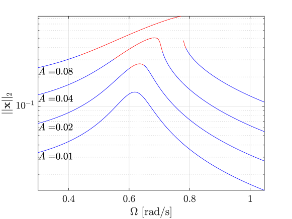
Figure 2: Example 1 with the nonlinearity (70) and the forcing (69), and the non-dimensional parameters $m=1$, $k=1$ and $c=0.3$: We use sequential continuation with the Picard iteration (blue) to capture the nonlinear frequency response curves for different amplitudes of loading. For relatively high amplitudes and near-resonant loading, the Picard approach fails to converge as expected. We then switch to the Newton–Raphson method (red). Indeed, using sequential continuation, the Newton–Raphson approach is unable to capture the fold developing in the forced response for high amplitudes (cf. Figure 3).

Performance comparison between the integral equations and the po toolbox of

coco

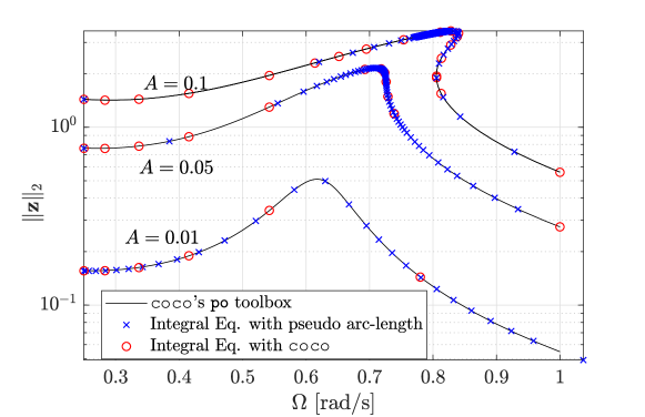
Figure 3: Steady-state responses obtained for Example 1 (with nonlinearity (70) and forcing (69)) from different continuation techniques. Numerical continuation using coco or pseudo-arc-length technique is able to capture the fold appearing in the response curve for $A=1$ (cf. Figure 3). Table 1 compares the computational performance of different methods on this example.

Forcing amplitude	Computation time [seconds (# continuation steps)]
	po-toolbox of coco	Integral eq. with in-house continuation	Integral eq. with coco continuation
0.01	16 (88 steps)	0.15 (28 steps)	2 (56 steps)
0.05	26 (124 steps)	3.89 (700 steps)	5 (110 steps)
0.1	32 (139 steps)	298.73 (38537 steps)	8 (160 steps)

Table 1: Comparison of computational performance for different continuation approaches

As shown in Table 1, the integral-equation approach proposed in the present paper is substantially faster than the po toolbox for continuation of periodic orbits with the MATLAB^®-based continuation package coco [11] for low enough amplitudes. However, as the frequency response starts developing complicated folds for higher amplitudes (cf. Figure 3), a much higher number of continuation steps are required for the convergence of our simple implementation of the pseudo-arc length continuation (cf. the third column in Table 1). Since coco is capable of performing continuation on general problems with advanced algorithms, we have implemented our integral-equation approach in coco in order to overcome this limitation. As shown in Table 1, the integral equation approach, along with coco’s built-in continuation scheme, is much more efficient for high-amplitude loading than any other method we have considered.

The integral-equation-based continuation was performed with $n_{t}=50$ time steps to discretize the solution in the time domain. On the other hand, the po toolbox in coco performs collocation-based continuation of periodic orbits, whereby it is able to modify the time-step discretization in an adaptive manner to optimize performance. In principle, it is possible to build an integral-equation-based toolbox in coco, which would allow for the adaptive selection of the discretization steps. This is expected to further increase the performance of integral equations approach, when equipped with coco for continuation.

5.1.2 Quasi-periodic forcing

Unlike the shooting technique reviewed earlier, our approach can also be applied to quasi-periodically forced systems (cf. Theorems 2 and 4). Therefore, we can also choose a quasi-periodic forcing of the form

$$f_{2}(t)=0,\quad f_{1}=0.01(\sin(\Omega_{1}t)+\sin(\Omega_{2}t))\,,\quad\kappa_{1}\Omega_{1}+\kappa_{2}\Omega_{2}\neq 0\,,\quad\kappa_{1},\kappa_{2}\in\mathbb{Z}-\{0\},$$ (71)

in Example 2, with the nonlinearity still given by eq. (70). Choosing the first forcing frequency $\Omega_{1}$ close to the first eigenfrequency $\omega_{1}$ and the second forcing frequency $\Omega_{2}$ close to $\omega_{2}$, we obtain the results depicted in Figure 4. We show the maximal displacement as a function of the two forcing frequencies, which are always selected to be incommensurate, otherwise the forcing would not be quasi-periodic. We nevertheless connect the resulting set of disrete points with a surface in Figure 4 for better visibility.

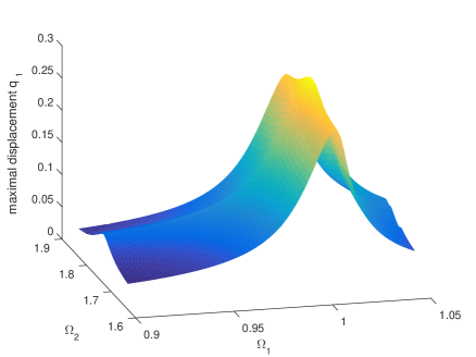
Figure 4: Response curve for Example 1 with the nonlinearity (70) and the forcing (71), and the non-dimensional parameters $m=1$, $k=1$ and $c=0.02$.

To carry out the quasi-periodic Picard iteration (56), the infinite summation involved in the formula has to be truncated. We chose to truncate the Fourier expansion once its relative error is within $10^{-3}$. If the iteration (56) did not converge, we switched to the Newton–Raphson scheme described in Section 3.2.2. In that case, we only kept the first three harmonics as Fourier basis.

Figure 5 shows the number of iterations needed to converge to a solution with this iteration procedure. Especially away from the resonances, a low number of iterations suffices for convergence to an accurate result. Also included in Figure 5 are the conditions (53) and (54), which guarantee the convergence for the iteration to the steady state solution of system (1). Outside the two red curves both (53) and (54) are satisfied and, accordingly, the iteration is guaranteed to converge. Since these conditions are only sufficient for convergence, the iteration converges also for frequency pairs within the red curves. The number of iterations required increases gradually and within the white region bounded by green lines, the Picard iteration fails. In such cases, we proceed to employ the Newton–Raphson scheme (cf. section (3.2.2)).

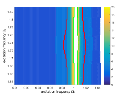
Figure 5: Number of iterations needed on the construction of Figure 4. Red curves bound the a priori guaranteed region of convergence for the Picard iteration. The white region is the domain where this iteration fails. In this region, we employ the Newton–Raphson scheme (cf. Section 3.2.2).

5.1.3 Non-smooth nonlinearity

As noted earlier, our iteration schemes are also applicable to non-smooth system as long as they are still Lipschitz. We select the nonlinearity of the form

$$S(q_{1})=\begin{cases}\alpha\text{sign}(q_{1})(|q_{1}|-\beta),&\textrm{for }|q_{1}|>\beta,\\ 0,&\textrm{otherwise},\end{cases}$$ (72)

which represents a hardening ($\alpha>0$) or softening ($\alpha<0$) spring with play $\beta>0$. The spring coefficient is given by $\tan^{-1}(\alpha)$, as depicted in Figure 6.

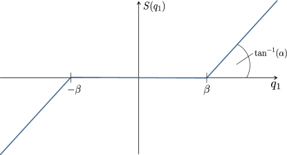
Figure 6: Graph of the non-smooth nonlinearity (72).

If we apply the forcing

$$f_{1}(t)=0.02\sin(\Omega t),\quad f_{2}(t)=0$$

to system (68) with the nonlinearity (72), our iteration techniques yield the response curve depicted in Figure 7. The Picard iteration approach (49) converges for moderate amplitudes, also in the nonlinear regime ($|q_{1}|>\beta$). When the Picard iteration fails at higher amplitudes, we employ the Newton–Raphson iteration. These results match closely with the amplitudes obtained by numerical integration, as seen in Figure 7.

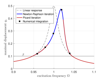
Figure 7: Response curve for Example 1 with the nonlinearity (72) and the forcing (69); parameters: $m=1$, $k=1$ and $c=0.02$, $\alpha=\beta=0.1$.

5.2 Nonlinear oscillator chain

Figure 8: An $n$-mass oscillator chain with coupled nonlinearity. We select the non-dimensional parameters $m=1$, $k=1,\kappa=0.5$ and $c=1$.

To illustrate the applicability of our results to higher-dimensional systems and more complex nonlinearities, we consider a modification of the oscillator chain studied by Breunung and Haller [9]. Shown Figure (8), the oscillator chain consists of $n$ masses with linear and cubic nonlinear springs coupling every pair of adjacent masses. Thus, the nonlinear function $\mathbf{S}$ is given as:

$$\mathbf{S}(\mathbf{x})=\kappa\left[\begin{array}[]{c}x_{1}^{3}-\left(x_{2}-x_{1}\right)^{3}\\ \left(x_{2}-x_{1}\right)^{3}-\left(x_{3}-x_{2}\right)^{3}\\ \left(x_{3}-x_{2}\right)^{3}-\left(x_{4}-x_{3}\right)^{3}\\ \vdots\\ \left(x_{n-1}-x_{n-2}\right)^{3}-\left(x_{n}-x_{n-1}\right)^{3}\\ \left(x_{2}-x_{1}\right)^{3}+x_{n}^{3}\end{array}\right].$$

The frequency response curve obtained with the iteration described in section 3.2 for harmonic forcing is shown in Figure 9 for $20$ degrees-of-freedom. We also include the frequency response obtained with the po-toolbox of coco [11] with default settings for comparison. The integral equations approach gives the same solution as the po-toolbox of coco, but the difference in run times is stunning: the po-toolbox of coco takes about 12 minutes and 59 seconds to generate this frequency response curve, whereas the integral-equation approach with a naive sequential continuation strategy takes 13 seconds to generate the same curve. This underlines the power of the approches proposed here for complex mechanical vibrations.

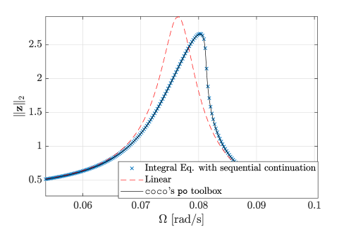
Figure 9: Comparison of frequency sweeps produced using different continuation techniques for a 20-DOF oscillator chain with coupled nonlinearity.

6 Conclusion

We have presented an integral-equation approach for the fast computation of the steady-state response of nonlinear dynamical systems under external (quasi-) periodic forcing. Starting with a forced linear system, we derive integral equations that must be satisfied by the steady-state solutions of the full nonlinear system. The kernel of the integral equation is a Green’s function, which we calculate explicitly for general mechanical systems. Due to these explicit formulae, the convolution with the Green’s function can be performed with minimal effort, thereby making the solution of the equivalent integral equation significantly faster than full time integration of the dynamical system. We also show the applicability of the same equations to compute periodic orbits of unforced, conservative systems.

We employ a combination of Picard and the Newton–Raphson iterations to solve the integral equations for the steady-state response. Since the Picard iteration requires only a simple application of a nonlinear map (and no direct solution via operator inversion), it is especially appealing for high-dimensional system. Furthermore, the nonlinearity only needs to be Lipschitz continuous, therefore our approach also applies to non-smooth systems, as we demonstrated numerically in section 5.1.3. We establish a rigorous a priori estimate for the convergence of the Picard iteration. From this estimate, we conclude that the convergence of the Picard iteration becomes problematic for high amplitudes and forcing frequencies near resonance with an eigenfrequency of the linearized system. This can also be observed numerically in Example 5.1.1, where the Picard iteration fails close to resonance.

To capture the steady-state response for a full frequency sweep (including high amplitudes and resonant frequencies), we deploy the Newton–Raphson iteration once the Picard iteration fails near resonance. The Newton–Raphson formulation can be computationally-intensive as it requires a high-dimensional operator inversion, which would normally make this type of iteration potenially unfeasible for exceedingly high-dimensional systems. However, we circumvent this problem with the Newton–Raphson method using modifications discussed in Section 3.2.

We have further demonstrated that advanced numerical continuation is required to compute the (quasi-) periodic response when folds appear in solution branches. To this end, we formulated one such continuation scheme, i.e., the pseudo arc-length scheme, in our integral equations setting to facilitate capturing response around such folds. We also demonstrated that the integral equations approach can be coupled with existing state-of-the-art continuation packages to obtain better performance (cf. Section 5.1.1).

Compared to well-established shooting-based techniques, our integral-equation approach also calculates quasi-periodic responses of dynamical systems and avoids numerical time integration. The latter can be computationally expensive for high-dimensional or stiff systems. In the case of purely geometric (position-dependent) nonlinearities, we can reduce the dimensionality of the corresponding integral iteration by half, by iterating on the position vector only. For numerical examples, we show that our integral equation approach equipped with numerical continuation outperforms available continuation packages significantly. As opposed to the broadly used harmonic balance procedure (cf. Chua and Ushida [10] and Lau and Cheung [20]), our approach also gives a computable and rigorous existence criterion for the (quasi-) periodic response of the system.

Along with this work, we provide a MATLAB^® code with a user-friendly implementation of the developed iterative schemes. This code implements the cheap and fast Picard iteration, as well as the robust Newton–Raphson iteration, along with sequential/pseudo-arc length continuation. We have further tested our approach in combination with the MATLAB^®-based continuation package coco [11] and obtained an improvement in performance. One could, therefore, further add an integral-equation-based toolbox to coco with adaptive time steps in the discretization to obtain better efficiency.

Acknowledgments

We are thankful to Harry Dankowicz and Mingwu Li for clarifications and help with the continuation package coco [11]. We also acknowledge helpful discussions with Mark Mignolet and Dane Quinn.

Appendix A Proof of Lemma 1

The general solution of (6) is given by the classic variation of constants formula

$$\mathbf{w}(t)=e^{\boldsymbol{\Lambda}t}\mathbf{w}(0)+\int_{0}^{t}e^{\boldsymbol{\Lambda}(t-s)}\boldsymbol{\psi}(s)\,ds.$$ (73)

If $\mathbf{w}_{0}(t)$ is the unique $T$-periodic solution of (6), then we obtain from (73) that

$$\mathbf{w}_{0}(T)=e^{\boldsymbol{\Lambda}T}\mathbf{w}_{0}(0)+\int_{0}^{T}e^{\boldsymbol{\Lambda}(T-s)}\boldsymbol{\psi}(s)\,ds=\mathbf{w}_{0}(0).$$

This gives the initial condition for the periodic solution as

$$\mathbf{w}_{0}(0)=\left[\mathbf{I}-e^{\boldsymbol{\Lambda}T}\right]^{-1}\int_{0}^{T}e^{\boldsymbol{\Lambda}(T-s)}\boldsymbol{\psi}(s)\,ds.$$ (74)

Note that the matrix $\left[\mathbf{I}-e^{\boldsymbol{\Lambda}T}\right]$ is invertible due to the non-resonance condition (7). Substitution of the initial condition from (74) into the general solution (73), we obtain an expression for the unique $T$-periodic solution $\mathbf{w}_{0}(t)$ to (6) as

$$\mathbf{w}_{0}(t) =e^{\boldsymbol{\Lambda}t}\left[\mathbf{I}-e^{\boldsymbol{\Lambda}T}\right]^{-1}\int_{0}^{T}e^{\boldsymbol{\Lambda}(T-s)}\boldsymbol{\psi}(s)\,ds+\int_{0}^{t}e^{\boldsymbol{\Lambda}(t-s)}\boldsymbol{\psi}(s)\,ds$$

$$=e^{\boldsymbol{\Lambda}T}\left[\mathbf{I}-e^{\boldsymbol{\Lambda}T}\right]^{-1}\int_{0}^{T}e^{\boldsymbol{\Lambda}(t-s)}\boldsymbol{\psi}(s)\,ds+\int_{0}^{t}e^{\boldsymbol{\Lambda}(t-s)}\boldsymbol{\psi}(s)\,ds$$ (75)

$$=e^{\boldsymbol{\Lambda}T}\left[\mathbf{I}-e^{\boldsymbol{\Lambda}T}\right]^{-1}\int_{0}^{t}e^{\boldsymbol{\Lambda}(t-s)}\boldsymbol{\psi}(s)\,ds+e^{\boldsymbol{\Lambda}T}\left[\mathbf{I}-e^{\boldsymbol{\Lambda}T}\right]^{-1}\int_{t}^{T}e^{\boldsymbol{\Lambda}(t-s)}\boldsymbol{\psi}(s)\,ds+\int_{0}^{t}e^{\boldsymbol{\Lambda}(t-s)}\boldsymbol{\psi}(s)\,ds$$

$$=\int_{0}^{t}\left[e^{\boldsymbol{\Lambda}T}\left[\mathbf{I}-e^{\boldsymbol{\Lambda}T}\right]^{-1}+\mathbf{I}\right]e^{\boldsymbol{\Lambda}(t-s)}\boldsymbol{\psi}(s)\,ds+\int_{t}^{T}e^{\boldsymbol{\Lambda}T}\left[\mathbf{I}-e^{\boldsymbol{\Lambda}T}\right]^{-1}e^{\boldsymbol{\Lambda}(t-s)}\boldsymbol{\psi}(s)\,ds$$

$$=\int_{0}^{T}\underbrace{\left[e^{\boldsymbol{\Lambda}T}\left[\mathbf{I}-e^{\boldsymbol{\Lambda}T}\right]^{-1}+h(t-s)\mathbf{I}\right]e^{\boldsymbol{\Lambda}(t-s)}}_{\mathbf{G}(t-s,T)}\boldsymbol{\psi}(s)\,ds\,,$$

where $\mathbf{G}(t,T)$ is a diagonal matrix with the entries given by (9). Using the linear modal transformation $\mathbf{z}_{P}=\mathbf{Vw}_{0}$, we find the unique $T$-periodic solution to (4) in the form

$$\mathbf{z}_{P}(t)=\mathbf{V}\int_{0}^{T}\mathbf{G}(t-s,T)\boldsymbol{\psi}(s)\,ds.$$

Appendix B Proof of Theorem 1

If $\mathbf{z}(t)$ is a $T$-periodic solution of (3), then it satisfies the linear inhomogeneous differential equation

$$\mathbf{B}\dot{\mathbf{z}}=\mathbf{A}\mathbf{z}+\mathbf{F}(t)-\mathbf{R}(\mathbf{z}(t)),$$

where we view $\mathbf{F}(t)-\mathbf{R}(\mathbf{z}(t))$ as a $T-$periodic forcing term. Thus, according to Lemma 1, we have

$$\mathbf{z}(t)=\mathbf{V}\int_{0}^{T}\mathbf{G}(t-s,T)\mathbf{V}^{-1}\left[\mathbf{F}(s)-\mathbf{R}(\mathbf{z}(s))\right]\,ds,$$

as claimed in statement (i).

Now, let $\mathbf{z}(t)$ be a continuous, $T-$periodic solution to (11). After introducing the notation $\boldsymbol{\chi}(t)=\mathbf{V}^{-1}\left[\mathbf{F}(t)-\mathbf{R}(\mathbf{z}(t))\right]$, we have

$$\mathbf{z}(t) =\mathbf{V}\int_{0}^{T}\mathbf{G}(t-s,T)\boldsymbol{\chi}(s)\,ds,$$

$$=\mathbf{V}e^{\boldsymbol{\Lambda}t}\left(\mathbf{I}-e^{\boldsymbol{\Lambda}T}\right)^{-1}\int_{0}^{T}e^{\boldsymbol{\Lambda}(T-s)}\boldsymbol{\chi}(s)\,ds+\mathbf{V}\int_{0}^{t}e^{\boldsymbol{\Lambda}(t-s)}\boldsymbol{\chi}(s)\,ds\,,$$ (76)

where (76) is a direct consequence of (75). By the continuity of $\mathbf{z}(t)$, $\boldsymbol{\chi}(t)$ is also at least $C^{0}$ ($\mathbf{F}$ is at least $C^{0}$ and $\mathbf{R}$ is Lipschitz). Thus, for any $t\in[0,T]$, the right-hand side of (76) can be differentiated with respect to $t$ according to the Leibniz rule, to obtain

$$\frac{d\mathbf{z}(t)}{dt} =\mathbf{V}\boldsymbol{\Lambda}e^{\boldsymbol{\Lambda}t}\left(\mathbf{I}-e^{\boldsymbol{\Lambda}T}\right)^{-1}\int_{0}^{T}e^{\boldsymbol{\Lambda}(T-s)}\boldsymbol{\chi}(s)\,ds+\mathbf{V}\boldsymbol{\Lambda}\int_{0}^{t}e^{\boldsymbol{\Lambda}(t-s)}\boldsymbol{\chi}(s)\,ds\,+\mathbf{V}\boldsymbol{\Lambda}\boldsymbol{\chi}(t)$$

$$=\mathbf{V}\boldsymbol{\Lambda}\mathbf{V}^{-1}\mathbf{z}(t)+\mathbf{V}\boldsymbol{\Lambda}\boldsymbol{\chi}(t)\qquad\text{(using \eqref{eq:temp1})}$$

$$=\mathbf{V}\boldsymbol{\Lambda}\mathbf{V}^{-1}\mathbf{z}(t)+\mathbf{V}\boldsymbol{\Lambda}\mathbf{V}^{-1}\left[\mathbf{F}(t)-\mathbf{R}(\mathbf{z}(t))\right],$$

which implies

$$\mathbf{B}\frac{d\mathbf{z}(t)}{dt}=\mathbf{A}\mathbf{z}(t)+\mathbf{F}(t)-\mathbf{R}(\mathbf{z}(t)),$$

as claimed in statement (ii).

Appendix C Proof of Lemma 2

By the linearity of (4), one can verify that the sum of periodic solutions given by Lemma 1 for each periodic forcing summand in (12) is the unique, bounded solution of (4). In case of a forcing written as a Fourier series, we can carry out the integration appearing in Lemma 1 for each summand in this bounded solution explicitly in diagonalized coordinates $\mathbf{z}=\mathbf{V}\mathbf{w}$. With the notation $\boldsymbol{\psi_{\boldsymbol{\kappa}}}=\mathbf{V}^{-1}\mathbf{F}_{\boldsymbol{\kappa}}$, we then obtain for the $j^{\text{th}}$ degree of freedom:

$$w_{j}(t) =\sum_{\boldsymbol{\kappa}\in\mathbb{Z}^{k}}\int_{0}^{T_{\boldsymbol{\kappa}}}G_{j}(t-s,T_{\boldsymbol{\kappa}})\psi_{\boldsymbol{\kappa},j}e^{i\left\langle\boldsymbol{\kappa},\boldsymbol{\Omega}\right\rangle s}\,ds$$

$$=\sum_{\boldsymbol{\kappa}\in\mathbb{Z}^{k}}\int_{0}^{T_{\boldsymbol{\kappa}}}e^{\lambda_{j}t}\left(\frac{e^{\lambda_{j}T_{\boldsymbol{\kappa}}}}{1-e^{\lambda_{j}T_{\boldsymbol{\kappa}}}}+h(t)\right)\psi_{\boldsymbol{\kappa},j}e^{i\left\langle\boldsymbol{\kappa},\boldsymbol{\Omega}\right\rangle s}\,ds$$

$$=\sum_{\boldsymbol{\kappa}\in\mathbb{Z}^{k}}\int_{0}^{t}e^{\lambda_{j}(t-s)}\left(\frac{1}{1-e^{\lambda_{j}T_{\boldsymbol{\kappa}}}}\right)\psi_{\boldsymbol{\kappa},j}e^{i\left\langle\boldsymbol{\kappa},\boldsymbol{\Omega}\right\rangle s}\,ds+\sum_{\boldsymbol{\kappa}\in\mathbb{Z}^{k}}\int_{t-s}^{T_{\boldsymbol{\kappa}}}e^{\lambda_{j}(t-s)}\left(\frac{e^{\lambda_{j}T_{\boldsymbol{\kappa}}}}{1-e^{\lambda_{j}T_{\boldsymbol{\kappa}}}}\right)\psi_{\boldsymbol{\kappa},j}e^{i\left\langle\boldsymbol{\kappa},\boldsymbol{\Omega}\right\rangle s}\,ds$$

$$=\sum_{\boldsymbol{\kappa}\in\mathbb{Z}^{k}}e^{\lambda_{j}t}\left(\frac{1}{1-e^{\lambda_{j}T_{\boldsymbol{\kappa}}}}\right)\psi_{\boldsymbol{\kappa},j}\int_{0}^{t}e^{-\lambda_{j}s}e^{i\left\langle\boldsymbol{\kappa},\boldsymbol{\Omega}\right\rangle s}\,ds+\sum_{\boldsymbol{\kappa}\in\mathbb{Z}^{k}}e^{\lambda_{j}t}\left(\frac{e^{\lambda_{j}T_{\boldsymbol{\kappa}}}}{1-e^{\lambda_{j}T_{\boldsymbol{\kappa}}}}\right)\psi_{\boldsymbol{\kappa},j}\int_{t}^{T_{\boldsymbol{\kappa}}}e^{-\lambda_{j}s}e^{i\left\langle\boldsymbol{\kappa},\boldsymbol{\Omega}\right\rangle s}\,ds$$

$$=\sum_{\boldsymbol{\kappa}\in\mathbb{Z}^{k}}e^{\lambda_{j}t}\left(\frac{1}{1-e^{\lambda_{j}T_{\boldsymbol{\kappa}}}}\right)\psi_{\boldsymbol{\kappa},j}\frac{1}{i\left\langle\boldsymbol{\kappa},\boldsymbol{\Omega}\right\rangle-\lambda_{j}}\left.e^{(i\left\langle\boldsymbol{\kappa},\boldsymbol{\Omega}\right\rangle-\lambda_{j})s}\right|_{s=0}^{s=t}+$$

$$\quad\sum_{\boldsymbol{\kappa}\in\mathbb{Z}^{k}}e^{\lambda_{j}t}\left(\frac{e^{\lambda_{j}T_{\boldsymbol{\kappa}}}}{1-e^{\lambda_{j}T_{\boldsymbol{\kappa}}}}\right)\psi_{\boldsymbol{\kappa},j}\frac{1}{i\left\langle\boldsymbol{\kappa},\boldsymbol{\Omega}\right\rangle-\lambda_{j}}\left.e^{(i\left\langle\boldsymbol{\kappa},\boldsymbol{\Omega}\right\rangle-\lambda_{j})s}\right|_{s=t}^{s=T_{\boldsymbol{\kappa}}}$$

$$=\sum_{\boldsymbol{\kappa}\in\mathbb{Z}^{k}}e^{\lambda_{j}t}\left(\frac{1}{1-e^{\lambda_{j}T_{\boldsymbol{\kappa}}}}\right)\psi_{\boldsymbol{\kappa},j}\frac{1}{i\left\langle\boldsymbol{\kappa},\boldsymbol{\Omega}\right\rangle-\lambda_{j}}\left[e^{(i\left\langle\boldsymbol{\kappa},\boldsymbol{\Omega}\right\rangle-\lambda_{j})t}-1+e^{\lambda_{j}T_{\boldsymbol{\kappa}}}(e^{(i\left\langle\boldsymbol{\kappa},\boldsymbol{\Omega}\right\rangle-\lambda_{j})T_{\boldsymbol{\kappa}}}-e^{(i\left\langle\boldsymbol{\kappa},\boldsymbol{\Omega}\right\rangle-\lambda_{j})t})\right]$$

$$=\sum_{\boldsymbol{\kappa}\in\mathbb{Z}^{k}}e^{\lambda_{j}t}\psi_{\boldsymbol{\kappa},j}\frac{1}{i\left\langle\boldsymbol{\kappa},\boldsymbol{\Omega}\right\rangle-\lambda_{j}}\frac{1}{1-e^{\lambda_{j}T_{\boldsymbol{\kappa}}}}\left[(1-e^{\lambda_{j}T_{\boldsymbol{\kappa}}})(e^{(i\left\langle\boldsymbol{\kappa},\boldsymbol{\Omega}\right\rangle-\lambda_{j})t})-1+e^{i\left\langle\boldsymbol{\kappa},\boldsymbol{\Omega}\right\rangle T_{\boldsymbol{\kappa}}}\right]$$

$$=\sum_{\boldsymbol{\kappa}\in\mathbb{Z}^{k}}\frac{1}{i\left\langle\boldsymbol{\kappa},\boldsymbol{\Omega}\right\rangle-\lambda_{j}}\psi_{\boldsymbol{\kappa},j}e^{i\left\langle\boldsymbol{\kappa},\boldsymbol{\Omega}\right\rangle t}\,.$$

Appendix D Explicit Green’s function for mechanical systems: Proof of Lemma 3

The first-order ODE formulation for (26) is given by

$$\frac{d}{dt}\left(\begin{array}[]{c}y_{j}\\ \dot{y}_{j}\end{array}\right)=\underbrace{\left(\begin{array}[]{cc}0&1\\ -\omega_{0,j}^{2}&-2\zeta_{j}\omega_{0,j}\end{array}\right)}_{\mathbf{A}_{j}}\left(\begin{array}[]{c}y_{j}\\ \dot{y}_{j}\end{array}\right)+\left(\begin{array}[]{c}0\\ \varphi_{j}(t)\end{array}\right),\qquad j=1,\ldots,n.$$ (77)

By the classic variation of constants formula for first-order systems of ordinary differential equations, the general solution of (77) is of the form

$$\left(\begin{array}[]{c}y_{j}(t)\\ \dot{y}_{j}(t)\end{array}\right)=\mathbf{N}^{(j)}(t)\left(\begin{array}[]{c}y_{j}(0)\\ \dot{y}_{j}(0)\end{array}\right)+\int_{0}^{t}\mathbf{N}^{(j)}(t-s)\left(\begin{array}[]{c}0\\ \varphi_{j}(s)\end{array}\right)ds,\qquad j=1,\ldots,n,$$ (78)

with $\mathbf{N}(t)=e^{\mathbf{A}_{j}t}$ denoting the fundamental matrix solution for the $j^{th}$ mode with $\mathbf{N}(0)=\mathbf{I}.$ Thus, the homogeneous (unforced) version of (26), the explicit solution can be obtained as

$$\left(\begin{array}[]{c}y_{j}(t)\\ \dot{y}_{j}(t)\end{array}\right)=\mathbf{N}^{(j)}(T)\left(\begin{array}[]{c}y_{j}(0)\\ \dot{y}_{j}(0)\end{array}\right),\qquad j=1,\ldots,n.$$ (79)

Since $\mathbf{F}(t)$ is uniformly bounded for all times and all $\mathbf{A}_{j}$ matrices are hyperbolic ($\zeta_{j}>0$ for $j=1,...,n$), then a unique uniformly bounded solution exists for the $2n$-dimensional system of linear ordinary differential equations (ODEs) (77) (see, e.g., Burd [8]). The initial condition $\left(y_{j}(0),\dot{y}_{j}(0)\right)$ for the unique $T$-periodic solution of (78) is obtained by imposing periodicity, i.e., $y_{j}(0)=y_{j}(T)$ for $j=1,\dots,n$ and is given by

$$\left(\begin{array}[]{c}y_{j}(0)\\ y_{j}(0)\end{array}\right) =\frac{1}{1-\text{Trace}\left(\mathbf{N}^{(j)}(T)\right)+\text{det}\left(\mathbf{N}^{(j)}(T)\right)}\int_{0}^{T}\left(\begin{array}[]{c}\left(1-N_{22}^{(j)}(T)\right)N_{12}^{(j)}(T-s)+N_{12}^{(j)}(T)N_{22}^{(j)}(T-s)\\ \left(1-N_{11}^{(j)}(T)\right)N_{22}^{(j)}(T-s)+N_{21}^{(j)}(T)N_{12}^{(j)}(T-s)\end{array}\right)\varphi_{j}(s)\,ds\,.$$ (84)

Finally, the unique periodic response $\left(y_{j}(t),\dot{y}_{j}(t)\right)$ is obtained by substituting the initial condition (84) into the Duhamel’s integral formula (78) as

$$\left(\begin{array}[]{c}y_{j}(t)\\ \dot{y}_{j}(t)\end{array}\right) =\frac{\mathbf{N}^{(j)}(t)}{1-\text{Trace}\left(\mathbf{N}^{(j)}(T)\right)+\text{det}\left(\mathbf{N}^{(j)}(T)\right)}\int_{0}^{T}\left(\begin{array}[]{c}\left(1-N_{22}^{(j)}(T)\right)N_{12}^{(j)}(T-s)+N_{12}^{(j)}(T)N_{22}^{(j)}(T-s)\\ \left(1-N_{11}^{(j)}(T)\right)N_{22}^{(j)}(T-s)+N_{21}^{(j)}(T)N_{12}^{(j)}(T-s)\end{array}\right)\varphi_{j}(s)\,ds$$ (89)

$$\quad+\int_{0}^{t}\mathbf{N}^{(j)}(t-s)\left(\begin{array}[]{c}0\\ \varphi_{j}(s)\end{array}\right)ds,\qquad j=1,\ldots,n\,.$$ (92)

With the notation introduced in (27), i.e.,

$$\alpha_{j}:=\text{Re}(\lambda_{2j}),\quad\omega_{j}:=|\text{Im}(\lambda_{2j})|,\quad\beta_{j}:=\alpha_{j}+\omega_{j},\quad\gamma_{j}:=\alpha_{j}-\omega_{j,}\quad j=1,\dots,n,$$

the specific expressions for the fundamental matrix of solutions of (77) in the under-damped, the critically-damped and the over-damped case are given by

$$\mathbf{N}^{(j)}(t)=\begin{cases}\frac{e^{\alpha_{j}t}}{\omega_{j}}\left(\begin{array}[]{cc}\omega_{j}\cos\omega_{j}t-\alpha_{j}\sin\omega_{j}t&\sin\omega_{j}t\\ -\alpha_{j}^{2}\sin\omega_{j}t-\omega_{j}^{2}\sin\omega_{j}t&\omega_{j}\cos\omega_{j}t+\alpha_{j}\sin\omega_{j}t\end{array}\right),&\zeta_{j}<1\\ \left(\begin{array}[]{cc}e^{\alpha_{j}t}-\alpha_{j}te^{\alpha_{j}t}&te^{\alpha_{j}t}\\ -\alpha_{j}^{2}te^{\alpha_{j}t}&e^{\alpha_{j}t}+\alpha_{j}te^{\alpha_{j}t}\end{array}\right)\,,&\zeta_{j}=1\\ \frac{1}{\beta_{j}-\gamma_{j}}\left(\begin{array}[]{cc}\beta_{j}e^{\gamma_{j}t}-\alpha_{j}e^{\beta_{j}t}&e^{\beta_{j}t}-e^{\gamma_{j}t}\\ \gamma_{j}\beta_{j}\left(e^{\gamma_{j}t}-e^{\beta_{j}t}\right)&\beta_{j}e^{\beta_{j}t}-\gamma_{j}e^{\gamma_{j}t}\end{array}\right)\,,&\zeta_{j}>1\end{cases},\quad j=1,\dots,n\,.$$ (93)

Furthermore, we have

$$\mathrm{Trace\,}\mathbf{N}^{(j)}(t) =\begin{cases}2e^{\alpha_{j}t}\cos\omega_{j}t\,,&\zeta_{j}<1\\ 2e^{\beta_{j}t}\,,&\zeta_{j}=1\\ e^{\beta_{j}t}+e^{\gamma_{j}t}\,,&\zeta_{j}>1\end{cases},\quad j=1,\dots,n\,.$$

$$\det\mathbf{N}^{(j)}(t) =\begin{cases}e^{2\alpha_{j}t}\,,&\zeta_{j}<1\\ e^{2\beta_{j}t}\,,&\zeta_{j}=1\\ e^{\left(\beta_{j}+\gamma_{j}\right)t}\,,&\zeta_{j}>1\end{cases},\quad j=1,\dots,n\,.$$ (94)

Thus, we can explicitly compute the particular periodic solution given in (92) using (93) as

$$\mathbf{y}(t)=\int_{0}^{T}\mathbf{L}(t-s,T)\boldsymbol{\varphi}(s)\,ds,\quad\mathbf{L}(t-s,T)=\mathrm{diag}\left(L_{1}(t-s,T),\ldots,L_{n}(t-s,T)\right)\in\mathbb{R}^{n\times n},$$

$$\dot{\mathbf{y}}(t)=\int_{0}^{T}\mathbf{J}(t-s,T)\boldsymbol{\varphi}(s)\,ds,\quad\mathbf{J}(t-s,T)=\mathrm{diag}\left(J_{1}(t-s,T),\ldots,J_{n}(t-s,T)\right)\in\mathbb{R}^{n\times n},$$

with the diagonal elements of the Green’s function matrices $\mathbf{L,J}$ defined in (29) and (31),i.e.,

$$L_{j}(t,T)=\begin{cases}\frac{e^{\alpha_{j}t}}{\omega_{j}}\left[\frac{e^{\alpha_{j}T}\left[\sin\omega_{j}(T+t)-e^{\alpha_{j}T}\sin\omega_{j}t\right]}{1+e^{2\alpha_{j}T}-2e^{\alpha_{j}T}\cos\omega_{j}T}+h(t)\sin\omega_{j}t\right],&\zeta_{j}<1\\ \frac{e^{\alpha_{j}(T+t)}\left[\left(1-e^{\alpha_{j}T}\right)t+T\right]}{\left(1-e^{\alpha_{j}T}\right)^{2}}+h(t)te^{\alpha_{j}t}\,,&\zeta_{j}=1\\ \frac{1}{(\beta_{j}-\gamma_{j})}\left[\frac{e^{\beta_{j}(T+t)}\left(1-e^{\gamma_{j}T}\right)-e^{\gamma_{j}(T+t)}\left(1-e^{\beta_{j}T}\right)}{1-e^{\gamma_{j}T}-e^{\beta_{j}T}+e^{\left(\gamma_{j}+\beta_{j}\right)T}}+h(t)\left(e^{\beta_{j}t}-e^{\gamma_{j}t}\right)\right],&\zeta_{j}>1\end{cases},$$

$$\begin{split}J_{j}(t,T)&=\begin{cases}\begin{array}[]{c}\frac{e^{\alpha_{j}t}}{\omega_{j}}\left[\frac{e^{\alpha_{j}T}\left[\omega_{j}\left(\cos\omega_{j}(T+t)-e^{\alpha_{j}T}\cos\omega_{j}t\right)+\alpha_{j}\left(\sin\omega_{j}(T+t)-e^{\alpha_{j}T}\sin\omega_{j}t\right)\right]}{1+e^{2\alpha_{j}T}-2e^{\alpha_{j}T}\cos\omega_{j}T}+\right.\\ \left.h(t)\left(\frac{1}{\omega_{j}}\cos\omega_{j}t+\alpha_{j}\sin\omega_{j}t\right)\right]\end{array}\quad,&\zeta_{j}<1\\ \frac{e^{\alpha_{j}(T+t)}\left[\left(1-e^{\alpha_{j}T}\right)\left(1+\alpha_{j}t\right)+\alpha_{j}T\right]}{\left(1-e^{\alpha_{j}T}\right)^{2}}+h(t)\left(e^{\alpha_{j}t}+\alpha_{j}te^{\alpha_{j}t}\right)\,,&\zeta_{j}=1\\ \frac{1}{(\beta_{j}-\gamma_{j})}\left[\frac{\beta_{j}e^{\beta_{j}(T+t)}\left(1-e^{\gamma_{j}T}\right)-\gamma_{j}e_{j}^{\gamma_{j}(T+t)}\left(1-e^{\beta_{j}T}\right)}{1-e^{\gamma_{j}T}-e^{\beta_{j}T}+e^{\left(\gamma_{j}+\beta_{j}\right)T}}+h(t)\left(\beta_{j}e^{\beta_{j}t}-\gamma_{j}e^{\gamma_{j}t}\right)\right],&\zeta_{j}>1\end{cases}\end{split}\,,\quad j=1,\dots,n\,\,.$$

Finally, the linear periodic response $\mathbf{x}_{P}(t)$ in the original system coordinates can then obtained by the linear transformation $\mathbf{x}_{P}(t)=\mathbf{Uy}(t)$ as

$$\mathbf{x}_{P}(t)=\mathbf{U}\int_{0}^{T}\mathbf{L}(t-s,T)\mathbf{U}^{\top}\mathbf{f}(s)\,ds.$$

Appendix E Derivative of Green’s function with respect to $T$

The derivative with respect to the time period $T$ of the first-order periodic Green’s function $\mathbf{G}$ given in (9) is simply given by

$$\frac{\partial G_{j}}{\partial T}(t,T)=\lambda_{j}e^{\lambda_{j}t}\frac{e^{\lambda_{j}T}}{(1-e^{\lambda_{j}T})^{2}},\quad j=1,\dots,2n\,.$$ (95)

We also provide the derivative of the Green’s function $\mathbf{L}$ with respect to $T$ to ease the computation of the Jacobian of the zero function in during numerical continuation. This is obtained by simply differentiating (29) with respect to T. We use a symbolic toolbox for this procedure:

$$\frac{dL_{j}}{dT}(t,T)=\begin{cases}\begin{array}[]{c}\frac{e^{\alpha_{j}(t+T)}}{\omega_{j}\left(1+e^{2\alpha_{j}T}-2e^{\alpha_{j}T}\cos\omega_{j}T\right)^{2}}\left[\omega_{j}\cos\omega_{j}(T+t)+\alpha_{j}\sin\omega_{j}(T+t)\right.-\\ \left.2e^{\alpha_{j}T}\left(\omega_{j}\cos\omega_{j}t+\alpha_{j}\sin\omega_{j}t\right)+e^{2\alpha_{j}T}\left(\alpha_{j}\sin\omega_{j}(t-T)+\omega_{j}\cos\omega_{j}(t-T)\right)\right]\end{array},&\zeta_{j}<1\\ \frac{\alpha_{j}e^{\alpha_{j}(t+T)}}{(e^{\alpha_{j}T}-1)^{2}}\left[t+T-2te^{\alpha_{j}T}+1-\frac{2e^{\alpha_{j}T}(T-t(e^{\alpha_{j}T}-1))}{(e^{\alpha_{j}T}-1)}\right]&\zeta_{j}=1\\ \begin{array}[]{c}\frac{1}{(\beta_{j}-\gamma_{j})}\left[\frac{\left(\beta_{j}-\left(\gamma_{j}+\beta_{j}\right)e^{\gamma_{j}T}\right)e^{\beta_{j}(T+t)}+\left(\left(\gamma_{j}+\beta_{j}\right)e^{\beta_{j}T}-\gamma_{j}\right)e^{\gamma_{j}(T+t)}}{1-e^{\gamma_{j}T}-e^{\beta_{j}T}+e^{\left(\gamma_{j}+\beta_{j}\right)T}}+\right.\\ \left.\frac{\left(e^{\beta_{j}(T+t)}\left(1-e^{\gamma_{j}T}\right)-e^{\gamma_{j}(T+t)}\left(1-e^{\beta_{j}T}\right)\right)\left(\gamma_{j}e^{\gamma_{j}T}+\beta_{j}e^{\beta_{j}T}-\left(\gamma_{j}+\beta_{j}\right)e^{\left(\gamma_{j}+\beta_{j}\right)T}\right)}{\left(1-e^{\gamma_{j}T}-e^{\beta_{j}T}+e^{\left(\gamma_{j}+\beta_{j}\right)T}\right)^{2}}\right]\end{array}\,,&\zeta_{j}>1\end{cases},\quad j=1,\dots,n\,.$$

Appendix F Proof of Remark 2

We derive an estimate for the sup norm of the integral of the operator norm of the Green’s function, i.e., for $\int_{0}^{T}\left\|G_{j}(t-s,T)\right\|\,ds$ defined in equation (9). For $t>s$, we start by noting that

$$\left|G_{j}(t-s,T)\right|=\left|e^{\lambda_{j}(t-s)}\left(\frac{1}{1-e^{\lambda_{j}T}}\right)\right|\leq\left|e^{\lambda_{j}(t-s)}\right|\frac{1}{\left|1-e^{\lambda_{j}T}\right|}\leq\frac{\max(\left|e^{\lambda_{j}t}\right|,1)}{\left|1-e^{\lambda_{j}T}\right|},\quad 0\leq s\leq t<T.$$

For the case $T>s>t$, we obtain

$$\left|G_{j}(t-s,T)\right|=\left|e^{\lambda_{j}(t-s)}\left(\frac{e^{\lambda_{j}T}}{1-e^{\lambda_{j}T}}\right)\right| \leq\max\left(\left|\left(\frac{e^{\lambda_{j}T}}{1-e^{\lambda_{j}T}}\right)\right|,\left|e^{\lambda_{j}(t-T)}\left(\frac{e^{\lambda_{j}T}}{1-e^{\lambda_{j}T}}\right)\right|\right)$$

$$\leq\frac{\max(\left|e^{\lambda_{j}t}\right|,1)}{\left|1-e^{\lambda_{j}T}\right|},\quad 0\leq s\leq t<T.$$

The upper bounds on the Green’s function in the two intervals are equal and we therefore obtain

$$\left\|\int_{0}^{T}\left\|\mathbf{G}(t-s,T)\right\|\,ds\right\|_{0} =\max_{t\in[0,T]}\int_{0}^{T}\left\|\mathbf{G}(t-s,T)\right\|\,ds$$

$$\leq\max_{t\in[0,T]}\int_{0}^{T}\max_{1\leq j\leq n}\frac{\max(\left|e^{\lambda_{j}t}\right|,1)}{\left|1-e^{\lambda_{j}T}\right|}\,ds$$

$$\leq\max_{1\leq j\leq n}\frac{T\max(\left|e^{\lambda_{j}T}\right|,1)}{\left|1-e^{\lambda_{j}T}\right|}\eqqcolon\Gamma(T).$$

Appendix G Proof of Theorem 5

In the following, we derive conditions under which the mapping $\mathcal{\boldsymbol{\mathcal{H}}}$ defined in equation (36) is a contraction mapping. We rewrite (36) as

$$\mathbf{z}(t)=\Upsilon_{P}(\mathbf{F}(t)-\mathbf{R}(\mathbf{z}(t))):=\int_{0}^{T}\mathbf{V}\mathbf{G}(t-s,T)\mathbf{V}^{-1}\left[\mathbf{F}(s)-\mathbf{R}(\mathbf{z}(s))\right]\,ds,$$

where $\Upsilon_{P}$ is a linear map representing the convolution operation with the Green’s function. Specifically, we define the space of $n$-dimensional periodic $T$-periodic functions as

$$\mathcal{P}_{n}:=\{\mathbf{p}:\mathbb{R}\to\mathbb{R}^{n},\mathbf{p}\in C^{0},\mathbf{p}(t)=\mathbf{p}(t+T)\forall t\in\mathbb{R}\}.$$ (96)

Under the non-resonance condition (7), the linear map

$$\Upsilon_{P}:\mathcal{P}_{2n}\to\mathcal{P}_{2n},\,\Upsilon_{P}\mathbf{p}=\mathbf{V}\int_{0}^{T}\mathbf{G}(t-s,T)\mathbf{V}^{-1}\mathbf{p}(s)\,ds$$

is well-defined, i.e., $\Upsilon_{P}$ maps $T$-periodic functions into $T$-periodic functions. Indeed, for any $\mathbf{p}\in\mathcal{P}_{2n}$, let $\mathbf{q}=\Upsilon_{P}\mathbf{p}$. We have

$$\mathbf{q}(t) =\mathbf{V}\int_{0}^{T}\mathbf{G}(t-s,T)\mathbf{V}^{-1}\mathbf{p}(s)\,ds=\mathbf{V}\int_{0}^{T}\mathbf{G}(t+T-(s+T),T)\mathbf{V}^{-1}\mathbf{p}(s)\,ds$$

$$=\mathbf{V}\int_{0}^{T}\mathbf{G}(t+T-(s+T),T)\mathbf{V}^{-1}\mathbf{p}(s+T)\,ds=\mathbf{V}\int_{T}^{2T}\mathbf{G}(t+T-\sigma,T)\mathbf{V}^{-1}\mathbf{p}(\sigma)\,d\sigma$$

$$=\mathbf{q}(t+T)\,,$$

i.e., $\mathbf{q}\in\mathcal{P}_{2n}$.

Since the space space (40) consists of periodic functions, we know that it is well-defined in the space $C_{\delta}^{\mathbf{z}_{0}}[0,T]$. Therefore, by the Banach fixed point theorem, the integral equation (36) has a unique solution if the mapping $\mathcal{\boldsymbol{\mathcal{H}}}$ is a contraction of the complete metric space $C_{\delta}^{\mathbf{z}_{0}}[0,T]$ into itself for an appropriate choice of the radius $\delta>0$ and the initial guess $\mathbf{z}_{0}$.

To find a condition under which this holds, we first note that for $\left\|\mathbf{z-}\mathbf{z}_{0}\right\|_{0}\leq\delta,$ eq. (36) gives

$$\left|\mathcal{\boldsymbol{\boldsymbol{\mathcal{H}}}}(\mathbf{z}(t))\right| =\left|\int_{0}^{T}\mathbf{V}\mathbf{G}(t-s,T)\mathbf{V}^{-1}\left[\mathbf{F}(s)-\mathbf{R}(\mathbf{z}_{0}(s))+\mathbf{R}(\mathbf{z}_{0}(s))-\mathbf{R}(\mathbf{z}(s))\right]\,ds\right|$$

$$=\left\|\int_{0}^{T}\mathbf{V}\mathbf{G}(t-s,T)\mathbf{V}^{-1}\left[\mathbf{F}(s)-\mathbf{R}(\mathbf{z}_{0}(s))\right]\,ds\right\|_{0}+\left\|\int_{0}^{T}\mathbf{V}\mathbf{G}(t-s,T)\mathbf{V}^{-1}\left[\mathbf{R}(\mathbf{z}_{0}(s))-\mathbf{R}(\mathbf{z}(s))\right]\,ds\right\|_{0}$$

$$\leq\left\|\boldsymbol{\mathcal{E}}(\mathbf{z}_{0},t)\right\|_{0}+\left\|\mathbf{V}\right\|\left\|\mathbf{V}^{-1}\right\|L_{\delta}^{\mathbf{z}_{0}}\left\|\mathbf{z}-\mathbf{z}_{0}\right\|_{0}\int_{0}^{T}\left\|\mathbf{G}(t-s,T)\right\|\,ds$$

$$\leq\left\|\boldsymbol{\mathcal{E}}(\mathbf{z}_{0},t)\right\|_{0}+\left\|\mathbf{V}\right\|\left\|\mathbf{V}^{-1}\right\|L_{\delta}^{\mathbf{z}_{0}}\delta\left\|\int_{0}^{T}\left\|\mathbf{H}(t-s,T)\right\|\,ds\right\|_{0}$$

$$\leq\left\|\boldsymbol{\mathcal{E}}(\mathbf{z}_{0},t)\right\|_{0}+\delta\left\|\mathbf{V}\right\|\left\|\mathbf{V}^{-1}\right\|^{2}L_{\delta}^{\mathbf{z}_{0}}\Gamma(T),$$

where $L_{\delta}^{\mathbf{z}_{0}}$ denotes a uniform-in-time Lipschitz constant for the function $\mathbf{S}(\mathbf{z})$ with respect to its argument $\mathbf{z}$ within the ball $\left|\mathbf{z}-\mathbf{z}_{0}\right|\leq\delta,$ and $\Gamma(T)$ is the constant defined in (10). The initial error term $\boldsymbol{\mathcal{E}}(t)$ is defined in eq. (41). Taking the sup norm of both sides, we obtain that $\left\|\mathcal{\boldsymbol{\boldsymbol{\mathcal{H}}}}(\mathbf{z})\right\|_{0}\leq\delta,$ and hence

$$\boldsymbol{\mathcal{H}}\colon C_{\delta}^{\mathbf{z}_{0}}[0,T]\to C_{\delta}^{\mathbf{z}_{0}}[0,T]$$

holds, whenever condition (43) holds.

Similarly, for two functions $\mathbf{z},\tilde{\mathbf{z}}\in C_{\delta}^{\mathbf{z}_{0}}[0,T],$ eq. (36) gives the estimate

$$\left|\mathcal{\boldsymbol{\mathcal{H}}}(\mathbf{z}(t))-\boldsymbol{\mathcal{H}}(\tilde{\mathbf{z}}(t))\right| \leq\left|\int_{0}^{T}\mathbf{V}\mathbf{G}(t-s,T)\mathbf{V}^{-1}\left[\mathbf{R}(\mathbf{z}(s))-\mathbf{R}(\tilde{\mathbf{z}}(s))\right]\,ds\right|$$

$$\leq 2\left\|\mathbf{V}\right\|\left\|\mathbf{V}^{-1}\right\|L_{\delta}^{\mathbf{z}_{0}}\int_{0}^{T}\left\|\mathbf{G}(t-s,T)\right\|\,ds\left|\mathbf{z}(t)-\tilde{\mathbf{z}}(t)\right|$$

$$\leq 2\left\|\mathbf{V}\right\|\left\|\mathbf{V}^{-1}\right\|L_{\delta}^{\mathbf{z}_{0}}\left\|\int_{0}^{T}\left\|\mathbf{G}(t-s,T)\right\|\,ds\right\|_{0}\left\|\mathbf{z}-\tilde{\mathbf{z}}\right\|_{0}$$

$$\leq 2\left\|\mathbf{V}\right\|\left\|\mathbf{V}^{-1}\right\|L_{\delta}^{\mathbf{z}_{0}}\Gamma(T)\left\|\mathbf{z}-\tilde{\mathbf{z}}\right\|_{0}.$$

Taking the sum norm of both sides then gives that $\boldsymbol{\mathcal{H}}$ is a contraction mapping on $C_{\delta}^{\mathbf{z}_{0}}[0,T]$ if

$$2\left\|\mathbf{V}\right\|\left\|\mathbf{V}^{-1}\right\|L_{\delta}^{\mathbf{z}_{0}}\Gamma(T)<1/a,$$ (97)

holds for some real number $a\geq 1$. Solving equation (97) for $L_{\delta}^{\mathbf{z}_{0}}$, we obtain condition (42).

Appendix H Proof of Theorem 6

We show here that the mapping $\boldsymbol{\mathcal{H}}$ defined in the quasi-periodic case (cf. equation (51)) is a contraction on the space (52) if the conditions (53) and (54) hold. The convergence estimate for the iteration (55) is then similar in spirit to the periodic case (cf. Appendix G).

We rewrite (37) as

$$\mathbf{z}(t)=\Upsilon_{Q}(\mathbf{F}(t)-\mathbf{R}(\mathbf{z}(t))):=\mathbf{V}\sum_{\boldsymbol{\kappa}\in\mathbb{Z}^{k}}\mathbf{H}(T_{\kappa})\mathbf{V}^{-1}\left(\mathbf{F}_{\boldsymbol{\kappa}}-\mathbf{R}_{\boldsymbol{\kappa}}\{\mathbf{z}\}\right)e^{i\left\langle\boldsymbol{\kappa},\boldsymbol{\Omega}\right\rangle t},$$

where $\Upsilon_{Q}$ is a linear map representing the convolution operation with the Green’s function. Similarly to the periodic case, we define the space of $n$-dimensional quasi-periodic functions with frequency base vector $\boldsymbol{\Omega}$ as

$$\mathcal{Q}_{2n}:=\{\mathbf{p}:\mathbb{T}^{k}\to\mathbb{R}^{n},\mathbf{p}\in C^{0}\}.$$ (98)

Furthermore, we note that under the non-resonance condition (7), the linear map

$$\Upsilon_{Q}:\mathcal{Q}_{2n}\to\mathcal{Q}_{2n},\quad\Upsilon_{Q}\mathbf{q}=\mathbf{V}\sum_{\boldsymbol{\kappa}\in\mathbb{Z}^{k}}\int_{0}^{T_{\boldsymbol{\kappa}}}\mathbf{G}(t-s,T_{\boldsymbol{\kappa}})\mathbf{V}^{-1}\mathbf{q}(s)\,ds$$

is well-defined, i.e., $\Upsilon_{Q}$ maps any quasi periodic function $\mathbf{q}$ with frequency base vector $\boldsymbol{\Omega}$ to quasi-periodic functions with the same frequency base vector $\boldsymbol{\Omega}$. This is a direct consequence of the linearity of the $\Upsilon_{Q}$ and definition of $\Upsilon_{P}$ in Appendix G.

Since the mapping (51) is well-defined in the space $C_{\delta}^{\mathbf{z}_{0}}(\boldsymbol{\Omega})$ defined in (52), we have by the Banach fixed point theorem that the integral equation (51) has a unique solution if the mapping $\boldsymbol{\mathcal{H}}$ is a contraction of the complete metric space $C_{\delta}^{\mathbf{z}_{0}}(\boldsymbol{\Omega})$ into itself for an appropriate choice of the radius $\delta>0.$ In a similar spirit as in the periodic case we search for conditions under which the space $C_{\delta}^{\mathbf{z}_{0}}(\boldsymbol{\Omega})$ is mapped to itself. Therefore, we take the sup norm of the mapping (51) applied to an element from $C_{\delta}^{\mathbf{z}_{0}}(\boldsymbol{\Omega})$ and obtain

$$\left|\mathcal{\boldsymbol{\mathcal{H}}}(\mathbf{z}(t))\right| =\left|\mathbf{V}\sum_{\kappa\in\mathbb{Z}^{k}}\mathbf{H}(T_{\kappa})\mathbf{V}^{-1}\left[\mathbf{F_{\boldsymbol{\kappa}}}-\mathbf{R}_{\boldsymbol{\kappa}}\{\mathbf{z}_{0}\}+\mathbf{R}_{\boldsymbol{\kappa}}\{\mathbf{z}_{0}\}-\mathbf{R}_{\boldsymbol{\kappa}}\{\mathbf{z}\}\right]e^{i\left\langle\boldsymbol{\kappa},\boldsymbol{\Omega}\right\rangle t}\right|$$

$$\leq\left\|\mathbf{V}\sum_{\kappa\in\mathbb{Z}^{k}}\mathbf{H}(T_{\kappa})\mathbf{V}^{-1}\left[\mathbf{F_{\boldsymbol{\kappa}}}-\mathbf{R}_{\boldsymbol{\kappa}}\{\mathbf{z}_{0}\}\right]e^{i\left\langle\boldsymbol{\kappa},\boldsymbol{\Omega}\right\rangle t}\right\|_{0}+\left\|\mathbf{V}\sum_{\boldsymbol{\kappa}\in\mathbb{Z}^{k}}\mathbf{H}(T_{\kappa})\mathbf{V^{-1}}\left[\mathbf{R}_{\boldsymbol{\kappa}}\{\mathbf{z}_{0}\}-\mathbf{R}_{\boldsymbol{\kappa}}\{\mathbf{z}\}\right]e^{i\left\langle\boldsymbol{\kappa},\boldsymbol{\Omega}\right\rangle t}\right\|_{0}$$

$$\leq\left\|\boldsymbol{\mathcal{E}}(\mathbf{z}_{0},t)\right\|_{0}+\left\|\mathbf{V}\right\|\left\|\mathbf{V}^{-1}\right\|h_{max}\left\|\sum_{\boldsymbol{\kappa}\in\mathbb{Z}^{k}}\left[\mathbf{R}_{\boldsymbol{\kappa}}\{\mathbf{z}_{0}\}-\mathbf{R}_{\boldsymbol{\kappa}}\{\mathbf{z}\}\right]e^{i\left\langle\boldsymbol{\kappa},\boldsymbol{\Omega}\right\rangle t}\right\|_{0}$$

$$\leq\left\|\boldsymbol{\mathcal{E}}(\mathbf{z}_{0},t)\right\|_{0}+\left\|\mathbf{V}\right\|\left\|\mathbf{V}^{-1}\right\|h_{max}\left\|\mathbf{R}(\mathbf{z}_{0}(s),s)-\mathbf{R}(\mathbf{z}(s),s)\right\|_{0}$$

$$\leq\left\|\boldsymbol{\mathcal{E}}(\mathbf{z}_{0},t)\right\|_{0}+\delta\left\|\mathbf{V}\right\|\left\|\mathbf{V}^{-1}\right\|h_{max}L_{\delta}^{\mathbf{z}_{0}},$$

where we have used that the Fourier series of the nonlinearity $\sum_{k}\mathbf{R_{\boldsymbol{\kappa}}}\{\mathbf{z}\}e^{i\left\langle\boldsymbol{\kappa},\boldsymbol{\Omega}\right\rangle t}$converges to the function $\mathbf{R}(\mathbf{z},t)$. Due to the Lipschitz continuity of the nonlinearity and the forcing, this holds. We finally conclude, that $C_{\delta}^{\mathbf{z}_{0}}(\boldsymbol{\Omega})$ is mapped to itself, if condition (54) holds.

Similarly, for two function $\mathbf{z},\tilde{\mathbf{z}}$ in $C_{\delta}^{\mathbf{z}_{0}}(\boldsymbol{\Omega})$, we obtain

$$\left|\boldsymbol{\mathcal{H}}(\mathbf{z}(t))-\boldsymbol{\mathcal{H}}(\tilde{\mathbf{z}}(t))\right| \leq\left|\sum_{\boldsymbol{\kappa}\in\mathbb{Z}^{k}}\mathbf{V}\mathbf{H}(T_{\kappa})\mathbf{V}^{-1}\left[\mathbf{\mathbf{R}_{\boldsymbol{\kappa}}\{\mathbf{z}\}}-\mathbf{\mathbf{R}_{\boldsymbol{\kappa}}\{\tilde{\mathbf{z}}\}}\right]e^{i\left\langle\boldsymbol{\kappa},\boldsymbol{\Omega}\right\rangle t}\right|$$

$$\leq 2\left\|\mathbf{V}\right\|\left\|\mathbf{V}^{-1}\right\|h_{max}L_{\delta}^{\mathbf{z}_{0}}\left\|\mathbf{z}-\tilde{\mathbf{z}}\right\|_{0}\,.$$

Therefore the iteration (51) is a contraction on the space $C_{\delta}^{\mathbf{z}_{0}}(\boldsymbol{\Omega})$, if the condition

$$2\left\|\mathbf{V}\right\|\left\|\mathbf{V}^{-1}\right\|h_{max}L_{\delta}^{\mathbf{z}_{0}}<\frac{1}{a}\qquad a\in\mathbb{R},\>a>1,$$ (99)

holds, which we reformulate in (53).

Appendix I Explicit expressions for Fourier coefficients in Remark 6

To obtain the amplifications factors given in (34), we carry out the integration explicitly, we diagonalize the system with the matrix of the undamped modeshapes $\mathbf{U}$, (i.e., let $\mathbf{x}=\mathbf{U}\mathbf{y}$) and introduce the notation $\boldsymbol{\psi_{\boldsymbol{\kappa}}}=\mathbf{U}^{\top}\mathbf{f}_{\boldsymbol{\kappa}}$. Assuming an underdamped configuration ($\zeta_{j}<1$), we obtain for the $j^{\text{th}}$ degree of freedom

$$w_{j}(t) =\sum_{\boldsymbol{\kappa}\in\mathbb{Z}^{k}}\int_{0}^{T_{\boldsymbol{\kappa}}}L_{j}(t-s,T_{\boldsymbol{\kappa}})\psi_{j,\boldsymbol{\kappa}}e^{i\left\langle\boldsymbol{\kappa},\boldsymbol{\Omega}\right\rangle s}\,ds$$

$$=\sum_{\boldsymbol{\kappa}\in\mathbb{Z}^{k}}\int_{0}^{T_{\boldsymbol{\kappa}}}\frac{e^{\alpha_{j}(t-s)}}{\omega_{j}}\left[\frac{e^{\alpha_{j}T_{\boldsymbol{\kappa}}}\left[\sin\omega_{j}(T_{\boldsymbol{\kappa}}+t-s)-e^{\alpha_{j}T_{\boldsymbol{\kappa}}}\sin\omega_{j}(t-s)\right]}{1+e^{2\alpha_{j}T_{\boldsymbol{\kappa}}}-2e^{\alpha_{j}T_{\boldsymbol{\kappa}}}\cos\omega_{j}T_{\boldsymbol{\kappa}}}+h(t-s)\sin\omega_{j}(t-s)\right]\psi_{j,\boldsymbol{\kappa}}e^{i\left\langle\boldsymbol{\kappa},\boldsymbol{\Omega}\right\rangle s}\,ds$$

$$=\sum_{\boldsymbol{\kappa}\in\mathbb{Z}^{k}}\int_{0}^{t}\frac{e^{\alpha_{j}(t-s)}}{\omega_{j}}\sin\omega_{j}(t-s)\psi_{j,\boldsymbol{\kappa}}e^{i\left\langle\boldsymbol{\kappa},\boldsymbol{\Omega}\right\rangle s}\,ds+$$

$$\quad\sum_{\boldsymbol{\kappa}\in\mathbb{Z}^{k}}\int_{0}^{T_{\boldsymbol{\kappa}}}\frac{e^{\alpha_{j}(t-s)}}{\omega_{j}}\left[\frac{e^{\alpha_{j}T_{\boldsymbol{\kappa}}}\left[\sin\omega_{j}(T_{\boldsymbol{\kappa}}+t-s)-e^{\alpha_{j}T_{\boldsymbol{\kappa}}}\sin\omega_{j}(t-s)\right]}{1+e^{2\alpha_{j}T_{\boldsymbol{\kappa}}}-2e^{\alpha_{j}T_{\boldsymbol{\kappa}}}\cos\omega_{j}T_{\boldsymbol{\kappa}}}\right]\psi_{j,\boldsymbol{\kappa}}e^{i\left\langle\boldsymbol{\kappa},\boldsymbol{\Omega}\right\rangle s}\,ds$$

$$=\sum_{\boldsymbol{\kappa}\in\mathbb{Z}^{k}}\frac{e^{\alpha_{j}t}}{\omega_{j}}\psi_{j,\boldsymbol{\kappa}}\int_{0}^{t}\sin\omega_{j}(t-s)e^{(i\left\langle\boldsymbol{\kappa},\boldsymbol{\Omega}\right\rangle-\alpha_{j})s}\,ds+$$

$$\quad\sum_{\boldsymbol{\kappa}\in\mathbb{Z}^{k}}\frac{e^{\alpha_{j}(T_{\boldsymbol{\kappa}}+t)}}{\omega_{j}}\left(\frac{1}{1+e^{2\alpha_{j}T_{\boldsymbol{\kappa}}}-2e^{\alpha_{j}T_{\boldsymbol{\kappa}}}\cos\omega_{j}T_{\boldsymbol{\kappa}}}\right)\psi_{j,\boldsymbol{\kappa}}\left[\int_{0}^{T_{\boldsymbol{\kappa}}}e^{(i\left\langle\boldsymbol{\kappa},\boldsymbol{\Omega}\right\rangle-\alpha_{j})s}\sin\omega_{j}(T_{\boldsymbol{\kappa}}+t-s)\,ds-\right.$$

$$\quad\left.e^{\alpha_{j}T_{\boldsymbol{\kappa}}}\int_{0}^{T_{\boldsymbol{\kappa}}}e^{(i\left\langle\boldsymbol{\kappa},\boldsymbol{\Omega}\right\rangle-\alpha_{j})s}\sin\omega_{j}(t-s)\,ds\right]$$

$$=\sum_{\boldsymbol{\kappa}\in\mathbb{Z}^{k}}\frac{e^{\alpha_{j}t}}{\omega_{j}}\psi_{j,\boldsymbol{\kappa}}\left.\frac{e^{(i\left\langle\boldsymbol{\kappa},\boldsymbol{\Omega}\right\rangle-\alpha_{j})s}\left(\omega_{j}\cos\omega_{j}(t-s)+(i\left\langle\boldsymbol{\kappa},\boldsymbol{\Omega}\right\rangle-\alpha_{j})\sin\omega_{j}(t-s)\right)}{((i\left\langle\boldsymbol{\kappa},\boldsymbol{\Omega}\right\rangle-\alpha_{j})^{2}+\omega_{j}^{2})}\right|_{s=0}^{s=t}+$$

$$\quad\sum_{\boldsymbol{\kappa}\in\mathbb{Z}^{k}}\frac{e^{\alpha_{j}(T_{\boldsymbol{\kappa}}+t)}}{\omega_{j}}\left[\frac{\left.e^{(i\left\langle\boldsymbol{\kappa},\boldsymbol{\Omega}\right\rangle-\alpha_{j})s}\left(\omega_{j}\cos\omega_{j}(T_{\boldsymbol{\kappa}}+t-s)+(i\left\langle\boldsymbol{\kappa},\boldsymbol{\Omega}\right\rangle-\alpha_{j})\sin\omega_{j}(T_{\boldsymbol{\kappa}}+t-s)\right)\right|_{s=0}^{s=T_{\boldsymbol{\kappa}}}}{\left(1+e^{2\alpha_{j}T_{\boldsymbol{\kappa}}}-2e^{\alpha_{j}T_{\boldsymbol{\kappa}}}\cos\omega_{j}T_{\boldsymbol{\kappa}}\right)\left((i\left\langle\boldsymbol{\kappa},\boldsymbol{\Omega}\right\rangle-\alpha_{j})^{2}+\omega_{j}^{2}\right)}\right]\psi_{j,\boldsymbol{\kappa}}-$$

$$\sum_{\boldsymbol{\kappa}\in\mathbb{Z}^{k}}\frac{e^{\alpha_{j}(2T_{\boldsymbol{\kappa}}+t)}}{\omega_{j}}\left[\frac{\left.e^{(i\left\langle\boldsymbol{\kappa},\boldsymbol{\Omega}\right\rangle-\alpha_{j})s}\left(\omega_{j}\cos\omega_{j}(t-s)+(i\left\langle\boldsymbol{\kappa},\boldsymbol{\Omega}\right\rangle-\alpha_{j})\sin\omega_{j}(t-s)\right)\right|_{s=0}^{s=T_{\boldsymbol{\kappa}}}}{\left(1+e^{2\alpha_{j}T_{\boldsymbol{\kappa}}}-2e^{\alpha_{j}T_{\boldsymbol{\kappa}}}\cos\omega_{j}T_{\boldsymbol{\kappa}}\right)\left((i\left\langle\boldsymbol{\kappa},\boldsymbol{\Omega}\right\rangle-\alpha_{j})^{2}+\omega_{j}^{2}\right)}\right]\psi_{j,\boldsymbol{\kappa}}$$

$$=\sum_{\boldsymbol{\kappa}\in\mathbb{Z}^{k}}\frac{1}{(i\left\langle\boldsymbol{\kappa},\boldsymbol{\Omega}\right\rangle-\alpha_{j})^{2}+\omega_{j}^{2}}\psi_{j,\boldsymbol{\kappa}}e^{i\left\langle\boldsymbol{\kappa},\boldsymbol{\Omega}\right\rangle t}.$$

For the critically damped configuration ($\zeta_{j}=1$), we obtain

$$w_{j}(t) =\sum_{\boldsymbol{\kappa}\in\mathbb{Z}^{k}}\int_{0}^{T_{\boldsymbol{\kappa}}}L_{j}(t-s,T_{\boldsymbol{\kappa}})\psi_{j,\boldsymbol{\kappa}}e^{i\left\langle\boldsymbol{\kappa},\boldsymbol{\Omega}\right\rangle s}\,ds$$

$$=\sum_{\boldsymbol{\kappa}\in\mathbb{Z}^{k}}\int_{0}^{T_{\boldsymbol{\kappa}}}\left[\frac{e^{\alpha_{j}(T_{\boldsymbol{\kappa}}+t-s)}\left[\left(1-e^{\alpha_{j}T}\right)(t-s)+T_{\boldsymbol{\kappa}}\right]}{\left(1-e^{\alpha_{j}T_{\boldsymbol{\kappa}}}\right)^{2}}+h(t-s)(t-s)e^{\alpha_{j}(t-s)}\right]\psi_{j,\boldsymbol{\kappa}}e^{i\left\langle\boldsymbol{\kappa},\boldsymbol{\Omega}\right\rangle s}\,ds$$

$$=\sum_{\boldsymbol{\kappa}\in\mathbb{Z}^{k}}e^{\alpha_{j}t}\psi_{j,\boldsymbol{\kappa}}\int_{0}^{t}(t-s)e^{(i\left\langle\boldsymbol{\kappa},\boldsymbol{\Omega}\right\rangle-\alpha_{j})s}\,ds+$$

$$\quad\sum_{\boldsymbol{\kappa}\in\mathbb{Z}^{k}}\frac{e^{\alpha_{j}(T_{\boldsymbol{\kappa}}+t)}}{\left(1-e^{\alpha_{j}T_{\boldsymbol{\kappa}}}\right)^{2}}\psi_{j,\boldsymbol{\kappa}}\int_{0}^{T_{\boldsymbol{\kappa}}}\left[\left(1-e^{\alpha_{j}T_{\boldsymbol{\kappa}}}\right)(t-s)+T_{\boldsymbol{\kappa}}\right]e^{(i\left\langle\boldsymbol{\kappa},\boldsymbol{\Omega}\right\rangle-\alpha_{j})s}\,ds$$

$$=\sum_{\boldsymbol{\kappa}\in\mathbb{Z}^{k}}\frac{1}{(i\left\langle\boldsymbol{\kappa},\boldsymbol{\Omega}\right\rangle-\alpha_{j})^{2}}\psi_{j,\boldsymbol{\kappa}}e^{i\left\langle\boldsymbol{\kappa},\boldsymbol{\Omega}\right\rangle t}.$$

Finally, for the overdamped configuration ($\zeta_{j}>1$), we obtain

$$w_{j}(t) =\sum_{\boldsymbol{\kappa}\in\mathbb{Z}^{k}}\int_{0}^{T_{\boldsymbol{\kappa}}}L_{j}(t-s,T_{\boldsymbol{\kappa}})\psi_{j,\boldsymbol{\kappa}}e^{i\left\langle\boldsymbol{\kappa},\boldsymbol{\Omega}\right\rangle s}\,ds$$

$$=\sum_{\boldsymbol{\kappa}\in\mathbb{Z}^{k}}\int_{0}^{T_{\boldsymbol{\kappa}}}\left[\frac{e^{\beta_{j}(T_{\boldsymbol{\kappa}}+t-s)}\left(1-e^{\gamma_{j}T_{\boldsymbol{\kappa}}}\right)-e^{\gamma_{j}(T_{\boldsymbol{\kappa}}+t-s)}\left(1-e^{\beta_{j}T_{\boldsymbol{\kappa}}}\right)}{(\beta_{j}-\gamma_{j})\left(1-e^{\gamma_{j}T_{\boldsymbol{\kappa}}}-e^{\beta_{j}T_{\boldsymbol{\kappa}}}+e^{\left(\gamma_{j}+\beta_{j}\right)T_{\boldsymbol{\kappa}}}\right)}+\frac{h(t-s)\left(e^{\beta_{j}(t-s)}-e^{\gamma_{j}(t-s)}\right)}{(\beta_{j}-\gamma_{j})}\right]\psi_{j,\boldsymbol{\kappa}}e^{i\left\langle\boldsymbol{\kappa},\boldsymbol{\Omega}\right\rangle s}\,ds$$

$$=\sum_{\boldsymbol{\kappa}\in\mathbb{Z}^{k}}\frac{\psi_{j,\boldsymbol{\kappa}}}{(\beta_{j}-\gamma_{j})}\left[e^{\beta_{j}t}\int_{0}^{t}e^{(i\left\langle\boldsymbol{\kappa},\boldsymbol{\Omega}\right\rangle-\beta_{j})s}\,ds-e^{\gamma_{j}t}\int_{0}^{t}e^{(i\left\langle\boldsymbol{\kappa},\boldsymbol{\Omega}\right\rangle-\gamma_{j})s}\,ds\right]$$

$$\quad+\sum_{\boldsymbol{\kappa}\in\mathbb{Z}^{k}}\frac{\psi_{j,\boldsymbol{\kappa}}\left[\left(1-e^{\gamma_{j}T}\right)e^{\beta_{j}(T+t)}\int_{0}^{T_{\boldsymbol{\kappa}}}e^{(i\left\langle\boldsymbol{\kappa},\boldsymbol{\Omega}\right\rangle-\beta_{j})s}\,ds-\left(1-e^{\beta_{j}T}\right)e^{\gamma_{j}(T+t)}\int_{0}^{T_{\boldsymbol{\kappa}}}e^{(i\left\langle\boldsymbol{\kappa},\boldsymbol{\Omega}\right\rangle-\gamma_{j})s}\,ds\right]}{(\beta_{j}-\gamma_{j})(1-e^{\gamma_{j}T_{\boldsymbol{\kappa}}}-e^{\beta_{j}T_{\boldsymbol{\kappa}}}+e^{\left(\gamma_{j}+\beta_{j}\right)T_{\boldsymbol{\kappa}}})}$$

$$=\sum_{\boldsymbol{\kappa}\in\mathbb{Z}^{k}}\frac{1}{(\beta_{j}-i\left\langle\boldsymbol{\kappa},\boldsymbol{\Omega}\right\rangle)(\gamma_{j}-i\left\langle\boldsymbol{\kappa},\boldsymbol{\Omega}\right\rangle)}\psi_{j,\boldsymbol{\kappa}}e^{i\left\langle\boldsymbol{\kappa},\boldsymbol{\Omega}\right\rangle t}.$$

References

- [1] Arnold, V. I., Mathematical Methods of Classical Mechanics. Springer, New York (1989).
- [2] Avramov, K. V., and Mikhlin, Y V., Nonlinear normal modes for vibrating mechanical systems. Review of theoretical developments ASME Applied Mechanics Reviews 65 (2010) 060802-1
- [3] Bailey, P., Shampine, L. and Waltman, P. (Eds.), Nonlinear Two Point Boundary Value Problems, Mathematics in Science and Engineering, Vol. 44, (1968).
- [4] Babistkiy, V. I., Theory of vibro-impact systams and applications, Springer (1998)
- [5] Babitsky, V. I., Krupenin, V. L., Vibration of Strongly Nonlinear Discontinuous Systems, Springer (2012)
- [6] Bobylev, N.A., Burman, Y. N., and Korovin, S. K., Approximation Procedures in Nonlinear Oscillation Theory. Walter de Gruyter, Berlin (1994)
- [7] Bogoliubov, N. and Mitropolsky, Y., Asymptotic Methods in the Theory of Nonlinear Oscillations, Gordon and Breach Science Publication, New York, (1961).
- [8] Burd, V., M., Method of Averaging for Differential Equations on an Infinite Interval: Theory and Applications. Chapman and Hall (2007), Chapter 2.
- [9] Breunung, T. and Haller, G. Explicit backbone curves from spectral submanifolds of forced-damped nonlinear mechanical systems, Proc. R. Soc. A.,474 20180083.
- [10] Chua L. and Ushida A., Algorithms for computing almost periodic steady-state response of nonlinear systems to multiple input frequencies, IEEE Transactions on Circuits and Systems. 28(10) 953-971, 1981
- [11] Dankowicz, H. and Schilder, F. Recipes for Continuation, SIAM (2013). ISBN 978-1-611972-56-6. DOI: 10.1137/1.9781611972573
- [12] Doedel E. and Oldeman B., Auto-07p: Continuation and Bifurcation Software for ordinary differential equations, http://indy.cs.concordia.ca/auto/
- [13] Dhooge, A., Govaerts, W. and Kuznetsov, Y.. Matcont: A matlab package for numerical bifurcation analysis of odes. ACM Transactions on mathematical software, 29(2):141-164, 2003.
- [14] Gabale, A.P., and Sinha, S.C., Model reduction of nonlinear systems with external periodic excitations via construction of invariant manifolds. J. Sound and Vibration 330 (2011) 2596–2607.
- [15] García-Saldaña, J. D. and Gasull, A., A theoretical basis for the harmonic balance method J. Dierential Equations 254 (2013), 67-80
- [16] Keller, H.B.,Numerical Methods for Two-point Boundary-value Problems, Waltham.-Mass: Blaisdell (1968).
- [17] Kelley, A. F., Analytic two-dimensional subcenter manifolds for systems with an integral. Pacific J. of Mathematics (1969) 29: 335-350.
- [18] Kovaleva, A., Optimal Control of Mechanical Oscillations. Springer, New York (1999)
- [19] Kryloff, N. and Bogoliuboff N., Introduction to non-linear Mechanics, Princeton University Press, Princeton (1949)
- [20] Lau, S., and Cheung, Y., Incremental Harmonic Balance Method With Multiple Time Scales for Aperiodic Vibration Of Nonlinear Systems, J. Appl. Mech. , 50 871–876,1983.
- [21] Leipholz, H., Direct Variational Methods and Eigenvalue Problems in Engineering. Vol. Mechanics of Elastic Stability, 5. Leyden: Noordhoff, (1977).
- [22] Mikhlin, Y. V. and Avramov, K. V. Nonlinear Normal Modes for Vibrating Mechanical Systems. Review of Theoretical Developments, Applied Mechanics Reviews 63(6) (2011)
- [23] Mitropolskii, Yu. A., and Van Dao, N., Applied Asymptotic Methods in Nonlinear Oscillations. Sringer, New York (1997)
- [24] Nayfeh, A. H., Perturbation Methods. Wiley (2004).
- [25] Nayfeh, A. H., Mook, D. T., and Sridhar, S., Nonlinear analysis of the forced response of structural elements, Journal of the Acoustical Society of America 55(2) 281–291 (1974).
- [26] Peeters, M., Viguié, R., Sérandour, G., Kerschen, G., and Golinval, J.C. Nonlinear normal modes, Part II: toward a practical computation using numerical continuation techniques. Mech. Syst. Signal. Process. 23 (2009) 195–216.
- [27] Picard, E., Traité d’analyse, Vol. 2, Gauthier-Villars, Paris (1891)
- [28] Rosenberg, R. M., The normal modes of nonlinear -degree-of-freedom systems. J. Applied Mech. 30 (1962) 7–14.
- [29] Rosenwasser, E.N., Oscillations of Non-Linear Systems: Method of Integral Equations. Nauka, Moscow (1969) (in Russian)
- [30] Sanders, J. A., and Verhulst, F., Averaging Methods in Nonlinear Dynamical Systems. Springer-Verlag, New York (1985).
- [31] Shaw S., and Pierre C., Normal modes for non-linear vibratory systems. J. Sound. Vib., 164 (1993) 85–124.
- [32] Sracic, M. and Allen, M., Numerical Continuation of Periodic Orbits for Harmonically Forced Nonlinear Systems. Civil Engineering Topics, Volume 4: Proceedings of the 29th IMAC, 51–69, 2011
- [33] Stokes, A., On the approximation of nonlinear oscillations. J. of Differential Equations 12 (1972) 535–558.
- [34] Szalai R., Ehrhardt D., and Haller G., Nonlinear model identification and spectral submanifolds for multi-degree-of-freedom mechanical vibrations. Proc. R. Soc. A., 473 (2017) 20160759.
- [35] Urabe, M., Galerkin’s procedure for nonlinear periodic systems. Archive for Rational Mechanics and Analysis 20.2 (1965): 120–152.
- [36] Vakakis, A., and Cetinkaya, C., Analytic evaluation of periodic responses of a forced nonlinear oscillator. Nonlinear Dyn 7 (1995) 37–51.
- [37] Muñoz-Almaraz, F.J., Freire, E., Galán-Vioque, J., Doedel, E., Vanderbauwhede, A. Continuation of periodic orbits in conservative and Hamiltonian systems, Physica D: Nonlinear Phenomena (2003), 181 (1): 1–38, DOI:10.1016/S0167-2789(03)00097-6.
- [38] M. Peeters, R. Viguié, G. Sérandour, G. Kerschen, J.-C. Golinval, Nonlinear normal modes, Part II: Toward a practical computation using numerical continuation techniques, Mechanical Systems and Signal Processing (2009) 23(1): 195-216. DOI:10.1016/j.ymssp.2008.04.003.
- [39] Kress, R. Linear Integral Equations, Chapter 13, Third Edition. Springer New York (2014) ISBN 978-1-4612-6817-8.
- [40] Atkinson, K. The Numerical Solution of Integral Equations of the Second Kind (Cambridge Monographs on Applied and Computational Mathematics). Cambridge: Cambridge University Press (1997). DOI: 10.1017/CBO9780511626340
- [41] Broyden, C. G. A Class of Methods for Solving Nonlinear Simultaneous Equations. Mathematics of Computation (1965) 19 (92): 577–593. DOI: 10.1090/S0025-5718-1965-0198670-6
- [42] Kelley, C.T., Solving Nonlinear Equations with Newton’s Method, SIAM (2003). ISBN: 978-0-89871-546-0. DOI:10.1137/1.9780898718898
- [43] Zemyan, S.M., The Classical Theory of Integral Equations: A concise treatment, Birkhäuser Basel (2012). ISBN 978-0-8176-8348-1. DOI: 10.1007/978-0-8176-8349-8
- [44] Galán-Vioque, J., Vanderbauwhede, A. Continuation of Periodic Orbits in Symmetric Hamiltonian Systems. In: Krauskopf B., Osinga H.M., Galán-Vioque J. (eds) Numerical Continuation Methods for Dynamical Systems. Springer, Dordrecht (2007). DOI: 10.1007/978-1-4020-6356-5_9
- [45] Haller, G., Ponsioen, S., Nonlinear normal modes and spectral submanifolds: existence, uniqueness and use in model reduction. Nonlinear Dyn. (2016) 86:1493-1534. DOI: 10.1007/s11071-016-2974-z
- [46] Kelley, A. On the Liapounov subcenter manifold. J. Math. Anal. Appl. (1967) 18, 472–478. DOI: 10.1016/0022-247X(67)90039-X
- [47] Theodosiou, C., Sikelis, K., Natsiavas, S. Periodic steady state response of large scale mechanical models with local nonlinearities, Int J Solids Struct. (2009) 46: 3565–3576. DOI: 10.1016/j.ijsolstr.2009.06.007
- [48] Kerschen, G., Golinval, J., Vakakis, A.F., Bergman, L.A. The Method of Proper Orthogonal Decomposition for Dynamical Characterization and Order Reduction of Mechanical Systems: An Overview, Nonlinear Dyn (2005) 41: 147–169. DOI: 10.1007/s11071-005-2803-2
- [49] Amabili, M. Reduced-order models for nonlinear vibrations, based on natural modes: the case of the circular cylindrical shell. Phil Trans R Soc A (2013) 371: 20120474. DOI: 10.1098/rsta.2012.0474
- [50] Touzé, C., Vidrascu, M., Chapelle, D. Direct finite element computation of non-linear modal coupling coefficients for reduced-order shell models, Comput Mech (2014) 54: 567–580. DOI: 10.1007/s00466-014-1006-4
- [51] Sombroek, C.S.M., Tiso, P., Renson, L., Kerschen, G. Numerical Computation of Nonlinear Normal Modes in a Modal Derivatives Subspace, Comput Struct (2018) 195: 34-46. DOI: 10.1016/j.compstruc.2017.08.016
- [52] Jain, S., Tiso, P., Rixen, D.J., Rutzmoser, J.B. A Quadratic Manifold for Model Order Reduction of Nonlinear Structural Dynamics, Comput Struct (2017), 188: 80-94. DOI: 10.1016/j.compstruc.2017.04.005
- [53] Idelsohn, S. R., Cardona, A. A reduction method for nonlinear structural dynamic analysis, Comput Methods Appl Mech Eng (1985) 49(3): 253-279. DOI: 10.1016/0045-7825(85)90125-2
- [54] Craig, R., Bampton, M. Coupling of substructures for dynamic analysis, AIAA. Journal (1968), 6 (7): 1313–1319. DOI: 10.2514/3.4741
- [55] Kosambi, D. Statistics in function space, J. Indian Math. Soc. (1943) 7: 76–78.
- [56] Avery, P., Farhat, C., Reese, G. Fast frequency sweep computations using a multi-point Padé-based reconstruction method and an efficient iterative solver, Int. J. Numer. Meth. Engng (2007) 69: 2848–2875. DOI: 10.1002/nme.1879
- [57] Renson, L., Kerschen, G., Cochelin, B. Numerical computation of nonlinear normal modes in mechanical engineering, J. Sound Vib (2016) 364: 177–206. DOI: 10.1016/j.jsv.2015.09.033
- [58] Seydel, R. Practical Bifurcation and Stability Analysis, Springer, New York (2010). ISBN 978-1-4419-1739-3.
- [59] Géradin, M., Rixen, D.J. Mechanical Vibrations: Theory and Application to Structural Dynamics, 3rd Edition, Wiley, Chichester (2015). ISBN: 978-1-118-90020-8
- [60] Schilder, F. Vogt, W., Schreiber, S., Osinga, H.M. Fourier methods for quasi?periodic oscillations, Int. J. Numer. Meth. Engng (2006) 67:629–671. DOI: 10.1002/nme.1632
- [61] Mondelo González, J.M., Contribution to the Study of Fourier Methods for Quasi?Periodic Functions and the Vicinity of the Collinear Libration Points, PhD Thesis, University of Barcelona (2001). URL http://hdl.handle.net/2445/42084