Dwarf spheroidal $J$-factor likelihoods for generalised NFW profiles

Abstract

Indirect detection strategies of particle Dark Matter (DM) in Dwarf spheroidal satellite galaxies (dSphs) typically entail searching for annihilation signals above the astrophysical background. To robustly compare model predictions with the observed fluxes of product particles, most analyses of astrophysical data – which are generally frequentist – rely on estimating the abundance of DM by calculating the so-called J-factor. This quantity is usually inferred from the kinematic properties of the stellar population of a dSph using the Jeans equation, commonly by means of Bayesian techniques that entail the presence (and additional systematic uncertainty) of prior choice. Here, extending earlier work, we develop a scheme to derive the profile likelihood for $J$-factors of dwarf spheroidals for models with five or more free parameters. We validate our method on a publicly available simulation suite, released by the Gaia Challenge, finding satisfactory statistical properties for bias and probability coverage. We present the profile likelihood function and maximum likelihood estimates for the $J$-factor of ten dSphs. As an illustration, we apply these profile likelihoods to recently published analyses of gamma-ray data with the Fermi Large Area Telescope to derive new, consistent upper limits on the DM annihilation cross-section. We do this for a subset of systems, generally referred to as classical dwarfs. The implications of these findings for DM searches are discussed, together with future improvements and extensions of this technique.

1 Introduction

In recent years, the quest for astrophysical identification of Dark Matter (DM) has brought many groups to search for high energy photons coincident with Dwarf spheroidal satellite galaxies (dSphs) of the Milky Way (MW) (Baltz et al., 2000; Ackermann et al., 2015; Wood et al., 2015; Drlica-Wagner et al., 2015a; Albert et al., 2017; Ahnen et al., 2016; Morå, 2015; Zitzer, 2015a, b). These objects, in fact, present ideal characteristics for indirect DM detection and their $\gamma$-ray emission could comprise traces of an annihilating, weakly interacting massive particle (WIMP) DM species (Bertone et al., 2005; Gaskins, 2016; Conrad et al., 2015). Conventional techniques for inferring such signals entail comparing the residual radiation over the astrophysical background with the following term

$$\frac{\textrm{d}N_{\gamma}}{\textrm{d}E_{\gamma}}=\frac{\left<\sigma v\right>}{8\pi\,m^{2}_{\textrm{DM}}}\sum_{i}\textrm{B}_{i}\frac{\textrm{d}N_{i}}{\textrm{d}E_{\gamma}}J\quad[N_{\gamma}\,\textrm{cm}^{-2}\textrm{s}^{-1}\textrm{GeV}^{-1}]\,,$$ (1)

which encodes the predicted (differential) flux of photons produced per annihilation event. In Eq. 1, $\left<\sigma v\right>$ and $m_{\textrm{DM}}$ correspond to the velocity-average annihilation cross-section of the DM particle and its mass; $\textrm{d}N_{i}/\textrm{d}E_{\gamma}$ represents the (model dependent) photon spectrum produced by the annihilation channel $i$, scaled by its branching ratio $\textrm{B}_{i}$; $J$ is the so-called J-factor. This last term quantifies the amount of DM present along the line-of-sight (los) and it is given by (Bergstrom, 2000)

$$J(\Delta\Omega,D)=\int_{\Delta\Omega}\textrm{d}\Omega\int_{\textrm{los}}\rho^{2}_{\textrm{DM}}(r(s))\textrm{d}s\quad\left[\textrm{GeV}^{2}\textrm{cm}^{-5}\right]\,,$$ (2)

where $D$ is the distance to the centre of the dSph, $\Delta\Omega=2\pi\left(1-\cos\theta_{\textrm{max}}\right)$ defines the cone of observation (centred on the los) and $\rho_{\textrm{DM}}$ represents the DM density distribution within the halo containing a dSph. Given the indeterminacy of the latter quantity and its influence on $\textrm{d}N_{\gamma}/\textrm{d}E_{\gamma}$ (via Eq. 1), we see how $J$ constitutes a major source of systematic uncertainty in indirect DM searches.

It is customary to estimate $\rho_{\textrm{DM}}$ from the kinematic properties of the stellar population of a dSph using the spherical Jeans equation, typically by means of a Markov chain Monte Carlo (MCMC, see for example Geringer-Sameth et al. 2015a and Bonnivard et al. 2015b), which results in a posterior distribution. Marginalisation of this probability produces a posterior of the $J$-factor which resembles a log-normal (Martinez, 2015). Hence, Ackermann et al. (2015) assumed their likelihood of $J$ to be a log-normal approximation of the posterior probability. Moreover, the use of Bayesian methods implies the introduction of prior probability densities, whose influence propagates to the parameters estimates. Consequentially, this approach enforces a specific functional form on the $J$-factor likelihood, whose moments are biased by the priors (Martinez, 2015). On the other hand, conventional $\gamma$-rays analyses are achieved via the (prior-less) maximisation of the Poissonian likelihood of the expected signal photons over the astrophysical background – in the case of dSphs, mainly consisting of an isotropic component and local point sources. Therefore, combining a frequentist $\gamma$-ray likelihood with the Bayesian-derived $J$-factor likelihood inevitably implies an influence of priors on the final results.

An alternative, prior-free approach for constructing likelihood curves for $J$ has been presented by Chiappo et al. (2017, hereafter CH17). There, however, the authors considered a rigid model for the underlying DM distribution, implying a low-dimensionality fit of the stellar kinematic data. Since most Bayesian-based analyses allow for more flexible models, to be comparable, a frequentist method should consider an (at least) equally broad parameters space (as in Geringer-Sameth et al. 2015c).

In this paper, we extend the work of CH17 improving their method by increasing the freedom in the model when fitting the kinematic data. Using an MCMC tool to sample the likelihood, we derive new profile likelihoods for $J$. Combining these curves with the photon likelihoods – published by Ackermann et al. (2015) – we obtain new constraints on $\left<\sigma v\right>$. This article is organised as follows: the next section summarises our assumptions in modelling the dynamical state of dSphs and the method we devised to construct the $J$-factor profile likelihood; in the third section we present the validation of our approach on a publicly available simulation suite; section four describes the results of our method, including new estimates for $J$ and its uncertainty; in section five we combine our $J$ likelihood curves with the published photon data likelihoods to derive new upper limits on the DM annihilation cross-section; finally, in the last section we discuss the implications of our findings for DM searches and summarise.

2 Method

The modelling choices made in this project follow closely those of CH17. We use an unbinned likelihood, assuming a Gaussian los stellar velocity distribution for all dSphs, which reads

$$\mathcal{L}(\bm{\theta}) =-\ln L(\bm{\theta}|\mathcal{D}=(\bm{R},\bm{v},\bm{\epsilon}))$$

$$=\frac{1}{2}\sum^{N_{\star}}_{i=1}\left[\frac{(v_{i}-u)^{2}}{\sigma^{2}_{i}}+\ln(2\pi\sigma^{2}_{i})\right]\,,$$ (3)

where $u$ is the mean of all observed los stellar velocities, $v_{i}$, in a given dSph. In Eq. 3, $\bm{\theta}$ represents the vector containing the parameters of interested, while $\mathcal{D}$ is the data matrix. The expected velocity dispersion is expressed as the squared sum of the velocity measurement uncertainty, $\epsilon_{i}$, and the intrinsic los dispersion, $\sigma^{2}_{\textrm{los}}(R_{i})$: $\sigma^{2}_{i}=\epsilon^{2}_{i}+\sigma^{2}_{l}os(R_{i})$. The latter term is a function of the projected radial distance $R_{i}$ of the star from the dSph’s centre. We follow the standard procedure of deriving $\sigma^{2}_{l}os(R_{i})$ via a spherical Jeans analysis (Binney & Tremaine, 1987), which gives a rather cumbersome expression for this quantity (Bonnivard et al., 2015a). Mamon & Łokas (2005) showed that $\sigma^{2}_{l}os(R_{i})$ can be cast in a more compact form, which reads

$$\sigma^{2}_{\textrm{los}}(R)=\frac{2G}{\Sigma(R)}\int^{\infty}_{R}K\left(\frac{r}{R},\frac{r_{a}}{R}\right)\nu(r)M(r)\frac{\textrm{d}r}{r}\,.$$ (4)

In Eq. 4, $K(u,w)$ is a kernel function which encodes information on the anisotropy of the stellar velocities. In this project we consider three possible scenarios: isotropic velocity distribution (ISO); constant degree of anisotropy $\beta$ across the entire dSph (CB); the Osipkov-Merritt (OM) radially increasing velocity anisotropy profile (Osipkov, 1979; Merritt, 1985). The corresponding functional expressions of $K$ are listed below

$$K(u,w)= \sqrt{1-\frac{1}{u^{2}}}$$ (Isotropic)   , (5a)

$$K(u,w)= \frac{w^{2}+1/2}{\left(w^{2}+1\right)^{3/2}}\,\left(\frac{u^{2}+w^{2}}{u}\right)\,\tan^{-1}\left(\sqrt{\frac{u^{2}-1}{w^{2}+1}}\right)\,-\,\frac{1/2}{w^{2}+1}\,\sqrt{1-1/u^{2}}$$ (Osipkov-Merritt)   , (5b)

$$K(u,w)= \frac{\sqrt{1-1/u^{2}}}{1-2\beta}+\frac{u^{2\beta-1}}{2}\frac{\sqrt{\pi}\,\Gamma\left(\beta-1/2\right)}{\Gamma\left(\beta\right)}\left(3/2-\beta\right)\,\mathcal{I}\left(1-\frac{1}{u^{2}},\frac{1}{2},\beta+\frac{1}{2}\right) \beta$$ (constant-)   , (5c)

where $\mathcal{I}$ appearing in Eq. 5c above is the Incomplete Beta function, as derived by Mamon & Łokas (2006).
The surface number density of the system, $\Sigma(R)$, is usually derived from a Plummer profile (Plummer, 1911), which is given by

$$I(R)=\frac{L}{\pi r^{2}_{\star}}\frac{1}{\left(1+R^{2}/r^{2}_{\star}\right)^{2}}\,,$$ (6)

where the scale radius $r_{\star}$ results from fits to the photometric data (see McConnachie 2012 and references therein for more information on observational features of dSphs). In turn, the stellar density profile $\nu(r)$ is obtained via an inverse Abel transform of Eq. 6, giving

$$\nu(r)=\frac{3L}{4\pi r^{3}_{\star}}\frac{1}{\left(1+r^{2}/r^{2}_{\star}\right)^{5/2}}\,.$$ (7)

From the term $L/I(R)$ entering Eq. 4, we see that $L$ has no net effect on this formula and thus can be neglected. We note that the use of the Plummer profile (Eq. 6) can lead to underestimating the uncertainties on $J$ and potentially biasing its value. This issue originates in the additional uncertainty in modelling the surface density profile of dSphs, whose outer envelopes are difficult to measure (Battaglia et al., 2006; Kormendy & Freeman, 2016). For the mass $M$ of the system, one should in principle account for all massive components of a dSph, including stars, DM, and diffuse gas. However, is has been shown (Simon et al., 2011; Battaglia et al., 2013) that dSphs are generally DM-dominated systems. Therefore, $M$ can be safely approximated with

$$M(r)=4\pi\int^{r}_{0}\rho_{\textrm{DM}}(r)r^{2}\textrm{d}r\,.$$ (8)

In this work we parameterise $\rho_{\textrm{DM}}$ with a generalised NFW, which reads (Zhao, 1996)

$$\rho_{\textrm{\tiny DM}}(r)=\frac{\rho_{0}}{\left(r/r_{0}\right)^{c}\left(1+\left(r/r_{0}\right)^{a}\right)^{\frac{b-c}{a}}}\,,$$ (9)

where $\rho_{0}$ is the scale density within the radius $r_{0}$, while $a$ controls the transition between the steepness of the inner part of the profile, $c$, and the outer one, $b$. Eq. 9 can also describe the stellar distribution, in which case the parameters refer to the visible counterpart of a dSph; Eq. 7 is recovered replacing "0" with "$\star$" and by setting $(a,b,c)=(2,5,0)$.

Given the dependence of $\sigma^{2}_{l}os$ on $\rho_{\textrm{DM}}$, Eq. 4 provides the link between the kinematics of the stellar population and the underlying DM profile. Typically, evaluating $J$ follows the fit of the $\rho_{\textrm{DM}}$ parameters via maximisation of $L$ (Eq. 3) in a Bayesian framework. However, the two need not be separate operations. As shown by CH17, a direct likelihood treatment of $J$ is possible, provided that the DM particle does not interact. Such approach hinges on the observation that most conventional DM profiles are of the form

$$\rho_{\textrm{\tiny DM}}=\rho_{0}f\left(x=\frac{r}{r_{0}},\bm{\vartheta}\right)\,,$$ (10)

for some function $f$ and with $\bm{\vartheta}$ the subset of parameters in $\bm{\theta}$ describing $\rho_{\textrm{\tiny DM}}$. For example, the generalised NFW profile defined above (Eq. 9) is given by $f(x;\bm{\vartheta})=x^{-c}(1+x^{a})^{(c-b)/a}$, with $\bm{\vartheta}=(a,b,c,r_{0})$. We now see that $\rho_{0}$ entering Eq. 2 can be expressed as

$$\rho_{0}=\sqrt{\frac{J}{j(D,\theta_{\textrm{max}};\bm{\vartheta})}}\,.$$ (11)

where $j$ is given by

$$j(D,\theta_{\textrm{max}};\bm{\vartheta})=2\pi\,r_{0}\int_{\cos\theta_{\textrm{max}}}^{1}\textrm{d}\cos\theta\int_{x_{\textrm{min}}}^{x_{\textrm{max}}}\textrm{d}x\,f^{2}\left(x;\bm{\vartheta}\right)$$ (12)

with $x_{\text{max/min}}=(D/r_{0})\cos\theta\pm\sqrt{(r_{t}/r_{0})^{2}-(D/r_{0})^{2}\sin^{2}\theta}$; $r_{t}$ is the cutoff radius of the system, usually assumed to the the tidal radius (Binney & Tremaine, 2008).
Inserting Eq. 11 in Eq. 4, we explicitate the dependence of $\mathcal{L}$ on $J$ when evaluating Eq. 3, along with the parameters of $\rho_{\textrm{DM}}$ and $K$. This expedient allows us to implement the profiling scheme introduced by CH17 (hereafter manual-profiling), which we briefly summarise below

• vary $J$ over a likely range

• determine $\mathcal{L}_{\textrm{MLE}}(\mathcal{J}_{n}|\bm{\Theta})$ for each fixed $J_{\textrm{n}}$

• interpolate between the pairs $(J_{n},\mathcal{L}_{\mathrm{MLE}}(J_{n}|\bm{\Theta}))$

where $\bm{\Theta}$ represents the nuisance parameters array. The final point results in the profile likelihood curve of $J$, with which the statistical inference can be performed (Conrad, 2014). Specifically, the maximum likelihood estimate (MLE) of $J$ and its uncertainty can be determined.

Differently from CH17, we do not impose specific values for the DM profile shape parameters $(a,b,c)$, which are left free to vary in the likelihood optimisation process. Undesirably, most stellar kinematic samples impede a robust characterisation of the DM profile shape. This limitation originates in the scarcity of observations, in particular at large (projected) radial distances from the dSph centre. We have observed on simulations that the paucity of stars in the outer regions of a dSph prevents a robust determination of $(a,b,c)$ in Eq. 9. For data-sets with $N_{\star}\gtrsim 1000$, instead, the shape parameters can be constrained sufficiently well. A consequence of this indeterminacy is the pronounced flatness of the likelihood in the corresponding directions of parameters space. In particular, we find $a,b$ to be strongly unconstrained. This feature of the likelihood implies great difficulties for a gradient-descent-based minimiser in optimising $\mathcal{L}$. This inconvenience has usually been addressed using an MCMC tool, which, however, introduces prior-dependence on the estimates. Moreover, priors used in the literature have been typically derived from N-body simulations (Springel et al., 2008; Kuhlen et al., 2009).

In this project, we attempt a more agnostic approach, where we exploit the ability of the MCMC to explore highly covariant, large parameter spaces, while producing results independent from priors. Although a Bayesian MCMC produces credible intervals of each parameter directly from the posterior distribution, without an assumption of Gaussianity of the likelihood and independently of the number of free parameters, the marginal distributions depend on the choice of priors. We achieve a priors-independent scan of the log-likelihood parameter space by implementing the emcee package by Foreman-Mackey et al. (2013). When sampling the log-posterior, this MCMC engine outputs also the log-likelihood evaluations of the examined points. Armed with this tool, we can perform the likelihood optimisation in the manual-profiling scheme introduced above, for $J$ fixed. Moreover, we can complement that approach with an alternative one where $J$ is free to vary (hereafter $\bm{J}$-sampling), schematically described below

• sample the parameter space $(J,\bm{\Theta})$ of $\mathcal{L}$ with an MCMC

• retain the likelihood evaluations of the sampled points

• construct the lower envelope of the samples in $J$

The last point, the $J$-envelope, is obtained by ordering in $J$ the multidimensional ensemble of likelihood evaluations (resulting from the first step). Then, starting from the smallest probed $J$ and retaining the successive, lowermost estimates of $\mathcal{L}$, provides a curve which maps the trough of the likelihood along this dimension – within the sampling uncertainty (due to limited number of MCMC iterations). Thus, the last step of the list above results in a proxy for the profile likelihood of $J$ and the nuisance parameters array $\bm{\Theta}$, given the stellar data. This curve is equivalent to the profile likelihood described above and is equally suitable for performing parameter inference. Analogously to CH17, we reformulate the analysis by fitting $\mathcal{J}=\log_{10}\left(J/\left[\textrm{GeV}^{2}\,\textrm{cm}^{-5}\right)\right]$. This choice is motivated by the order of magnitude of $J$ for various astrophysical systems, as suggested by previous analyses: roughly ranging in $10^{15}$ – $10^{21}$ $\textrm{GeV}^{2}\textrm{cm}^{-5}$ (cf Charles et al. 2016 or Conrad et al. 2015).

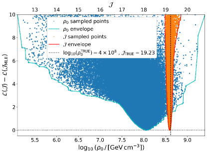
Figure 1: Comparison between fitting $\rho_{0}$ or $\mathcal{J}$ – together with the other parameters in Eq. 9 – in the analysis of a mock stellar kinematic data-set. The blue (orange) points represent the likelihood evaluations projected onto the $\rho_{0}$ ($\mathcal{J}$) direction of the parameter space. The cyan (red) curve indicates the envelope of the sampled points along $\rho_{0}$ ($\mathcal{J})$. The vertical dashed line corresponds to the true value of $\rho_{0}$ and correspondingly $\mathcal{J}$.

The advantage of performing an inference on $\mathcal{J}$, rather than $\rho_{0}$, is manifest in Fig. 1. This figure displays the likelihood evaluations (Eq. 3) obtained leaving either $\rho_{0}$ (blue points) or $\mathcal{J}$ (orange points) free – along with the other parameters of Eq. 9 – in the analysis of a (simulated) stellar kinematic data-set. We note how the envelope of the former points (cyan curve) is much broader than the envelope of the latter (red curve). This difference shows how the reparameterisation in Eq. 11 considerably mitigates the degeneracy between the DM normalisation parameter and the nuisance parameters. Moreover, we also observe how the likelihood sampling with respect to $\rho_{0}$ seems to be biased towards small values of this quantity. Importantly, we note that for finite MCMC sampling steps, the $J$-envelope of the likelihood evaluations will inevitably be a non-smooth curve. To remedy this feature, and contextually optimise the statistical bias and coverage, we parameterise the envelope of the likelihood with

$$h(x;p,q,r)=e^{-p\,x}+q\,x+r\,,$$ (13)

where $p,q,r$ are free parameters and $x=\mathcal{J}-\mathcal{J}_{\textrm{MLE}}$. The equation above represents an adaptation of the Linex loss function (Chang & Hung, 2007) and its application on Draco is shown in Fig. 2 (solid blue line). Comparing this curve with Fig. 1 of CH17 (dashed grey line), we see how varying even the DM profile shape parameters in the fit leads to a broadening of the profile likelihood. Additionally, we include the likelihood adopted by Ackermann et al. (2015, dot-dashed brown line). We emphasise that this curve was obtained by fitting a log-normal to a posterior probability sampled with the Multi-level Bayesian modelling (MLM) proposed by Martinez (2015). This aspect highlights the importance of determining $J$-factor likelihoods in a consistent manner. To determine the robustness of a this method, we assess its statistical performance on a simulation suite. The details of the tests are presented in the next section.

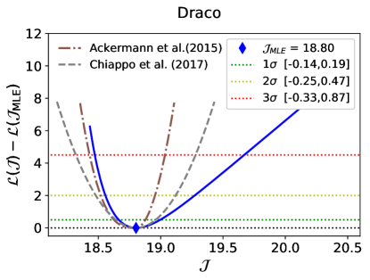
Figure 2: Profile likelihood of $\mathcal{J}$ for Draco dSph. The solid blue curve is obtained by approximating the result of the $J$-sampling technique (the envelope) with Eq. 13. We analyse the kinematic data assuming isotropic stellar velocities, with spatial distribution following a Plummer profile. For the DM component, a generalised NFW is adopted, all parameters of which are free in the optimisation (see text). For reference, the analogous result obtained by CH17 is also shown (dashed gray line), together with the curve used by Ackermann et al. (2015) (dot-dashed brown line).

3 Validation on Gaia simulations

We validate our method on the publicly available simulation suite released by Gaia Challenge (Walker & Peñarrubia, 2011, hereafter GAIASIM) . The manual-profiling approach was already tested by CH17 using the same mock data. Since those authors considered a more restrictive (simplified) model, the expectation for the current, more general study is that the same tests would lead to larger bias and higher statistical coverage. These predictions are motivated by the freedom in the likelihood, on one side, and by its flatness in $J$ due to the indeterminacy of some nuisance parameters, on the other.

Table 1: Models tested with the $J$-sampling MLE scheme. For each, we optimise the likelihood in Eq. 3 using data-sets containing $N_{\star}=100,200,500,1000$. All models assume $r_{0}$ = 1 kpc. The entries in the fifth column ($c_{\star}$) refer to the inner slope of the Hernquist profile (Eq. 9) describing the stellar distribution.

Mock dSph data-sets	$\rho_{0}$ ($\text{M}_{\odot}\text{kpc}^{-3}$)	$\mathcal{J}_{\textrm{TRUE}}$	$r_{a}$ (kpc)	$c_{\star}$	$r_{\star}$ (kpc)
OM Core non-Plummer	4$\times 10^{8}$	19.23	0.25	1	0.25
OM Core Plummer-like	4$\times 10^{8}$	19.23	0.25	0.1	0.25
Isotropic Core non-Plummer	4$\times 10^{8}$	19.23	$\infty$	1	1
Isotropic Core Plummer-like	4$\times 10^{8}$	19.23	$\infty$	0.1	1
OM Cusp non-Plummer	6.4$\times 10^{7}$	18.83	0.1	1	0.1
OM Cusp Plummer-like	6.4$\times 10^{7}$	18.83	0.1	0.1	0.1
Isotropic Cusp non-Plummer	6.4$\times 10^{7}$	18.83	$\infty$	1	0.25
Isotropic Cusp Plummer-like	6.4$\times 10^{7}$	18.83	$\infty$	0.1	0.25

Here we assess the $J$-sampling approach by repeating the tests performed by CH17 on the eight models listed in Table 1. In line with the modelling assumptions described above (Sec. 2), we consider only the single-component models released by GAIASIM and analysed by CH17. When fitting each mock data-set, we assume the true model in Eq. 4, with the exception of $\rho_{\textrm{DM}}$. For the DM profile, a generalised NFW (Eq. 9) is adopted, but its shape parameters are free to vary. This means that the MCMC tool samples a total of 5 (6) parameters, namely $\mathcal{J},r_{0},a,b,c$ (plus $r_{a}$), whose allowed ranges are listed in Table 2.

Table 2: Parameters ranges allowed in all fits performed in this project.

$\mathcal{J}$	$\in$	$[10,30]$
$\log_{10}(r_{0}/1\,\textrm{kpc})$	$\in$	$[-3,2]$
$\log_{10}(r_{a}/1\,\textrm{kpc})$	$\in$	$[-3,2]$
$\beta$	$\in$	$[-9,0.9]$
$a$	$\in$	$(0,8]$
$b$	$\in$	$[0.5,10]$
$c$	$\in$	$[0,1.5)$

In order to validate the statistical properties of the method, we estimate its bias and the statistical coverage of the 1,2,3$\sigma$ intervals. Similarly to CH17, we do this for samples of different sizes, obtained by partitioning the full data-set – the one containing $10^{4}$ stars – into non-overlapping subsets of 100,200,500,1000 stars. For instance, this operation produces $N_{\textrm{PE}}$ = 50 (20) mock samples or pseudo-experiments (PE) containing $N_{\star}$ = 200 (500) stars.

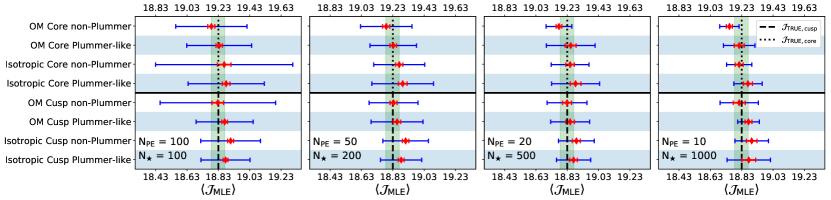
Figure 3: Bias estimates of the frequentist fitting method implemented via the $J$-sampling scheme. In every panel, the red points represent the mean of the $\mathcal{J}_{\textrm{MLE}}$ estimates, obtained from the approximation with Eq.13 of the likelihood resulting from the analysis of each PE. The blue (red) error bars correspond to the root mean square (uncertainty on the mean) of the MLE values, while the vertical dashed (dotted) line indicates the true $\mathcal{J}$ for the Cusp (Core) models (see Table 1). The vertical green band gives the $\mathcal{J}$ range where the bias in $J$ is $\leq$ 10%.

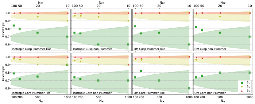
Figure 4: Coverage probability as a function of the sample size. In every panel, the green squares, the yellow downward triangles and the red upward triangles indicate, respectively, the statistical coverage of the 1,2,3$\sigma$ intervals. The coloured bands represent the ranges of expected statistical coverage of an ideal experiment, corresponding to each $\sigma$ level. This means that the green, yellow and red areas are centred, respectively, on 68%, 95% and 99%, and widen with decreasing $N_{\textrm{PE}}$ (see text). Every panel in this figure refers to one of the eight Gaia models considered here (see Table 1), as indicated in the bottom-left corner of each plot.

The outcome of these tests is shown in Figs. 3 and 4, displaying the bias and statistical coverage, respectively. All results reported in these figures were obtained by approximating the $\mathcal{J}$-envelope with Eq. 13. The statistical coverage is generally high or within the expected range (coloured bands in Fig. 4). The occurrence of marginal under-coverage (at the 3$\sigma$ level in the Isotropic Core non-Plummer model) is plausibly a symptom of the low statistics regime ($N_{\textrm{PE}}=10$). Importantly, we observe an increase of the bias for the $N_{\star}=100$ and 1000 cases, as compared to the analogous result by CH17 (their Fig. 5). This feature is likely a reflection of the indeterminacy of some parameters mentioned above. Moreover, we recall that the MLE of a quantity becomes an unbiased estimator only asymptotically (James, 2006). Whereas the uncertainty on $\left<\mathcal{J}_{\mathrm{MLE}}\right>$ is generally small (red error bars in Fig. 3), we note a large scatter in the estimates (blue error bars in the same figure), which reduces with growing $N_{\star}$. This feature is consistent with the expectations from the validation of a frequentist approach. Finally, it should be remembered, as noted by CH17, that the GAIASIM simulations were not generated from a Gaussian velocity distribution. Therefore, fitting the mock kinematic data with a Gaussian likelihood entails a model systematics, which could be potentially responsible for the observed bias.

Altogether, the results reported in this section indicate that the method possesses satisfactory statistical properties for the $N_{\star}$ range considered. We verified using the same mock data that the both bias and statistical coverage increase significantly when analysing smaller data-sets. This aspect supports the suitability of this procedure only for large kinematic samples. This conclusion necessarily imposes restrictions for the application on real stellar data, as detailed in the next section.

4 Results on real kinematic data

Table 3: Properties of the MW dSphs considered in this work. Values taken from Albert et al. (2017) and McConnachie (2012).

Name	$l,b$	Distance	$r_{1/2}$	$M_{V}$	$N_{\star}$
	(deg, deg)	(kpc)	(pc)	(mag)
Canes Venatici I	$74.31,79.82$	218	441	$-8.6$	214
Carina	$260.11,-22.22$	105	205	$-9.1$	758
Draco	$86.37,34.72$	76	184	$-8.8$	353
Fornax	$237.10,-65.65$	147	594	$-13.4$	2409
Leo I	$225.99,49.11$	254	223	$-12.0$	328
Leo II	$220.17,67.23$	233	164	$-9.8$	175
Sagittarius	$5.6,-14.2$	26	400	$-13.5$	1373
Sculptor	$287.53,-83.16$	86	233	$-11.1$	1352
Sextans	$243.50,42.27$	86	561	$-9.3$	424
Ursa Minor	$104.97,44.80$	76	120	$-8.8$	196

Having explored the statistical properties of our frequentist $J$-sampling method, we proceed to applying it on data from real dSphs. To comply with the considerations presented above (Sec. 3), we consider the dSphs with the most abundant kinematic sample available in the literature (McConnachie, 2012), which results in ten galaxies with $N_{\star}\geq 100$. The systems and their properties are summarised in Table 3. In order to facilitate the comparison between our estimates and results in the literature, we always use $\Delta\Omega=2.4\times 10^{-4}$ sr, equivalent to $\theta_{\textrm{max}}=0.5^{\circ}$. In accordance with the validation presented above, the profile likelihood curve for every dSph is built by approximating with Eq. 13 the output of the $J$-sampling approach (see Sec. 2). The fit of each kinematic sample is repeated three times, implementing the ISO (Eq. 5a), OM (Eq. 5b) and CB (Eq. 5c) kernel functions, respectively. We assume throughout a Plummer profile for the stellar density and a generalised NFW (Eq. 9) for the DM distribution. Therefore, the likelihood is sampled over the 5-(6-)dimensional parameter space $\mathcal{J},r_{0},a,b,c$ (plus $r_{a}$ or $\beta$). The results are shown collectively in Fig. 5, which displays the best-fit $\mathcal{J}$ values, together with their uncertainty in the form of error bars reflecting the 1$\sigma$ confidence interval. The output of our method (circles) is compared with that of CH17 (squares), when adopting the ISO (red),the OM (green) and the CB (blue) models. We also include recent Bayesian-derived estimates used by Ackermann et al. (2015, upward black triangles) and those obtained by Geringer-Sameth et al. (2015c, downward black triangles) and by Bonnivard et al. (2015a, black circles). Our results are also listed in Table 4, together with the best estimates of the parameter values of Eq. 13. The full likelihoods corresponding to the data entering Fig. 5 are shown in Fig. 9 in the Appendix.

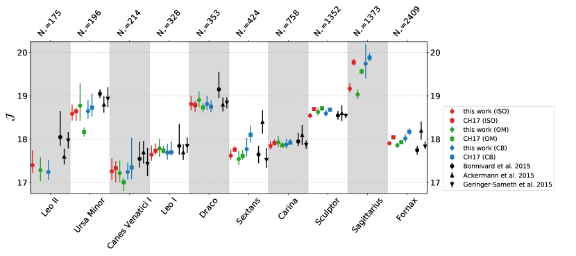
Figure 5: Best-fit $\mathcal{J}$ values from the analysis of stellar kinematic data from 10 dSphs. The estimates are obtained from the approximation with Eq. 13 of the $\mathcal{J}$-envelope, constructed with the $J$-sampling scheme (circles). In all cases we assume a Plummer profile for the stellar brightness and a generalised NFW (Eq. 9) for the DM profile. The red, green and blue symbols refer to the cases where we adopt the isotropic, OM and constant-$\beta$ velocity kernel functions, respectively. For comparison, the analogous values released by CH17 are included (squares). The black points represent previous Bayesian-derived results used by Ackermann et al. (2015, upward triangles) and obtained by Geringer-Sameth et al. (2015c, downward triangles) and Bonnivard et al. (2016, circles). The uncertainties on the estimates correspond to the 1$\sigma$ confidence intervals.

In most cases, the $\mathcal{J}_{\textrm{MLE}}$ values we obtain are consistent with the other sets of results, within quoted uncertainties. Although they use an analogous (frequentist) method, CH17 considered a less flexible model whereby they fixed the shape parameters in Eq. 9 to the NFW case. Despite assuming similar parameter ranges, the fitting methodology adopted by Geringer-Sameth et al. (2015c) differs substantially from our. In their work, these authors implemented MultiNest (Feroz et al., 2013) to explore a 6-dimensional parameter space. Hence, the Geringer-Sameth et al. (2015c) estimates of the $\rho_{\textrm{DM}}$ parameters are influenced by the prior probability density. Although Ackermann et al. (2015) examined a larger dimensionality parameters space, this does not match the one considered here. In particular, Ackermann et al. (2015) don’t fit the parameters of the profiles entering Eq. 4. Instead, those authors infer prior ranges on two characteristics of DM halos ($v_{\textrm{max}},r_{\textrm{max}}$) by assuming several (fixed) parametrisations of $\rho_{\textrm{DM}}$ (see Martinez 2015 for details). Moreover, the same authors acknowledge the significant effect of prior choices on the marginalised posterior probability of $\mathcal{J}$ they derive (see Fig. 1 of Martinez 2015).

Table 4: Tabulated values of the $\mathcal{J}_{\textrm{MLE}}$ estimates entering Fig. 5. Columns 4,5,6 (8,9,10) [12,13,14] contain the best-fit parameters of the Eq. 13 approximating the $\mathcal{J}$-envelope, in turn obtained from the $J$-sampling scheme when assuming an ISO (OM) [CB] velocity anisotropy model.

Dwarf	$N_{\star}$	$\mathcal{J}_{\textrm{MLE}}$ (ISO)	$p$	$q$	$r$	$\mathcal{J}_{\textrm{MLE}}$ (OM)	$p$	$q$	$r$	$\mathcal{J}_{\textrm{MLE}}$ (CB)	$p$	$q$	$r$
Leo II	175	${17.40}^{+0.35}_{-0.18}$	$7.23$	$2.38$	$-0.09$	${17.29}^{+0.30}_{-0.25}$	$2.31$	$5.80$	$-0.45$	${17.24}^{+0.28}_{-0.17}$	$4.98$	$4.25$	$-1.02$
Ursa Minor	196	${18.58}^{+0.21}_{-0.16}$	$4.66$	$6.47$	$-0.99$	${18.77}^{+0.51}_{-0.34}$	$2.96$	$2.00$	$-0.86$	${18.65}^{+0.26}_{-0.17}$	$4.06$	$5.57$	$-1.02$
Canes Venatici I	214	${17.26}^{+0.30}_{-0.19}$	$5.51$	$3.33$	$-1.07$	${17.22}^{+0.29}_{-0.21}$	$4.77$	$3.66$	$-1.05$	${17.25}^{+0.21}_{-0.18}$	$5.18$	$5.51$	$-1.01$
Leo I	328	${17.64}^{+0.21}_{-0.14}$	$5.32$	$6.45$	$-1.31$	${17.79}^{+0.22}_{-0.19}$	$2.82$	$8.44$	$-0.60$	${17.69}^{+0.20}_{-0.16}$	$4.19$	$7.40$	$-1.21$
Draco	353	${18.81}^{+0.19}_{-0.15}$	$5.89$	$6.45$	$-1.02$	${18.90}^{+0.20}_{-0.16}$	$3.63$	$8.45$	$-1.11$	${18.81}^{+0.19}_{-0.14}$	$6.29$	$6.27$	$-1.07$
Sextans	424	${17.62}^{+0.14}_{-0.09}$	$7.52$	$10.50$	$-0.79$	${17.54}^{+0.18}_{-0.14}$	$5.26$	$7.75$	$-0.97$	${17.77}^{+0.26}_{-0.17}$	$6.98$	$3.44$	$-1.08$
Carina	758	${17.84}^{+0.10}_{-0.08}$	$11.82$	$10.74$	$-0.77$	${17.93}^{+0.15}_{-0.10}$	$6.62$	$10.29$	$-1.20$	${17.88}^{+0.14}_{-0.09}$	$11.57$	$7.41$	$-1.02$
Sculptor	1352	${18.54}^{+0.06}_{-0.04}$	$16.74$	$22.11$	$-1.03$	${18.63}^{+0.10}_{-0.08}$	$9.48$	$13.21$	$-1.82$	${18.59}^{+0.08}_{-0.07}$	$13.61$	$13.48$	$-1.23$
Sagittarius	1373	${19.16}^{+0.13}_{-0.09}$	$9.78$	$9.50$	$-0.84$	${19.03}^{+0.11}_{-0.10}$	$7.01$	$12.39$	$-1.29$	${19.74}^{+0.44}_{-0.34}$	$1.90$	$3.58$	$-0.87$
Fornax	2409	${17.91}^{+0.05}_{-0.04}$	$22.70$	$19.47$	$-0.77$	${17.86}^{+0.06}_{-0.05}$	$14.67$	$22.05$	$-1.22$	${18.02}^{+0.10}_{-0.09}$	$9.36$	$13.08$	$-1.67$

We stress that our statistical approach (profile likelihood for frequentist $J$-factors) is not dependent on the model assumptions, and thus is easily extendable to other systems, such as faint dSphs, once more kinematic data is provided. Moreover, this procedure can be applied to all galaxies where spectroscopic observations are available, e.g. field galaxies or their satellite galaxies. However, in the former case the modelling might change, with the spherical Jeans equation likely not being warranted any more. Additionally, the contribution of stars to the gravitational potential would need to be incorporated in the model. In this situation, the use of the Jeans formalism should possibly be abandoned, in favour of a physically motivated velocity distribution function. The derivation of this quantity and its implementation in the frequentist schemes presented here is currently under development and will be presented in a future publication.

5 Consistent Dark Matter annihilation cross-section limits

In this section we implement the profile likelihoods of $\mathcal{J}$ with the $\gamma$-ray data, for the latter using the Fermi-LAT observations, producing consistent DM annihilation cross-section limits. We use all curves derived in Sec. 4, with the exception of Sagittarius. This dSph is the closest to the MW (Table 3) and is known to be experiencing strong tidal disruption by the MW potential (Johnston et al., 1995). Similarly, most previous analyses of $\gamma$-ray data neglect this system when searching for possible signals of annihilating DM in dSphs of the Local Group (Ackermann et al., 2015; Drlica-Wagner et al., 2015a; Albert et al., 2017).

It is customary in astronomy to compare an observed photon flux with the expectations via a Poisson likelihood. Clearly, in doing so, the contamination from concomitant spurious sources, such as the galactic diffuse emission and point sources, must be adequately taken into account. Performing this subtraction for the LAT data entails an analysis using the Fermi Science Tools . Conveniently, Ackermann et al. (2015) have published their results in the form of bin-by-bin likelihood tables (see Ackermann et al. 2015 and reference therein for more details). Inference of DM properties proceeds then via the optimisation of the following function (Ackermann et al., 2015)

$$\mathcal{L}_{\textrm{d}}(\bm{\mu},\bm{\Xi}=(\bm{\alpha},J_{\textrm{d}})|\mathcal{D^{\textrm{d}}}=(\mathcal{D}^{\textrm{d}}_{\gamma},\mathcal{D}^{\textrm{d}}_{\star}))=$$

$$-\ln P_{\textrm{d}}(\bm{\mu},\bm{\alpha},J_{\textrm{d}}|\mathcal{D}^{\textrm{d}}_{\gamma})\,+\mathcal{L}_{J}(J_{\textrm{d}}|\mathcal{D}^{\textrm{d}}_{\star})\,.$$ (14)

In Eq. 14, the vector $\bm{\mu}$ represents the parameters of interest $(m_{\textrm{DM}},\left<\sigma v\right>)$, while $\bm{\Xi}$ contains the nuisance parameters involved in the Poisson likelihood ($P$) optimisation, $\bm{\alpha}$, and the $J$-factor. $\mathcal{D}^{\textrm{d}}$ comprises the photon data, $\mathcal{D}^{\textrm{d}}_{\gamma}$, and the stellar kinematic sample, $\mathcal{D}^{\textrm{d}}_{\star}$. The index ’d’, appearing in most terms of Eq. 14, indicates that these quantities refer to a specific dSph. Since the properties of a given DM candidate are assumed to be invariant across different targets, it is possible to combine the likelihood for each dSph (Eq. 14) into a unique object. Optimising the following joint likelihood (Ackermann et al., 2011)

$$\widetilde{\mathcal{L}}(\bm{\mu})=\prod^{N_{\textrm{dwarfs}}}_{\textrm{d=1}}\mathcal{L}_{\textrm{d}}(\bm{\mu},\bm{\Xi}|\mathcal{D}^{\textrm{d}})\,,$$ (15)

thus increases the sensitivity over individual targets. From Eq. 14 we see that $\mathcal{L}_{J}(J)$ plays a decisive role in the determination of the DM particle properties. Optimising this formula with respect to $J$ allows the propagation of astrophysical uncertainties when constraining $\left<\sigma v\right>$. The importance of using a frequentist-derived $J$-factor likelihood in Eq. 14 is displayed in Fig. 6. This figure compares the $J$-envelope (red curve) of the likelihood evaluations (orange dots) with the marginalisation of the same over all nuisance parameters (blue histogram). We note how both the profiled (red curve) and marginalised (black curve) likelihoods recover well the true $J$-factor. However, the marginalisation process produces a narrower curve than the former, especially at large $\mathcal{J}$ values. This feature implies that uncertainties obtained from the marginalised posterior are artificially smaller than what indicated by the profile likelihood.

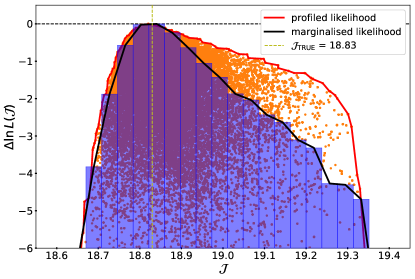
Figure 6: Comparison between profiling and marginalising the likelihood over the nuisance parameters. The orange points indicate the likelihood evaluations over the allowed parameter space. The marginalisation of these points gives the blue histogram. The different width of the $J$-envelope (red curve) and the marginalised likelihood (black curve) at large $\mathcal{J}$ displays the effect on the uncertainties on the parameter yielded by the two statistical approaches. The stellar kinematic data used when sampling the likelihood belongs to one of the PE analysed in Sec. 3. The vertical dashed line indicates the true value of $\mathcal{J}$ for the underlying GAIASIM model.

Setting limits on the DM annihilation cross-section with $\widetilde{\mathcal{L}}$ entails, for a fixed $m_{\textrm{DM}}$, finding the largest value of $\left<\sigma v\right>$ for which $\widetilde{\mathcal{L}}$ increases by $2.71/2$ from its minimum. Repeating this process for a range of a masses yields a curve in the $(m_{\textrm{DM}},\left<\sigma v\right>)$ plane, which provides a 95% confidence level upper limit (UL) on $\left<\sigma v\right>$. The product of this operation is reported in Fig. 7, where our result (blue solid curve) is displayed together with the analogous one calculated implementing the $J$ likelihood parameterisations proposed by Ackermann et al. (2011, red dot-dashed curve) and Ackermann et al. (2015, green dashed curve). We reiterate that the $J$ likelihood curves adopted in these works were obtained via Bayesian analyses of stellar kinematic data, implementing flat priors in the former and the MLM priors of Martinez (2015) in the latter. Therefore, Fig. 7 provides a direct comparison of the UL on $\left<\sigma v\right>$ stemming from the different statistical configurations. The dSphs sample chosen for the three joint likelihood analyses is dictated by the set of targets considered in Ackermann et al. (2011) and Ackermann et al. (2015): for consistency, we select the subset of dSphs common to both publications. We are, thus, left with the following systems: Carina, Draco, Fornax, Sculptor, Sextans and Ursa Minor. For illustrative reasons, we assume that all DM annihilates into $W^{+}W^{-}$ pairs. Unsurprisingly, the UL derived from the flat-prior $J$ likelihoods is very similar to that calculated with our profile likelihood curves of $J$. This resemblance follows the observation that our likelihood sampling expedient is, essentially, an ordinary MCMC where the priors are deprived of their numerical influence on the likelihood. Moreover, the targets sample considered contains the brightest known dSphs of the MW and Bayesian statistics progressively becomes less sensitive to priors as the number of observations grows. Following the previous point, the stronger constraining power of the MLM UL (shown in green) is principally determined by the action of the MLM priors in the (Bayesian) analysis of the kinematic data by Martinez (2015). Importantly, Fig. 7 elucidates the advantage of performing a frequentist analysis of stellar data over the standard Bayesian framework: removing the effect of priors, we eliminate their influence on the DM annihilation cross-section ULs, associated with the arbitrariness of their selection.

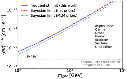
Figure 7: DM annihilation cross-section 95 per cent upper limits from a combined analysis of six dSphs (see figure) using $J$-factor likelihoods derived with different statistical assumptions. The blue solid curve represents the new, consistent UL determined by implementing the $\mathcal{L}(\mathcal{J})$ curves derived with the frequentist method presented in this work (Sec. 2). For comparison, the dot-dashed red (dashed green) line constitutes the analogous result calculated with the $J$-factor likelihood parameterisation adopted by Ackermann et al. 2011 (Ackermann et al. 2015). The curves are obtained assuming that all DM annihilates through the $W^{+}W^{-}$ channel. The dotted grey curve is the thermal relic cross section derived in Steigman et al. (2012).

The frequentist UL shown in Fig. 7 is calculated adopting the likelihood curves of $J$ derived in the isotropic stellar velocities assumption. This choice guarantees the modelling consistency underlying the $J$ likelihood component of the UL determination entering the figure. The effect of implementing different velocity anisotropy models on the DM annihilation ULs is portrayed in Fig. 8.

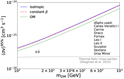
Figure 8: Same as Fig. 7, but obtained considering nine dSphs (see figure) and using $J$-factor likelihoods built by implementing different models of the stellar velocity anisotropy. Specifically, we consider the case of isotropic velocities (solid blue line), constant degree of anisotropy $\beta$ (dot-dashed red line) and the OM profile (dashed green line). The curves are derived assuming that all DM annihilates into $b\bar{b}$ quarks. The dotted grey curve represents the thermal relic cross section derived in Steigman et al. (2012).

In producing this plot, we consider a broader sample of dSphs, consisting of all systems listed in Table 4 except Sagittarius, due to the arguments presented at the beginning of this section. Moreover, we assume that all DM annihilates into $b\bar{b}$ quark pairs, when the stellar velocities are isotropically oriented (Eq. 5a, solid blue line), when they have a constant degree of anisotropy throughout the dSphs (Eq. 5b, dot-dashed red line) or have an OM radial velocity anisotropy profile (Eq. 5c, dashed green line). The similarity of these curves is driven by the affinity of the corresponding $J$ likelihood curves for most dSphs considered – shown in Fig. 9 in the Appendix – and the proximity of their $\mathcal{J}_{\textrm{MLE}}$ values, especially.

6 Conclusion

The high energy radiation from dSphs may be the key to DM indirect identification. Undesirably, the inaccessibility of the spatial distribution of DM within dSphs undermines current searches by introducing a major source of systematic uncertainty. Some of this indeterminacy has been typically tamed by means of Bayesian techniques. Inevitably, though, the presence of priors in this kind of analysis entails potential bias on the estimates, in this case the MLE $J$-factor. Moreover, the optimisation of Eq. 14 with respect to $J$ implies the propagation of the effect of priors to the final result: the DM annihilation $\left<\sigma v\right>^{95\%}$ UL. Since the Poisson likelihood in Eq. 14 is usually obtained in a frequentist manner, the use of such Bayesian-derived $J$-factor likelihoods entails an inconsistency in the statistical approach employed to derive the $\left<\sigma v\right>^{95\%}$ UL.

Adopting the reformulation of $J$ proposed by CH17 (Eq. 11), with an expedient for using the MCMC within a frequentist framework, we devise a scheme for fitting a generalised Jeans equation to the stellar kinematics of a dSph, removing the need for priors. The validation of our method on simulations (Sec. 3) indicates that this frequentist approach possesses satisfactory statistical properties, when analysing sufficiently large kinematic samples (i.e. for $N_{\star}\geq 100$). Following this prescription, we obtain new, prior-free profile likelihoods for the $J$-factor of 10 bright dSphs. The MLE values of $J$ we derive are broadly consistent with previous results found in the literature.

Implementing the new likelihood curves in the optimisation of Eq. 15, provides the first statistically-consistent (fully-frequentist) ULs on the DM annihilation cross-section. From multiple joint-likelihood analyses of six dSphs, we compare the new constraints with those obtained implementing the (Bayesian-derived) parameterisations of the likelihood of $J$ proposed by Ackermann et al. (2011, using flat priors) and Ackermann et al. (2015, involving MLM priors). An advantage of our method is the removal of the potential arbitrariness related to the choice of priors. Additionally, we present $\left<\sigma v\right>^{95\%}$ ULs on the DM annihilation associated with different assumptions on the velocity anisotropy of the stellar population of dSphs. The similarity of the constraints (and $J$-factors – see Fig. 9) for the different models considered in this work (Eq. 5c) could be due to the mass-anisotropy degeneracy afflicting the mass determination in dSphs (Wolf et al., 2010).

A possible venue of improvement of this method concerns the use of a Gaussian likelihood for the los velocities of stars (Eq. 3). This ad-hoc assumption could be replaced, for example, by adopting 3-dimensional Gaussian stellar velocities, as done in the MAMPOSSt routine (Mamon et al., 2013). Alternatively, the dynamics of stars in dSphs can be modelled via action-angle variables, as done in the AGAMA code (Vasiliev, 2019); for a recent review on the topic, see Sanders & Binney (2016). The solution that we intend to pursue in the future entails the derivation of the physical velocity distribution function of the system from the Eddington inversion formula (Binney & Tremaine, 2008). We note that this calculation can be performed only for the stellar velocity anisotropy models considered here (Binney & Tremaine, 2008). Recent applications of this technique to the stellar population of the MW have proven to reproduce quite accurately the observations (Piffl et al., 2014; Binney & Sanders, 2014; Sharma et al., 2014). Moreover, the use of the Gaussian approximation may be the culprit for the sub-optimal statistical properties of the profile likelihood resulting from the fitting schemes presented in Section 2. We also note that the performance of the method can be improved by implementing an exponential cut-off in the DM distribution, as done in previous works (see Łokas et al. 2005 and references therein). However, we take the effect of this modification – which mimics the tidal stripping by the potential of the Milky Way (Kazantzidis et al., 2004) – to be incorporated into the approximation with Eq. 13 (see Sec. 2). Generally, our method depends on the availability of abundant kinematic samples, ideally extending to large projected radial distances. This assertion implies that the analysis of ultra-faint dSphs will inevitably necessitate more spectroscopic observations. Extensive stellar data for these systems will allow to implement a joint-likelihood analysis for a broader ensemble of targets, thereby setting new, data-driven ULs on $\left<\sigma v\right>$. Additionally, we will be able to compare the frequentist constraints with the Bayesian ones (for example of Ackermann et al. 2015) and test the claimed detection of $\gamma$ rays in Ret II dSph (Geringer-Sameth et al., 2015b). We, therefore, auspicate that future surveys will perform accurate and extended spectroscopic observations of ultra-faint and newly discovered dSphs, for example those recently detected by the DES observatory (Bechtol et al., 2015; Drlica-Wagner et al., 2015b).

Appendix A Profile likelihood curves

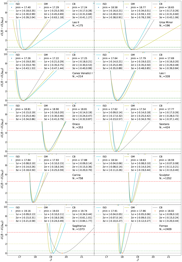
Figure 9: Full likelihoods for the ten dSphs considered in this work. Each panel refers to a given system, as indicated in the images. The curves shown represent the approximation with Eq. 13 of the likelihood resulting from the $J$-sampling scheme when implementing the isotropic (cyan line), OM (olive line) and constant-$\beta$ (grey line) velocity anisotropy models. The best-fit $\mathcal{J}$ values and the width of the 1,2,3$\sigma$ intervals are also indicated in each panel, for each curve.

References

- Ackermann et al. (2011) Ackermann M., et al., 2011, Phys. Rev. Lett., 107, 241302
- Ackermann et al. (2015) Ackermann M., et al., 2015, Phys. Rev. Lett., 115, 231301
- Ahnen et al. (2016) Ahnen M. L., et al., 2016, JCAP, 1602, 039
- Albert et al. (2017) Albert A., et al., 2017, ApJ, 834, 110
- Baltz et al. (2000) Baltz E. A., Briot C., Salati P., Taillet R., Silk J., 2000, Phys. Rev. D, 61, 023514
- Battaglia et al. (2006) Battaglia G., et al., 2006, A&A, 459, 423
- Battaglia et al. (2013) Battaglia G., Helmi A., Breddels M., 2013, New Astron. Rev., 57, 52
- Bechtol et al. (2015) Bechtol K., et al., 2015, ApJ, 807, 50
- Bergstrom (2000) Bergstrom L., 2000, Rept. Prog. Phys., 63, 793
- Bertone et al. (2005) Bertone G., Hooper D., Silk J., 2005, Phys. Rept., 405, 279
- Binney & Mamon (1982) Binney J., Mamon G. A., 1982, MNRAS, 200, 361
- Binney & Sanders (2014) Binney J., Sanders J. L., 2014, in Feltzing S., Zhao G., Walton N. A., Whitelock P., eds, IAU Symposium Vol. 298, Setting the scene for Gaia and LAMOST. pp 117–129 (arXiv:1309.2790), doi:10.1017/S1743921313006297
- Binney & Tremaine (1987) Binney J., Tremaine S., 1987, Galactic dynamics. Princeton series of astrophysics
- Binney & Tremaine (2008) Binney J., Tremaine S., 2008, Galactic Dynamics: Second Edition. Princeton University Press
- Bonnivard et al. (2015a) Bonnivard V., Combet C., Maurin D., Walker M. G., 2015a, MNRAS, 446, 3002
- Bonnivard et al. (2015b) Bonnivard V., et al., 2015b, ApJ, 808, L36
- Bonnivard et al. (2016) Bonnivard V., Hütten M., Nezri E., Charbonnier A., Combet C., Maurin D., 2016, Comput. Phys. Commun., 200, 336
- Chang & Hung (2007) Chang Y.-c., Hung W.-l., 2007, Quality & Quantity, 41, 291
- Charles et al. (2016) Charles E., et al., 2016, Phys. Rept., 636, 1
- Chiappo et al. (2017) Chiappo A., Cohen-Tanugi J., Conrad J., Strigari L. E., Anderson B., Sanchez-Conde M. A., 2017, MNRAS, 466, 669
- Conrad (2014) Conrad J., 2014, Astropart. Phys., 62, 165
- Conrad et al. (2015) Conrad J., Cohen-Tanugi J., Strigari L. E., 2015, J. Exp. Theor. Phys., 121, 1104
- Drlica-Wagner et al. (2015a) Drlica-Wagner A., et al., 2015a, ApJ, 809, L4
- Drlica-Wagner et al. (2015b) Drlica-Wagner A., et al., 2015b, ApJ, 813, 109
- Feroz et al. (2013) Feroz F., Hobson M. P., Cameron E., Pettitt A. N., 2013
- Foreman-Mackey et al. (2013) Foreman-Mackey D., Hogg D. W., Lang D., Goodman J., 2013, PASP, 125, 306
- Gaskins (2016) Gaskins J. M., 2016, Contemp. Phys., 57, 496
- Geringer-Sameth et al. (2015a) Geringer-Sameth A., Koushiappas S. M., Walker M. G., 2015a, Phys. Rev. D, 91, 083535
- Geringer-Sameth et al. (2015b) Geringer-Sameth A., Walker M. G., Koushiappas S. M., Koposov S. E., Belokurov V., Torrealba G., Evans N. W., 2015b, Phys. Rev. Lett., 115, 081101
- Geringer-Sameth et al. (2015c) Geringer-Sameth A., Koushiappas S. M., Walker M., 2015c, ApJ, 801, 74
- James (2006) James F., 2006, Statistical methods in experimental physics
- Johnston et al. (1995) Johnston K. V., Spergel D. N., Hernquist L., 1995, ApJ, 451, 598
- Kazantzidis et al. (2004) Kazantzidis S., Magorrian J., Moore B., 2004, ApJ, 601, 37
- Kormendy & Freeman (2016) Kormendy J., Freeman K. C., 2016, ApJ, 817, 84
- Kuhlen et al. (2009) Kuhlen M., Madau P., Silk J., 2009, Science, 325, 970
- Łokas et al. (2005) Łokas E. L., Mamon G. A., Prada F., 2005, MNRAS, 363, 918
- Mamon & Łokas (2005) Mamon G. A., Łokas E. L., 2005, MNRAS, 363, 705
- Mamon & Łokas (2006) Mamon G. A., Łokas E. L., 2006, MNRAS, 370, 1582
- Mamon et al. (2013) Mamon G. A., Biviano A., Boué G., 2013, MNRAS, 429, 3079
- Martinez (2015) Martinez G. D., 2015, MNRAS, 451, 2524
- McConnachie (2012) McConnachie A. W., 2012, AJ, 144, 4
- Merritt (1985) Merritt D., 1985, AJ, 90, 1027
- Morå (2015) Morå K., 2015, in 27th Rencontres de Blois on Particle Physics and Cosmology Blois, France, May 31-June 5, 2015. (arXiv:1512.00698), https://inspirehep.net/record/1407811/files/arXiv:1512.00698.pdf
- Osipkov (1979) Osipkov L. P., 1979, Soviet Astronomy Letters, 5, 42
- Piffl et al. (2014) Piffl T., et al., 2014, MNRAS, 445, 3133
- Plummer (1911) Plummer H. C., 1911, MNRAS, 71, 460
- Sanders & Binney (2016) Sanders J. L., Binney J., 2016, MNRAS, 457, 2107
- Sharma et al. (2014) Sharma S., et al., 2014, ApJ, 793, 51
- Simon et al. (2011) Simon J. D., et al., 2011, ApJ, 733, 46
- Springel et al. (2008) Springel V., et al., 2008, MNRAS, 391, 1685
- Steigman et al. (2012) Steigman G., Dasgupta B., Beacom J. F., 2012, Phys. Rev. D, D86, 023506
- Vasiliev (2019) Vasiliev E., 2019, MNRAS, 482, 1525
- Walker & Peñarrubia (2011) Walker M. G., Peñarrubia J., 2011, ApJ, 742, 20
- Wilks (1938) Wilks S. S., 1938, Annals Math. Statist., 9, 60
- Wolf et al. (2010) Wolf J., Martinez G. D., Bullock J. S., Kaplinghat M., Geha M., Munoz R. R., Simon J. D., Avedo F. F., 2010, MNRAS, 406, 1220
- Wood et al. (2015) Wood M., Anderson B., Drlica-Wagner A., Cohen-Tanugi J., Conrad J., 2015, in Proceedings, 34th International Cosmic Ray Conference (ICRC 2015). (arXiv:1507.03530), http://inspirehep.net/record/1382564/files/arXiv:1507.03530.pdf
- Zhao (1996) Zhao H., 1996, MNRAS, 278, 488
- Zitzer (2015a) Zitzer B., 2015a, in Proceedings, 34th International Cosmic Ray Conference (ICRC 2015). (arXiv:1509.01105), https://inspirehep.net/record/1391628/files/arXiv:1509.01105.pdf
- Zitzer (2015b) Zitzer B., 2015b, in Fifth International Fermi Symposium Nagoya, Japan, October 20-24, 2014. (arXiv:1503.00743), https://inspirehep.net/record/1347106/files/arXiv:1503.00743.pdf