On fractional annealing process
Tran Manh Tuong
University of Finance and Marketing, Ho Chi Minh City, VietNam
email:tmtuong@ufm.edu.vn
Tran Hung Thao
Institute of Mathematics, Vietnam Academy of Science and Technology
thaoth@math.ac.vn
Abstract
The paper deals with a full annealing process, for example for a metal alloy perturbed by some fractional noise caused by conditions in furnace such as initial temperature, initial structure of material itself, β¦The energy of the heating matter system depending on its states at each time, we consider some steady state at full annealing range by introducing a fractional model for it. And we determine states of the system related to this steady state.
keywords:
fractional annealing, steady state,
L 2 β limit-from superscript πΏ 2 L^{2}- approximation
β β journal: Journal of La Te X Β Templates
1 Introduction
As we know, full anneal is a special stage of annealing process where a condensed matter (a steel for example) is heated to slightly above the critical temperature (name austenitic temperature) and maintaining the temperature for a special period of time to allow the material to fully form austenite or austenite cementite grain structure (see [1], [2], [4], [6]).
Denote by X t β ( t β₯ 0 ) , X t β β d subscript π π‘ π‘ 0 subscript π π‘
superscript β π X_{t}(t\geq 0),X_{t}\in\mathbb{R}^{d} , a stochastic process presenting the state of the material under full annealing stage at time t π‘ t and g β ( X t ) π subscript π π‘ g(X_{t}) is the system energy corresponding to state X t subscript π π‘ X_{t} , where g π g is a Borel function on β n superscript β π \mathbb{R}^{n} .
It is well-know that a classical stochastic model for annealing states X t subscript π π‘ X_{t} is given by the following equation:
d X t = β β½ g ( X t ) d t + 2 β T d W t dX_{t}=-\bigtriangledown g(X_{t})dt+\sqrt{2T}dW_{t}
(1.1)
where W t subscript π π‘ W_{t} is a d β limit-from π d- dimensional Brownian motion expressing a no-memory noise and T π T is the temperature of the system (see [3]). In our context T π T can be considered unchange as it is the austenitic temperature.
A problem is that full annealing treatments should be made in batch-type furnaces that are in full compliance of temperature uniformity and accuracy requirements of pyrometry AMS2750. In such type of furnace, the system state ( X t , t β₯ 0 ) subscript π π‘ π‘
0 (X_{t},t\geq 0) is no more no-memory process because each value of X t subscript π π‘ X_{t} at t π‘ t can influence upon its values some times after t π‘ t . Therefore the model (1.1) is no more suitable. And we propose the following model
d X t = β β½ g ( X t ) d t + 2 β T d B t H dX_{t}=-\bigtriangledown g(X_{t})dt+\sqrt{2T}dB^{H}_{t}
(1.2)
where:
1.
B t H subscript superscript π΅ π» π‘ B^{H}_{t} is a d β limit-from π d- dimensional fractional Brownian motion of Liouvill form
B t H = ( B t H j , j = 1 , 2 , β¦ , d ) , B t H j = β« 0 t ( t β s ) H j β 1 / 2 β π W s j , j = 1 , 2 , β¦ , d \begin{split}B^{H}_{t}&=(B^{H_{j}}_{t},j=1,2,\dots,d),\\
B^{H_{j}}_{t}&=\int_{0}^{t}(t-s)^{H_{j}-1/2}dW^{j}_{s},j=1,2,\dots,d\end{split}
2.
H j subscript π» π H_{j} are Hurst parameters, 0 < H j < 1 0 subscript π» π 1 0<H_{j}<1 .
3.
W t j subscript superscript π π π‘ W^{j}_{t} are standard Brownian motion.
4.
g = g β ( x 1 , β¦ , x d ) π π subscript π₯ 1 β¦ subscript π₯ π g=g(x_{1},\dots,x_{d}) is a Borel function β d β β β superscript β π β \mathbb{R}^{d}\to\mathbb{R} and g β C 1 β ( β d ) π superscript πΆ 1 superscript β π g\in C^{1}(\mathbb{R}^{d}) .
The state process ( X t ) subscript π π‘ (X_{t}) satisfying the equation (1.2) driven by the perturbation B t H subscript superscript π΅ π» π‘ B^{H}_{t} is a process with memory as expected.
But (1.2) is a fractional stochastic differential equation and its solution can not be found by means of traditional stochastic calculus as we can made for the equation (1.2). Many approaches have been introduced to overcome this difficulty for such kind of equation. And one of these approaches is given by Thao T.H via an approximation method. This method is presented briefly in Section 2 below.
Now let X β = ( X 1 β , X 2 β , β¦ , X d β ) superscript π subscript superscript π 1 subscript superscript π 2 β¦ subscript superscript π π X^{*}=(X^{*}_{1},X^{*}_{2},\dots,X^{*}_{d}) be a steady state on the full annealing range that means β g β x i β ( X β ) = 0 , i = 1 , 2 , β¦ , d formulae-sequence π subscript π₯ π superscript π 0 π 1 2 β¦ π
\frac{\partial g}{\partial x_{i}}(X^{*})=0,i=1,2,\dots,d . In this note we try to find the relation between a state process satisfying (1.2) and the steady state X β superscript π X^{*} .
2 Fractional Brownian motion and an approximation approach
Now we recall some facts of one-dimensional fractional Brownian motion in Mandelbrot form ([7]-[10]). It is a centered Gaussian process W t H subscript superscript π π» π‘ W^{H}_{t} such that its covariance function is given by
R β ( t , s ) = 1 2 β ( t 2 β H + s 2 β H β | t β s | 2 β H ) , 0 < H < 1 formulae-sequence π
π‘ π 1 2 superscript π‘ 2 π» superscript π 2 π» superscript π‘ π 2 π» 0 π» 1 R(t,s)=\frac{1}{2}(t^{2H}+s^{2H}-\mathinner{\!\left\lvert t-s\right\rvert}^{2H}),0<H<1
(2.1)
If H = 1 / 2 , R β ( t , s ) = min β‘ ( t , s ) formulae-sequence π» 1 2 π
π‘ π π‘ π H=1/2,R(t,s)=\min(t,s) and W t H subscript superscript π π» π‘ W^{H}_{t} is an usual standard Brownian motion.
If H β 1 / 2 , W t H π» 1 2 subscript superscript π π» π‘
H\neq 1/2,W^{H}_{t} is a process of long memory, and Ito calculus cannot applied to it. And an approximation approach is given as follows ([7]).
It is known that W t H subscript superscript π π» π‘ W^{H}_{t} can be decomposed as
W t H = 1 Ξ β ( Ξ± + 1 ) β [ Z t + β« 0 t ( t β s ) Ξ± β π W s ] , Ξ± = H β 1 / 2 formulae-sequence subscript superscript π π» π‘ 1 Ξ πΌ 1 delimited-[] subscript π π‘ superscript subscript 0 π‘ superscript π‘ π πΌ differential-d subscript π π πΌ π» 1 2 W^{H}_{t}=\frac{1}{\Gamma(\alpha+1)}\left[Z_{t}+\int_{0}^{t}(t-s)^{\alpha}dW_{s}\right],\alpha=H-1/2
where Z t subscript π π‘ Z_{t} is a process having absolutely continuous paths and the long memory property focus at the term
B t H = β« 0 t ( t β s ) Ξ± β π W s , Ξ± = H β 1 / 2 formulae-sequence subscript superscript π΅ π» π‘ superscript subscript 0 π‘ superscript π‘ π πΌ differential-d subscript π π πΌ π» 1 2 B^{H}_{t}=\int_{0}^{t}(t-s)^{\alpha}dW_{s},\alpha=H-1/2
which is called the fractional Brownian motion of the Liouville form.
Since B t H subscript superscript π΅ π» π‘ B^{H}_{t} is not a semimartingale we introduce a new process for each Ο΅ > 0 italic-Ο΅ 0 \epsilon>0
B t H , Ο΅ = β« 0 t ( t β s + Ο΅ ) Ξ± β π W s subscript superscript π΅ π» italic-Ο΅
π‘ superscript subscript 0 π‘ superscript π‘ π italic-Ο΅ πΌ differential-d subscript π π B^{H,\epsilon}_{t}=\int_{0}^{t}(t-s+\epsilon)^{\alpha}dW_{s}
And the following two important facts have been proved in [7] and [10].
1.
B t H , Ο΅ subscript superscript π΅ π» italic-Ο΅
π‘ B^{H,\epsilon}_{t} is a semimartingale:
d β B H , Ο΅ = Ξ± β Ο t Ο΅ β d β t + Ο΅ Ξ± β d β W t π superscript π΅ π» italic-Ο΅
πΌ subscript superscript π italic-Ο΅ π‘ π π‘ superscript italic-Ο΅ πΌ π subscript π π‘ dB^{H,\epsilon}=\alpha\varphi^{\epsilon}_{t}dt+\epsilon^{\alpha}dW_{t}
where
Ο t Ο΅ = β« 0 t ( t β s + Ο΅ ) Ξ± β 1 β π W s superscript subscript π π‘ italic-Ο΅ superscript subscript 0 π‘ superscript π‘ π italic-Ο΅ πΌ 1 differential-d subscript π π \varphi_{t}^{\epsilon}=\int_{0}^{t}(t-s+\epsilon)^{\alpha-1}dW_{s}
2.
B t H , Ο΅ subscript superscript π΅ π» italic-Ο΅
π‘ B^{H,\epsilon}_{t} converges to B t H subscript superscript π΅ π» π‘ B^{H}_{t} in L 2 β ( Ξ© ) superscript πΏ 2 Ξ© L^{2}(\Omega) as Ο΅ italic-Ο΅ \epsilon tends to 0. And this convergence is uniform with respect to t π‘ t belong to any finite interval I πΌ I of time, and we have also
sup t β I β₯ B t H , Ο΅ β B t H β₯ β€ C β ( Ξ± ) β Ο΅ 2 β H subscript supremum π‘ πΌ delimited-β₯β₯ subscript superscript π΅ π» italic-Ο΅
π‘ subscript superscript π΅ π» π‘ πΆ πΌ superscript italic-Ο΅ 2 π» \sup_{t\in I}\mathinner{\!\left\lVert B^{H,\epsilon}_{t}-B^{H}_{t}\right\rVert}\leq C(\alpha)\epsilon^{2H}
where C β ( Ξ± ) πΆ πΌ C(\alpha) is a positive constant depending only to Ξ± = H β 1 / 2 πΌ π» 1 2 \alpha=H-1/2 .
Apart from this, a study of fractional stochastic differential equations is presented in [8], [9] and [10].
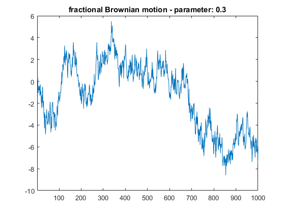
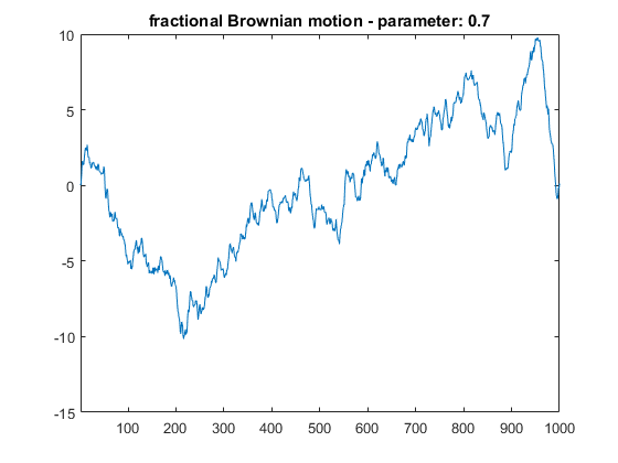
Fractional Brownian motion with H =0.3 and d = 1
Fractional Brownian motion with H =0.7 and d = 1
3 Fractional annealing process
For the sake of the simplicity we consider the case of two dimensions d = 2 π 2 d=2 . The case of general dimension d π d can be naturally extended. So we are supposed to consider the following model
d X t = β β½ g ( X t ) d t + 2 β T d B t H dX_{t}=-\bigtriangledown g(X_{t})dt+\sqrt{2T}dB^{H}_{t}
where
X t = ( X t 1 X t 2 ) , g = g β ( x 1 , x 2 ) , B t H = ( B t H 1 B t H 2 ) formulae-sequence subscript π π‘ matrix subscript superscript π 1 π‘ subscript superscript π 2 π‘ formulae-sequence π π subscript π₯ 1 subscript π₯ 2 subscript superscript π΅ π» π‘ matrix subscript superscript π΅ subscript π» 1 π‘ subscript superscript π΅ subscript π» 2 π‘ X_{t}=\begin{pmatrix}X^{1}_{t}\\
X^{2}_{t}\end{pmatrix},g=g(x_{1},x_{2}),B^{H}_{t}=\begin{pmatrix}B^{H_{1}}_{t}\\
B^{H_{2}}_{t}\end{pmatrix}
B t H j = β« 0 t ( t β s ) Ξ± j β π W j , Ξ± j = H j β 1 / 2 , 0 < H j < 1 , j = 1 , 2 formulae-sequence formulae-sequence subscript superscript π΅ subscript π» π π‘ superscript subscript 0 π‘ superscript π‘ π subscript πΌ π differential-d subscript π π formulae-sequence subscript πΌ π subscript π» π 1 2 0 subscript π» π 1 π 1 2
B^{H_{j}}_{t}=\int_{0}^{t}(t-s)^{\alpha_{j}}dW_{j},\alpha_{j}=H_{j}-1/2,0<H_{j}<1,j=1,2
Let X β = ( X 1 β , X 2 β ) superscript π superscript subscript π 1 superscript subscript π 2 X^{*}=(X_{1}^{*},X_{2}^{*}) be a steady state on full annealing range where β g β x 1 β ( X β ) = 0 , β g β x 2 β ( X β ) = 0 formulae-sequence π subscript π₯ 1 superscript π 0 π subscript π₯ 2 superscript π 0 \frac{\partial g}{\partial x_{1}}(X^{*})=0,\frac{\partial g}{\partial x_{2}}(X^{*})=0 . We have to calculate state satisfying (1.6) and relating to X β superscript π X^{*} .
3.1 A change of variables
Denote by F 1 β ( x 1 , x 2 ) subscript πΉ 1 subscript π₯ 1 subscript π₯ 2 F_{1}(x_{1},x_{2}) and F 2 β ( x 1 , x 2 ) subscript πΉ 2 subscript π₯ 1 subscript π₯ 2 F_{2}(x_{1},x_{2}) be the partial derivatives of g β ( x 1 , x 2 ) π subscript π₯ 1 subscript π₯ 2 g(x_{1},x_{2}) :
F 1 β ( x ) = F 1 β ( x 1 , x 2 ) = β β β x 1 β g β ( x 1 , x 2 ) F 2 β ( x ) = F 2 β ( x 1 , x 2 ) = β β β x 2 β g β ( x 1 , x 2 ) matrix subscript πΉ 1 π₯ subscript πΉ 1 subscript π₯ 1 subscript π₯ 2 subscript π₯ 1 π subscript π₯ 1 subscript π₯ 2 subscript πΉ 2 π₯ subscript πΉ 2 subscript π₯ 1 subscript π₯ 2 subscript π₯ 2 π subscript π₯ 1 subscript π₯ 2 \begin{matrix}F_{1}(x)=F_{1}(x_{1},x_{2})=-\frac{\partial}{\partial x_{1}}g(x_{1},x_{2})\\
F_{2}(x)=F_{2}(x_{1},x_{2})=-\frac{\partial}{\partial x_{2}}g(x_{1},x_{2})\end{matrix}
and
F β ( x ) = ( F 1 β ( x ) F 2 β ( x ) ) πΉ π₯ matrix subscript πΉ 1 π₯ subscript πΉ 2 π₯ F(x)=\begin{pmatrix}F_{1}(x)\\
F_{2}(x)\end{pmatrix}
The equation (1.2) can be rewritten as following
d β X t = F β ( X t ) β d β t + 2 β T β d β B t H π subscript π π‘ πΉ subscript π π‘ π π‘ 2 π π subscript superscript π΅ π» π‘ dX_{t}=F(X_{t})dt+\sqrt{2T}dB^{H}_{t}
or
{ d β X t 1 = F 1 β ( X t ) β d β t + 2 β T β d β B t H 1 d β X t 2 = F 2 β ( X t ) β d β t + 2 β T β d β B t H 2 cases π superscript subscript π π‘ 1 subscript πΉ 1 subscript π π‘ π π‘ 2 π π subscript superscript π΅ subscript π» 1 π‘ otherwise π superscript subscript π π‘ 2 subscript πΉ 2 subscript π π‘ π π‘ 2 π π subscript superscript π΅ subscript π» 2 π‘ otherwise \begin{cases}dX_{t}^{1}=F_{1}(X_{t})dt+\sqrt{2T}dB^{H_{1}}_{t}\\
dX_{t}^{2}=F_{2}(X_{t})dt+\sqrt{2T}dB^{H_{2}}_{t}\end{cases}
We have now
F 1 β ( X β ) = 0 β Β andΒ β F 2 β ( X β ) = 0 subscript πΉ 1 superscript π 0 Β andΒ subscript πΉ 2 superscript π 0 F_{1}(X^{*})=0\text{ and }F_{2}(X^{*})=0
Define a change of variable
X t = ( X t 1 X t 2 ) β U t = ( U t 1 U t 2 ) = X t β X β = ( X t 1 β X 1 β£ β X t 2 β X 2 β£ β ) subscript π π‘ matrix subscript superscript π 1 π‘ subscript superscript π 2 π‘ β subscript π π‘ matrix subscript superscript π 1 π‘ subscript superscript π 2 π‘ subscript π π‘ superscript π matrix subscript superscript π 1 π‘ superscript π 1
subscript superscript π 2 π‘ superscript π 2
X_{t}=\begin{pmatrix}X^{1}_{t}\\
X^{2}_{t}\end{pmatrix}\to U_{t}=\begin{pmatrix}U^{1}_{t}\\
U^{2}_{t}\end{pmatrix}=X_{t}-X^{*}=\begin{pmatrix}X^{1}_{t}-X^{1*}\\
X^{2}_{t}-X^{2*}\end{pmatrix}
We can see that
( d β U t 1 d β U t 2 ) = ( β F 1 β x 1 β ( X β ) β F 1 β x 2 β ( X β ) β F 1 β x 2 β ( X β ) β F 2 β x 2 β ( X β ) ) β ( U t 1 U t 2 ) β d β t + 2 β T β ( d β B t H 1 d β B t H 2 ) matrix π subscript superscript π 1 π‘ π subscript superscript π 2 π‘ matrix subscript πΉ 1 subscript π₯ 1 superscript π subscript πΉ 1 subscript π₯ 2 superscript π subscript πΉ 1 subscript π₯ 2 superscript π subscript πΉ 2 subscript π₯ 2 superscript π matrix subscript superscript π 1 π‘ subscript superscript π 2 π‘ π π‘ 2 π matrix π subscript superscript π΅ subscript π» 1 π‘ π subscript superscript π΅ subscript π» 2 π‘ \begin{pmatrix}dU^{1}_{t}\\
dU^{2}_{t}\end{pmatrix}=\begin{pmatrix}\frac{\partial F_{1}}{\partial x_{1}}(X^{*})&\frac{\partial F_{1}}{\partial x_{2}}(X^{*})\\
\frac{\partial F_{1}}{\partial x_{2}}(X^{*})&\frac{\partial F_{2}}{\partial x_{2}}(X^{*})\end{pmatrix}\begin{pmatrix}U^{1}_{t}\\
U^{2}_{t}\end{pmatrix}dt+\sqrt{2T}\begin{pmatrix}dB^{H_{1}}_{t}\\
dB^{H_{2}}_{t}\end{pmatrix}
or
d β U t = A β U t β d β t + 2 β T β d β B t H π subscript π π‘ π΄ subscript π π‘ π π‘ 2 π π subscript superscript π΅ π» π‘ dU_{t}=AU_{t}dt+\sqrt{2T}dB^{H}_{t}
where
A = ( a 1 b 1 a 2 b 2 ) : = ( β F 1 β x 1 β ( X β ) β F 1 β x 2 β ( X β ) β F 1 β x 2 β ( X β ) β F 2 β x 2 β ( X β ) ) A=\begin{pmatrix}a_{1}&b_{1}\\
a_{2}&b_{2}\end{pmatrix}\mathrel{\mathop{\mathchar 58\relax}}=\begin{pmatrix}\frac{\partial F_{1}}{\partial x_{1}}(X^{*})&\frac{\partial F_{1}}{\partial x_{2}}(X^{*})\\
\frac{\partial F_{1}}{\partial x_{2}}(X^{*})&\frac{\partial F_{2}}{\partial x_{2}}(X^{*})\end{pmatrix}
Then we can write (3.1.3) as follows
{ d β U t 1 = ( a 1 β U t 1 + b 1 β U t 2 ) β d β t + 2 β T β d β B t H 1 d β U t 2 = ( a 2 β U t 1 + b 2 β U t 2 ) β d β t + 2 β T β d β B t H 2 cases π subscript superscript π 1 π‘ subscript π 1 subscript superscript π 1 π‘ subscript π 1 subscript superscript π 2 π‘ π π‘ 2 π π subscript superscript π΅ subscript π» 1 π‘ otherwise π subscript superscript π 2 π‘ subscript π 2 subscript superscript π 1 π‘ subscript π 2 subscript superscript π 2 π‘ π π‘ 2 π π subscript superscript π΅ subscript π» 2 π‘ otherwise \begin{cases}dU^{1}_{t}=(a_{1}U^{1}_{t}+b_{1}U^{2}_{t})dt+\sqrt{2T}dB^{H_{1}}_{t}\\
dU^{2}_{t}=(a_{2}U^{1}_{t}+b_{2}U^{2}_{t})dt+\sqrt{2T}dB^{H_{2}}_{t}\end{cases}
3.2 Approximate model
Now we can consider an approximate model corresponding to (3.1.4) or (3.1.6) by replacing B t H = ( B t H 1 B t H 2 ) subscript superscript π΅ π» π‘ matrix subscript superscript π΅ subscript π» 1 π‘ subscript superscript π΅ subscript π» 2 π‘ B^{H}_{t}=\begin{pmatrix}B^{H_{1}}_{t}\\
B^{H_{2}}_{t}\end{pmatrix} by B t H , Ο΅ = ( B t H 1 , Ο΅ 1 B t H 2 , Ο΅ 2 ) subscript superscript π΅ π» italic-Ο΅
π‘ matrix subscript superscript π΅ subscript π» 1 subscript italic-Ο΅ 1
π‘ subscript superscript π΅ subscript π» 2 subscript italic-Ο΅ 2
π‘ B^{H,\epsilon}_{t}=\begin{pmatrix}B^{H_{1},\epsilon_{1}}_{t}\\
B^{H_{2},\epsilon_{2}}_{t}\end{pmatrix} as introduced in section 1.
d β U t Ο΅ = A β U t Ο΅ β d β t + 2 β T β d β B t H , Ο΅ π subscript superscript π italic-Ο΅ π‘ π΄ subscript superscript π italic-Ο΅ π‘ π π‘ 2 π π subscript superscript π΅ π» italic-Ο΅
π‘ dU^{\epsilon}_{t}=AU^{\epsilon}_{t}dt+\sqrt{2T}dB^{H,\epsilon}_{t}
and
{ d β U t 1 , Ο΅ 1 = ( a 1 β U t 1 , Ο΅ 1 + b 1 β U t 2 , Ο΅ 2 ) β d β t + 2 β T β d β B t H 1 , Ο΅ 1 d β U t 2 , Ο΅ 2 = ( a 2 β U t 1 , Ο΅ 1 + b 2 β U t 2 , Ο΅ 2 ) β d β t + 2 β T β d β B t H 2 , Ο΅ 2 cases π subscript superscript π 1 subscript italic-Ο΅ 1
π‘ subscript π 1 subscript superscript π 1 subscript italic-Ο΅ 1
π‘ subscript π 1 subscript superscript π 2 subscript italic-Ο΅ 2
π‘ π π‘ 2 π π subscript superscript π΅ subscript π» 1 subscript italic-Ο΅ 1
π‘ otherwise π subscript superscript π 2 subscript italic-Ο΅ 2
π‘ subscript π 2 subscript superscript π 1 subscript italic-Ο΅ 1
π‘ subscript π 2 subscript superscript π 2 subscript italic-Ο΅ 2
π‘ π π‘ 2 π π subscript superscript π΅ subscript π» 2 subscript italic-Ο΅ 2
π‘ otherwise \begin{cases}dU^{1,\epsilon_{1}}_{t}=(a_{1}U^{1,\epsilon_{1}}_{t}+b_{1}U^{2,\epsilon_{2}}_{t})dt+\sqrt{2T}dB^{H_{1},\epsilon_{1}}_{t}\\
dU^{2,\epsilon_{2}}_{t}=(a_{2}U^{1,\epsilon_{1}}_{t}+b_{2}U^{2,\epsilon_{2}}_{t})dt+\sqrt{2T}dB^{H_{2},\epsilon_{2}}_{t}\end{cases}
where B t H j , Ο΅ j β B t H j β subscript superscript π΅ subscript π» π subscript italic-Ο΅ π
π‘ subscript superscript π΅ subscript π» π π‘ B^{H_{j},\epsilon_{j}}_{t}\to B^{H_{j}}_{t} in the space L 2 = L 2 β ( Ξ© ) superscript πΏ 2 superscript πΏ 2 Ξ© L^{2}=L^{2}(\Omega) of square integrable processes, and
β₯ B t H j , Ο΅ j β B t H j β₯ L 2 β€ C j β ( Ξ± j ) β Ο΅ j 2 β H j , Ξ± j = H j β 1 / 2 , j = 1 , 2 formulae-sequence subscript delimited-β₯β₯ subscript superscript π΅ subscript π» π subscript italic-Ο΅ π
π‘ subscript superscript π΅ subscript π» π π‘ superscript πΏ 2 subscript πΆ π subscript πΌ π superscript subscript italic-Ο΅ π 2 subscript π» π formulae-sequence subscript πΌ π subscript π» π 1 2 π 1 2
\mathinner{\!\left\lVert B^{H_{j},\epsilon_{j}}_{t}-B^{H_{j}}_{t}\right\rVert}_{L^{2}}\leq C_{j}(\alpha_{j})\epsilon_{j}^{2H_{j}},\alpha_{j}=H_{j}-1/2,j=1,2
with C β ( Ξ± j ) πΆ subscript πΌ π C(\alpha_{j}) depending only on Ξ± j subscript πΌ π \alpha_{j} (see [7]).
3.3 Convergence
Before finding the solution U t Ο΅ subscript superscript π italic-Ο΅ π‘ U^{\epsilon}_{t} of (3.2.1) we will prove a convergence theorem.
Theorem 3.1
The solution U t Ο΅ subscript superscript π italic-Ο΅ π‘ U^{\epsilon}_{t} of (3.2.1) tend to the solution U t subscript π π‘ U_{t} of (2.7) in L 2 superscript πΏ 2 L^{2} as Ο΅ β 0 β italic-Ο΅ 0 \epsilon\to 0 , that means
U t 1 , Ο΅ 1 β U t 1 β Β inΒ β L 2 β Β asΒ β Ο΅ 1 β 0 β subscript superscript π 1 subscript italic-Ο΅ 1
π‘ subscript superscript π 1 π‘ Β inΒ superscript πΏ 2 Β asΒ subscript italic-Ο΅ 1 β 0 U^{1,\epsilon_{1}}_{t}\to U^{1}_{t}\text{ in }L^{2}\text{ as }\epsilon_{1}\to 0
and
U t 2 , Ο΅ 2 β U t 2 β Β inΒ β L 2 β Β asΒ β Ο΅ 2 β 0 β subscript superscript π 2 subscript italic-Ο΅ 2
π‘ subscript superscript π 2 π‘ Β inΒ superscript πΏ 2 Β asΒ subscript italic-Ο΅ 2 β 0 U^{2,\epsilon_{2}}_{t}\to U^{2}_{t}\text{ in }L^{2}\text{ as }\epsilon_{2}\to 0
Proof 1
We have
U t 1 β U t 1 , Ο΅ 1 = β« 0 t [ a 1 β ( U t 1 β U 1 , Ο΅ 1 ) + b 1 β ( U t 2 β U t 2 , Ο΅ 2 ) ] β π s + 2 β T β ( B t H 1 β B t H 1 , Ο΅ 1 ) subscript superscript π 1 π‘ subscript superscript π 1 subscript italic-Ο΅ 1
π‘ superscript subscript 0 π‘ delimited-[] subscript π 1 subscript superscript π 1 π‘ superscript π 1 subscript italic-Ο΅ 1
subscript π 1 subscript superscript π 2 π‘ subscript superscript π 2 subscript italic-Ο΅ 2
π‘ differential-d π 2 π subscript superscript π΅ subscript π» 1 π‘ subscript superscript π΅ subscript π» 1 subscript italic-Ο΅ 1
π‘ U^{1}_{t}-U^{1,\epsilon_{1}}_{t}=\int_{0}^{t}\left[a_{1}(U^{1}_{t}-U^{1,\epsilon_{1}})+b_{1}(U^{2}_{t}-U^{2,\epsilon_{2}}_{t})\right]ds+\sqrt{2T}(B^{H_{1}}_{t}-B^{H_{1},\epsilon_{1}}_{t})
U t 2 β U t 2 , Ο΅ 2 = β« 0 t [ a 2 β ( U t 1 β U 1 , Ο΅ 1 ) + b 2 β ( U t 2 β U t 2 , Ο΅ 2 ) ] β π s + 2 β T β ( B t H 2 β B t H 2 , Ο΅ 2 ) subscript superscript π 2 π‘ subscript superscript π 2 subscript italic-Ο΅ 2
π‘ superscript subscript 0 π‘ delimited-[] subscript π 2 subscript superscript π 1 π‘ superscript π 1 subscript italic-Ο΅ 1
subscript π 2 subscript superscript π 2 π‘ subscript superscript π 2 subscript italic-Ο΅ 2
π‘ differential-d π 2 π subscript superscript π΅ subscript π» 2 π‘ subscript superscript π΅ subscript π» 2 subscript italic-Ο΅ 2
π‘ U^{2}_{t}-U^{2,\epsilon_{2}}_{t}=\int_{0}^{t}\left[a_{2}(U^{1}_{t}-U^{1,\epsilon_{1}})+b_{2}(U^{2}_{t}-U^{2,\epsilon_{2}}_{t})\right]ds+\sqrt{2T}(B^{H_{2}}_{t}-B^{H_{2},\epsilon_{2}}_{t})
Put M = max β‘ ( | a 1 | 2 , | a 2 | 2 , | b 1 | 2 , | b 2 | 2 ) π subscript π 1 2 subscript π 2 2 subscript π 1 2 subscript π 2 2 M=\max\left(\frac{\mathinner{\!\left\lvert a_{1}\right\rvert}}{2},\frac{\mathinner{\!\left\lvert a_{2}\right\rvert}}{2},\frac{\mathinner{\!\left\lvert b_{1}\right\rvert}}{2},\frac{\mathinner{\!\left\lvert b_{2}\right\rvert}}{2}\right) . Then it follows from (3.3.1), (3.3.2) and (2.5) that
β₯ U t 1 β U t 1 , Ο΅ 1 β₯ + β₯ U t 2 β U t 2 , Ο΅ 2 β₯ β€ C β ( Ξ± , Ο΅ ) + M β β« 0 1 [ β₯ U s 1 β U s 1 , Ο΅ 1 β₯ + β₯ U t 2 β U t 2 , Ο΅ 2 β₯ ] β π s delimited-β₯β₯ subscript superscript π 1 π‘ subscript superscript π 1 subscript italic-Ο΅ 1
π‘ delimited-β₯β₯ subscript superscript π 2 π‘ subscript superscript π 2 subscript italic-Ο΅ 2
π‘ πΆ πΌ italic-Ο΅ π superscript subscript 0 1 delimited-[] delimited-β₯β₯ subscript superscript π 1 π subscript superscript π 1 subscript italic-Ο΅ 1
π delimited-β₯β₯ subscript superscript π 2 π‘ subscript superscript π 2 subscript italic-Ο΅ 2
π‘ differential-d π \mathinner{\!\left\lVert U^{1}_{t}-U^{1,\epsilon_{1}}_{t}\right\rVert}+\mathinner{\!\left\lVert U^{2}_{t}-U^{2,\epsilon_{2}}_{t}\right\rVert}\leq C(\alpha,\epsilon)+M\int_{0}^{1}\left[\mathinner{\!\left\lVert U^{1}_{s}-U^{1,\epsilon_{1}}_{s}\right\rVert}+\mathinner{\!\left\lVert U^{2}_{t}-U^{2,\epsilon_{2}}_{t}\right\rVert}\right]ds
where
C β ( Ξ± , Ο΅ ) = 2 β T β ( C 1 β ( Ξ± 1 ) β Ο΅ 1 1 + 2 β Ξ± 1 + C 2 β ( Ξ± 2 ) β Ο΅ 2 1 + 2 β Ξ± 2 ) β 0 πΆ πΌ italic-Ο΅ 2 π subscript πΆ 1 subscript πΌ 1 superscript subscript italic-Ο΅ 1 1 2 subscript πΌ 1 subscript πΆ 2 subscript πΌ 2 superscript subscript italic-Ο΅ 2 1 2 subscript πΌ 2 β 0 C(\alpha,\epsilon)=\sqrt{2T}\left(C_{1}(\alpha_{1})\epsilon_{1}^{1+2\alpha_{1}}+C_{2}(\alpha_{2})\epsilon_{2}^{1+2\alpha_{2}}\right)\to 0
as Ο΅ = ( Ο΅ 1 , Ο΅ 2 ) β 0 italic-Ο΅ subscript italic-Ο΅ 1 subscript italic-Ο΅ 2 β 0 \epsilon=(\epsilon_{1},\epsilon_{2})\to 0
Then an application of Gronwall inequality gives us
β₯ U t 1 β U t 1 , Ο΅ 1 β₯ + β₯ U t 2 β U t 2 , Ο΅ 2 β₯ β€ C β ( Ξ± , Ο΅ ) β exp β‘ ( M β t ) β 0 delimited-β₯β₯ subscript superscript π 1 π‘ subscript superscript π 1 subscript italic-Ο΅ 1
π‘ delimited-β₯β₯ subscript superscript π 2 π‘ subscript superscript π 2 subscript italic-Ο΅ 2
π‘ πΆ πΌ italic-Ο΅ π π‘ β 0 \mathinner{\!\left\lVert U^{1}_{t}-U^{1,\epsilon_{1}}_{t}\right\rVert}+\mathinner{\!\left\lVert U^{2}_{t}-U^{2,\epsilon_{2}}_{t}\right\rVert}\leq C(\alpha,\epsilon)\exp{(Mt)}\to 0
as Ο΅ β 0 β italic-Ο΅ 0 \epsilon\to 0 . So that
U t Ο΅ = ( U t 1 , Ο΅ 1 U t 2 , Ο΅ 2 ) β ( U t 1 U t 2 ) = U t β Β inΒ β L 2 β Β asΒ β Ο΅ = ( Ο΅ 1 , Ο΅ 2 ) β 0 subscript superscript π italic-Ο΅ π‘ matrix subscript superscript π 1 subscript italic-Ο΅ 1
π‘ subscript superscript π 2 subscript italic-Ο΅ 2
π‘ β matrix subscript superscript π 1 π‘ subscript superscript π 2 π‘ subscript π π‘ Β inΒ superscript πΏ 2 Β asΒ italic-Ο΅ subscript italic-Ο΅ 1 subscript italic-Ο΅ 2 β 0 U^{\epsilon}_{t}=\begin{pmatrix}U^{1,\epsilon_{1}}_{t}\\
U^{2,\epsilon_{2}}_{t}\end{pmatrix}\to\begin{pmatrix}U^{1}_{t}\\
U^{2}_{t}\end{pmatrix}=U_{t}\text{ in }L^{2}\text{ as }\epsilon=(\epsilon_{1},\epsilon_{2})\to 0
3.4 Solution U t Ο΅ subscript superscript π italic-Ο΅ π‘ U^{\epsilon}_{t} of (3.2.1)
Now we have to find the solution of U t Ο΅ subscript superscript π italic-Ο΅ π‘ U^{\epsilon}_{t} in its explicit form. We have
d β U t Ο΅ = A β U t Ο΅ β d β t + 2 β T β d β B t H , Ο΅ π subscript superscript π italic-Ο΅ π‘ π΄ subscript superscript π italic-Ο΅ π‘ π π‘ 2 π π subscript superscript π΅ π» italic-Ο΅
π‘ dU^{\epsilon}_{t}=AU^{\epsilon}_{t}dt+\sqrt{2T}dB^{H,\epsilon}_{t}
where
A = ( a 1 b 1 a 2 b 2 ) , U t Ο΅ = ( U t H 1 , Ο΅ 1 U t H 2 , Ο΅ 2 ) , B t Ο΅ = ( B t H 1 , Ο΅ 1 B t H 2 , Ο΅ 2 ) formulae-sequence π΄ matrix subscript π 1 subscript π 1 subscript π 2 subscript π 2 formulae-sequence subscript superscript π italic-Ο΅ π‘ matrix subscript superscript π subscript π» 1 subscript italic-Ο΅ 1
π‘ subscript superscript π subscript π» 2 subscript italic-Ο΅ 2
π‘ subscript superscript π΅ italic-Ο΅ π‘ matrix subscript superscript π΅ subscript π» 1 subscript italic-Ο΅ 1
π‘ subscript superscript π΅ subscript π» 2 subscript italic-Ο΅ 2
π‘ A=\begin{pmatrix}a_{1}&b_{1}\\
a_{2}&b_{2}\end{pmatrix},U^{\epsilon}_{t}=\begin{pmatrix}U^{H_{1},\epsilon_{1}}_{t}\\
U^{H_{2},\epsilon_{2}}_{t}\end{pmatrix},B^{\epsilon}_{t}=\begin{pmatrix}B^{H_{1},\epsilon_{1}}_{t}\\
B^{H_{2},\epsilon_{2}}_{t}\end{pmatrix}
It is easy to see that
U t Ο΅ = β« 0 t e A β ( t β s ) β 2 β T β π B t H , Ο΅ subscript superscript π italic-Ο΅ π‘ superscript subscript 0 π‘ superscript π π΄ π‘ π 2 π differential-d subscript superscript π΅ π» italic-Ο΅
π‘ U^{\epsilon}_{t}=\int_{0}^{t}e^{A(t-s)}\sqrt{2T}dB^{H,\epsilon}_{t}
A method by Oksendal can be applied ([6], page 99) to obtain
e A β ( t β s ) = e β Ξ» β ( t β s ) ΞΎ β [ ΞΎ β cos β‘ ΞΎ β ( t β s ) + Ξ» β sin β‘ ΞΎ β ( t β s ) β ( 1 0 0 1 ) + A β sin β‘ ΞΎ β ( t β s ) ] superscript π π΄ π‘ π superscript π π π‘ π π delimited-[] π π π‘ π π π π‘ π matrix 1 0 0 1 π΄ π π‘ π e^{A(t-s)}=\frac{e^{-\lambda(t-s)}}{\xi}[\xi\cos{\xi(t-s)}+\lambda\sin{\xi(t-s)}\begin{pmatrix}1&0\\
0&1\end{pmatrix}+A\sin{\xi(t-s)}]
where
Ξ» = β b 2 2 , ΞΎ = | a 2 β b 2 2 4 | formulae-sequence π subscript π 2 2 π subscript π 2 subscript superscript π 2 2 4 \lambda=-\frac{b_{2}}{2},\xi=\mathinner{\!\left\lvert a_{2}-\frac{b^{2}_{2}}{4}\right\rvert}
(3.4.2) can be rewritten also as
e A β ( t β s ) = e β Ξ» β ( t β s ) ΞΎ β [ ΞΎ β cos β‘ ΞΎ β ( t β s ) + Ξ» β sin β‘ ΞΎ β ( t β s ) β Β β 0 0 β Β β ΞΎ β cos β‘ ΞΎ β ( t β s ) + Ξ» β sin β‘ ΞΎ β ( t β s ) ] + ( a 1 a 2 b 1 b 2 ) β sin β‘ ΞΎ β ( t β s ) = e β Ξ» β ( t β s ) ΞΎ β ( A 1 B 1 A 2 B 2 ) superscript π π΄ π‘ π superscript π π π‘ π π matrix π π π‘ π π π π‘ π Β 0 0 Β π π π‘ π π π π‘ π matrix subscript π 1 subscript π 2 subscript π 1 subscript π 2 π π‘ π superscript π π π‘ π π matrix subscript π΄ 1 subscript π΅ 1 subscript π΄ 2 subscript π΅ 2 \begin{split}e^{A(t-s)}=&\frac{e^{-\lambda(t-s)}}{\xi}\begin{bmatrix}\xi\cos{\xi(t-s)}+\lambda\sin{\xi(t-s)}\text{ }0\\
0\text{ }\xi\cos{\xi(t-s)}+\lambda\sin{\xi(t-s)}\end{bmatrix}+\begin{pmatrix}a_{1}&a_{2}\\
b_{1}&b_{2}\end{pmatrix}\sin{\xi(t-s)}\\
=&\frac{e^{-\lambda(t-s)}}{\xi}\begin{pmatrix}A_{1}&B_{1}\\
A_{2}&B_{2}\end{pmatrix}\end{split}
where
A 1 = ΞΎ β cos β‘ ( t β s ) + ( Ξ» + a 1 ) β sin β‘ ( t β s ) B 1 = b 1 β sin β‘ ( t β s ) A 2 = a 2 β sin β‘ ( t β s ) B 2 = ΞΎ β cos β‘ ( t β s ) + ( Ξ» + b 2 ) β sin β‘ ( t β s ) subscript π΄ 1 π π‘ π π subscript π 1 π‘ π subscript π΅ 1 subscript π 1 π‘ π subscript π΄ 2 subscript π 2 π‘ π subscript π΅ 2 π π‘ π π subscript π 2 π‘ π \begin{split}A_{1}&=\xi\cos{(t-s)}+(\lambda+a_{1})\sin{(t-s)}\\
B_{1}&=b_{1}\sin{(t-s)}\\
A_{2}&=a_{2}\sin(t-s)\\
B_{2}&=\xi\cos(t-s)+(\lambda+b_{2})\sin(t-s)\end{split}
Then it follow from (3.4.1), (3.4.3) and (3.4.4) that we can state now:
Theorem 3.2
The solution of the approximate model (3.2.1) given by
U t Ο΅ = ( U t 1 , Ο΅ 1 U t 2 , Ο΅ 2 ) = 2 β T ΞΎ β β« 0 t ( A 1 β d β B s H 1 , Ο΅ 1 + B 1 β d β B H 2 , Ο΅ 2 A 2 β d β B s H 1 , Ο΅ 1 + B 2 β d β B H 2 , Ο΅ 2 ) subscript superscript π italic-Ο΅ π‘ matrix subscript superscript π 1 subscript italic-Ο΅ 1
π‘ subscript superscript π 2 subscript italic-Ο΅ 2
π‘ 2 π π superscript subscript 0 π‘ matrix subscript π΄ 1 π subscript superscript π΅ subscript π» 1 subscript italic-Ο΅ 1
π subscript π΅ 1 π superscript π΅ subscript π» 2 subscript italic-Ο΅ 2
subscript π΄ 2 π subscript superscript π΅ subscript π» 1 subscript italic-Ο΅ 1
π subscript π΅ 2 π superscript π΅ subscript π» 2 subscript italic-Ο΅ 2
U^{\epsilon}_{t}=\begin{pmatrix}U^{1,\epsilon_{1}}_{t}\\
U^{2,\epsilon_{2}}_{t}\end{pmatrix}=\frac{\sqrt{2T}}{\xi}\int_{0}^{t}\begin{pmatrix}A_{1}dB^{H_{1},\epsilon_{1}}_{s}+B_{1}dB^{H_{2},\epsilon_{2}}\\
A_{2}dB^{H_{1},\epsilon_{1}}_{s}+B_{2}dB^{H_{2},\epsilon_{2}}\end{pmatrix}
where A 1 , B 1 , A 2 , B 2 subscript π΄ 1 subscript π΅ 1 subscript π΄ 2 subscript π΅ 2
A_{1},B_{1},A_{2},B_{2} and ΞΎ π \xi are defined in (3.4.5), (3.4.3) and (3.1.5).
In account of the Convergence Theorem 3.1 we can obtain
Theorem 3.3
Given a steady state X β superscript π X^{*} in the full fractional annealing range the state X t subscript π π‘ X_{t} of the system is the limit in the spase L 2 β ( Ξ© ) superscript πΏ 2 Ξ© L^{2}(\Omega) of X t Ο΅ subscript superscript π italic-Ο΅ π‘ X^{\epsilon}_{t} when Ο΅ italic-Ο΅ \epsilon tends to 0:
X t = L 2 β lim Ο΅ β 0 X t Ο΅ subscript π π‘ superscript πΏ 2 subscript β italic-Ο΅ 0 subscript superscript π italic-Ο΅ π‘ X_{t}=L^{2}-\lim_{\epsilon\to 0}X^{\epsilon}_{t}
where X t Ο΅ = X β + U t Ο΅ subscript superscript π italic-Ο΅ π‘ superscript π subscript superscript π italic-Ο΅ π‘ X^{\epsilon}_{t}=X^{*}+U^{\epsilon}_{t} and U t Ο΅ subscript superscript π italic-Ο΅ π‘ U^{\epsilon}_{t} is obtained from (3.4.6).
Conclusion
Then each state X t subscript π π‘ X_{t} of the annealing system can be considered as a L 2 β limit-from superscript πΏ 2 L^{2}- limit of ( X β + U t Ο΅ ) superscript π subscript superscript π italic-Ο΅ π‘ (X^{*}+U^{\epsilon}_{t}) as Ο΅ β 0 β italic-Ο΅ 0 \epsilon\to 0 where X β superscript π X^{*} is a steady state of full annealing range.
Acknowledgments
This research is funded by Vietnam National Foundation for Science and Technology Development (NAFOSTED) under Grant 101.02-2011.12.
References
[1]
Y.A. Cengel, M.A. Boles, Thermodynamics - An Engineering
Approach, Mc GrallHill, 2005.
[2]
R.Β Bowley, M.Β Sanchez, Introductory Statistical Mechanics, Oxford
University Press, 2000.
[3]
B.Β Gidas, Metropolis-type Monte-Carlo Simulation Algorithms and
Simulated Annealing, Providence, RI Brown University, 1991.
[4]
L.H. VanΒ Vlack, Elements of Material Science and Engineering,
Addition-Wesley, 1995.
[5]
J.D.Β Verhoeven, Fundamentals of Physical Metallurgy, Wiley, New York,
1975.
[6]
B.Β Oksendal, Stochastic Differential Equation, 6th Edition, Springer,
2003.
[7]
T.H.Β Thao, An approximate approach to fractional analysis for finance,
Nonlinear Analysis: Real W. Appl, Elsevier 7(1) (2006) 124β132.
[8]
Β T.H.Β Thao, A practical approach to fractional stochastic
dynamics, J. Comput., Nonlinear Dyn (American Association of Mechanical
Engineers-ASME) 8,031015 (2013) 1β5.
[9]
T.H. Thao, T.T. Nguyen, Fractal Langevin equation, Vietnam
Journal of Mathematics 30(1) (2003) 89β96.
[10]
T.H. Thao, On some classes of fractional stochastic dynamical systems,
East-West J. of Math 15(1) (2013) 54β69.