Cosmic Visions 21 cm Collaboration
Cosmic Visions Dark Energy:
Inflation and Early
Dark Energy with a Stage ii
Hydrogen Intensity Mapping Experiment
Version history
This document is updated as the Stage ii concept evolves and new results come to the fore. Release versions are described in the table below.
| Version | Release Date, arXiv entry | Comments |
|---|---|---|
| v2.0 | Jul 2019, arXiv:1810.09571v3 | Updated to match the PUMA APC submission to the Astronomy and Astrophysics Decadal Survey Bandura et al. (2019). Stage 2 concept is 32000 dish interferometric array of hexagonally close-packed (at 50% fill factor) 6m dishes operating at . Modeling of system performance across ultra-wide band is made more realistic. Science section has been updated with new science opportunities. |
| v1.0 | Oct 2018, arXiv:1810.09571v1 | Completed Version submitted to DOE: Stage 2 concept is 256256 interferometric array of 6m dishes operating at |
Preamble
The Department of Energy (DOE) of the United States government has tasked several Cosmic Visions committees to work with relevant communities to make strategic plans for the future experiments in the Cosmic Frontier of the High Energy Physics effort within the DOE Office of Science. The Cosmic Visions Dark Energy committee was the most open-ended, with a broad effort to study periods of accelerated expansion in the Universe, both early and late, using surveys. It has conducted two community workshops and produced two white papers (Dodelson et al., 2016a, b; Dawson et al., 2018).
In Dodelson et al. (2016a) and Dodelson et al. (2016b), intensity mapping of large scale structure was discussed as one possible new observational avenue for the DOE’s dark energy program. In the intervening years, an informal working group has been working towards charting a science case and the research and development (R&D) path towards a successful experimental program. The working group has engaged in regular teleconferences and organized one community meeting.111Tremendous Radio Arrays, https://www.bnl.gov/tra2018/ This white paper summarizes the work of this group to date.
In the July 2019 (version 2) of this document, we have upgraded the Stage ii concept to match the Packed Ultra-wideband Mapping Array (PUMA222https://www.puma.bnl.gov) telescope project proposal submitted to APC call of Decadal Survey on Astronomy and Astrophysics Bandura et al. (2019). Most plots have been upgraded to reflect the PUMA configuration. Nevertheless, for the purpose of this document, we still refer to the concept as the Stage ii, since PUMA is just one possible incarnation of this concept and others with somewhat different trade-offs are also plausible future experiments.
Executive Summary
In the next decade, two flagship DOE dark energy projects will be nearing completion: (i) DESI, a highly multiplexed optical spectrograph capable of measuring spectra of 5000 objects simultaneously on the 4m Mayall telescope; and (ii) LSST, a 3 Gpixel camera on a new 8m-class telescope in Chile, enabling an extreme wide-field imaging survey to 27th magnitude in six filters. DESI will perform a redshift survey of 20-30 million galaxies and quasars to to measure the expansion history of the Universe using baryon acoustic oscillations and the growth rate of structure using redshift-space distortions Aghamousa et al. (2016). Prominent among LSST’s science goals are the study of dark energy/dark matter through gravitational lensing, galaxy and galaxy cluster correlations, and supernovae Abell et al. (2009).
This white paper proposes a revolutionary post-DESI, post-LSST dark energy program based on intensity mapping of the redshifted cm emission line from neutral hydrogen out to redshift at radio frequencies. Proposed intensity mapping survey has the unique capability to quadruple the volume of the Universe surveyed by the optical programs (see Fig. 6), providing a percent-level measurement of the expansion history to and thereby opening a window for new physics beyond the concordance CDM model, as well as significantly improving precision on standard cosmological parameters. In addition, characterization of dark energy and new physics will be powerfully enhanced by multiple cross-correlations with optical surveys and cosmic microwave background measurements.
The rich dataset produced by such intensity mapping instrument will be simultaneously useful in exploring the time-domain physics of fast radio transients and pulsars, potentially in live “multi-messenger” coincidence with other observatories.
The core Dark Energy/Inflation science advances enabled by this program are the following333See Section 2 for quantitative forecasts.:
-
•
Measure the expansion history of the universe using a single instrument spanning redshfits . This will complement existing measurements at low redshift while opening up new windows at high redshifts.
-
•
Measure the growth rate of structure formation in the Universe over the same wide range of redshift as expansion history and thus constrain modifications of gravity over a wide range of scales and times in cosmic history.
-
•
Observe, or constrain, the presence of inflationary relics in the primordial power spectrum, improving existing constraints by an order of magnitude.
-
•
Observe, or constrain, primordial non-Gaussianity with unprecedented precision, improving constraints on several key numbers by an order of magnitude.
Detailed mapping of the enormous, and still largely unexplored, volume of space observable in the mid-redshift () range will thus provide unprecedented information on fundamental questions of vacuum energy and early-universe physics. Radio surveys are unique in their sensitivity and efficiency over this redshift range. The lower-redshift component () will offer ample cross-correlation opportunities with existing tracers, including optical number density, weak lensing, gravitational waves, supernovae, and other tracers of structure. The full spectrum of scientific possibilities enabled by these cross-correlations is impossible to foresee at this stage.
The field of cm intensity mapping is currently in its infancy. Intensity mapping experiments now underway, or proposed, fall into two main classes: those targeting the so-called “Epoch of Reionization” (EoR) at redshift , and those attempting to observe in the low-redshift range where dark energy begins to dominate the expansion rate around . In addition, there are currently operating and proposed large-aperture, high–angular-resolution radio telescopes targeting a range of redshifts with a limited field of view, appropriate for observations of individual astrophysical objects. The program proposed here will fill the redshift gap for intensity mapping experiments, overlap in survey area with precursor experiments, and take advantage of their progress in addressing the challenges of beam calibration, receiver stability, and foreground component separation. Early science results and operational practicalities from all of these programs will inform the design decisions for next-generation cm surveys.
In this document, we lay out a long-term program in three overall stages (see Table 2). Stage i will consist of targeted R&D, finalizing and elaborating the science case, and collaboration building, which we foresee as the main activities through the early 2020s. This time frame will also see first-generation dedicated intensity mapping experiments release their first datasets. This work will enable Stage ii, the construction and operation of a new, US-led, dedicated radio facility to accomplish the science mission centered on cm intensity mapping in the range, starting in the mid-2020s and running through the early 2030s. The promises and challenges of this Stage ii experiment are the main subject of this paper (see Sections 2 and 3). We designate Stage ii to refer to an aspirational but currently speculative program of extending cm intensity mapping to the pre-stellar “Dark Ages” at , which could begin in the 2030s; see Section 4.2 for discussion and physics promise.
A new approach to achieving these science goals is now possible thanks to the explosive growth of wireless communications technology enabled by mass-produced digital RF microelectronics and software-defined radio techniques. These developments have already resulted in spectacular results in science such as the first imaging of a black hole by the Event Horizon Telescope (add citation), which has been enabled by the ultra-wide band electronics and fast digital processing very similar in spirit to what is required for a successful Stage ii experiment proposed in this document. It is safe to assume that these electronic components will continue to decline in price over the years leading to a construction project. We argue that radio offers the most practical and cost-effective platform for a highly-scaled next-generation survey instrument.
Expertise within the DOE Office of High Energy Physics (OHEP) network can be leveraged to address the needs of the radio frequency intensity mapping program. The principal reasons why this program naturally belongs to the DOE network are not only that the science goals address topics that are traditionally in the cosmic frontier of the DOE OHEP, but also that the difficulty in these measurements calls for an approach involving a single large collaboration tightly integrating experimental design, construction, analysis and simulation. This way of operating has been a traditional strength of the DOE program. There are also concrete synergies at the level of existing expertise within DOE, namely: RF analog and digital techniques for accelerator control and diagnostics; comprehensive detector calibration methodology; high-throughput, high-capacity data acquisition; and large-scale computing for simulations and data analysis. These are coupled with management-side capabilities, including facility operations (with partner agencies) and management of large-scale detector construction projects.
From the standpoint of both physics return and engineering feasibility, we believe that a strong case can be made for including a large scale cm intensity mapping experiment in the DOE’s Cosmic Frontier program in the late 2020’s timeframe.
1 Introduction
1.1 Overview and Scientific Promise
The 2014 Particle Physics Project Prioritization Panel (P5) report “Building for Discovery” contained five goals, of which three are amenable to study through cosmological probes. These three are: i) pursue the physics associated with neutrino mass; ii) identify the new physics of dark matter; and iii) understand cosmic acceleration: dark energy and inflation. New knowledge in cosmology that will help us address these topics is acquired by mapping and studying ever increasing volumes of the Universe with improved precision and systematics control. No cosmological theory can predict the locations of individual galaxies or cosmic voids, but such theories can predict the statistical properties of the observed fields, such as correlation functions and their evolution with redshift. Studying fluctuations in the gravitational potential and associated density contrast across space and time thus forms the bedrock of cosmological analysis. Since cosmological constraints are inherently statistical, measurements over increased cosmological volume will lead to tighter bounds. Galaxy surveys at optical wavelengths have been exploring large scale structure (LSS) over increasingly large volumes and are a mature and well tested-technique. However, to keep increasing the maximum redshift and thus measure ever incerasing volumes of the Universe at the same rate, we need a different, higher through-put technique.
In this report we advocate a novel technique: 3D mapping of cosmic structure using the aggregate emission of many galaxies in the (redshifted) cm line of neutral hydrogen as a tracer of the overall matter field. Although currently less mature than optical techniques, we will argue that the coming decade is an ideal time to make large cm surveys a reality. Such surveys will allow us to probe to higher redshifts with higher effective source number densities for a smaller investment. They scale better in cost by relying on Moore’s law in a way that optical surveys cannot. However, these methods need to be developed and validated, and this document aims to set the roadmap for this research.
In the field of low-redshift cm cosmology, one attempts to measure the fluctuations in the number density of galaxies across space Peterson et al. (2006). Galaxies typically emit at many wavelengths: their optical emission is mostly integrated starlight, while their emission at low RF frequencies is in synchrotron radiation and also the cm line of neutral hydrogen. This emission comes from the (hyperfine) transition of electrons from the triplet to the singlet spin state; the narrow width of the resulting cm line, along with its isolation from other features, allows it to be readily and unambiguously identified in the galaxy’s radio spectrum. Detection of this line in a galaxy spectrum then allows the galaxy’s redshift to be determined with an error that is negligible for any standard cosmological analysis.
In the intensity mapping technique, the intention is not to resolve individual galaxies. Instead, one designs radio interferometers with angular resolution limited to scales relevant for studying the large-scale structure traced by those galaxies. In each 3D resolution element (voxel), given by the coarse angular pixel and considerably finer frequency resolution, emission from many galaxies is averaged to boost the signal-to-noise. Even without resolving individual objects, we can still trace the fluctuations in their number density across space and redshift on sufficiently large scales. This allows us to put the experimental signal-to-noise where it really matters for cosmology: on large spatial scales, where our theoretical modeling is most robust.
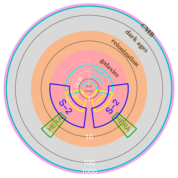
All neutral hydrogen in the universe below redshift of is in principle amenable to cm observations. This includes the large volumes at , the so-called “Dark Ages” before the first luminous objects were created; at , when these first objects formed and reionized the universe; and at , after reionization but difficult to fully map with large optical surveys. (See Figure 1 for a visual comparison of the volumes accessible to different kinds of observations and in different epochs of cosmic history.) In the Dark Ages and post-reionization era, the cm signal is a theoretically well-understood tracer of cosmic structure, and any science amenable to study through statistics of cosmic fields can be studied using this technique. However, the Dark Ages pose a formidable challenge (to say the least), for several reasons related to the low frequencies at which the associated observations must take place. Thus, we have identified the post-reionization era at as the most natural target for a dedicated next-generation cm instrument, although we will briefly discuss the high-redshift promise in Section 4.
In this white paper, we have not attempted to optimize the many design choices that must go into such an instrument. Rather, we have chosen a configuration that, while somewhat ambitious, is expected to comfortably fit within the cost profile of a typical DOE OHEP project, and performed a first round of forecasts for the scientific capabilities of this configuration. This exercise has allowed us to identify a trio of key science results that could be obtained by an instrument broadly in line with our chosen specifications, and also to explore a range of other applications of such an instrument.
The remainder of this introduction is as follows:
-
•
In Section 1.2, we summarize the three key science results, and a set of ancillary capabilities, associated with our fiducial instrument, which we have dubbed a “Stage ii” cm experiment.
-
•
In Section 1.3, we briefly introduce the basic mode of operation of radio telescopes in order to set the context.
-
•
In Section 1.4, we review the landscape of operational or planned post-reionization cm surveys, and place a Stage ii experiment in that context.
-
•
In Section 1.5, we introduce and discuss the practical challenges of implementing a Stage ii cm experiment.
-
•
Finally, in Section 1.6, we lay out a provisional roadmap for a three-stage cm program, building from “Stage i” (current experiments) through Stage ii and beyond.
-
•
In Section 1.7, we describe the synergies between optical surveys and cm experiments and unique advantages of each.
The main text of the paper is devoted to more detailed discussions of the various science cases (Section 2), the challenges and opportunities associated with Stage ii (Section 3), and a brief foray into observations 21-cm beyond redshift of (Section 4), with a discussion of current epoch of reionization experiments (Section 4.1) followed by a discussion of the exciting potential of the Dark Ages a probe of cosmology (Section 4.2). We conclude in Section 5.
1.2 Science capabilities of a large-scale cm experiment
The starting point for a Stage ii concept was the realization that the same instrument could help achieve three high-impact science objectives that are deeply connected to some of the biggest problems in fundamental physics. These are:
A1 Characterize the expansion history in the pre-acceleration era to the same precision as low-redshift measurements.
The precision of expansion history measurements in the low-redshift era using the BAO technique (see Section 2.3 for a technical description) is close to its theoretical limit due to the finite amount of large-scale information available per redshift. However, the measurement landscape deteriorates very fast for , and will not be satisfactory in this range for the foreseeable future. It is imperative to measure the expansion history to better than percent level all the way to , which allows measurement of the energy density in the dark energy component with the precision of 10% at those redshifts. In the pre-acceleration era, this is a very difficult measurement, because the total energy density and thus expansion history of the Universe is dominated by the matter density. Consequently, signatures of dark energy are expected to be small in a minimal CDM Universe. There is, however, strong theoretical motivation to explore this particular era, since theoretical explanations for the minimal CDM Universe generally suffer from extreme fine-tuning issues. Alternative explanations to CDM have generic signatures in the range, and percent-level expansion measurements within this range will impose stringent constraints on such theoretical models, which are otherwise unconstrained. Note that the Stage ii experiment will characterize the expansion history over the full redshift range starting at . However, the extragalactic sky at range will be mostly measured by a combination of Euclid and DESI, allowing only modest Stage ii improvements in this range. On the other hand, our measurements will represent an important cross-check of the results from the same volume using a fundamentally different tracer.A2 Characterize the growth rate of structure in the pre-acceleration era to the same precision as low-redshift measurements.
Similar to expansion history, the Stage ii experiment will also measure the growth of fluctuations across the redshift range from , with out determinations becoming particularly relevant in the high redshift regime . The method employed is similar to the redhift-space distortion measurements in galaxy cluster, but relies on the growth signatures in the weakly non-linear regime Castorina and White (2019); Modi et al. (2019a). In combination with expansion history over the same range of redshift, we would be able to potentially detect difference between the growth of structure and expansion rate, one of the smoking guns of modified gravity which would give a unique insight into the dark energy phenomenon.A3 Constrain or measure inflationary relics in the shape of features present in the primordial power spectrum.
Sufficiently sharp features in the primordial power spectrum survive mild non-linear evolution and biasing, and are predicted in various inflationary models. The amplitude, frequency and phase of the feature are all indicative of the mechanism that sourced the initial seeds of structure. If found, they would present a breakthrough discovery and unique opportunity in the attempt to understand the physics of the early Universe. It would be highly informative to constrain or detect the presence of oscillatory features with frequencies Mpc and amplitude smaller than relative to the inflationary power-law spectrum.A4 Constrain or measure the equilateral and orthogonal bispectrum of large-scale structure with unprecedented precision.
Primordial non-Gaussianities are generically predicted by non-minimal inflationary models of the early Universe. The size and shape of primordial non-Gaussianities would be indicative of the number of fields present as well as the strength of interactions and self-interactions of the field or multiple fields driving inflation. The huge amount of clean, large-scale statistics from the volume accessible to a high-redshift survey presents a unique opportunity to put unprecedented constraints on non-Gaussianities that are sensitive to the dynamics during inflation. Specifically, the three-point correlation function of Fourier modes of the density field (the so-called bispectrum) is amenable to measurement using high-redshift LSS surveys, and its amplitude in different configurations (corresponding to the three points forming squeezed, equilateral, or folded triangles) is directly connected to different inflationary models. Moreover, these types of non-Gaussianities (equilateral and orthogonal) cannot be constrained using bias constraints in the power spectrum and are therefore not amenable through cosmic variance cancellation techniques that are forecasted to put stringent constraints on squeezed non-Gaussianities. In other words, a high-redshift survey of the universe will most likely present the only viable opportunity to improve over CMB constraints.All three objectives described above could be achieved with a next-generation 21 cm experiment, which we designate a Stage ii experiment. Our fiducial configuration consists of a 50% fill factor hexagonally close-packed array of 32,000 m dishes, operating from 200 to MHz. This configuration is an ambitious but realizable expansion over the current generation cm experiments. Section 2.1 contains a technical arguments motivating this particular choice of fiducial experimental parameters. The precise configuration of the array and other experimental details are expected to evolve and be further developed depending on key science targets and experience obtained with predecessors of a Stage ii cm experiment. However, having an explicit experiment allows us to make concrete forecasts that set the context for further optimization.
The objectives outlined above directly follow from the ability of
cm emission to obtain a pristine picture of large-scale
structure with essentially no tracer shot-noise.
In the following, we list some of the other new capabilities that will be enabled by a Stage ii experiment:
B1 Add a new tracer at
By the time the Stage ii experiment becomes a reality, the volume of
the universe at redshift will be mapped by the current
and upcoming experiments using numerous tracers. These include
spectroscopic galaxies from DESI, photometric galaxies from LSST,
velocity measured by Hubble diagram residuals from type Ia supernovae,
gravitational wave siren sources, weak gravitational lensing from both
LSST and CMB, etc. Adding a new tracer will enable numerous new
studies, some of which we discuss in the Section
2.11, but the full breadth of potential new
science remains will likely be only fully understood as the field
evolves over the coming decade.
B2 Quadruple the observed volume at an increased fidelity.
The volume between and is approximately three times the
volume between and , and contains structures whose
clustering statistics are easier to predict than at lower redshifts
(see Figure 6). cm intensity mapping can probe
this volume with a very high effective number of sources, allowing for
straightforward extraction of cosmological information from these
measurements. While we have identified several well-motivated uses of the large
number of linear modes present in this volume as our main scientific
goals, other, yet to be discovered, statistical quantities describing
and constraining fundamental physics are also likely to improve
equally due to generic scaling of error on any derived statistical quantity.
B3 Measure information from scales and redshifts not directly present in the survey.
Couplings between different Fourier modes of the cosmic density field will allow us to reconstruct modes that are not directly present in the survey through their effects on the observed small-scale modes. In particular, the tidal effect of large-scale modes on the small-scale power will give access to the large-scale modes (which may otherwise be obscured by foregrounds in certain scenarios). Furthermore, gravitational lensing effects on small scales will provide information about lower-redshift structure. Three-dimensional cm observations will provide several source “screens” for lensing analyses; the signal to noise of a joint analysis of all such screens will exceed that for the next generation CMB lensing reconstruction in cross-correlation.
B4 Improve measurements of parameters that encode deviations from the minimal cosmological model, including neutrino mass, radiation content of the early universe, and curvature.
cm observations can, in
conjunction with other synergistic measurements, aid in constraining
these parameters. In particular, we should
achieve an independent detection of the neutrino masses and constrain the
radiation content to within a factor of a few of the guaranteed
correction due to electron-positron annihilation.
B5 Potentially directly detect the expansion of the Universe.
The
Universe expands at the Hubble rate and in principle this expansion
can be detected by observing sources drift in redshift over the time
of experiment. The advantage of radio observations is that the
clocks stable enough to drive the digitization circuits at the
required time stability are nearly off-the-shelf equipment.
B6 Explore the physics of fast radio bursts (FRBs).
This instrument will also likely detect millions of FRBs as we
discuss in Section 2.14. The physics of FRBs
is currently poorly understood, but in some models they could act as
standard candles or alternatively their dispersion measure in
conjunction with kinetic Sunyaev-Zeldovich effect measurements from
CMB could open another possible window into the expansion and growth
history of the universe.
B7 Explore modified gravity using pulsars.
The same
instrument that can be used for cosmology will also be able to
observe numerous pulsars and study general relativity through
precision changes in pulsar timings.
Using our fiducial Stage ii cm configuration, we will perform a detailed exploration of all possible science targets identified above in Section 2.
1.3 Observing the universe with a radio telescope
Radio telescopes observe the electromagnetic radiation at radio frequencies and for 21 cm this means at frequencies below 1.42GHz. A traditional single-dish radio telescope contains a focusing element, typically a parabola that focuses the incoming radiation onto a radio receiving element. Such parabola coherently adds all radio waves coming from a given direction. Such a telescope can observe a single pixel in the sky at once and the bigger the parabola, the higher is its resolution, with the sky response function scaling as roughly , where is the observing wavelength (redshifted from rest-frame ) and is the parabola size. Because radio wavelengths are very long (compared to typical optical wavelengths, for example), the size of the reflector needs to be very large to achieve a fine resolution.
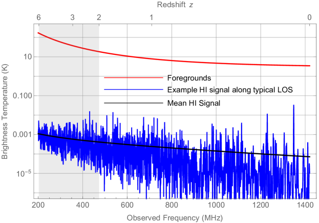
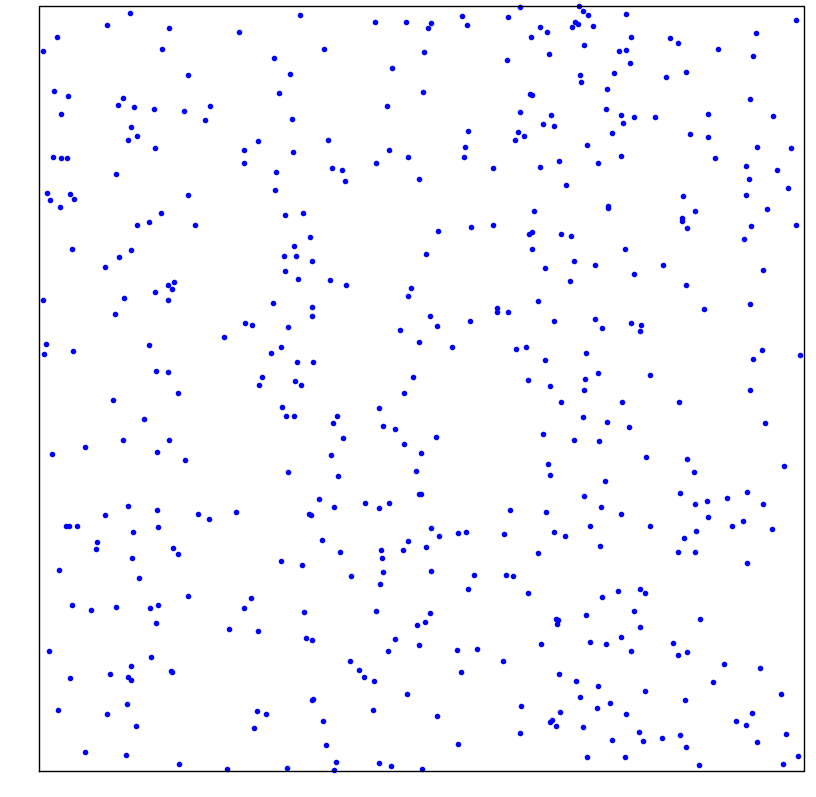
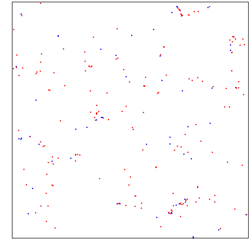
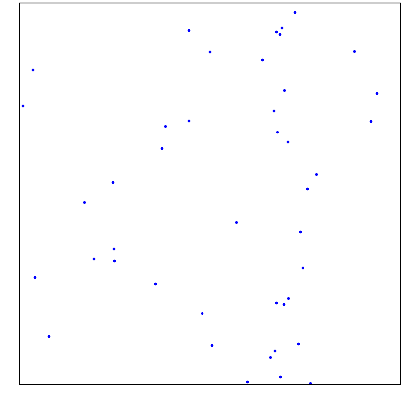
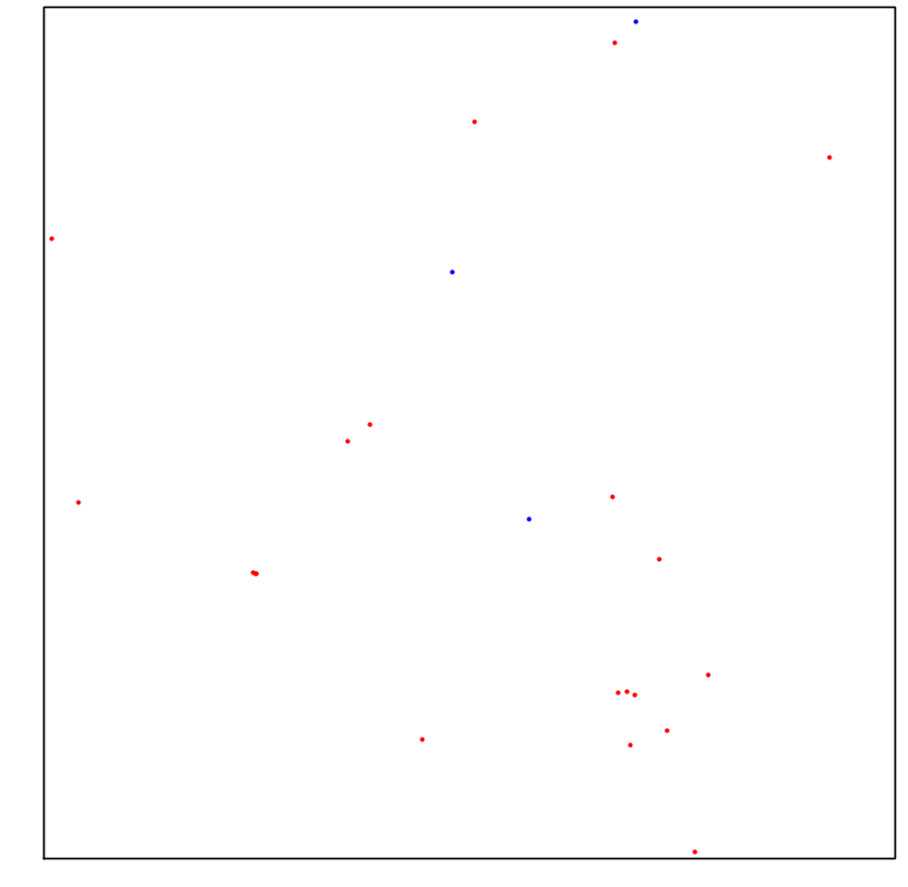
In Figure 2 we schematically show the signal observed by one such single-receiver pointed at a typical direction on the sky (and assuming it could observe signal from 200MHz to 1420Mhz). The signal would be dominated by the emission from our own galaxy – shown as the red line. This emission is very strong, but at the same time very smooth, which gives us a handle at subtracting it. The blue lines illustrates what the 21-cm signal would look like: at low redshift it would correspond to individual over-densities traced by small objects, while at high redshift the structure in the radial directions blurs into a continuous field.
It has long been recognized, that instead of combining the signals by optically adding them, one can add them electronically. This concept, known as aperture synthesis (for which the Nobel prize was awarded in 1974 to Martin Ryle) led to a class of instruments called radio interferometers. In such telescopes, the collecting area of a single dish is replaced with several individual smaller elements, that do not need to be, but are are often smaller dishes themselves. Signals form individual receivers are combined and allow one to synthesize an effective dish whose total collecting area is the sum of individual collecting areas and whose resolution matches that of a dish with the same size as the largest separation between individual elements. But the most important advantage is that multiple beams can be synthesized concurrently which can cover all of the primary field of view of individual elements. This can lead to an exponential increase in sensitivity compared to traditional single-element dishes.
In order to perform aperture synthesis, the signal from every pair of elements needs to be correlated and hence the difficulty increases as the square of the number of individual elements forming an interferometer. Therefore, traditional interferometers employed at most a few tens of elements. In the 21st century, however, digital technology allows the possibility of doing the signal combination digitally, leading to telescopes made of thousands of receiving elements. This progression in technology moved the complexity first from the problems of mechanical engineering in making large receiver dishes to that of building and replicating analogue electronics and finally to processing massive amounts of digital data. As we will see later, part of this white-paper continues this trend by arguing for digitization as soon as possible after the signal enters the system.
1.4 Post-reionization cm surveys: the state of the art
cm cosmology has only been made possible recently through developments in infrastructure (e.g. high-throughput computing and commodification of low noise radio-frequency technology) that allow for correlations at full bandwidth at the necessary scale. Tools and techniques have been developing rapidly, and the first steps towards extracting cosmological information from cm observations have already been demonstrated.
The first detection of the redshifted cm emission in the intensity mapping regime was achieved by Chang et al. in 2010 Chang et al. (2010). The measured 3D field, obtained from the Green Bank Telescope (GBT) 800 MHz receiver, spans the redshift range of to 1.12 and overlaps with 10,000 galaxies in the DEEP2 survey Davis et al. (2001) in spatial and redshift distributions. This enabled a cross-correlation measurement on 9 Mpc scales at a 4 significance level. This detection was the first verification that the cm intensity field at traces the distribution of optical galaxies, which are themselves known tracers of the underlying matter distribution. It presents an important proof of concept for the intensity mapping technique as a viable tool for studies of large-scale structure.
A continuing observing campaign to expand the GBT cm IM survey in both sensitivity and spatial coverage has yielded two subsequent publications: an updated cross-power spectrum at Masui et al. (2013) between cm and optical galaxies in the WiggleZ survey Drinkwater et al. (2010), and an upper limit on the cm auto-power spectrum Switzer et al. (2013). Combining the cross- and auto-power spectrum measurements yields a 3- measurement on the combination of the cosmic HI abundance and bias parameters, Switzer et al. (2013). Further analysis of 800 hours of GBT observations taken during 2010-2015 is currently ongoing.
No experiment has detected the cm power spectrum in auto-correlation. While this should be possible with non-dedicated experiments in terms of statistical significance, the instrumental challenges are currently too large. However, this situation should change with the advent of dedicated instruments.
There are currently five main experiments that are presently being built or are in the commissioning phase to measure LSS with the cm intensity mapping technique with dedicated instrumentation: CHIME in Canada, HIRAX in South Africa, Tianlai in China, OWFA in India, and BINGO, a UK/Brazil experiment. In addition, there are several smaller efforts dedicated to R&D, such as BMX at Brookhaven National Laboratory and PAON at Nançay in France. We list the main properties of these instruments in Table 1. These small-scale experiments will teach us about the viability of the intensity mapping technique, for example by providing testbeds for calibration, foreground removal, and RFI mitigation techniques.
Of the listed experiments, CHIME is currently the most advanced, and has recently upgraded from a prototype to the full instrument. It consists of 4 cylindrical radio antennas with no moving parts, observing the entire accessible sky which passes above it as the Earth rotates. It operates from 400-800 MHz, equivalent to mapping LSS between redshift to 2.5. We expect the first cosmology results from CHIME in the next 3 years, which should include foreground removal or mitigation techniques for intensity mapping measurements of LSS in cm emission. Note that CHIME has already shown promise related to one of its other science goals, having recently announced the first detection of a low-frequency fast radio burst Boyle (2018).
| Name | Optimized | Steerable | Type | Elements | Redshift | First light |
|---|---|---|---|---|---|---|
| Existing w data: | ||||||
| GBT | N | Y | Single Dish | 1 dual-pol on m dish | 0.8 | 2009 |
| Dedicated experiments: | ||||||
| CHIME | Y | N | Cylinder Interferometer | 1024 dual-pol over 4 cyl | 0.75 – 2.5 | 2017 |
| HIRAX | Y | limited | Dish Interferometer | 1024 dual-pol m dishes | 0.75 – 2 | 2020 |
| TianLai Dish | Y | Y | Dish Interferometer | 16 dual-pol m dishes | 0 – 1.5 | 2016 |
| TianLai Cylinder | Y | N | Cylinder Interferometer | 96 dual-pol over 3 cyl | 0 – 1.5 | 2016 |
| OWFA | N | Y | Cylinder Interferometer | 264 single-pol | 3.40.3 | 2019 |
| BINGO | Y | N | Single Dish | 60 dual-pol sharing 50 m dish | 0.12 – 0.45 | 2020 |
| Dedicated R&D: | ||||||
| BMX | Y | N | S. Dish + Interferometer | 4 dual-pol 4 m off-axis dishes | 0 – 0.3 | 2017 |
| NCLE | Y | N | Satellite | 35 m monopole ant. at Earth-Moon | 2018 | |
| PAON-4 | Y | limited | Dish Interferometer | 4 dual-pol 5 m dishes | 0 – 0.14 | 2015 |
| Non-dedicated: | ||||||
| MeerKAT | N | Y | Single-Dish | 64 dual-pol 13.5 m dishes | 0 – 1.4 | 2016 |
| SKA-MID | N | Y | Single-Dish | dual-pol 15 m dishes | 0 – 3 | 2023 |
| Proposed Here: | ||||||
| Stage ii | Y | limited | Dish Interferometer | 32,000 dual-pol 6 m dishes | 0.3 – 6 | 2030 |
Another experiment often mentioned in this context is the SKA444https://www.skatelescope.org/ (Square Kilometre Array). The SKA1-MID mid-frequency dish array is a formidable instrument, but is optimized for a variety of radio astronomy goals other than intensity mapping. In many aspects the comparison is similar to new generation of extremely sensitive optical telescopes that have mirror-sizes exceeding 30m, but are nevertheless not competitive for survey-science optical cosmology due their small field of view and focus on diffraction-limited imaging of individual objects. For intensity mapping, SKA1-MID suffers from a similar mismatch in scales to which it is sensitive compared to the proposed Stage ii experiment. While it will typically act as an interferometer with several hundred large dish elements, the baseline distribution best matches the scales relevant to imaging of individual objects rather than intensity mapping of large-scale structure. As a workaround, the SKA1-MID array will instead be used as a collection of single dishes for intensity mapping, perhaps using interferometry only as a calibration tool. This will have relatively poor angular resolution at however, leaving it sensitive mostly to only the radial BAO feature (Villaescusa-Navarro et al., 2017). Additionally, individual elements of SKA1-MID are highly capable fully-steerable dishes that can operate up to 14 GHz. Dedicated designs for cm intensity mapping survey science typically use transiting arrays instead, since one wants to maximize the sky coverage rather than point at objects of interest, and reduce mechanical costs; cm intensity mapping also requires considerably lower maximum frequencies and corresponding dish-surface accuracy requirements (i.e. 500 MHz for our Stage ii experiment and never higher than the frequency of neutral hydrogen at 1420 MHz). It is clear that the SKA1-MID instrument has been optimized for different science goals and has therefore embarked on a different set of trade-offs to an optimal cm experiment. As such, it will not be directly competitive with dedicated instruments for many of the science cases discussed in this document, and thus does not present an obstacle to DOE for entry into this field. The same is true for the SKA1-LOW instrument, which partially overlaps in frequency coverage with our proposed Stage ii experiment (i.e. at the high redshift end of our band), but has a greater focus on Cosmic Dawn and Epoch of Reionization science, and will not be competitive with Stage ii for BAO measurements for example (see Bull (2016) for cosmological forecasts for SKA1-MID and SKA1-LOW surveys). Nevertheless, as the largest and most complex radio astronomical facility to be constructed in advance of Stage ii, we expect SKA to offer a number of valuable lessons in terms of calibration and data analysis techniques, computing infrastructure, and data management.
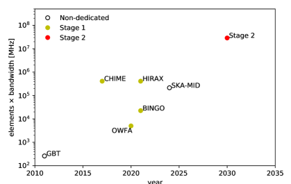
In Figure 3, we plot the same information as Table 1, but compressed into in a figure of merit analogous to optical etendue measure:
| (1) |
This equation is motivated by the expression for the system temperature contribution to noise (see Eq. 20 in Appendix D) and it is necessarily a very crude simplification. Most importantly, it does not take into account the surface area of reflector material and would naturally drive you towards a field of dipole antennas at fixed cost. While this might be the right answer in the absence of systematic effects, the current consensus is that some directionality of individual elements is desirable. Moreover, a compact interferometric array with the same figure of merit will in general perform better than a traditional radio array with the same figure of merit for the science discussed in this paper. Finally, observing at different central frequency affects the result in a non-trivial way: the sky noise is lower at higher frequencies, but the volume per unit bandwidth is larger at lower frequencies and the Universe is more linear at higher redshifts.
 |
 |
 |
 |
 |
 |
 |
 |
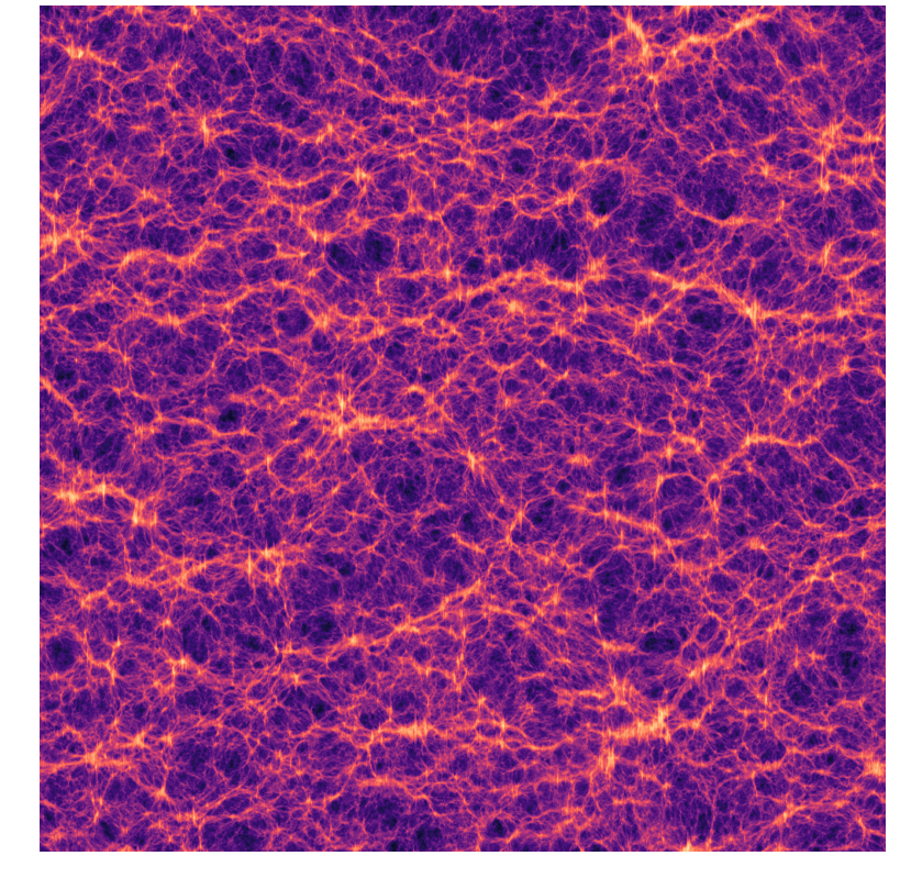
Nevertheless, with these caveats in mind, the figure of merit in Eq. (1) is a rough proxy of instrument capability and Figure 3 shows the improvement with time of the current and proposed experiments. To visually demonstrate the capability of a Stage ii experiment, we refer reader to Figures 4 and 5. These figures display how the proposed instrument would faithfully measure the structures in the Universe up to very high redshifts at the large scales relevant to cosmological analysis.
We again iterate that this section was focused on the post-reionization experiments. There is a vibrant community of epoch of reionization cm experiments and ideas for even higher redshift. These share many of the technical issues with the Stage ii experiment even though the science is considerably different and are discussed in Section 4.
1.5 Practical challenges
There are several known issues for achieving cm cosmology goals compared to traditional galaxy surveys. These call for a coherent development plan that will allow this technique to reach its full potential. We stress that the challenges are in the instrument and not fundamental to the signal: with sufficient care, we can build a calibrated system that will be dominated by statistical rather than systematic errors. These complications and our suggested mitigation for a successful survey are:
-
•
Loss of small- modes. The foreground radiation is orders of magnitude brighter than the signal, but spectrally smooth (see Figure 2 for a schematic illustration). Thus, the signal can be isolated but only for modes whose frequency along the line of sight () is sufficiently large. As a consequence, the low- modes are lost and this precludes direct cross-correlation with tomographic tracers such as weak lensing. However, as we discuss, these modes can be reconstructed from their coupling to the measurable small-scale modes, with non-trivial precision for a sufficiently aggressive system.
-
•
The foreground wedge. Interferometers are naturally chromatic instruments, since their fringe patterns—and therefore the cosmological lengthscales that they probe—are dependent on frequency. This can cause extra spectral features to be imprinted on the (in principle) spectrally smooth foregrounds. For a power spectrum measurement, this results in a set of Fourier modes on the - plane (“the foreground wedge”) that are heavily contaminated by foregrounds. This problem becomes more important at higher redshift and is acute for epoch of reionization experiments. We note that there is nothing fundamental about this problem: the mathematics behind the wedge are well-understood Parsons et al. (2012); Liu et al. (2014a), and thus an appropriate analysis pipeline applied to a well-calibrated system with sufficient baseline coverage can in principle perfectly separate the foregrounds from the signal even inside the wedge Liu et al. (2014b); Ghosh et al. (2018). The problem is therefore primarily a technical challenge rather than a fundamental limitation. We discuss our modeling of, and assumptions about, the foreground wedge in Appendix C.
-
•
The mean signal is not measured. Because the mean signal is not measured, the redshift-space distortions in the linear regime are related to the growth parameter via an unknown constant. Cross-correlations with optical surveys Chen et al. (2019) and modeling the mildly-non linear regime of structure formationcCastorina and White (2019) are effective ways to break this degeneracy.
These issues need to be studied in detail, both in theoretical terms and through a vigorous experimental program. We argue that major US agencies should support this research program in order to allow truly competitive experiments to become reality in the coming decades.
1.6 Roadmap
This white paper argues for a long-term development of the cm cosmology program in the USA, led by the Department of Energy but working in conjuction with other agencies where shared science warrants cooperation. In particular, a similar model to that of LSST is envisioned, in which DOE takes up particular aspects of the development which are well matched to its expertise and a collaborating agency takes over some of the other aspects that might not be an optimal fit for the DOE. To this end, we argue for a staged approach that includes three nominal steps leading to a Dark Ages experiment, as outlined in Table 2.
![[Uncaptioned image]](/html/1810.09572/assets/x4.png)
-
•
Our first step in the roadmap is an era of vigorous research and development, probably in conjuction with a small-scale test-bed experiment. During this stage, the following should be accomplished:
-
–
Refine the scientific reach of a Stage ii experiment. In Chapter 2 we start this process by describing some of the exciting science that is achievable using a straw man design. The design of the instrument should be driven by science and not the other way round, but in practice one needs to start with a given design to see the ballpark science achivable and then iterate until a convincing science-driven experiment design emerges. Our Chapter 2 is the first step in this direction.
-
–
Advocate for support from major scientific commissions. In particular, the 2020s Astronomy and Astrophysics Decadal Survey and the next P5 report will need to strongly endorse this technique to keep it a viable option.
-
–
Resolve technical challenges. There are numerous technical challenges, particularly in terms of calibration and data analysis. We suggest a two-pronged approach: first to benefit from the experience of current-generation experiments in mitigating these challenges, and second to support instrumentation development and theoretical progress using a combination of computer simulations, lab experiments, and small, dedicated pathfinder instruments. We describe this program in greater detail in Section 3.
-
–
Optimize a Stage ii instrument configuration. Parameters like redshift range, number of elements and their optical designs, calibration schemes, etc. can crucially affect scientific outcome. We will refine and optimize the array parameters to both minimize the systematic effects and maximize possible science.
-
–
Maintain flexibility in approach. New exciting scientific developments obtained with optical surveys will be considered when designing the cm array proposed here. For example, a sign of early dark energy might motivate a shift towards higher redshift, while evidence for a non–cosmological-constant equation of state parameter, , might favor lower redshift. Moreover, if fast radio bursts turn out to have useful cosmological applications, they might also affect various design choices. The most important point is that sufficient resources must be available at this stage to develop the technique and maximize its promise.
-
–
-
•
The next step is a post DESI/LSST experiment, which we call a Stage ii experiment in this document, becoming reality in the later part of the next decade. To reach interesting cosmological constraints, the experiment will have to be an order of magnitude larger than current experiments. In this document we consider a particular fiducial Stage ii experiment operating at redshifts , whose parameters we discuss in Section 2.1. The main scientific output of this survey will come from surveying the high-redshift universe, but because the majority of the cost is in the infrastructure and metal, we have not sacrificed the low-redshift component, which will offer ample cross-correlation opportunities and moderate increase in total signal-to-noise. However, this particular aspect of the design, as any other, remains on the table to be changed and optimized as we learn more about the most compelling scientific targets.
-
•
If successful, we expect this could be followed by a Dark Ages experiment. This is the most vaguely defined and forecasted instrument, and will require significant improvements and R&D, pushing its timeframe to two or three decades from now. To motivate an experiment probing the high redshift cm signal, we discuss some of the unique science opportunities in Section 4.2. The most important aspect is that there exists a long-term scientific opportunity which could be built on top of the Stage ii experiment.
1.7 Synergies with optical surveys
Optical galaxy surveys are now a mature observational tool, having gone from pioneering surveys of a few thousand galaxies, through definitive detections of cosmological clustering signals like baryon acoustic oscillations, to now routinely producing precision cosmological constraints. This successive, multi-generational development path continues, as next-generation experiments like DESI are poised to improve over current experiments by an order of magnitude in depth, and by pushing to significantly higher redshifts.
The cm intensity mapping technique is much earlier along its
development track, and must yet pass through a series of milestones
before it can be considered truly competitive with optical surveys. We
can already discern some of the main synergies with the optical
surveys:
3D information.
Optical galaxy surveys fall into two categories: either they survey a huge
sample of galaxies at low redshift resolution (photometric) or survey a subset
of selected galaxies at high redshift resolution (spectroscopic). However, in
both cases we have additional information about galaxies: from photometric
surveys the actual image of the galaxy can be used to infer not just galactic
morphology, but also gravitational lensing and the detailed optical spectra can
be used to infer physical properties of the galaxy, such as star formation.
cm surveys on the other hand provide an avenue that identifies galaxies
and at the same time recovers their redshifts (in an aggregate sense) allowing an
efficient mapping of the full 3D structure in our Universe. This inevitably
loses some information that can be present in the full optical survey, but
offers a complementary path towards a cost-effective survey at high redshift.
Shot noise vs sample selection.
Any point tracer of
large-scale structure suffers from the fact that we are sampling a
continuous field using a finite number of objects. This Poisson
component, also known as shot noise, acts as a source of noise in any
statistics derived from the large-scale structure observable. To
reduce shot noise, one needs to take spectra of more objects, but most
often there simply are not enough objects up to a given flux, limiting
the ability to mitigate shot noise. In cm observations, we are
measuring integrated intensity from all objects, even the very small
and faint ones, and so the shot noise is lower by several orders of
magnitude. In fact, all Stage i experiments will be limited by
continuous sources of noise (sky noise and thermal amplifier noise)
and only Stage ii will start to be sensitive to the underlying shot
noise. On the other hand, optical surveys allow one to slice the
galaxy sample into individual sub-samples that can be selected to have
certain properties. Together, both techniques offer complementary
views of the
same underlying structure.
Scaling with redshift.
Optical measurements excel at lower
redshifts, but they become increasingly difficult as the redshift range of
surveys is pushed towards the more distant universe. First, observations must be
performed in the infrared, where they suffer from brighter sky that has many
more sky-lines which are also more variable than in the optical. Second, the
infra-red detectors are more expensive and less efficient than optical
charge-coupled devices (CCDs). Third, the objects themselves are fewer in
number and fainter, since we are observing a younger universe. In radio, the
primary limitation is from foreground emission; however, the same foreground
removal techniques vetted by previous generations of cm experiments can be
applied because the foregrounds do not fundamentally change across the redshift
range of interest. In addition, at higher redshifts, the same bandwidth covers
more cosmic volume and requirements on things like reflector surface accuracy
become less demanding. In short, for the universe, optical surveys offer
many advantages and offer an excellent tool for studying the universe down to the
smallest scales, but radio techniques scale better towards higher redshift.
2 Science case for a post-reionization cm experiment
This section focuses on preliminary science forecasts for a Stage ii cm experiment to demonstrate the potential science reach of such an instrument. A Stage ii experiment refers to an experiment that will build upon the current, non-US, Stage i, pathfinder telescopes such as CHIME and HIRAX. We focus on redshifts after reionization () that will be mostly unexplored by optical surveys. We design an array to probe these redshifts, based on what would be possible with current technology at a price-point that is consistent with a medium-size high-energy-physics experiment. In this Chapter we envision a realistic experiment that is “shovel-ready”, assuming the technical challenges discussed in the next chapter are feasible and Stage i experiments do not uncover any unexpected significant issues.
We will describe the science potential that our proposed design could achieve, briefly in Section 2.1 and then in more detail in the following subsections. We conclude with a discussion of other relevant science. In this version of the document, we assume PUMA parameters Bandura et al. (2019) as a concrete realization of the Stage ii concept, because its design has been optimized in outline for the science goals at hand. In later stages of the planning process the science goals and instrument parameters will be refined further with a proper flowdown study, likely motivating various modifications or improvements to the design choices we present here.
2.1 Science drivers and the straw man experiment
As outlined in the introduction, there are three main science drivers for the proposed experiments: measurement of the properties of dark energy in the preacceleration era (goal A1), constraints or detection of inflationary relics in the shapes of features present in the primordial power spectrum (goal A2) and constraints or detection of non-Gaussian correlations in the primordial fluctuations (goal A3).
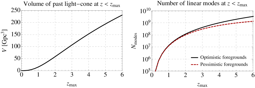
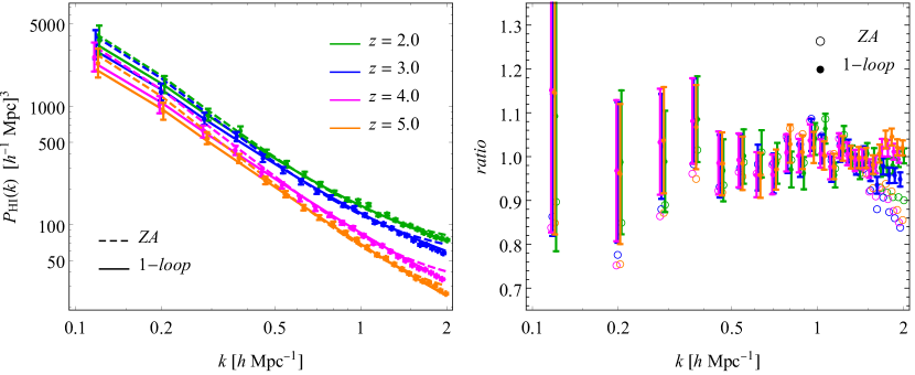
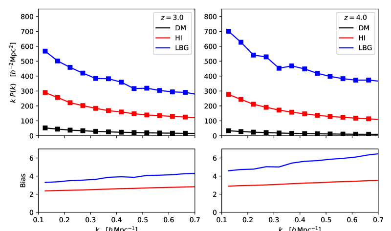
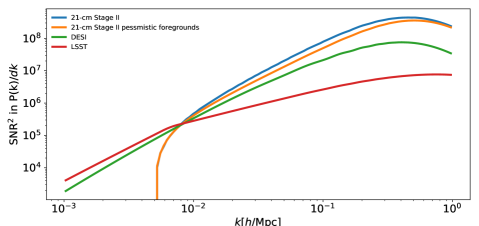
Goals A2 and A3 are best served by an experiment that has access to a large number of linear or quasi-linear modes. Given a sufficient density of tracers, the total number of modes scales as , where is the survey volume and is the maximum wavenumber amenable to theoretical predictions. Going to higher redshift helps both cases. First, there is more volume per unit redshift at higher redshifts: as indicated in the left panel of Figure 6, the total volume available over is roughly triple the volume at . The effect is even more pronounced if one considers the amount of cosmic volume per unit bandwidth of the radio signal. Second, at a given comoving wavenumber , the field is more linear at higher redshift, leading to an increase of . This translates into a large increase in the number of usable linear modes at higher redshift, as shown in the right panel of Figure 6 (see App. A for the details of our definition of “linear modes.”). Figure 7 confirms that even low order perturbation theory calculations can accurately describe the results of hydrodynamical simulations out to a sufficiently high wavenumber. Though it is not shown in Figure 7, the cross-correlation between the observed and initial fields also remains higher to smaller scales for the cm field. Finally, the bias of the cm field is less scale dependent, and easier to model, than a coeval population of galaxies because the neutral hydrogen traces lower mass halos (Figure 8). This effect becomes particularly pronounced at the highest redshifts.
By a fortunate coincidence, all three science drivers naturally lead to a high-redshift experiment. The upper limit is set by the requirement that the universe has reionized and thus astrophysics does not limit our modeling, which requires or the low frequency edge of 200MHz. The lower limit is set by what we think are practical considerations in terms of the maximum fraction bandwidth that we believe is credibly obtainable. Based on Vanderlinde (2019), we set the upper frequency limit to MHz, resulting in a lower redshift limit to . This gives the total bandwidth of 5.5, somewhat lower than three octaves.
In Bandura et al. (2019), we have identified a 32000 array of 6-m dishes operating at 200 – 1100 MHz as a straw man configuration that would achieve the three main scientific goals specified above. The Science Traceability Matrix developed for PUMA for the same goals as discussed here, calls for hexagonally closed packed array with 50% fill factor. We adopt the same configuration in this revision of the roadmap document, unless stated otherwise. Such experiment is 30 times larger than the partly funded HIRAX experiment, currently under construction in South Africa. The total collecting area of such experiment would be around 0.9 square kilometers. While this is more than SKA, we stress that the low frequencies and in particular the non-actuating nature of the transit arrays makes such a design orders of magnitude cheaper. We assumed a 5-year on-sky integration, requiring a somewhat longer total duration of experiment, but note that compared to optical experiments the achieved observing efficiency can be considerably larger since radio telescopes can often observe during the day and through cloudy weather.
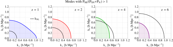
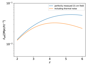
In addition to the main science goals, such experiment would enable a wide range of other science, both in the field of cosmology and fundamental physics as well as in related astrophysical sciences that could be of interest to a broad community. One can obtain intuition for the range of available science by asking which modes of the 21 cm temperature field will have signal higher than the sum of thermal and shot noise. We show this at a few representative redshifts in Fig. 9, finding that can be achieved for all linear modes at and all modes with at . In the rest of this chapter, we study a subset of the most interesting science that would come from this experiment, with a focus on the cosmological arena.
In our forecasting we assume the existence of the DESI and LSST experiments. When relevant we also discuss and compare with the CMB-S4 survey, but we note that its final design is less certain than that of DESI and LSST. In some sections, we impose additional 2% or 5% priors on cosmic neutral hydrogen abundance, as motivated by Castorina and Villaescusa-Navarro (2017) or achievable using cross-correlation with other tracers. The results presented in this chapter were derived using several forecast codes. The common assumptions used to forecast main results can be found in Appendices B, C and D, but even when slightly different assumptions are used the results are typically consistent to around 20% in accuracy over the relevant scales. We regard this as sufficient at this early stage. Throughout this chapter we will present forecasts for foreground optimistic and foreground pessimistic case that are likely to bracket the true value of what level of foreground cleaning is realistically achievable for the Stage ii experiment.
2.2 Early dark energy and modified gravity
A concerted, community-wide effort to explain the origin of cosmic acceleration has uncovered a vast zoo of dark energy and modified gravity models. These can be broadly classified according to how they modify GR or replace the cosmological constant, – for example, by adding new scalar, vector or tensor fields; adding extra spatial dimensions; introducing higher-derivative or non-local operators in the action; or introducing exotic mechanisms for mediating gravitational interactions Jain and Khoury (2010); Clifton et al. (2012); Weinberg et al. (2013); Joyce et al. (2015, 2016); Amendola et al. (2018). A summary of some possible new gravitational phenomena that can result from these modifications is included in Table 3.
![[Uncaptioned image]](/html/1810.09572/assets/x9.png)
A systematic study of these models suggests a number of new gravitational phenomena that can arise if there are any deviations from the standard cosmological model. These include the possibility of a time-varying equation of state for the component that sources the cosmic acceleration; time- and scale-dependent variations in the gravitational constant (leading to modifications to the growth rate of large-scale structure and gravitational lensing (Amendola et al., 2013a; Jain et al., 2013; Amendola et al., 2013b; Baker et al., 2014a; Leonard et al., 2015)); and ‘screening’ effects, where the strength of gravity becomes dependent on the local environment (Khoury and Weltman, 2004; Hinterbichler and Khoury, 2010; Brax et al., 2012; Jain et al., 2013; Koyama, 2016). It is also the case that current constraints on possible deviations from GR are quite weak on cosmological scales, compared to the extremely precise measurements that have been obtained on Solar System and binary pulsar scales (Baker et al., 2015; Berti et al., 2015). The application of GR to cosmology therefore represents an extrapolation of the theory over many orders of magnitude in scale from where is has been well tested. Constraints on GR on cosmological scales are therefore a natural programmatic goal for cosmology.
Observational constraints on possible deviations from GR+ are only now becoming sufficiently accurate to constrain a wide variety of these scenarios. Recent theoretical work has significantly simplified the task of testing dark energy and modified gravity theories, by collecting many possibilities into a handful of broad classes, such as the Horndeski class of scalar field theories, which can then be studied in a general sense, instead of on an individual ‘model-by-model’ basis Gubitosi et al. (2013); Bloomfield et al. (2013); Bellini and Sawicki (2014). Although measurement of the speed of propagation of gravitational waves based on the gravitational wave event GW170817 and its electromagnetic counter-part GRB170817A Abbott et al. (2017) has tightly constrained a large number of possible modified gravity theories Lombriser and Taylor (2016); Creminelli and Vernizzi (2017); Sakstein and Jain (2017); Ezquiaga and Zumalacárregui (2017); Baker et al. (2017); Amendola et al. (2018) (although see Ref. de Rham and Melville (2018) for a critique that may mitigate this conclusion), large parts of parameter space remain unconstrained.
One can make predictions for observables within the context of these general classes, to see where the possibility of detecting a (potentially quite small) deviation from the standard cosmological model might be maximized. This exercise has so far been performed for a handful of theory classes and observables. In Raveri et al. (2017), for example, generic predictions were obtained for the behavior of the equation of state of dark energy , within the full Horndeski class. Interestingly, many of these theories predict a ‘tracking’ type behavior, where scales along with the energy density of the dominant fluid component at any given time. This leads to the expectation that at low redshift, , where dark energy begins to dominate, but at higher redshift, deep within the matter dominated regime. This behavior is caused by couplings between the scalar field and the matter sector that generically arise in many branches of the Horndeski theories (although tracking can also be realized in models without such couplings, e.g. freezing quintessence models (Linder, 2006a)). The fact that this behavior is a reasonably generic prediction of a large and important class of models (most scalar field dark energy theories are included within the Horndeski class) highlights the need for precision observations in the intermediate redshift regime, . If the equation of state can be reconstructed at these redshifts, possible tracking behaviors can be either definitively detected or thoroughly ruled out. Without such direct observations however, it will be difficult to tell whether a transition is occurring, or whether a possible disconnect between observations at low and high redshifts is due to some other factor (e.g. systematic effects). In Section 2.3 we discuss how the Stage ii experiment will measure the expansion history at sufficiently high redshifts to constrain these models.
It is similarly important to test the growth rate of large scale structure over a range of redshifts, to ensure that possible deviations from GR on large scales have not been missed or absorbed into constraints on other parameters at late times (di Porto and Amendola, 2008; Simpson and Peacock, 2010; Baker et al., 2014b; Perenon et al., 2015). As with the equation of state, the range is currently lacking in direct observational probes of the growth rate. In Section 2.5 we will discuss ability of Stage ii experiment to measure the growth rate at high redshift.
Finally, we observe that 21 cm is uniquely sensitive to very small halos, where galaxies are usually too faint to be observed directly. Some of the modified gravity theories that pass all current observational tests predict that the abundance of those light halos could be a sensitive probe of gravity modifications, rendering Stage ii a unique probe Leo et al. (2019).
2.3 Measurements of the expansion history
Baryonic Acoustic Oscillations have been a staple of survey science for the past decade. They allow measurements of the expansion history of the universe, whose relative calibration is naturally below percent level and whose absolute calibration depends only on the well understood plasma physics in the early universe.
In the early Universe, before hydrogen recombination, electrons, baryons and photons formed a tightly coupled plasma with a short mean-free path. Perturbations in this plasma, seeded at much earlier times by inflation, propagated as acoustic waves until the photons decouple from the plasma at recombination. The compressions and rarefactions in the plasma leave an imprint on the distribution of matter in the Universe at a characteristic scale of : the speed of sound in the primordial plasma times the age of the Universe at decoupling. This scale is most commonly measured from the peak in the correlation function or, equivalently, the series of oscillations in the power spectrum known as baryon acoustic oscillations (BAOs; see Refs. Weinberg et al. (2013); Percival (2017); Tanabashi et al. (2018) for recent reviews).
These correlations have been successfully detected using galaxies, quasars and the Lyman- forest Alam et al. (2017); du Mas des Bourboux et al. (2017); Slosar et al. (2013); Ata et al. (2018); Kazin et al. (2014). In fact, due to the large scales involved and the differential nature of the measurement (one or more peaks on top of a smooth background signal), BAOs are among the most robust measurements in cosmology. Because the physics of early universe is well known, and highly constrained by CMB observations, the BAO method provides a well-calibrated standard ruler Aghanim et al. (2018a). With such a ruler BAOs can robustly measure the comoving angular diameter distance, , using transverse modes and the expansion rate, , using radial modes; both as a function of redshift. For this reason current and future spectroscopic surveys (e.g. Alam et al. (2017); Aghamousa et al. (2016); Laureijs et al. (2011) or Table 1) have BAO as a major science driver. A measurement of BAOs at , complementary to the next generation of experiments, is one of the scientific opportunities in our proposed Stage ii experiment.
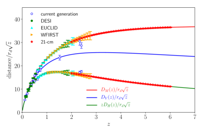
In Figure 10 we estimate constraints on the distance scale from a Stage ii experiment. The forecasting was done using the standard approach of Ref. Seo and Eisenstein (2003), adapted for cm measurements. In particular, at each redshift bin, we add the shot-noise and thermal noise contribution at wavenumber Mpc to power spectrum, and convert these back to an effective number density of sources. The results are largely independent of choice of fiducial at which we do this conversion. Figure 10 shows that current and next generation optical/IR experiments lose constraining power at , while we forecast a Stage ii cm experiment can map the expansion history with high precision all the way to up to the end of epoch of reionization ().
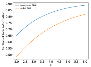
The high precision achievable with a Stage ii experiment is due in part to the very high number density of cm sources, which provide sample-variance limited measurements of the relevant scales. The cm signal is dominated by numerous, small galaxies with number densities greater than . This can be compared to typical values for galaxy surveys which are around or less. We plot these numbers in the left panel of Figure 11. The effect of the thermal noise of the system (which is not present in optical galaxy surveys) does lead to a decrease in the effective number density of sources but for our Stage ii survey this is a modest change. Provided foregrounds can be controlled, we are close to saturating the information content in BAO that can be achieved over half the sky – no future BAO experiment could do significantly better as illustrated in the right panel of 11.
 |
 |
2.4 Cosmic inventory in the pre-acceleration era
The measurements of the cosmic expansion history and distance-redshift relation described above constrain the abundance and time evolution of the various components of the cosmic fluid. Radial BAO directly probe the expansion history, , while the angular BAO are related to the angular diameter distance,
| (2) |
Within GR, both are related to the evolution of the sum of the energy densities of components in the Universe
| (3) |
Since the scaling of the energy density with time is known for matter, radiation, curvature, and neutrinos, the redshift dependence of can be used to infer the time dependence of the dark energy density. Assuming basic thermodynamics, this is in turn determined from the dark energy equation of state, . As discussed in previous sections, is an extremely interesting quantity for studying dark energy models, and is being increasingly well constrained at relatively low redshifts, , where dark energy is a large fraction of the total cosmic energy density. In Section 2.2, we discussed a number of theoretical reasons why the equation of state might be near at low redshift but transition to at higher redshift, making it difficult to definitively distinguish dynamical dark energy from a Cosmological Constant using only low measurements. Indeed, some models only show large deviations from at , where dark energy is already a subdominant component of the cosmic energy density Doran and Robbers (2006); Karwal and Kamionkowski (2016); Raveri et al. (2017). This makes these ‘early’ dark energy scenarios relatively difficult to probe, as even quite large changes in equation of state only have a small effect on the total cosmic energy density Bean et al. (2001); Xia and Viel (2009); Calabrese et al. (2011); Pettorino et al. (2013); Aghanim et al. (2018a). BAO measurements from a Stage ii cm experiment will make it possible to measure the energy density with sufficient precision to put constraints on early dark energy scenarios however, allowing us to constrain this class of (scalar field) dark energy models.
To illustrate this, Figure 12 shows current and forecast constraints on the energy density of dark energy as a function of redshift. We compare two models that allow early dark energy behaviors, while also admitting a fiducial flat CDM case – ‘mocker’ models (Linder, 2006a, b), which are a particular class of quintessence models with a smooth transition to a matter-like equation of state at high redshift; and ‘tracker’ models, which are phenomenological models with a smooth step-like transition in the equation of state, motivated by the Horndeski model priors discussed in Section 2.2. The mocker models are minimally-coupled, and so are constrained to not cross the phantom divide (i.e. go from to ), while the tracker models are not subject to this restriction.
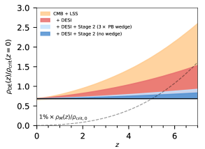
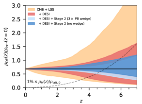
In both cases, it can be seen that current data (CMB plus BAO at ) constrain any early dark energy component to be less than about 3% of the cosmic energy density at , with significant growth (or decay) in the energy density allowed. Adding the DESI constraints at would improve the upper limit to around 1% at , while still allowing considerable deviations from a cosmological constant – e.g. by a factor of 2 in energy density at for the Mocker models. Adding a Stage ii cm experiment, covering , improves the constraints by at least another factor of two, depending on the model, even in the foreground pessimistic case. This is a significant improvement considering that the dark energy density is strongly subdominant at these high redshifts.
2.5 Growth-rate measurement in the pre-acceleration era
Redshift-space distortions are an anisotropy of the power spectrum along the line of sight caused by the peculiar velocities of sources that add to the cosmic redshift. Since these velocities are sourced by the same fluctuations in the universe, the result is a particular distortion of the power spectrum. To lowest order, these distortions multiply the standard power spectrum by , where is the large-scale bias, is the cosine of the angle to the line of sight and is the logarithmic derivative of the growth factor. Given that the shape of power spectrum is known to a good degree, redshift-space distortions in traditional radio surveys measure , where is the linear-theory value of the rms fractional fluctuations in density averaged spheres of Mpc radius at . The CDM model, constrained by current CMB observations Akrami et al. (2018); Aghanim et al. (2018a), predicts both and at to better than 0.5% (or about 1.1% if we allow neutrino masses to vary). This provides a firm prediction which can be tested using precise observations at high .
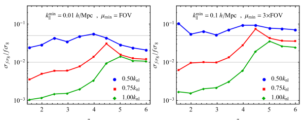
In cm, the mean signal is unknown, so in effect linear redshift-space distortions instead measure the product , with being a nuisance parameter. However, there are three main ways to go around this limitation. The first is to use the method of Ref. Obuljen et al. (2018), namely measure the bias and brightness temperature from complementary data such as the Lyman- forest, where the sources relevant for cm emission appear as individually detected hydrogen systems (for a summary of our current understanding of the uncertainties in neutral hydrogen abundance, see refs. Crighton et al. (2015); Padmanabhan et al. (2015); Rhee et al. (2018)). Assuming the foreground contamination can be brought under control, the resulting constraints are dominated by this prior if it is weaker than Obuljen et al. (2019). Alternatively, it is possible to cross-correlate with other tracers at the same redshift as we discuss in Section 2.11 and Figure 19. Finally, one can use beyond-linear effects to break the degeneracy between and Castorina and White (2019); Modi et al. (2019a). All methods allow redshift-space distortions to be measured with the precision of a few percent. This also happens to be close to the current level of theoretical uncertainty in the modeling of redshift-space distortions. Figure 13 shows the RSD constraints between achievable by Stage ii cm for different foreground removal assumptions, in the left panel an optimistic case and in the right panel a more pessimistic one. Different colors show the smallest scales, largest wave number , included in the forecast in units of the non linear scale . We consider somewhere between the red and green line a realistic scenario, for which Stage ii cm will be able to measure RSD at a few % precision even in the most pessimistic cases.
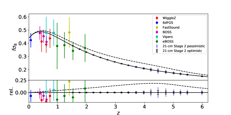
We replot the same data in Figure 14 for the red curve together with a selection of current constraints for comparison Blake et al. (2012); Beutler et al. (2012); Okumura et al. (2016); Beutler et al. (2017); de la Torre et al. (2017); Zhao et al. (2019). The theoretical models are the fiducial CDM model (plotted as a solid black line) and a moderately tuned modified gravity model (plotted as a dashed black line) chosen so that the expansion is unaffected at and the effects are small at low redshift. In particular, we use the Horndeski formalism of Ref. Bellini and Sawicki (2014), with the expansion history fixed to mimic CDM, (motivated by LIGO results) and other parameters proportional to with and . The theoretical models are generated using the hi_class package (Zumalacárregui et al., 2017; Blas et al., 2011). It is clear from the plot that the Stage ii will be extremely powerful in telling departures from CDM growth of fluctuations over significant portions of the evolution of the universe.
2.6 Features in the primordial power spectrum
The baryon acoustic oscillations are well-understood features in the matter power spectrum that are introduced during the evolution of the universe. In addition, there might be other oscillatory features of various origins in the power spectrum that we can search for with a Stage ii experiment. In general, the matter power spectrum at a wavenumber and redshift is in linear theory given by
| (4) |
where is the transfer function and is the dimensionful primordial power spectrum. Assuming standard slow-roll inflation, the power spectrum of curvature perturbations is well approximated by a power law ( with Akrami et al. (2018); Aghanim et al. (2018a)). However, numerous mechanisms could have imprinted oscillations around this power law in the primordial spectrum (see e.g. Chluba et al. (2015); Slosar et al. (2019a) for recent reviews), while exotic physics in the dark sector can add additional features to the transfer function (see e.g. Cyr-Racine et al. (2014)).
Detecting a deviation from a featureless power spectrum of primordial fluctuations would provide unique insights into the physics of the primordial universe. These features can provide evidence for particular inflationary scenarios, or identify the existence of new particles and forces during inflation or in the thermal plasma. In most cases, the feature amplitude is a free parameter, which could be unobservably small, and the precise characteristics of the feature can have a great impact on its detectability. While there exist two major classes of models (broadly defined as harmonic in or ), the details can still vary significantly, with possible runnings of the frequency Flauger et al. (2017), locality of the feature Achúcarro et al. (2014) and multiple features Chen and Namjoo (2014); Chen et al. (2015) all possible within the vast landscape of models. Having said this, the cosmic microwave background (CMB) puts stringent constraints on the amplitude of features over a wide range of their frequency, but no significant evidence has been found for such signals Meerburg et al. (2012); Peiris et al. (2013); Meerburg and Spergel (2014); Easther and Flauger (2014); Fergusson et al. (2015); Ade et al. (2016); Akrami et al. (2018, 2018). In addition, competitive limits have been derived in Beutler et al. (2019) from current BOSS data alone demonstrating the feasibility of this measurement in the (galaxy) power spectrum.
The cm signal could significantly extend the search for features to much smaller scales, but also provide (significantly) improved constraints on scales already constrained by the CMB Chen et al. (2016); Xu et al. (2016) (cf. also Beutler et al. (2019)). This is related to the fact that primordial features are in principle easier to find in the matter power spectrum since the intrinsic signal in the observables is suppressed in the CMB. The reason for this is that the shape of the LSS transfer function is smoother resulting in a larger intrinsic signal compared to the CMB. We refer to Beutler et al. (2019) for a detailed discussion.
Moreover, we show the total signal-to-noise ratio in the power spectrum measurement as a function of wavenumber in Figure 15. This signal-to-noise can be thought of as the most model-independent proxy for comparing different surveys in their ability to constrain these models because of the broad prior model and parameter space. We see that Stage ii cm covers a very large -range with exquisite signal to noise. In fact, due to the scaling of the accessible number of modes, it is always preferable to use smaller scales unless there is a theoretical prior to favor looking for such signals at large scales.
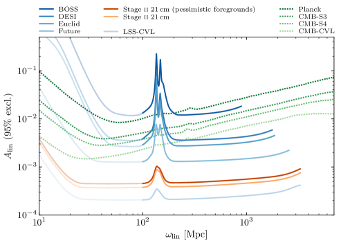
In Figure 16, we provide forecasts for the sensitivity of a suite of cosmological surveys, including Stage ii cm, to primordial features. Since a wide range of feature models can be decomposed into a basis of oscillations which are linear in the wavenumber , we display the estimates of the 95% upper limits for these linear feature models as a function of their frequency . To this end, we added an oscillatory feature with amplitude to the primordial power spectrum of fluctuations,
| (5) |
with pivot scale . We derived the future limits on these inflationary wiggles from the relative power spectrum following Beutler et al. (2019). In particular, we modeled the suppression of primordial power from nonlinear evolution in the Zeldovich approximation based on Seo and Eisenstein (2003) with 50% reconstruction efficiency. Moreover, we separately marginalized over the standard BAO signal and six additional additive and multiplicative polynomial (‘broadband’) terms in redshift bins of width . We also take the effects of the survey window function into account. Due to the robustness of the signal given the analytic insights, we employed wavenumbers up to . (We refer to Baumann et al. (2018a); Beutler et al. (2019) for a detailed description of these forecasts, the treatment of gravitational nonlinearities and further discussion of the estimated sensitivity of future surveys.) Figure 16 shows that a Stage ii cm intensity mapping survey could significantly improve the limits on primordial feature models over currently planned galaxy surveys. In fact, it has the potential to be noticeably more sensitive than a future galaxy survey mapping about objects up to and lead to constraints (or detections) within a factor of a few of a half-sky cosmic variance-limited experiment covering .
The achievable constraints (or detection limits) on these oscillatory features depend not only on the foregrounds, but also our ability to undo the nonlinear ‘smearing’ of structure (due to gravitational evolution in the late universe) by means of reconstruction. Our fiducial choice for the reconstruction efficiency is 50%, which is almost certainly a conservative choice in a foreground-optimist scenario (cf. Karaçaylı and Padmanabhan (2019); Modi et al. (2019b). The mild sensitivity to this assumption is shown in the right panel of Figure 17, while the left panel indicates the weak dependence on the maximum wavenumber . We observe that we can expect measurements that are considerably better than at 95% c.l. over the majority of the relevant parameter space.
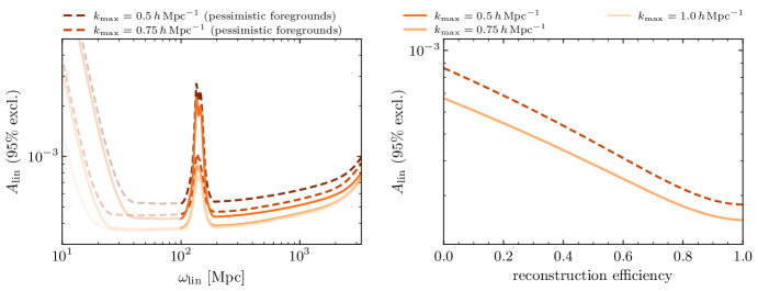
2.7 Primordial non-Gaussianity
One of the exciting targets for future large-scale structure experiments is to obtain evidence for primordial non-Gaussianity (see e.g. Chen (2010); Alvarez et al. (2014); Meerburg et al. (2019) for reviews). In the minimal model of slow-roll, single-field inflation, the primordial density field is perfectly Gaussian. The detection of non-Gaussianity in the primordial field would therefore be immediately informative about the details of the inflationary process.
Observable deviations from Gaussian statistics in the density field are a direct measurement of the particle spectrum and interactions relevant to the inflationary sector. As such, either a detection or an upper limit is testing particle physics at inflationary energy scales, which could be as high as GeV. These energies are unlikely to be probed in collider experiments and thus are the unique domain of cosmological surveys. Furthermore, self-interactions of the inflaton that lead to non-Gaussian signatures are often tied to the fundamental mechanism for inflation itself.
These interactions often lead to a non-zero 3-point function of fluctuations in the primordial curvature perturbation ,
| (6) |
where the Dirac delta-function is imposed by translational invariance and is the bispectrum, which is a function of the triangle configuration of the wavevector arguments. While a Gaussian field has , deviations from Gaussianity lead to non-zero bispectra, whose amplitude is proportional to parameters traditionally denoted as , normalized so that would correspond to non-Gaussianity Chen (2010); Alvarez et al. (2014).555The numerical value of comes from the fact that primordial curvature fluctuations have a root mean square of .
| Single-field slow-roll | Multi-field | |
| Single-field non-slow-roll | Multi-field |
While the amplitude of reflects the strength of an interaction, the shape carries a wealth of additional information about the nature of inflation. The local bispectrum, parameterized by , is a shape for which the signal to noise is dominated by the limit of one of the -modes being soft (i.e. ). This shape is of particular interest since it cannot arise in single-field inflation and would point directly to multiple light fields Maldacena (2003); Creminelli and Zaldarriaga (2004). In contrast, equilateral and orthogonal shapes, with amplitudes and , peak in configurations where and are typical of non-minimal interactions of the inflaton with itself Komatsu et al. (2009). The target thresholds are (see Table 4). With sufficient signal to noise, further information can be extracted either by considering correlation functions beyond the bispectrum or by carefully exploring the scale dependence of the bispectrum Alvarez et al. (2014). In principle, it is possible to extract the spectrum of particles including their masses Chen and Wang (2010); Baumann and Green (2012); Noumi et al. (2013) and spins Arkani-Hamed and Maldacena (2015); Lee et al. (2016), which inspired the name cosmological collider physics Arkani-Hamed and Maldacena (2015).
The best current constraints come from the CMB Ade et al. (2014, 2016) and indicate no statistically significant deviations from Gaussianity. However, the error bars are too large to draw any meaningful conclusions about the primordial dynamics. This motivates us to explore non-Gaussianity in large-scale structure. While future constraints from the CMB are limited by the number of available modes Abazajian et al. (2016) (although large improvements can still be achieved when considering bispectra involving tensors Meerburg et al. (2016)), we have access to a 3D volume of modes with large-scale structure surveys. This is why it is expected that constraints from large-scale structure will eventually become better than those derived from the CMB Alvarez et al. (2014).
In this respect, the cm signal has been identified as unique because it is present throughout the Universe and could provide us with an enormous volume (the entire sky between redshift 0 and ). While non-Gaussianity from cm has been studied in the dark ages Cooray (2006); Pillepich et al. (2007); Cooray (2006); Meerburg et al. (2017) and the epoch of reionization Lidz et al. (2013); Mao et al. (2013); Crociani et al. (2009), our focus in this section will be on the low-redshift universe Tashiro and Ho (2013); D’Aloisio et al. (2013); Camera et al. (2015); Xu et al. (2016); Li and Ma (2017), specifically constraints coming from the proposed Stage ii experiment in the redshift range . We follow the forecasting methodology of Karagiannis et al. (2018). In particular, our forecasts include a comprehensive list of effects, including the bias expansion for non-Gaussian initial conditions up to second order, redshift space distortions, theoretical errors and trispectrum contributions to the bispectrum. We have expanded the codes used for galaxy forecasting to take into account instrumental noise and propagating beam size effects into an effective noise in power spectrum measurements as described in Appendix D. We have further implemented various cuts to simulate the effect of a low- cut and the foreground wedge to simulate our foreground pessimistic scenario.
Our results are summarized in Table 5, where we see that even with conservative assumptions a Stage ii cm experiment could reach at . This target defines a typical level of non-linearity that is inherent in many multi-field models Alvarez et al. (2014). Such a measurement would provide valuable insight into the degrees of freedom that actively produce initial density fluctuations. For equilateral or orthogonal non-Gaussianity, the reach is likely somewhere between the optimistic and pessimistic foreground scenarios. Including the wedge increases the noise, but might not be necessary for constraints on these bispectra. Any measurement of would be incompatible with single-field slow-roll inflation Creminelli (2003); Baumann et al. (2015, 2016). While our forecasts cannot exclude all such possibilities, they would cut out a large fraction of the currently viable parameter space and thus represent an opportunity for a major discovery. It is also possible that Stage ii data could be combined with data from a mission such as SphereX666http://spherex.caltech.edu/, leading to further improvements.
| CMB error | Stage ii cm error | |||
|---|---|---|---|---|
| Planck (current) | CMB-S4 (forecast) | FG pessimistic | FG optimistic | |
| Squeezed (local) | 5.0 | 2.0 | 0.7 | 0.2 |
| Equilateral | 43 | 21 | 27 | 4.5 |
| Orthogonal | 21 | 9.0 | 7.7 | 2.5 |
2.8 Weak lensing and tidal reconstruction
Gravitational lensing affects any map we make of the universe, with the gravitational fields of large scale structure deflecting photons and therefore “re-mapping” the angular coordinates we associate with a given location on the sky. This re-mapping probes the Weyl potential and is thus directly related to the projected distribution of mass between the observer and the source of the photons being measured. Therefore, a reconstruction of this re-mapping, either in terms of a deflection field or a decomposition into magnification and shearing effects, can help to address many of the science goals stated earlier, such as constraining the behavior of dark energy, measuring deviations from general relativity, or determining the masses of light neutrinos which suppress the power spectrum on small scales. A lensing map can further be cross-correlated with other maps of structure, adding redshift resolution and contributing additional constraining power by breaking degeneracies present in individual maps.
Lensing of the CMB has been detected at high significance (e.g. Aghanim et al. (2018b)), and will be one of the main science deliverables of upcoming CMB projects such as the Simons Observatory Galitzki et al. (2018) and CMB-S4 Abazajian et al. (2016). The joint effect of lensing on both CMB temperature and polarization allows for a robust detection in several channels, but since the CMB is effectively a single screen, it only offers access to a single projection of all matter between the observer and the surface of last scattering. Redshift information can be obtained through cross-correlation with other tracers, but this introduces additional populations have associated modeling uncertainties. Lensing can also be measured from the correlations between observed galaxy shapes in a large optical survey (see Ref. Troxel et al. (2018) for the current state of the art). By binning the galaxies in redshift, one can access multiple projections with different redshift weightings. However, there are several pernicious systematics that must be dealt with, ranging from the impact of the telescope’s point-spread function on inferred galaxy ellipticities, to control over the uncertainties in photometric redshifts, to the “intrinsic alignments” of galaxies with their nearby environments (e.g. Mandelbaum (2018)).
In some sense, lensing of cm fluctuations represents the “best of both worlds.” cm intensity maps have angular resolution and other properties that place them in roughly the same regime as CMB maps, so there is promise that the well-developed estimators and pipelines for reconstruction of CMB lensing can be adapted to cm observations. However, since cm maps will be intrinsically three-dimensional, they will also enable the same “tomographic” lensing studies as in galaxy lensing, but free of many of the galaxy-specific systematics mentioned above. The promise of cm lensing has long been recognized in the literature (e.g. Cooray (2004); Pen (2004); Zahn and Zaldarriaga (2006); Metcalf and White (2006); Pourtsidou and Metcalf (2014)), and work from both the simulation Romeo et al. (2018) and analytical Foreman et al. (2018) sides continues.
Of course, that is not to say that cm lensing analyses will not have their own systematics to account for, and these are starting to be investigated. For example, the quadratic lensing estimators that are standard in CMB analyses rely on the Gaussianity and translation-invariance of the intrinsic statistics of the CMB, whereas cm maps will have more complicated statistics that will affect any reconstruction of the lensing map. Refs. Lu and Pen (2008); Lu et al. (2010); Foreman et al. (2018) have shown that these effects will be significant at the redshifts relevant here. Ref. Foreman et al. (2018) has also presented a technique to mitigate a portion of this impact, which will reduce the additive bias on the power spectrum of a reconstructed lensing map, but will generally increase the noise on the same quantity. In cross-correlations between lensing and other tracers, the additional bias will not be present, but the noise will remain, and this must be taken into account when performing forecasts.
However, the bias on the lensing estimator caused by nonlinear clustering is an interesting signal in its own right, being sensitive to the power spectrum of the long density modes that gravity couples to shorter modes within the cm map. (Note that the long modes referred to here are in the same redshift range as the map; lensing also couples long density modes to short modes within the map, but those long modes are at strictly lower redshifts than those being directly observed.) These modes can be reconstructed in the same way as for lensing, a process often referred to as “tidal reconstruction” because it relies mainly on tidal effects Pen et al. (2012); Schmidt et al. (2014); Zhu et al. (2016, 2018); Karaçaylı and Padmanabhan (2019). This method can be used to reconstruct modes with low , which would be obscured by foregrounds if attempts were made to measure them directly. These modes can then be cross-correlated with the CMB to constrain possible integrated Sachs-Wolfe signatures of early dark energy or modified gravity, or cross-correlated with other measurements of lensing to probe structure growth or neutrino mass.
In Table 6, we present forecasts for the total signal to noise on the various auto or cross power spectra related to lensing and tidal reconstruction, applying the forecasting strategy of Ref. Foreman et al. (2018) to the fiducial cm instrument described in Sec. 2.1. The displayed signal to noise is combined over lensing reconstruction from 20 redshift bins spanning , while, for simplicity, we treat LSST galaxies and shear (i.e. galaxy shape correlations) non-tomographically. We also show equivalent values for CMB-S4 lensing, assuming a beam, noise of K-arcmin, and . Even in the case of pessimistic foregrounds, we expect that cross-correlations of cm lensing with LSST can be measured at a precision approaching that of CMB-S4; recall that these cross-correlations will include much more tomographic information than CMB lensing.
For the cm lensing auto spectrum, the “bias-hardening” method mentioned above leads to so much noise that this measurement is not competitive with CMB-S4, even if the foreground wedge can be completely cleaned. However, the power spectra of long density modes in each redshift bin can likely be accessed with very high precision, with a total signal to noise on transverse density modes alone of several hundred regardless of the foreground treatment. In terms of scales, for optimistic assumptions about foregrounds, modes transverse to the line of sight (i.e. with ) can be reconstructed with signal to noise greater than unity for for most of the range between and . With more pessimistic foregrounds, the signal to noise degrades to less than unity above on all scales, although at , signal-dominated reconstruction of modes with will still be possible.
| Quantity / experiment | CMB-S4 | Stage ii | Stage ii |
|---|---|---|---|
| FG pessimistic | FG optimistic | ||
| Lensing LSST galaxies | 367 | 208 | 400 |
| Lensing LSST shear | 178 | 129 | 225 |
| Lensing auto | 353 | 5 | 75 |
| Tidal reconstruction auto | — | 480 | 1281 |
Overall, the signal-to-noise in these measurements is impressive. Following these predictions all the way to their implications for cosmological parameters or specific models of new physics goes beyond the scope of this document, because its main strength will come in particular through interaction of cross-correlations which require assumptions about the existence of other experiments. However, this is a very promising direction to pursue, and warrants further investigation.
2.9 Forward model reconstruction
One advantage of the cm field on the scales relevant to an intensity mapping interferometer is that it is well described by a quadratic Lagrangian bias model Modi et al. (2019b). This allows a forward-model approach to reconstructing modes missing from the observations. Such a reconstruction maximizes the likelihood of a forward simulation to match the observations, under given modeling error and a data noise model, and in simulations it has residual errors lower than shot noise. For redshifts and , ref. Modi et al. (2019b) are able to reconstruct the cm field in simulations with cross correlations on all scales for both optimistic and pessimistic assumptions about foreground contamination and for different levels of thermal noise.
The ability to perform such reconstructions opens up several science opportunities which would otherwise be hindered by foegrounds. First, it lessens the impact of the foreground wedge on BAO reconstruction, tightening the constraints on the cosmic distance ladder by a factor of nearly 2 Modi et al. (2019b). Perhaps more interesting is the opportunities it opens up for correlating with other surveys. The utility of large 21-cm intensity mapping arrays is the highest in the high redshift regime, where there is a lot of cosmic volume to be explored and which is the most difficult to be accessed using other methods. While there are some fields that will cross-correlate straight-forwardly with the cm data, notably the Lyman- forest and sparse galaxy and quasars samples which entail true three-dimensional correlations, any field that is projected in radial direction occupies the region of the Fourier space that is the most contaminated with the foregrounds. Reconstruction techniques allow us to re-enable these cross-correlations and thus significantly broadens the appeal of high-redshift cm experimentation. Two areas which deserve special mention are the cross-correlation of reconstructed cm fluctuations with photometric surveys to measure of the photometric sample and cross-correlation with CMB lensing to constrain the growth rate of structure Modi et al. (2019b).
In Figure 18 we show the performance of such reconstruction. The ability of the forward modeling to reconstruct the information that is completely lost to foreground is remarkable. The exceptional effectiveness of this reconstruction relies partly on the particular recipe that has been used to paint the neutral hydrogen onto dark-matter halos, but realistic complications are unlikely to drastically change these conclusions (see discussion in ref. Modi et al. (2019b)).
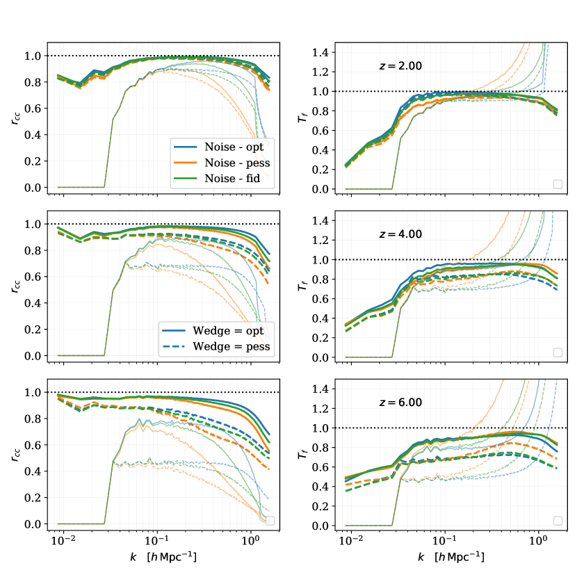
2.10 Basic cosmological parameters: neutrino mass, radiation density, dark energy equations of state
As a natural by-product of measuring the expansion history and shape of the power spectrum, we can improve constraints on many interesting cosmological parameters. While the expansion history is directly sensitive to any of the parameters discussed below, improvements in such measurements often additionally break degeneracies with other parameters so that results in combination with standard datasets such as Planck often improve considerably. The shape of the power spectrum depends coarsely on the matter density and the epoch of the matter-radiation equality through their impact on the transfer function . Additionally, distances in the universe affect the conversion between the observed power spectrum (measured in angles and redshifts) and the comoving power spectrum (measured in inverse comoving distance units), an effect known as the Alcock-Paczynski test Alcock and Paczynski (1979). In practice, redshift-space distortion produce similar effects, which means that they must be modeled simultaneously.
In particular, a Stage ii experiment would provide valuable additional information on:
Neutrino mass. Cosmology is sensitive to the sum of neutrino mass eigenstates (see e.g. Dvorkin et al. (2019)). We know from neutrino oscillation experiments that eV in the normal hierarchy and eV in the inverted hierarchy Lesgourgues et al. (2013); Patterson (2015); Archidiacono et al. (2017); Lattanzi and Gerbino (2018). Massive neutrinos affect the expansion history of the universe and they free-stream out of small scales density perturbations, making the field slightly smoother on scales smaller than the free-streaming length. Their effect can be detected through a particular scale-dependence of the power spectrum between large and small scales, although this usually takes the form of comparing the fluctuation power measured by the CMB with that measured at low redshifts. The general expectation is that the neutrino masses will be detected in the coming years using a number of related methods. The combination of CMB lensing with BAO, the broad-band power measurements in galaxy surveys and weak gravitational lensing of galaxies all have sufficient sensitivity. We expect a Stage ii cm experiment could improve the signal to noise of all these measurements.
Energy density of radiation. The amount of radiation in the early universe is usually parameterized by the effective number777This nomenclature can be misleading because any component with an equation of state like radiation () that is coupled gravitationally will contribute to this quantity. of massless neutrinos (cf. e.g. Green et al. (2019)). Measuring is an important discovery channel for new physics, since any light particle that was in thermal equilibrium with the Standard Model will contribute an additional unless its contribution is diluted by other decays. At the high temperatures thought to be present in the early universe, even very weak interactions are sufficient for thermalization. As a result, percent-level measurements of can be an extremely sensitive and broad probe of new physics (see e.g. Baumann et al. (2016); Abazajian et al. (2016)). Currently, the best measurements arise from a combination of CMB and BAO data, but future cm measurements of the matter power spectrum could help push the CMB measurement to at more than Baumann et al. (2018a).
Dark energy equation of state. While we stress that the main strength of the Stage ii experiment lies in directly measuring the properties of dark energy at high redshifts, it is also capable of determining low-redshift dark energy properties since these change the expansion-history and hence mapping between angles and scales to redshift . As an example, we measure the standard dark energy equation of state parameter , but any model with dynamical dark energy at low-redshift will benefit from these observations of the universe in the pre-acceleration era (cf. e.g. Slosar et al. (2019b)).
These effects are studied though general Fisher matrix formalism, following the methodology of Obuljen et al. (2018). In Table 7, we summarize these forecasts alone and in combination with some standard cosmological probes that will be available towards the end of the next decade. These parameters are the focus of the most important DOE-sponsored upcoming surveys and as such warrant further examination.
| Parameter / combination | LSST + DESI + Planck | CMB S4 | Stage ii+ Planck | LSST + DESI + Stage ii + Planck | CMB-S4 + Stage ii | Everything bagel |
|---|---|---|---|---|---|---|
| [meV] | 38 | 59 | 31 / 27 | 25 / 22 | 24 / 21 | 15 / 14 |
| + 3% prior [meV] | — | 15 | — | — | 14 / 13 | 10.4 / 10.2 |
| [meV] (free ) | 50 | — | 33 / 29 | 26 / 23 | — | — |
| 0.050 | 0.026 | 0.043 / 0.037 | 0.033 / 0.030 | 0.014 / 0.013 | 0.012 / 0.011 | |
| (free ) | 0.017 | — | 0.006 / 0.005 | 0.005 / 0.004 | — | — |
These constraints were derived assuming for 21cm and for DESI (LRGs+ELGs only), and for simplicity and fair comparison no BAO damping in both cases. Note that the higher for cm is justified given its higher redshift and less complex biasing arising from probing less massive halos. Since the non-linear damping of BAO increases with time, our neglect of BAO damping for all surveys overestimates the power of lower-redshift probes. The LSST Fisher matrices were based on the updated work of Font-Ribera et al. (2014), while CMB-S4 Fisher matrices were provided through private communication Meyers (2015). Following Obuljen et al. (2018) we used 5% priors on both and .
2.11 Cross-correlation studies
In the next decade we will see many different probes measure the same volume of space using different tracers and different techniques and cosmology should enter a golden era of cross-correlations. In general cross-correlations are extremely useful for three reasons: (1) any contaminating signal that is not present in both probes will not affect the signal; (2) the value of cross-correlations grows as the number of pairs, i.e. with the square of the number of probes, while the total signal-to-noise in auto-correlations grows only linearly; (3) cross-correlations allow the possibility of sample-variance-free measurements of some quantities, and more generally allow breaking of degeneracies.
In our fiducial experiment, we have assumed a wide redshift range, covering both low redshift and high redshift . These offer different cross-correlation opportunities. At low-redshift the universe will be well sampled by other spectroscopic surveys, allowing us to directly cross-correlate with:
-
•
Spectroscopic galaxy samples. For example, Stage ii has redshift overlap with the DESI BGS (Bright Galaxy Survey) sample at low redshift and with the DESI ELG (Emission Line Galaxy) and LRG (Luminous Red Galaxy) samples in the intermediate redshift range. These cross-correlations will measure the relative bias factors of the samples which would have implications for our understanding of galaxy evolution at these redshfits. Moreover, the large number densities of BGS might allow efficient sample-variance cancellation and perhaps provide a new avenue for constraining non-Gaussianity Seljak (2009) or growth McDonald and Seljak (2009). This is in addition to kSZ cross-correlations discussed in Section 2.12.
On the higher redshift end () our fiducial experiment has been designed to probe volumes not well sampled by other tracers of large scale structure. Nevertheless, there will be avenues for direct cross-correlation, in particular with:
-
•
High-redshift quasars. QSOs have been measured in large numbers by BOSS/eBOSS, but the size of the dataset will gain another considerable boost with DESI. This information will give extra BAO and RSD signal and help calibrate both cm and quasar bias parameters (in conjunction with auto-correlation measurements).
As an example of the science return enabled by the presence of 21 cm data, Figure 19 shows the forecasted 1- error on and the gravitational slip parameter from a combination of spectroscopic data, CMB weak lensing and 21 cm intensity mapping data. While this method is not competitive with methods discussed in Section 2.5, it is arguably less dependent on theoretical assumptions.
-
•
Lyman- forest. The Lyman- forest will have been probed by BOSS, eBOSS and DESI. This cross-correlation will go down to very small scales in the radial direction. Since both probes measure the neutral hydrogen this cross-correlation will help both probes achieve their full potential Carucci et al. (2017). In particular, it will help with measuring the contamination of the Lyman- forest by damped Lyman- (DLA) and high column density (HCD) systems and thus enhance the potential of the Lyman- forest as a probe of a small-scale physics.
-
•
High-redshift forests of other metals. In addition to Lyman-, the high redshift universe also contains other metal forests, like the Siiii, Siiv and Civ forests, whose physics and bias parameters can again be constrained by cross-correlation with cm.
-
•
Lyman- emitters will be detected in large numbers in surveys like HETDEX Hill et al. (2008). Cross-correlations with cm will allow determination of their physical parameters as well as constrain interlopers.
However, more indirect cross-correlations are also possible. The reconstruction method discussed in Section 2.9 will enable cross-correlations with sparse galaxy samples from photometric redshifts and reconstruction of CMB lensing. The lensing field reconstruction discussed in Section 2.8 will enable cross-correlation with both lower redshift galaxy samples and higher-redshift lensing screens (from CMB or EoR intensity mapping Pen (2004)).
In short, it is clear from this discussion that the number of cross-correlations grows quadratically with the number of tracers and hence with the increased number of samples we are entering the era of cross-correlations.
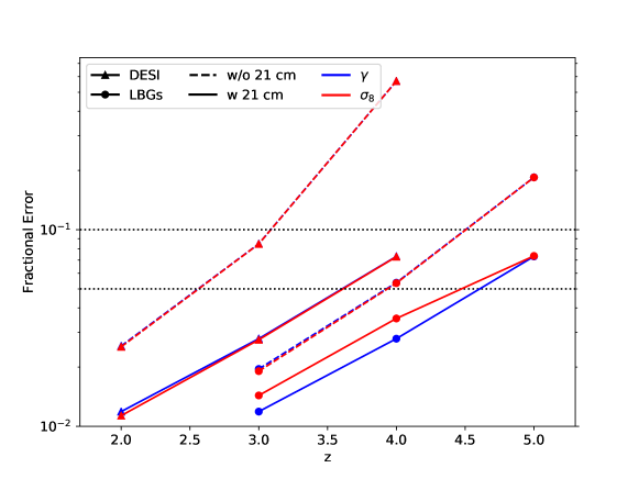
.
2.12 Kinetic Sunyaev Zel’dovich Tomography with Stage ii cm and CMB-S4
Future CMB experiments such as CMB-S4 will have the resolution and sensitivity to produce highly significant measurements of the kinetic Sunyaev Zel’dovich (kSZ) effect, temperature anisotropies induced by the scattering of CMB photons from free electrons with a non-zero CMB dipole in their rest frame. The kSZ temperature anisotropies are correlated with the high-resolution maps of large scale structure produced by a Stage II 21cm intensity mapping survey. Using the technique of Sunyaev Zel’dovich (SZ) tomography, this correlation can be exploited to obtain a tomographic reconstruction of the remote CMB dipole field Terrana et al. (2017); Deutsch et al. (2018); Cayuso et al. (2018); Smith et al. (2018): the CMB dipole observed at different locations in the Universe, projected along the line of sight. 888The primary contribution to the dipole field at any spacetime location is the radial component of the peculiar velocity, however the Sachs-Wolfe and Integrated Sachs-Wolfe contributions are important when considering large-angle or large-redshift correlations. These contributions can be relevant for large volume surveys, as contemplated here. Previous forecasts for kSZ tomography considered galaxy surveys as a tracer of structure, and demonstrated that future surveys such as LSST, in correlation with CMB-S4, can be used to obtain high fidelity tomographic reconstructions of the remote dipole field out to . The reconstructed dipole field can be used to place competitive constraints on primordial non-Gaussianity Münchmeyer et al. (2018); Contreras et al. (2019), modifications of GR Pan and Johnson (2019); Contreras et al. (2019), the growth function Madhavacheril et al. (2019), and various early-Universe scenarios Cayuso and Johnson (2019); Zhang and Johnson (2015). It can be shown Padmanabhan et al. (2019) that using a large redshift coverage has excellent prospects to alleviate astrophysical systematic uncertainties in the resultant forecasts, by combining independent information from multiple tomographic bins. An important property of kSZ tomography is that the measurement of large-scale modes using the reconstructed dipole field can be of higher fidelity than measuring these modes directly from the tracer itself Smith et al. (2018). This feature is particularly relevant in this context, since kSZ tomography probes radial modes which are poorly constrained in 21cm experiments due to foreground contamination.
In Fig. 20, we show the expected signal-to-noise per mode of the reconstructed dipole field using a Stage II 21cm survey and CMB-S4, for different redshift bins. We present two scenarios: the default specifications of the Stage II survey (solid lines), and a configuration where we doubled the size of the array (dashed lines). To produce this forecast, we have used the quadratic estimator of Ref. Deutsch et al. (2018), incorporating the halo model of Ref. Obuljen et al. (2019) for the distribution of HI and the model of Ref. Smith et al. (2018) for the distribution of free electrons. We assume the noise, beam, and sky coverage for CMB-S4 is / / , consistent with the current reference design Abazajian et al. (2019); we have neglected foregrounds and systematics in making our forecast.
The signal-to-noise per mode using the default configuration of Stage II 21cm and CMB-S4 is appreciable over a range of angular scales out to . The dipole field reconstruction can be improved by increasing the angular resolution of the intensity maps. In particular, doubling the size of the array (dashed lines) dramatically improves the reconstruction at . This would allow one to take advantage of the very large volumes probed by a 21 cm survey, as compared to what is possible even with ambitious galaxy redshift surveys. We conclude that a Stage II 21cm survey can be useful for kSZ tomography. Cosmological constraints derived from the reconstructed dipole field would contribute to many of the science goals of a Stage II 21cm survey.
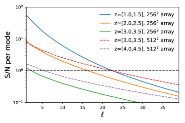
2.13 Direct measurement of cosmic expansion
The measurement of the Universe’s expansion in real time would be a unique confirmation of the standard cosmological model. Cosmological sources drift in redshift with the characterizing time-scale of a Hubble time. Over a 10 year time-span, this results in the redshift change of around . This is challenging both statistically and systematically. However, if measured, it would be one of the very few dimensional quantities that one can measure directly in cosmology999The other prominent examples include time-delays in gravitational lenses that allow us to measure the Hubble rate and the temperature of the CMB.. Controlling absolute redshift calibration at the required level over a decade is extremely difficult, but possible in optical Kim et al. (2015). In radio, however, it should be considerably easier, since clock generators with sufficient accuracy are available off-the-shelf. Since in radio systems the clock-generator sets the absolute time-scale and thus frequency calibration, this (typically dominant) part of the systematic error budget is absent. There are additional subtleties to do with accurate clock transport, or subtle changes in the beam due to changes in the physical state of the reflecting material over 10 years, but while these can produce anomalous changes in the measured signal, they are unlikely to produce systematic shifts.
The basic formula for the redshift drift is given by
| (7) |
where is the Hubble parameter at redshift . In Figure 21, we show a typical prediction for a total drift as a function of frequency for a 5-year experiment. We see that, in principle, the required accuracy is of the order of Hz. If there existed lines whose natural width would be this small, this would have been a trivial measurement. In practice, however, the cm line is velocity smeared to a few 100 km/s giving the natural smoothness of the cosmic signal of around Hz. Thus, one really needs to rely on very precise measurements of the overall structure. On the upside, we see that there is a very definite structure to the shape of this function, so tracing the shift as a function of redshift gives another leverage on systematic control.
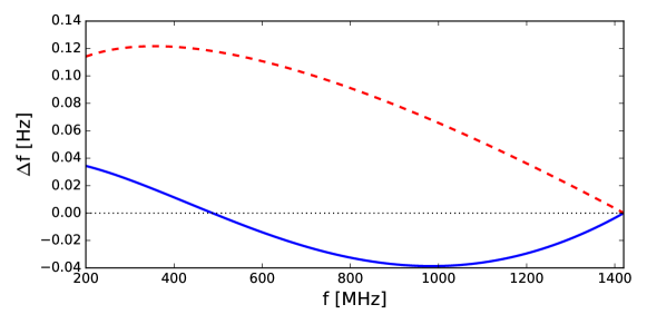
There are two basic approaches to this measurement. The first is to rely on the apparent radial motion of the entire field of density fluctuations. It can be shown that sensitivity of this method is given by
| (8) |
where is the volume of the survey and and are the signal power and noise power (per inverse year of integration) in comoving space respectively and is the radial wave-vector. This expression is correct even when field is non-Gaussian. We see that the majority of the signal is coming from the fine, high frequency radial modes that are suppressed by velocity dispersions in realistic cosmologies. In our numerical work we have found that this technique is not statistically promising for our straw-man configuration, but that it could be for a low redshift array.
An alternative approach is to consider a finite number of cold systems observed in absorption when backlit by distant sources. This has been considered in Yu et al. (2014), which finds a possibility of a detection over 10 years. The forecasting is highly uncertain due to poorly known redshift distribution of radio sources, which is even more poorly known in our redshift range and therefore we do not attempt it in this paper, but a simple extrapolation based on CHIME numbers shows that this measurement would most likely be possible with our Stage ii proposed experiment. However, both methods would require saving data at a radial resolution that is beyond what is necessary for the standard cosmological analysis, and might increase the overall data-storage requirements by a factor of a few.
Finally, we note that in both cases, the scaling is . This very unusually favorable scaling comes from the fact that signal increases linearly with time while noise falls as .
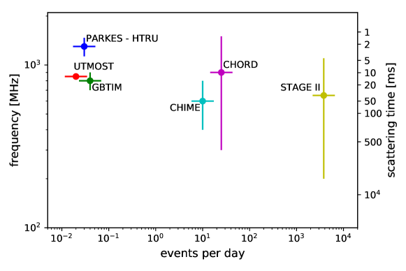
2.14 Ancillary science: Time-domain radio astronomy
1 Fast Radio Bursts: A new cosmological probe
The extremely high mapping speed that makes transit interferometers sensitive to large-scale structure also allows them to detect transients at very high rates Newburgh et al. (2016); Bailes et al. (2017); Amiri et al. (2018). Of particular interest are fast radio bursts (FRBs), a recently discovered and poorly understood class of radio transient Lorimer et al. (2007); Thornton et al. (2013). FRBs are bright, broadband, millisecond flashes, which have now been established to be of extragalactic and cosmological origin Masui et al. (2015); Chatterjee et al. (2017); Tendulkar et al. (2017).
A defining feature of FRBs is that they are highly dispersed: their arrival times depend on spectral frequency due to the frequency-dependent refractive index of free electrons in astrophysical plasmas. This dispersion gives a precise measure of the column density of electrons to the burst source, presenting opportunities to study the distribution of plasma on cosmological scales. The large-scale distribution of plasma is poorly understood since it mostly resides at densities and temperatures where it does not significantly emit or absorb radiation. These so-called “missing baryons” have only recently been detected for the first time through stacking analyses of the thermal Sunyaev-Zel’dovich effect Tanimura et al. (2019); de Graaff et al. (2019). Beyond providing a better understanding of structure formation, a precise measurement of the electron distribution would aid in the interpretation of the kinetic Sunyaev-Zel’dovich (kSZ) effect. The kSZ effect measures a degenerate combination of the electron power spectrum and of large-scale velocity flows. Independent information about the electron distribution would permit the velocity flows to be disentangled, providing a check on the theory of dark-matter structure formation, a probe of the nature of gravity on large scales, and constraints on modified gravity models.
McQuinn (2014) proposed measuring the plasma distribution from a sample of FRBs by stacking their dispersion measures on foreground optically-detected galaxies. The contribution to the dispersion measure from the FRB hosts, as well as the redshift-dependent contributions from interloping plasma, can be separated from the signal using its dependence on impact parameter. Such an analysis requires relatively precise sky localizations to significantly better than an arcminute for the FRBs. This could be achieved by adding a number of low-cost outriggers to the array providing km baselines.
A second, related method is to measure the 3D clustering of FRBs directly using dispersion, and thus electron column density, as a proxy for radial distance and redshift (Masui and Sigurdson, 2015). FRBs themselves are likely to be biased tracers of the large-scale structure, however, their measured clustering will be distorted by systematic errors in their radial distance measurements from structure in the line-of-sight plasma. These dispersion-space distortions can then be exploited to precisely measure the plasma distribution.
The proposed experiment operates at a factor of three lower frequency than most FRB discoveries to date, despite some moderately sensitive searches in this band (Chawla et al., 2017). Only very recently have FRB discoveries at 400 MHz been announced Boyle (2018), and as such the rates and detectability at low frequencies are highly uncertain. At these frequencies, the effects of scattering of the burst signals by inhomogeneous plasma are expected to make them more difficult to detect (although the presence of this scattering helps in interpreting discovered bursts Masui et al. (2015)).
To get a back-of-the-envelope event rate, we proceed as follows. We assume that of the currently measured FRBs, the total signal bandwidth is usually around . Hence we take the Stage ii experiment to be effectively three independent experiments operating between 200 – 400 MHz, 400 – 700MHz and 700 – 1100 MHz. We then assume the same instrument properties as described in Appendix D (including sky-noise, etc) and assume that the FRB brightness distribution is Euclidean calibrated to observed CHIME event rate of 5/day. This gives approximately 3500 events per day. Over the five year span of the experiment, this would produce around 6 million FRB detections. While this number is uncertain at a factor of a few, the reality can be better as well as worse. More information is given in Table 8.
| 200 – 400 MHz | 400 – 700MHz | 700 – 1100 MHz | |
|---|---|---|---|
| Bandwidth | 200 MHz | 300 Mhz | 400 MHz |
| Total System Temperature | 120K | 75K | 65K |
| Instantaneous FOV | 91∘ | 27∘ | 10∘ |
| 10- threshold fluence | 26 mJy ms | 13 mJy ms | 6 mJy ms |
| Event rate in FOV | 1200/day | 980/day | 1300/dat |
It is clear that such large sample would be transformative for the field, as it would start to approach the number of galaxies in a typical galaxy survey (DESI will, for example, measure redshifts of some 30 million galaxies).
2 Pulsars: alternative probe of modified gravity
Pulsars are highly magnetized neutron stars that, due to their anisotropic emission and rapid spinning, are observed as lighthouse-like periodic sources that can be used as astrophysical clocks. The extraordinary precision of these clocks permits their use in pulsar timing arrays to search for gravitational waves with light-year wavelengths, as would be emitted by the mergers of super-massive black holes Arzoumanian et al. (2018); Taylor et al. (2015); Shannon et al. (2013). In addition, the extreme compactness of neutron stars permits precision tests of general relativity in the strong gravity regime by tracking the dynamics of multi-body pulsar systems using pulsar timing Taylor and Weisberg (1989); Kramer et al. (2006). These opportunities to test fundamental physics depend on the discovery of new highly stable millisecond pulsars or pulsars in exotic dynamical systems.
Like FRB searches, pulsar searches can benefit from the high mapping speed of transit interferometers. The proposed experiment covers the 200 to 1100 MHz band, which includes part of the spectrum that has been identified as promising for finding the millisecond pulsars (Stovall et al., 2014) that permit searches for gravitational waves and the most precise tests of general relativity. Current state-of-the-art surveys have searched large fractions of the sky, with a few minutes of integration time, using telescopes with order of collecting area. Current algorithms for searching for pulsars in collected data require that data to be contiguous in time. As such, a transit interferometer can only integrate down in sensitivity for the duration of a transit which, for the proposed 6 m dishes and 70 cm wavelength, is roughly 27 minutes for a source at the equator and longer at higher declinations. It would take roughly 15 days to survey most of the sky to this depth, at which point the square kilometer of collecting area and 27 minutes of dwell time would permit the discovery of pulsars 1000 times fainter than current surveys.
In addition, recently proposed algorithms permit the coherent co-adding of observations taken on consecutive days Smith (2016), meaning the integration time on a given patch of the sky could be dramatically increased. Depending on the efficacy of these algorithms, which has not yet been demonstrated, this would permit the detection of sources fainter by a few orders of magnitude.
Compared to future surveys, the proposed experiment will be 300 times more sensitive than CHIME, 64 times more sensitive than HIRAX, and 6 times deeper than the maximum depth of FAST (even in a 10-year survey, FAST could only reach its maximum depth over a small fraction of the sky, whereas we are proposing to reach this depth over the full sky). The SKA, having a similar timeline and comparable collecting area, will have a comparable maximum depth. However, due to the non-compact configuration of the SKA antennas, it will only be able to survey a small fraction of the sky to this depth.
However, beyond discovery, Stage iiwill be able to continuously monitor the SKA discovered pulsars. The SKA1-LOW and SKA1-MID arrays will detect of the order of pulsars Keane et al. (2015). It is clear that none of the current telescope facilities, including SKA itself, would have enough sky time to follow up the majority of these discoveries. Due to the daily monitoring of a significant subset of these pulsars (depending on the pointing), Stage ii will be complementary to SKA. With its unprecedentedly high timing cadence, Stage ii will be able to characterize each of these new pulsar discoveries, and carry out a systematic study of pulsar temporal variabilities, including nulling, glitches, sub-pulse drifting, giant pulse emission, and potential signatures of new fundamental physics.
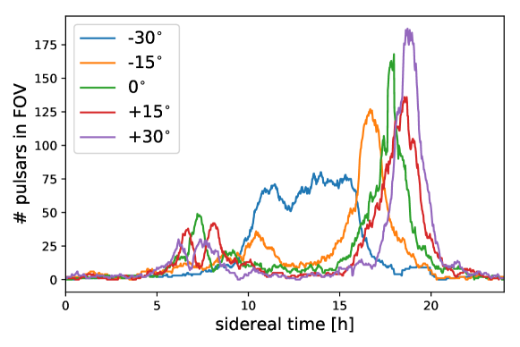
3 Challenges and opportunities
While cm intensity mapping provides an efficient means of measuring large scale structure to high redshift, the instrument and analysis must be designed to overcome systematic sources of contamination: terrestrial radio signals from human-generated radio frequency interference (RFI) and the Earth’s ionosphere, and extremely bright astrophysical synchrotron foregrounds from our own galaxy. The former can be addressed with suitable site locations and benefits from RFI mitigation and ionospheric characterization work from current low frequency instruments. We can address the latter by using the inherent spectral smoothness of the foregrounds to separate them from the cosmological signal. However, this places stringent requirements on frequency-dependent instrument calibration, and foreground removal becomes a key design driver for instrument characterization, stability, and uniformity. A baseline instrument configuration that can achieve foreground removal and sensitivity limits sufficient for the science goals outlined in the previous sections will require that we build a highly redundant array of order 65,000 uniformly-spaced feeds, allowing fast-Fourier transform (FFT) beamforming for data correlation and compression, operating across a redshift range of (200-500 MHz), and utilizing real-time gain calibration. As noted below, storing the full correlation matrix is not practical, but beamforming this number of detectors as a method of data compression is possible with present-day computation resources, although it requires real-time calibration that has not yet been demonstrated with current instruments. This input from current experiments is critical to assess the trade-offs between raw sensitivity and ease of calibration. Achieving foreground removal requirements with a sensible analysis strategy can only occur with a concerted R&D effort along three directed paths, described in more detail throughout this section:
-
•
Technological: The primary technological development paths to build and calibrate the instrument baseline design described above (with the capability to remove foregrounds and enable data compression) include improved signal processing and digital conversion electronics; optimized RF analog chain design with an emphasis on uniformity; and gain stabilization and beam characterization instrumentation.
-
•
Analysis: The primary analysis path is to build on the foreground removal and RFI mitigation techniques from current generation experiments and develop FFT beamforming compression and associated instrument design specifications to enable analysis at an achievable computation scale.
-
•
Simulations: The primary simulation path is to build synthetic data for Development and Deployment, Validation and Verification, and Uncertainty Quantification. This must include full instrument characteristics to optimize instrument design and fully explore cosmological parameter constraints, particularly for analysis involving cross-correlations and other survey data. The minimum required inputs to form a sky map for this process are mock catalogs with galactic foregrounds and point sources. By the time this project becomes reality, our understanding of the low-frequency sky will be considerably improved from Stage i and Epoch of Reionization experiments.
In Section 3.1 we review the outstanding design requirements for cm cosmological mapping, heavily informed by the experience of the current generation of experiments. In Section 3.2 we summarize the main technological R&D areas to address these, and then describe specific technology advances in more detail. In Sections 3.3 and 3.4 describe the analysis and simulations challenges, respectively. Finally, in section 3.5 we relate the technical needs of a cm experiment to historical DOE strengths and capabilities, as well as pointing out opportunities for growth.
3.1 Design Drivers and Requirements

Using radio surveys of galaxies to probe the BAO scale and constrain dark energy has a long history in the literature (see Rawlings et al. (2004) and references therein). It was realized more than a decade ago Peterson et al. (2006); Rawlings et al. (2004) that low resolution radio telescopes in an ‘intensity mapping mode’ could be sensitive to redshifted neutral hydrogen with enough resolution to be resolve the BAO signature and could be used to transform constraints on Dark Energy and other cosmological parameters. The first measurements were made on large, steerable dishes, choosing a survey region which overlaps with high-redshift galaxy surveys, allowing a detection of highly redshifted neutral hydrogen via cross-correlation Chang et al. (2010); Masui et al. (2013); Switzer et al. (2013). Following on this success, new radio interferometers have been built that are dedicated to measuring neutral hydrogen at high redshift, in principle overcoming the limitations of a single dish measurements at higher redshifts. In this section, we outline the primary design drivers for a cm cosmology survey instrument. Experience from current generations of experiments already taking data (HIRAX, CHIME, LOFAR, PAPER, HERA, MWA, and Tianlai among others – see Figure 24) has shown that the most challenging requirements come from a tackling bright astrophysical foregrounds. The experiments populate a wide space of instrument configurations, and the largest instrument on the sky in the phase-2 redshift range is CHIME Bandura et al. (2014, 2016); Berger et al. (2016); Newburgh et al. (2014), which has chosen a cylindrical dish design to give the instrument a wide field of view in one direction, but which requires an intricate calibration scheme Berger et al. (2016). Below we outline the design drivers for a Stage ii experiment, but it should be emphasized that foreground contamination is almost always setting the requirement, and adequately removing it must include dedicated efforts across all of instrument design, data analysis, and simulation.
Astrophysical Foregrounds. Astrophysical foregrounds, primarily synchrotron emission from the galaxy and unresolved point sources, have much higher intensity than the cosmological signal of interest. These foregrounds have a smooth spectral shape and hence can in principle be distinguished from the cm emission from large scale structure Procopio et al. (2017); Pober et al. (2013); Seo and Hirata (2016); Liu and Tegmark (2012). However, any frequency dependence in the instrument response, for example from the instrument beam or gain fluctuations, can complicate our ability to differentiate between the smooth foreground and the essentially Gaussian cosmological signal Shaw et al. (2015, 2014). Removing these foregrounds drives design choices including element uniformity, array redundancy, assessment of instrument stability and stabilization methods; provides opportunities for new calibration techniques in both beam and gain measurements; and requires analysis and simulations to fold in calibration measurements and assess their impact on cosmological parameter estimation.
Instrument Calibration. Work in cm calibration focuses on instrument gain and beam measurement for the goal of removing astrophysical foreground power. Simulations for CHIME have provided a scale to the problem: the instrument response on the sky (‘beam’) must be understood to 0.1%, and the time-dependent response of the instrument (‘gain’) must be calibrated to 1% Shaw et al. (2014, 2015). Current instruments rely primarily on sky signals for both types of calibration, however this has not yet been demonstrated to adequately remove foregrounds with these instruments. Throughout this chapter we outline design choices to meet uniformity and stability specifications that must be carefully integrated into the instrument design, verified during testing and deployment, as well as develop or advance new methods of calibration for this removal.
FFT beamforming requiring real time calibration and array redundancy. The correlation cost and data rate from the Stage ii array will require implementing an FFT beamforming correlator. Such correlators use FFT-based sampling of the interferometric geometry Tegmark and Zaldarriaga (2009) to reduce the computational correlation cost from order to and output data volume from to order . Taking advantage of this technique requires that all elements of the array be redundant (that their beams are similar), placing stringent requirements on element uniformity. In addition, this correlation will be performed in real time, and so this requires that we employ real-time calibration to account for instrumental changes (or that the instrument remains extremely stable). This technique will be attempted on current generation telescopes, and we expect work on those experiments will inform requirements and algorithms for Stage ii instrument.
Environmental considerations. In addition to astrophysical foregrounds, two sources of terrestrial signal contaminants must be eliminated or otherwise mitigated: human generated radio-frequency interference (RFI) and Faraday rotation in the ionosphere.
Radio bands within the cm redshift range are popular as communications frequencies. This forms a bright RFI signal at discrete frequencies within our measurement band. RFI can be reduced or eliminated by a suitable choice of radio-quiet observation site such as the middle of South Africa or western Australia Offringa et al. (2015), which are remote areas with limited communications in countries with suitable infrastructure. Even if RFI must be removed, various experiments operating in locations with high degrees of interference, notably LOFAR (located in the Netherlands), have built impressive RFI removal techniques Offringa et al. (2012) that the Stage ii experiment can draw from.
The ionosphere is a plasma and acts in concert with the Earth’s magnetic field to rotate the polarization vector of incoming light. The rotation is proportional to as well as the number of free electrons present in the ionosphere, which vary across all time scales. While the cosmological signal is unpolarized, most foreground emission from the galaxy is polarized, and so this adds a time variable component to the foreground characterization and removal. The dependence means it is not expected to impact the shorter wavelengths (frequencies above 500 MHz, ), but it will impact longer wavelengths relevant to a Stage ii experiment. Work towards measuring and removing this rotation using accurate maps of the magnetic field and GPS data to infer free electron content is ongoing for experiments at long wavelengths. Because signal propagation through the ionosphere is critical for satellite telecommunications, it is well modelled and current low frequency radio telescopes are working to remove signal variability from the ionosphere Arora et al. (2015).
Required Sensitivity. Instrument noise stems from a combination of intrinsic amplifier noise (noise temperatures for state-of-the-art radio telescopes range from 25 K cryogenic to 100 K uncooled) and sky brightness temperature (which span between 10K - 1000K depending on pointing and frequency). Because synchrotron emission increases at lower frequencies, at high redshifts (above 3) the system noise is dominated by the sky and no longer by the amplifier, thus improved noise must be achieved by fielding more antennas rather than better performing front-end amplifiers. In the absence of systematic effects, detecting the cm signal requires fielding instruments including thousands of receivers to achieve mapping down to the mean brightness temperature of the cosmological cm signal of 0.1 - 1 mK in the redshift range within a few years.
Computing Scale. Radio astronomy has always been at the forefront of ‘big data’ in astronomy. Current generation cm instruments produce of data per day without any compression, natively generating an amount of data where is the number of elements (currently ), representing challenges in data reduction, transfer, storage, analysis, distribution, and simulation. Compression by a factor of is achievable by exploiting redundancy within the interferometer, but requires the use of real-time, in-situ calibration and places strong constraints on the uniformity of the optics between elements. For the straw-man experiment with (65k) elements, this compression would reduce the data rate from per day to per day, but still produce a data set that is over a multi-year observation campaign. To aid in data transport, analysis, and data quality assessment, we plan to compress our data further, co-adding maps into a weekly cadence. This reduces to data size but increases pressure on real-time instrument calibration. In addition, to enable transient science we will need fast triggers, already deployed at current generation instruments.
3.2 Technologies Enabling Science
Understanding the instrument requirements illustrated above allows us to identify dedicated, targeted, and coordinated research and development areas that will enable a cm Stage ii experiment sufficient for the science case presented throughout this document. We propose a multi-pronged development effort: early digitization for improved stability and uniformity, optimizing the analog radio receiver elements, and new methods in beam and gain calibration.
1 Early digitization and signal processing
Most generally gain refers to the scaling between the incoming signal and the digitized signal, typically from the analog system (feeds, amplifiers, cables) and digitizer. Analog components are subject to gain variation, typically due to temperature changes, as the signal travels from the focus of the dish to the later digitization and correlation stages. As noted above, gain variation is one of the limiting factors in removal of astrophysical foreground power. One avenue of development is to digitize directly at the focus of the dish because signal information is “vulnerable” at all points along the analog stages, so the imperative is to digitize as early as possible, after which the signal is (nearly) “invulnerable”. The resulting digital signal has more resiliency against time-variable changes in the signal chain (while some of these are simply moved from analog signal transfer into the clock distribution, the latter is inherently narrow-band), offers the possibility of more flexibility in calibration injection signal algorithms to make gain solutions more robust, and allows us to use commodity or other well-established protocols developed for timing and data transfer. However, this comes at the expense of overcoming the RFI from the digitization in the field, potentially increased cost, and will require all amplification to occur at the focus and thus we may find we need carefully designed amplifiers and thermal regulation at the focus as well.
Several technology developments make receiver electronics with integrated digitizers (early digitization) a promising technology for cm projects. Critical components that are now available commercially include:
-
•
Room temperature amplifiers with noise temperatures below sky brightness requirements from 100MHz to 1.2GHz.
-
•
Low cost digitizers operating in the gigahertz regime with up to 14-bit resolution are readily available. This allows a trade-off: high bandwidth direct digitization provides the ability to oversample and design high performance digital band selection filters and high order frequency equalizers, but analog conditioning is simpler to implement and model. The final design will be decided by cost trade-offs while still meeting stability requirements for foreground removal.
-
•
Low cost programmable logic devices capable of interfacing with a high-speed ADC, providing digital filtering to the frequency range of interest, and interfacing to high speed networks.
-
•
Similarly, the availability of integrated RF / ADC / FPGA devices in the near future may provide a path to very compact high-performance receivers.
By digitizing at the focus we broaden the possibilities for instrument calibration, bandwidth, and signal processing, however there are a few additional considerations:
-
•
As noted, one of the technical challenges for cm telescopes is the need for 1% gain stability over at least 24 hours. The primary culprits of gain variation with temperature come from the amplifiers and any analog transmission (either coaxial cable loss or radio-frequency-over-fiber). By digitizing at the focus, the analog transmission is unnecessary and then any variation will be dominated purely by the amplifiers. The resulting temperature variation can be either mitigated by use of thermal regulation of the circuitry at each dish focus or removed by injecting a calibration signal, or both. Because noise diodes have a gain stability of C, achieving the required gain stability still requires thermal regulation of C. Amplifiers have roughly similar thermal regulation requirements, however they are more difficult to decouple from the environment because they are either connected or embedded in the antenna. Thus, development should be placed towards building calibration sources, digital or otherwise, to enable gain stabilization.
-
•
We must isolate the sensitive RF input with signals in the -100dBm range from the high power digital outputs from the ADC which typically operate near 0 dBm. In addition, RF radiation from the digital processing system must be shielded from the input and from any other antennas.
-
•
The raw data rate from the digitizer is large, a few 10Gbit/second. This can be substantially reduced depending on the oversampling level, with digital filtering in the FPGA that receives the digitizer data, followed by transmitting only the bandwidth containing useful physics data. For some correlator architectures it may also be useful to transmit data separated by frequency band to an array of correlation processors. The system can trade off oversampling at a few gigahertz and digitally filtering down to the band of interest for a more complex analog system. In theory a digital filter can do significantly better than an analog filter in terms of stability and out of band rejection, and may become more cost effective on the time scale of the Stage ii instrument.
-
•
There must be a very precise clock distribution system sent out to each of the digitizers. This moves the instrument phase calibration problem from the analog system into the clock distribution system. Numerous techniques exist for synchronizing a distributed clocking system, and these must be adapted to enable a low cost calibration system. This has been found to be challenging even with the digitizers in only two locations, and so carefully designing and testing this timing system, including mitigations and estimates for cable reflections, will be a critical R&D task for any distributed digitization across the instrument.
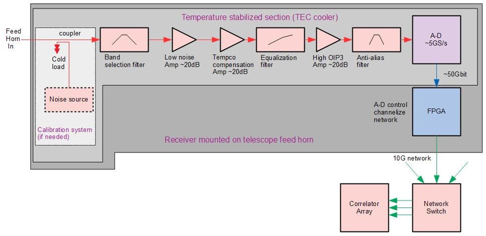
2 Analog design
Optimization of optical design.
Most existing and near-future cm experiments, e.g. CHIME Bandura et al. (2014), Tianlai Chen (2012), HIRAX Newburgh et al. (2016), and HERA DeBoer et al. (2017), all have chosen parabolic reflectors with the receivers supported at the focus with metal legs, leading to some diffraction and reflections. To illuminate the dish, they have also designed variants of dipole receivers with wide beams that have non-negligible cross-talk and frequency-dependence. These choices are typically made as a cost- and complexity savings, but make calibration more difficult. Further study for optimization, including options such as off-axis geometries (like SKA-mid and ngvLA) and possibly horn/Gregorian receivers, will be important particularly since many of those experiments will have greater experience with the parabolic reflector geometries in the near-term. These experiments also span a range of wavelength-to-size ratios and we would use these experiments along with simulations to form a specification on the dish diameter. Wide bandwidth optical systems are under development. See Figure 26. The optimization would include keeping marginal costs low while also meeting uniformity and bandwidth flatness specifications, and exploring new dish fabrication techniques (such as using a fiberglass-based design Hovey et al. (2015), see Figure 27).
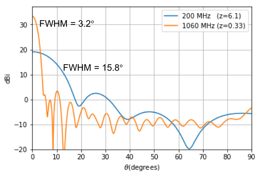
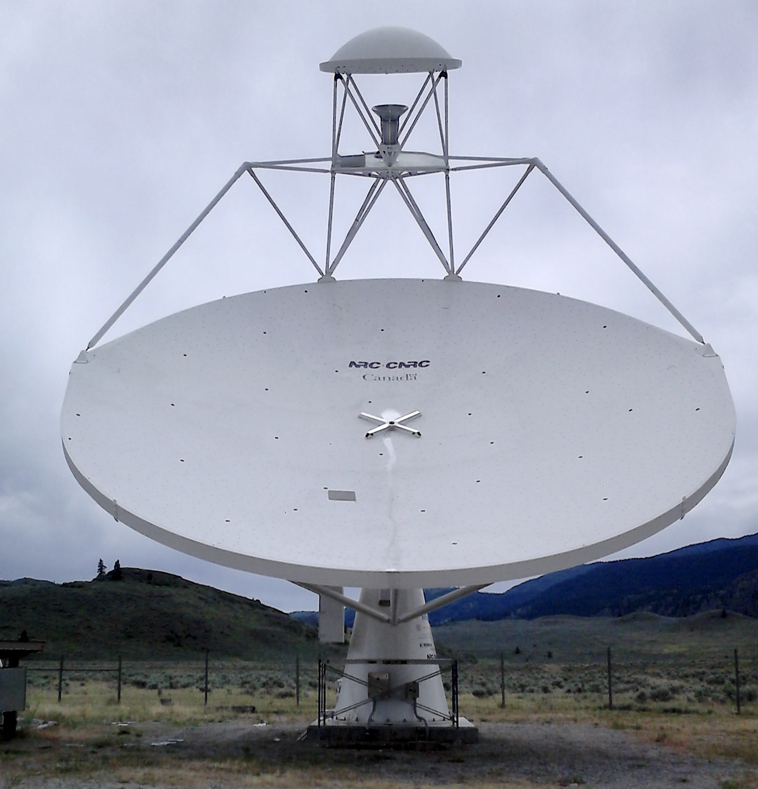
Front-end sensitivity and bandpass.
When properly designed, the receiver noise temperature is dominated by loss in the analog feed as well as the noise in the first stage amplification. HIRAX has chosen to reduce the system noise by up to 30% by fabricating the first stage amplifier directly in the antenna itself, reducing the transmission loss and taking full advantage of low-noise transistors available in these bands. In addition, current generations of cm experiments DeBoer et al. (2017) have found that their bandpass shape is a limitation of their foreground removal, and are actively working on new feed designs that have a more carefully shaped bandpass. One development path for the active circuitry in the HIRAX feed would be to add additional RF circuitry to flatten the bandpass to remove ripple and other features, allowing an easier path for foreground removal. This introduces more stringent oscillation conditions on all amplification stages to reduce the possibility of amplifier oscillation and we will learn more about the feasibility of this technique for mass production as additional prototypes are fabricated for HIRAX.
Uniform interferometric elements for calibration and FFT correlation. Similar interferometric baselines should see the same sky signal and so differences between them can be used to assess relative instrument gains over time. This technique is known as ‘redundant baseline’ calibration and has been developed as a method of meeting the gain stability requirements Liu et al. (2010); Carilli et al. (2018); Dillon et al. (2018); Ram Marthi and Chengalur (2014); Dillon and Parsons (2016); Sievers (2017). This requires both a decision to space the interferometer dishes the same distance apart, and also have highly uniform interferometric elements. Most cm instruments have chosen their baseline spacing to use this technique, however have been limited by the fact that their interferometric elements are not identical enough to achieve precision calibration. To overcome this, we would investigate dish fabrication tolerances required for this calibration as well as how we might use new dish fabrication techniques (for example, fiberglass dishes with embedded mesh conductors, currently being prototyped for SKA and HIRAX, see Figure 27) to meet these needs.
In addition, the requirements that we use FFT or similar beamforming Pen (2004); Tegmark and Zaldarriaga (2009, 2010); Masui et al. (2017) to compress that data forces stringent requirements on the uniformity of response, beam shape, mechanical construction and alignment, gain control, etc. across what will ultimately be on the order of 65k detector copies. The requirements for this uniformity and how to achieve it will be part of the instrument design process.
3 Instrument Calibration
Gain Stability. Each antenna has a characteristic response to an input sky signal, which varies with both time and frequency, known as the instrument gain. The frequency-dependent gain for each input must be known to 1% on time scales between the integration period (s scales) and a few hours (depending on the frequency of on-sky radio calibrator sources) Shaw et al. (2015). The two primary techniques for achieving this are to design an instrument which is inherently stable enough to meet this specification or to design a calibration plan which can ensure we meet this specification, or (ideally) both. CHIME Bandura et al. (2014); Newburgh et al. (2014) is updating a classic radio noise-injection scheme which can be used to calibrate many signal chains at once. To implement such an active calibration technique for dishes will require development of stablized transmission algorithms and may be made easier with early digitization and development of calibration sources which may be independently fielded at the focus or flown on a quadcopter drone. We will also require passive models of gain and beam variation with temperature and dish pointing. This modeling is essentially standard for radio telescopes and precision modelling has been demonstrated with at least one instrument (CHIME).
Beam Characterization. Each antenna also has a characteristic response on the sky, known as the instrument beam. Because this response (main beam and sidelobes, as well as polarization) is capable of mixing frequency dependence and sky location, it is expected to be the primary source of contamination from foreground emission into the signal band, and so must be known even more accurately than the gain (0.1%) Shaw et al. (2015). This level of calibration is difficult for cm telescopes because they are stationary and designed to have large beams for improved survey speed Sokolowski et al. (2017). In addition, some instruments (such as CHIME) have large dish sizes which can be difficult to model and simulate, requiring exceedingly detailed knowledge of support structures and surface mesh. Many cm instruments are beginning to use quadcopter drones to map the beam shape (HERAJacobs et al. (2016), SKAVirone et al. (2014); Pupillo et al. (2015), LOFARChang et al. (2015)) and while this technique seems promising to meet the needs for cm cosmology it is unlikely we will be able to measure all of the beams from all of the dishes in an instrument with 65k dishes, and so this beam calibration requirement also forces a specification on uniformity in dish fabrication.
4 Data flow and processing
Computing requirements for a 65k-element interferometer come from both the correlation burden and the data reduction, transfer, storage, analysis, and synthetic data production. For the correlator computation, we will need to pursue development in computing approaches which can improve the cost scaling both for equipment and power. Examples could include using commodity-hosted FPGA’s, using/developing dedicated ASIC’s D’Addario and Wang (2016), or GPUs to smoothly take advantage of the fast-paced hardware updates for correlator computation.
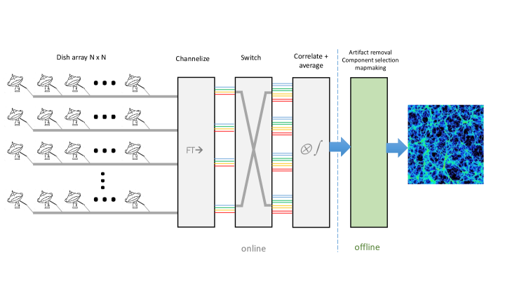
3.3 Data Analysis
Releasing science deliverables for the community from a cm experiment depends crucially on developing and deploying, including validation and verification, an analysis pipeline that can ingest vast quantities of data and transform it into well characterized frequency maps and power spectra. This is a computationally costly and varied exercise, but does not require continuous real time processing, and thus can be performed at an external high performance computing site. We can divide the analysis up into three broad areas discussed below.
Flagging, Calibration and Pre-processing at scale. In this area
the data is processed to reduce the remaining systematics which may
effect our ability to access the cosmological signal.
Of particular importance is cleaning of any RFI by flagging times and frequency channels that have been contaminated. This is a well understood problem within radio astronomy (Offringa et al., 2012), though the effects of residual RFI at the small level of the cm signal is only starting to be addressed (Harper and Dickinson, 2018).
Though much of our calibration must be done in real-time (see 3.1) to enable FFT correlation, there are still degrees of freedom that must be corrected, particularly degeneracies that may not have been fully fixed (including but not limited to an overall gain scale for the entire observation, (Liu et al., 2010)), and calibration of the bandpass (the array-wide frequency dependent gain). Again these are problems that are well understood within radio astronomy.
Astrophysical Foreground Removal. Along with the sensitivity requirements for measuring a faint signal, the key analysis problem for cm intensity mapping is the need to remove contaminants that are many orders of magnitude larger than the cosmological signal. Though foreground cleaning is a common problem across cosmology, the required dynamic range is unique to cm intensity mapping.
In principle the foregrounds can be separated from the signal using their smooth frequency dependence (Seo et al., 2010). However, even an ideal instrument couples anisotropy in the astrophysical foregrounds into spectral structure with an amplitude generally significantly larger than the cosmological signal. This extremely challenging problem is called mode-mixing and is exacerbated by instrumental systematics such as gain variations and optical imperfections which must be minimised (see the discussion in Section 3.1). There exist in the literature many proposed techniques to separate the cosmological signal from the foregrounds, but these have only demonstrated success in simulations.
Foreground mitigation falls broadly into two classes: foreground avoidance and foreground cleaning. Foreground avoidance is the simplest of these two approaches, relying on the fact that contamination produced by a typical interferometer configuration is strongest in certain regions of -space (see Appendix C). Producing cosmological results only using the cleanest modes is a simple and effective technique. This technique, however, becomes deeply unsatisfactory at low frequencies, particularly in the dark ages. Here galactic synchrotron and extragalactic point source radiation quickly becomes very bright, typically hundreds of Kelvin at , even at high galactic latitudes. At the same time the window of clean modes dramatically narrows due to the relative scaling of the angular diameter distance and Hubble parameter with redshift Pober (2015). Combined, this means that at a given threshold for contamination we exclude increasingly large regions of -space at high redshifts, significantly degrading any cosmological result.
Foreground cleaning instead of (or in conjunction with) foreground avoidance then becomes an attractive option. A general feature of foreground cleaning methods is that they rely on detailed knowledge of the instrument response to predict and subtract the actual foreground signal. For instance, given perfect knowledge of the complex beam of each individual antenna, a tomographic map of the sky can be effectively deconvolved to remove the spectral structure induced by the instrument’s beam. The residual contamination is set by both the amplitude of the raw contamination and the accuracy with which the beam has been measured. This is similar in spirit to the residual temperature-to-polarization leakage produced by mismatched beams of orthogonal polarizations in CMB -mode searches, which can be accurately predicted and removed given beam measurements despite the fact that the CMB temperature anisotropy “foreground” is orders of magnitude larger than the -mode signal.
Cosmological Processing. Having cleaned the foregrounds out of the data we then need to process it to quantities useful for cosmology such as power spectra and sky maps. Though this has been done within the CMB and LSS communities for many years, the fact that we are dealing with radio interferometric data after foreground cleaning brings unique challenges. The source of these is that the measured data is abstract: it is a complex, spatially and spectrally non-local measurement of the sky. This adds significant complexity in generating maps and power spectra from the data, but also tracking which modes have been measured (and which are missing) to allow us to accurately measure uncertainties. Regardless, we expect to be able to significantly draw on the conceptual frameworks used for cosmological data analysis to be able to tackle these problems Shaw et al. (2015); Liu et al. (2014a); Jewell et al. (2004).
Although we can create a broad outline of how the analysis pipeline, and we are able to draw on many mature and well understood techniques, there are several areas that will require research investment to ensure the success of a large scale cm intensity mapping survey.
Scaling. While we can draw on existing techniques for all stages of the analysis, a significant challenge is scaling these to be able to work with the vast increase in data that we will generate in an energy-constrained/post-Moore’s computing landscape. This will require optimizations in algorithms and implementations to reduce the computational cost of the processing, and ensuring that the techniques can scale in parallel to run on leading edge supercomputers.
Systematic Robustness. Both astrophysical uncertainties (such as the exact nature of foregrounds) and instrumental uncertainties (such as calibration and beam optics) cause foreground contamination. Developing more robust cleaning techniques will reduce systematic biases, but potentially allow us to reduce the instrumental tolerances leading to cost savings.
Improving signal recovery. Significant numbers of modes are lost to foregrounds, which reduces our constraining ability generally, but particularly affects science that needs access to the largest scales. Improved foreground removal that reduces the effect of the wedge could improve this, as would methods like tidal reconstruction Zhu et al. (2016, 2018); Foreman et al. (2018), but these techniques need substantial development. Similarly, traditional reconstruction techniques Eisenstein et al. (2007); Padmanabhan et al. (2009) that recover non-linear modes need work adapting them for the peculiarities of cm intensity mapping.
3.4 Simulation Needs and Challenges
The challenges facing cm surveys are significant but, at least to , well understood. However, our ability to tackle them requires a sophisticated approach to overcome them both through instrumental design and offline analysis. It is therefore essential to use simulations to close a feedback loop that allows us to predict, and thus refine, the effectiveness of a design and analysis strategy.
Producing realistic simulations of data from any instrument configuration and propagating these to final cosmological results is a conceptually straightforward prospect:
-
1.
Produce a suite of full-sky maps of the “true” sky, with one map per frequency and at each frequency bin observed by the instrument. There are a variety of approaches to form full-sky maps of the signal and foreground, and full exploration of the data should include common sky models to include other observables (e.g. galaxy surveys) for form estimates of cross-correlations.
-
2.
“Observe” these maps with a simulation pipeline that contains sufficient realism to capture any and all non-idealities that might produce contamination in the data.
-
3.
Feed these mock observations into the data analysis pipeline discussed in the previous section, and the same pipeline that would be used on real data, and produce reduced data and cosmological analyses.
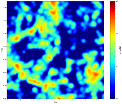
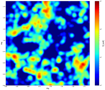
For verification of foreground removal effectiveness gaussian or pseudo-Gaussian cm simulations are largely sufficient Alonso et al. (2014); Shaw et al. (2015). However, for targeting sensitivity to specific effects (e.g. non-Gaussian initial conditions), or in cross-correlation with other probes, more accurate simulations constructed from mock-catalogues will be required. This allows us to produce correctly correlated maps for additional tracers (e.g. LSST photometric galaxies), and also for radio point source contribution to the foregrounds.
Though the relation between HI density and total matter density involves complex environment dependent processes, simulating it can be done efficiently. Recent work has shown that one can take advantage of the fact that neutral hydrogen in the post-reionization era resides almost entirely inside dark matter halos (Villaescusa-Navarro et al., 2018). It is possible to combine the presently available HI data to constrain an analytical halo model framework for the abundance and small-scale clustering of HI systems (Padmanabhan et al., 2017; Padmanabhan and Refregier, 2017). Thus, one can calibrate the relation between dark matter halos and HI using hydrodynamic simulations and create 21cm maps via less expensive methods such as N-body or fast numerical simulations like Pinocchio Monaco et al. (2013), ALPT Kitaura and Heß (2013), HaloGen Avila et al. (2015), EZMock Chuang et al. (2015), PATCHY Vakili et al. (2017), COLA Tassev et al. (2013), QuickPM White et al. (2014), FastPM Feng et al. (2016), or Peak Patch Stein et al. (2019). It may even be possible to adopt a simple perturbation-theory-inspired approach Modi et al. (2019b), which would allow very large volumes to be simulated very efficiently.
As the dominant foreground contribution, simulating the galactic synchrotron must be done with care to ensure that the simulations are not artificially easy to clean. A simple approximation can be produced by proceeding from a full sky map at a radio frequency (typically the Haslam radio survey map at 408 MHz) and scaling this map to different frequencies based on the known spectral index of galactic synchrotron radiation. However this is not sufficient at the dynamic range between the foregrounds and the cm signal and we must be careful to include: spectral variations about a pure power law; small scale angular fluctuations not captured in existing surveys; and polarization, including the effects of emission at a wide range of Faraday depths which generates significant spectral structure in the polarized emission Shaw et al. (2015). More sophisticated galactic models, for example from MHD simulations, could also be developed and used here.
Regarding (2), a realistic instrument simulation pipeline would take the maps discussed and convolve them with the complex beam for each antenna in the interferometer. This can be done by direct convolution utilising the fact that for a transit telescope it is sufficient to generate a single day of data. However for wide-field transit interferometers this can be more efficiently performed in harmonic space using the -mode formalism ( instead of ). Some of the required code would be similar and could in principle built upon similar codes used in the CMB science, such as the TOAST package101010http://hpc4cmb.github.io/toast/intro.html using fast numerical techniques for beam convolution Prézeau and Reinecke (2010).
For these simulations we need to generate realistic simulations of the telescope beams. Electromagnetic simulation codes such as CST, GRASP and HFSS can be used for this, but achieving the accuracy required is challenging computationally Cianciara et al. (2017); Deng and Campbell-Wilson (2017); Ewall-Wice et al. (2016). An alternate approach is to generate synthetic beams with sufficient complexity to capture the challenges posed by real beam, these are computationally easier to produce, but must be informed by real measurements and electromagnetic simulations to ensure their realism, and may be aided by machine learning algorithms.
Capturing non-idealities in the analog system, particularly gain variations, is mostly straightforward as these can be applied directly to the ideal timestreams. Additionally we need to include time-dependent beam convolution (including position and brightness) for temporally varying sources such as solar, jovian and lunar emission as well as the effects of RFI at low levels Harper and Dickinson (2018).
Including calibration uncertainties poses a particular challenge, because of the realtime calibration and compression of the instrument, simulating these effects requires either: generating data at the full uncompressed rate, applying gain variations, and then performing the calibration and compression processes; or the computationally easier alternative of generating models of the effective calibration uncertainties.
After the first two stages, mock observations are then fed to the proposed data analysis pipeline, and propagated through to final cosmological products, to assess analysis systematics, instrument design, real-time calibration, and data processing to determine whether the pipeline is sufficient to meet our science goals.
Though the simulation program is well defined, there are already many open challenges discussed below.
Understanding the HI distribution. To map the HI distribution to the cosmologically useful matter distribution requires cutting edge hydrodynamic simulations to capture the small halos that HI favours over a cosmologically interesting volume. This additionally improves the efficiency and accuracy with which we can produce mock skies.
Scale. To assess and understand a proposed design we need to be able to produce large numbers of emulators that Monte-Carlo over the experimental uncertainties. The number, size and complexity of these simulations requires a large scale effort to plan, generate and manage them.
Improving the Feedback Loop. While a straightforward version of the simulation loop above can tell us whether a proposed design does or doesn’t meet our needs, it does not tell us how to improve the design to ensure that it does. For a complex instrument with many design parameters is is essential to be able to guide this process by using simulations to infer the most relevant combinations of changes.
3.5 Relation to DOE capabilities
This chapter has enumerated the technology and analysis challenges for studying cosmic acceleration by mapping the large-scale structure of the universe using cm radiation. As with other large DOE-HEP experiments, it requires data from imperfect detectors to be turned into useful scientific output by application of multi-level calibration schemes that incorporate the as-built instrument characteristics and thorough end-to-end numerical simulation of the physics of the measurement process. DOE has a unique heritage in successfully constructing large experiments of this type, making it a particularly appropriate home for the development of a cm intensity mapping experiment. Capabilities found in the DOE Laboratory complex in technical, computing, and management categories are discussed below.
Technical capabilities. DOE has long experience with RF systems for its hadron and electron accelerators. Hardware for manipulating RF modes to efficiently couple sources to accelerator waveguides and cavities has much in common with the matching optics used for radio telescope receivers. High channel-count, fast RF digitization and processing is also used extensively in control and beam diagnostics. Large accelerators such as LCLS-II can include over a thousand channels of RF front ends and high-performance digitizers connected to a distributed data network. Although optimization of dynamic range, bandwidth, and noise characteristics differ from those needed for the cm experiment, many commonalities between the designs remain.
Data acquisition systems at large HEP and photon science experiments generate enormous volumes of digital data that must be transported over networks that may comprise tens of thousands of high-speed links. Data transport, real-time processing, and interface to commodity server farms requires DAQ developers to have specialized expertise in the most modern microelectronics families (ASICs, FPGAs, optical transceivers, etc.) and to be aware of rapidly advancing trends that open opportunities for greater performance in future projects. The Front End Link Exchange (FELIX) and global Feature Extractor (gFEX) platforms being developed for the ATLAS experiment are examples of state-of-the-art hardware coming out of the DOE labs; evolved versions of such platforms can find very direct applications in real-time cm signal processing.
Table 9 shows a comparison of data rates in some current and future experiments drawn from HEP, photon science, and radio astronomy. Data rates in the cm Stage ii experiment proposed here, although challenging, are not out of the range of some of the more ambitious projects shown.
| Experiment | Data rate | Year | Note | Ref. |
|---|---|---|---|---|
| [GB/s] | ||||
| VLA | 0.3 | 2013 | Resident Shared Risk Observing mode | VLA |
| ALMA | 1.8 | 2021 | Overall | ALM |
| LHC | 25 | 2018 | Average rate, all 4 experiments after triggering | LHC |
| LSST | 6.4 | 2022 | Peak rate | LSS |
| LCLS | 10 | 2009 | CXI instrument | Thayer et al. (2017) |
| LCLS-II | 320 | 2027 | High frame-rate scattering detector | LCL |
| XFEL | 13 | 2017 | 2D area detector | XFE |
| SKA1 | 8,500 | 2022 | Overall | SKA |
| CHIME | 13,000 | 2017 | Input to F-engine | CHI |
| 21cm Stage ii | 655,000 | 2030 | Input to F-engine |
Computing capabilities. All stages of developing this experiment will require the involvement of large computing facilities. The full system simulation as well as actual data processing will require high-performance computing and efficient storage, handling and processing of data volumes in the petabyte range. This can be efficiently addressed through existing and planned infrastructure facilities within the DOE laboratory complex that will also drive new developments in network connectivity between DOE sites. DOE runs NERSC, one of the world’s largest high-performance computing systems, ALCF and ORCF (limited access) and has put significant investment into exascale computing across all centers. It also hosts two CERN Tier-1 data centers.
In addition to challenges presented by the data volumes alone, there are massive algorithmic challenges that can be efficiently addressed using existing DOE structures present within Advanced Science Computer Research (ASCR) and SciDAC. On the simulation side these includes running large simulations of the universe. On the data analysis sides, the calibration problems and foreground removal problems can be recast in terms of large-scale linear solvers, error analysis, kernel estimation, machine learning, etc. These problems will benefit from developments in the current exascale initiative and work that has been done on hybrid compute architectures that can be particularly efficient ith large data rates.
Management capabilities. A cm Stage ii experiment will need to follow organizational models similar to those that have evolved in DOE’s other recent HEP programs. These may include coordination with other agencies and/or international partners, setting up scientific collaborations and a formal structure responsible for executing the project plan, and arranging for appropriate levels of oversight. During the construction phase, test systems for quality assurance and metrology will be essential for mass-produced components to meet performance requirements. Predecessor projects such as US-ATLAS/CMS silicon detector modules, LSST focal plane raft towers, and CMB-Stage 4 detectors and readout will provide useful models and lessons. Finally, DOE has experience in organizing collaboration-wide scientific activities to generate high-fidelity simulations of system performance. The LSST Dark Energy Science Collaboration’s Data Challenges are a recent example. As stated earlier, it will be absolutely essential to perform end-to-end simulations for a cm Stage ii experiment.
Current DOE laboratory efforts. There are currently several small path-finder efforts at various labs not directly funded by DOE HEP.
At BNL, a small test-bed experiment, BMX, has been set-up operating at 1.1-1.5GHz. It has been taking data since Fall 2017 in single dish mode and was upgraded to a 4 dish interferometer in the Summer 2019. The results are promising despite the experiment being situated at the lab site, which is an extremely poor location in terms of RFI. Early science results include characterization of out-of-band emission from global navigation satellite services that will act as a potential systematic for low-redshift cm experiments. As a test-bed, the system will be used to test various approaches towards beam and gain calibration and to gather on-sky data from early digitization prototypes. It will thus continue to provide a convenient bridge between laboratory testing and a test deployment on a real radio telescope which often involves significant travel costs and limited time allocation.
The Fermilab Theoretical Astrophysics Group has been closely involved with cm intensity mapping for the past decade. Early work included forecasting and technical design studies for cm arrays Seo et al. (2010) and development of analysis techniques Shaw et al. (2015, 2014). Currently, with NSF support, the group hosts the Tianlai Analysis Center (TAC), which analyzes data for the Tianlai instrument in China. The current, “Pathfinder” version of Tianlai includes an array of 16, 6-meter diameter dishes and 3, 15 m x 40 m cylinder telescopes operating in the 650-1420 MHz range and acts as a useful test-bed instrument for future efforts Das et al. (2018). Near-term goals include determining the optimal design of future arrays (cylinders, dishes or both), and detecting HI at low and high redshift ( 0.15 and 1.0). The effort includes data storage, calibration, RFI removal, data quality assessment, mapmaking, power spectrum analysis, and development and testing of the Tianlai analysis pipeline. These tasks are partly enabled by the substantial computing resources at Fermilab’s Scientific Computing Division.
4 cm measurements beyond redshift
In this document we have so far talked about the cm intensity mapping as mapping of the aggregate emission from many unresolved galaxies. However, this is a correct picture only in the universe at redshifts lower than , where the universe is mostly ionized with a few pockets of neutral hydrogen residing in galaxies.
Going to earlier times and higher redshifts, we encounter two distinct regimes. The epoch between and is also known as the Epoch of Reionization. During these periods, first-generation stars and galaxies were formed and begun the process of reionizing the universe. This process is highly non-linear and driven by astrophysics rather than cosmology. This epoch experimentally interesting, because the signal is boosted by large region of completely ionized “bubbles” residing in sea of otherwise largely neutral hydrogen. Therefore, significant effort is dedicated to measuring this regime and we describe it in the Section 4.1.
Going even further, to redshift higher than , we see the universe as it was before the formation of the first stars. The pristine hydrogen, untainted by the messy start and galaxy formation promises the ultimate frontier, but it is experimentally daunting as we discuss in Section 4.2.
4.1 Cosmic Dawn and Epoch of Reionization
cm techniques have been used for studying the Cosmic Dawn and the Epoch of Reionization (EoR). A number of experiments such as HERA DeBoer et al. (2017), PAPER Parsons et al. (2010), LOFAR van Haarlem et al. (2013), MWA Tingay et al. (2013), and GMRT Paciga et al. (2013) are seeking to make the first measurements of how the first luminous objects affected the large-scale distribution and ionization state of hydrogen. While these efforts target a currently unexplored phase of galaxy formation, they do not have P5 goals as primary science and thus we are not proposing these for consideration by the DOE. However, they do have indirect relevance to the goals outlined in this roadmap, for two reasons. First, these experiments may detect signatures of exotic physics that are relevant to P5 goals, provided these signatures cannot be easily be explained by CDM, even when allowing for extreme astrophysical scenarios. Second, these experiments face many of the same technical challenges as the experiments proposed in this roadmap, and thus any breakthroughs on either side in instrumentation, observation, or data analysis will be mutually beneficial.
A prime example of possible exotic physics would be the recent results from the EDGES experiment Bowman et al. (2018). EDGES has claimed a first detection of a large dip in spectral energy distribution of the cosmic radio monopole at around MHz, corresponding to if this is due to the line. While such an absorption feature is predicted by most theories of Cosmic Dawn, the dip measured by EDGES is anomalously large, implying hydrogen gas that is considerably cooler than is allowed by CDM or an additional source of background besides the CMB Feng and Holder (2018). This discovery has yet to be confirmed, and there are some concerns related to the foreground modeling Hills et al. (2018). However, if true, it would present a remarkable measurement which has already generated considerable interest within the high-energy physics community. The EDGES result, if validated, could potentially point to the first hints of interactions between baryons and the dark sector Fraser et al. (2018); Barkana et al. (2018); Berlin et al. (2018); Barkana (2018); Slatyer and Wu (2018); Hirano and Bromm (2018); Neufeld et al. (2018), or place constraints on the primordial power spectrum Yoshiura et al. (2018), relic neutrino decays Chianese et al. (2019), dark energy Costa et al. (2018); Hill and Baxter (2018), axions Moroi et al. (2018); Houston et al. (2018); Sikivie (2018), interactions between dark matter and dark energy Wang and Zhao (2018), dark matter annihilations D’Amico et al. (2018); Yang (2018); Cheung et al. (2019), decaying dark matter Clark et al. (2018), primordial black holes Clark et al. (2018); Hektor et al. (2018), fuzzy dark matter Lidz and Hui (2018), and warm dark matter Safarzadeh et al. (2018); Barkana (2018); Schneider (2018).
Fundamentally, a experiment aims to make large, three-dimensional maps of the distribution of hydrogen, regardless of the epoch it is probing. Thus, breakthroughs with Cosmic Dawn and EoR experiments also represent breakthroughs for any experiment described within this roadmap. In this respect, discoveries like the EDGES result could potentially be significant steps forward. A confirmed EDGES detection would be analogous to the first measurements of the CMB blackbody spectrum, while follow-up measurements of the spatial fluctuations of the line would be analogous to the first measurements of CMB anisotropies. Just as with the CMB, such measurements would herald the beginning of a new standard probe of cosmology.
4.2 Dark Ages
After recombination111111Recombination is really a misnomer for this epoch since protons and electrons were never combined before. Primordial combination might be a more appropriate phrase. of hydrogen, when the Cosmic Microwave Background (CMB) was created at redshifts around , the universe was completely neutral, with neutral hydrogen the dominant component. As matter continued to cluster in the post-recombination universe, peaks in the matter density were enhanced and eventually led to the formation of the first generation of stars and galaxies, which emitted radiation capable of reionizing the ambient neutral hydrogen. Between recombination and the formation of the first stars, there is a high-redshift epoch that is ideal for the cosmological mapping of density fluctuations through intensity mapping, during which hydrogen is neutral and and traces the overall matter distribution. This epoch is generally referred to as the Dark Ages.
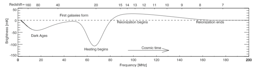
Several physical details prevent the mapping of density fluctuations over the entire redshift range from recombination and reionization. For instance, when , residual free electrons from recombination provide a coupling between the CMB and the temperature of the hydrogen gas through Compton scattering. In turn, collisions drive the spin temperature (which quantifies the relative number of hydrogen atoms in the ground versus the excited hyperfine state) to the gas temperature. With the CMB temperature in equilibrium with the spin temperature, there is no net absorption or emission from the line, and therefore no signal to observe. At , Compton scattering becomes inefficient. The spin temperature and the gas temperature remain coupled to one another, but together decouple from the CMB temperature. The gas then cools adiabatically as , in contrast with the CMB’s cooling as a , which results in a net absorption signal. This continues until , at which point the neutral hydrogen is sufficiently dilute that the collisional coupling between the gas temperature and the spin temperature become ineffective. Direct absorption of emission of photons then couples the CMB temperature to the spin temperature once again, and the signal disappears. The observed brightness temperature of the 21 cm signal as a function of redshift is shown in Figure 30.
A redshift window in the range could potentially be used for intensity mapping and would provide large-scale maps of pristine density fluctuations. There are several advantages to doing so. First, the regime is too high in redshift for the first luminous objects to have formed yet, and therefore the signal is driven by cosmology rather than astrophysics. Second, the signal is not Silk damped, and thus density perturbations can in principle be mapped to extremely small scales (with perhaps the Jeans scale being the only limitation). Third, these small-scale structures are still in the linear regime at such redshifts, making theoretical modeling efforts considerably simpler than analogous efforts for galaxy surveys. Finally, the volume of our observable Universe that falls in the range is substantial, leading to exquisite statistical errors on parameters.
1 A new window into the Universe
In the CMB, well-understood linear processes are sufficient to relate observed anisotropies in temperature and polarization to energy density perturbations generated during the early universe. This is what makes the CMB such a powerful probe of fundamental physics, limited mainly by diffusion damping Silk (1968) that erases anisotropies (and therefore primordial information) on small scales. On the other hand, lower-redshift large scale structure in principle offers many more accessible modes, but a large portion of these modes is affected by nonlinear processes that are difficult to model. These nonlinearities are less severe at higher redshift: in particular, before the first collapsed objects formed at , the limiting scale is the Jeans scale, Mpc-1 Ali-Haimoud et al. (2014). Since the number of linear modes scales as the cube of the maximum linear wavenumber, observations at this epoch hold great promise for increasing our knowledge of fundamental physics.
The only observable available to us during this epoch is the cm hyperfine transition of neutral hydrogen.121212There is also a hyperfine transition in deuterium nuclei, corresponding to photons with wavelength cm. In principle, this is observable with the same interferometers designed for cm, and would yield a pristine measurement of the primordial deuterium abundance, but will be a much more challenging observation than cm Sigurdson and Furlanetto (2006). The theory of the high-redshift cm signal is very well understood Loeb and Zaldarriaga (2004); Lewis and Challinor (2007), and for most purposes is well described by linear perturbation theory Ali-Haimoud et al. (2014). From a practical standpoint, the signal, which is in absorption against the CMB back-light, will be very hard to observe for many reasons that are similar to those that hinder the detection of cm emission at lower redshifts. In addition, a cm photon originating at these very high redshifts will redshift into the low MHz wavebands, which will be hard to observe from the ground due to reflection by the ionosphere. It is estimated that this limitation becomes significant for (MHz Jester and Falcke (2009)), and any signal beyond that would require an experiment outside of the ionosphere, such as in space, or, as has been proposed in Refs. Burns et al. (2017); Jester and Falcke (2009); Wolt, et al. (2013), on the far side of the moon.
This certainly implies that any measurement will be very far in the future. For this reason, we will not suggest a specific experiment (which would come with a unique set of limitations), but instead remark upon the general potential of an experiment targeting these observations, that would inevitably build on the progress made with lower-redshift detections. Simply put, the high-redshift cm signal will provide a three dimensional window into the linear Universe, providing access to of order more modes than the CMB131313Assuming independent redshift slices in this redshift range, each with for Loeb and Zaldarriaga (2004).. This tremendous amount of statistical power makes cm measurements from the Dark Ages the ultimate probe of the conditions in the early Universe. Exquisite constraints could be expected on many quantities of interest Loeb and Zaldarriaga (2004), such as the scalar spectral index Adshead et al. (2011) and primordial non-Gaussianities Pillepich et al. (2007); Muñoz et al. (2015); Meerburg et al. (2017).
Before we present a unique science target, let us briefly highlight two observables discussed earlier, namely primordial features (Section 2.6) and non-Gaussianities (Section 2.7), that a probe of the Dark Ages could significantly improve.
The detectability of features at high reshifts depends critically on the amplitude, frequency and scale-location of the features, as well as the angular and redshift resolution of the experiment. Forecasts show Chen et al. (2016) that a cosmic variance limited cm experiment measuring fluctuations in the redshift range with a 0.01-MHz bandwidth and sub-arcminute angular resolution could potentially improve bounds by several orders of magnitude for most features compared to current Planck bounds. At the same time, cm tomography also opens up a unique window into features that are located on very small scales ( Mpc-1).
Besides features in the power spectrum, the same physics generally produces features in all primordial correlation functions. The cm field as a probe of non-Gaussianities, and the bispectrum in particular, has been explored in Ref. Xu et al. (2016). Of particular interest is the possible detection of massive particles in the early Universe. Heavy particles with higher spin can leave distinct features on higher-order correlation function Baumann et al. (2018b); Lee et al. (2016). The signal is predicted to be very small, but a detection would present the first evidence for a mass hierarchy as predicted by string theory Arkani-Hamed and Maldacena (2015). Because of the smallness of the signal, cm has been suggested Meerburg et al. (2017) to provide the only realistic observable to constrain the presence of these particles. We refer to Ref. Meerburg et al. (2017) for details of the models that could potentially be observed with cm.
Now, we will present a single example that is rather unique, concerning the potential signatures of primordial gravitational waves in fluctuations of the observed cm intensity. We describe these signatures below, and provide estimates for their constraining power on the amplitude of gravitational wave power left over from the early Universe.
2 Gravitational tensor modes
One of the holiest grails in our attempt to understand the physics of the early Universe is the possible detection of primordial gravitational waves. These can be generated by the same early-universe process that generates the seeds for the (scalar) density fluctuations that we observe in the CMB and large scale structure. Within the paradigm of inflation, the expected level of primordial gravitational waves generated during inflation is measured with respect to the production of scalar fluctuations by a relation of the two primordial power spectra:
| (9) | |||||
| (10) |
In single-field slow-roll inflation, some of the parameters above are related by , , and . Here and are two slow-roll parameters, which are proportional to the second and first derivative of the scalar potential, respectively, and are required to be much less than unity for inflation to last a sufficient time to solve the horizon and flatness problems Guth (1981). In more complicated models, including those with multiple fields, deviations from slow-roll, and non-canonical kinetics, these relations will be altered, pick up additional degrees of freedom, or break altogether. The relation between the scale dependence and the amplitude of primordial waves is particularly interesting. A deviation from a red spectrum would indicate a violation of the null energy condition, and suggest the spectrum was not generated from the vacuum (see e.g. Cook and Sorbo (2012); Namba et al. (2016)), or could rule out inflation as the source of gravitational waves Khoury et al. (2001).
Current attempts using the B-mode polarization signal in the CMB aim to detect as low as Abazajian et al. (2016), providing an interesting science target in terms of the field excursion during inflation Lyth (1997). Unfortunately, it is quite possible given the nature of , which effectively describes the energy scale of inflation, that the actual level of primordial gravitational waves is orders of magnitude below . Measurements beyond this level will be difficult using CMB B-modes, mostly due to B-modes generated through lensing of E-modes, which obscure primordial B-modes at the level of for ground-based observations. Delensing methods can mitigate a large fraction, but this becomes increasingly hard for smaller values of . Furthermore, for very low values of , patchy screening and scattering of CMB photons around reionization can generate B-modes which will be hard to disentangle (although the maps could in principle be de-screened Meerburg et al. (2017)) from primary B-modes. Many other probes of primordial gravitational waves face significant challenges. For example, direct detection using interferometers (e.g. LIGO and (E)LISA) is unlikely given the relatively small scales probed by such experiments Meerburg et al. (2015), and methods utilizing the polarized Sunyaev-Zel’dovich effect require very low noise levels in the CMB and an exquisite measurement of free electrons in the Universe Alizadeh and Hirata (2012).
Measurements of large-scale structure during the Dark Ages will be affected by a gravitational wave background in several ways, and observations over a large enough volume have the potential to see these effects at high significance. We will highlight two such effects here:
-
1.
Tidal fossils: After a large-scale tensor mode enters the horizon, it will induce a specific kind of inhomogeneity into the statistics of the density field, similar to what happens with the tidal field generated by scalar perturbations at second order. While the original tensor mode will decay with time, its imprint on large-scale structure will not, leaving behind a “fossil” that can be detected at later times using an appropriate estimator Masui and Pen (2010); Schmidt et al. (2014); Masui et al. (2017). The power spectrum of this estimator is directly connected to the primordial tensor power spectrum, and therefore to the tensor-to-scalar ratio, with constraining power scaling with the inverse of the number of observed modes. Ref. Masui and Pen (2010) has argued that a Dark Ages survey could use this effect to constrain to the level.
-
2.
Curl lensing: Like density fluctuations, gravitational waves can affect the paths of photons as they travel through the universe. Unlike density fluctuations, however, gravitational waves generate a curl component of a reconstructed deflection field. The potential of these curl modes as a probe of gravitational waves has been studied e.g. in Refs. Dodelson et al. (2003); Li and Cooray (2006); Book et al. (2012); Chisari et al. (2014); Sheere et al. (2017). The constraining power of this method also scales with the inverse of the number of modes, and in Ref. Book et al. (2012) it was argued that in principle a measurement of curl lensing from the Dark Ages could provide a constraint as low as .
A full treatment of all effects induced due to the presence of large-scale tensor perturbations, including the two effects above, was performed in Refs. Schmidt and Jeong (2012); Schmidt et al. (2014). Observationally, it is not evident that all of these effects can be easily separated. In our forecast below, we will assume that tidal fossils and curl lensing can be distinguished. We hope to report in the near future to what extent these effects can indeed be separated (for example, through bias-hardened estimators, as recently explored in Ref. Foreman et al. (2018) for the case of scalar lensing).
We consider a Dark Ages cm survey over , corresponding to a comoving volume of roughly . The number of modes is set by the maximum observable wavenumbers along and perpendicular to the line of sight, and , and we assume that the statistics of these modes are amenable to theoretical predictions at the necessary precision. We assume sufficient frequency resolution to access the Jeans scale in the line-of-sight direction, . In the transverse direction, we map into the corresponding baseline that can observe that wavenumber. This mapping is redshift-dependent; for the tidal fossil forecast, we evaluate it at since this is where the signal to noise peaks. For the curl lensing forecast, we split the survey into four equal redshift bins, evaluate the mapping (and any other relevant redshift-dependent quantities) at the midpoint of each bin, and combine the separate forecasts from the different bins. Note that is not necessarily the longest baseline present in the instrument, but rather the maximum baseline at which all shorter modes are signal-dominated.
For tidal fossils, we adopt the quadratic estimator from Ref. Masui et al. (2017), using their expression for the estimator noise with the survey properties given above. For curl lensing, we use a modification of the formalism from Ref. Foreman et al. (2018), which simply amounts to a change in filters applied to the observed cm fluctuations. We ignore nonlinearities in the cm field, which will slightly degrade the signal to noise at the longest baselines we consider. The ability to detect lensing is affected by shearing of coordinates at the source redshift by gravitational waves present at that redshift; we incorporate this “metric shear” in our forecasts, following Ref. Dodelson et al. (2003).141414Important differences between our forecast and that of Ref. Book et al. (2012) include the incorporation of metric shear, which degrades the signal to noise, and the use of a fully 3-dimensional formalism that accounts for correlations caused by long modes along the line of sight. The curl lensing power spectrum is computed using a modified version of CAMB Lewis et al. (2000), and we compute the cm brightness temperature power spectrum following Ref. Muñoz et al. (2015).
In Fig. 31, we plot the minimum value of detectable at 3 by either method, assuming that primordial gravitational waves are the dominant signal in each case. We have also indicated the levels at which other effects begin to dominate the primordial signal. For curl lensing, vector perturbations generated at second order by primordial scalar perturbations produce the dominant signal if Saga et al. (2015); Saga (2016). Contaminants in the tidal fossil estimator have not been extensively investigated, but tensor perturbations generated by second-order scalar couplings have been found to enter other observables at the level of (e.g. Baumann et al. (2007)), so we take this to be the relevant floor.151515These second-order contributions can be exactly computed once the amplitude of scalar perturbations is known, and could then be subtracted from a measurement of tidal fossils or curl lensing to access values of smaller than the floors we have quoted. However, cosmic variance will prevent us from obtaining sufficiently precise measurements for this procedure to work. Our forecasts do not include cosmic variance; in other words, for each maximum baseline, we have computed maximum values of for which the null hypotheses of “no tidal fossils” or “no curl lensing” could be rejected at . If is below either of the quoted floors, a rejection of these null hypothesis will not inform us about the value of .
We find that an interferometer with baselines of at least a few hundred kilometers would be able to constrain to the level of , equivalent to the target for CMB-S4, with even larger arrays being able to beat this target. Such arrays are clearly a highly ambitious notion, but currently represent the only feasible way to detect primordial gravitational waves at a lower level than CMB-S4. At the extreme limit of feasibility, an array covering a large fraction of the Moon’s surface (corresponding to a maximal baseline of km, the Moon’s diameter), could in principle detect as low as . Achieving even a fraction of this goal would result in a large scientific payoff, which motivates further research and development in this direction.

5 Conclusions
In this white paper, we have provided an overview of cm cosmology, and argued that there is a unique opportunity for the US cosmology community to take a leading role in this field by beginning to plan for a second-generation experiment. We reiterate three main reasons for doing so:
-
•
The experiment will address pressing science questions. There have been no major discoveries revealing new physics in the past two decades. Collider experiments, while achieving important milestones such as direct detection of the Higgs boson, have not detected supersymmetry or other signatures that would directly indicate new physics beyond the standard model. In cosmology, the minimal CDM model has avoided any definitive observational challenge, while minimal progress has been made to uncover the physics of the early Universe. We are proposing a Stage ii cm experiment that could advance three possible avenues for finding new physics: deviations from the standard expansion history and growth of cosmic structure at high redshift, features in the primordial power spectrum, and measurements of primordial non-Gaussianity. The first item has the potential to directly address some pressing dark energy questions, such as the timing of dark energy domination, while the second and third items are theoretically well-motivated searches that a large cm array is particularly suited to address and would present groundbreaking discoveries if detected. In addition to these cornerstone measurements, the experiment will open up a trove of new scientific capabilities, such as providing a unique source screen for gravitational lensing and tidal reconstruction, real-time measurements of the cosmic expansion, and identifying or characterizing exotic transient phenomena in the radio. Finally, a Stage ii experiment would constitute a pivotal test ground towards the ultimate goal of opening up the cosmic Dark Ages for direct observations.
-
•
Now is the time to do it. After the current-generation flagship dark energy experiments LSST and DESI, there is not an obvious path to continue following optical dark energy studies. Pivoting to cm would allow the US to become a leader in a fundamentally new and different cosmological observable. Moore’s law improvements in the corresponding technology will continue to make this possibility attractive and cost-effective in the foreseeable future.
-
•
The DOE HEP program is the natural home for this experiment. As argued in the text, the success of such a Stage ii experiment lies in a tightly integrated instrument design, calibration and data analysis. The traditional radio astronomy projects are designed to be multi-purpose observatories on which time is allocated through a PI-driven process and are therefore not appropriate for achieving the science goals presented here. On the other hand, DOE has a long pedigree in building and managing large production programs and scientific communities in large HEP-style collaborations. This makes the DOE a natural home for an experiment like this. As argued in Section 2, the science case naturally extends beyond dark energy and here other agencies will probably join the effort in a mode similar to how LSST is being built and operated.
-
•
The US national lab complex has the right expertise. A Stage ii cm experiment will be a large experiment requiring significant R&D and a large analysis collaboration, and will have significant infrastructural and production components. Traditionally, such experiments were done under auspices of the DOE as the main mission-driven high-energy physics agency. In particular, the DOE brings know-how in RF technology from accelerator and light-source facilities, as well as considerable expertise in high-performance computing (which is crucial, given the potentially enormous data volumes of a Stage ii experiment).
In the core of this white paper, Sections 2 and 3, we have made a case for a concrete experimental design that is an order of magnitude larger than the current generation of cm experiments. We have provided forecasts and listed the numerous technical challenges. These first steps elucidate the work which lies ahead and should progress on three main fronts:
-
•
Strengthen the science case. More work needs to be done to strengthen the science case. All science forecasts should be performed with the same forecasting code that will use a concrete observing strategy and baseline distributions rather than idealized approximations. Special emphasis must be paid to the modelling of instrumental systematics to push beyond forecasts that assume all measurements are thermal noise limited beyond some simple (though conservative) data cuts to deal with foregrounds. These detailed forecasts should be used to optimize the design and understand the pros and cons of different choices for array parameters. The full scientific implications of specific measurements, such as lensing and tidal reconstruction, as well as synergies with other probes and planned surveys, should be better understood. Moreover, alternative avenues for recovering information lost to foreground should be explored.
-
•
Develop a robust science traceability matrix. A well documented flow-down from science requirements to instrument properties and key performance parameters is a necessary ingredient of a successful project. First steps for the Stage ii project have already been performed in a basic traceability matrix presented in Bandura et al. (2019). This work will be resolved in more detail as the project approaches reality.
-
•
Research and develop hardware and calibration systems. In Section 3, we have outlined a number of developments that must occur before a Stage ii experiment. Some of them will improve the systematics, and some of them simply control the cost and reliability of such a large experiment. Some of these developments can be designed and tested in laboratory environments, but some will have to employ either cm test-beds, such as the BMX experiment at BNL or actual Stage i experiments. These developments need to start as soon as possible in order to to be able to converge on an actual design in time. Some of the systematic budgets will have to be distributed between hardware, calibration and data analysis – what is the most efficient and robust way to achieve this?
-
•
Fully understand implications of Stage i experiments. Stage i experiments will provide invaluable experience that should be absorbed. Have they achieved not just the primary scientific goals, but also the expected noise performance and control of systematics? What were the dominant issues? On this front, one should take advantage of the considerable US presence in cm experiments targeting the Cosmic Dawn and reionization. While the scientific output of these experiments lies beyond the DOE purview, the resulting lessons in hardware and data analysis are directly transferable to our proposed Stage ii experiment.
-
•
Ensure that programmatic aspects are solid. The writing of this white paper helped to generate a kernel collaboration and identify core issues. The next steps are submission to the Astronomy and Astrophysics Decadal Survey (cf. Bandura et al. (2019)) and later to the Snowmass and P5 processes.
This whitepaper is the first step on a path towards harnessing the considerable power of cm cosmology. We hope you have enjoyed reading it as much as we have enjoyed writing it.
Acknowledgements.
We thank Chris Carilli, Kyle Dawson and Matt Dobbs for reviewing a draft document and providing many useful comments. We thank Joel Meyers for providing the CMB-S4 noise computation used in Section 2.8. BNL scientists acknowledge generous support of BNL LDRD program which enabled work presented in this whitepaper. DM acknowledges support from the Senior Kavli Institute Fellowships at the University of Cambridge and from the Netherlands organization for scientific research (NWO) VIDI grant (dossier 639.042.730). AO acknowledges support from the INFN grant PD 51 INDARK. ASt acknowledges support from the Fermi Research Alliance, LLC, under DOE Contract No. DE-AC02-07CH11359. BW gratefully acknowledges support by the Marvin L. Goldberger Membership at the Institute for Advanced Study, from NSF Grant PHY-1820775 and the Simons Foundation. We acknowledge the use of the ATNF pulsar catalogue located at http://www.atnf.csiro.au/research/pulsar/psrcat/.Appendices
Appendix A Counting linear modes
A mode of the density field is classified as “linear” if its wavenumber falls below some (redshift-dependent) “nonlinear scale” , typically defined as the scale at which the variance of the density field becomes order unity. In this document, we use a rather stricter definition, taking to be the scale below which we expect to be able to predict the measured clustering statistics at the few-percent level. A conservative estimate of this scale can be obtained from the rms displacement in the Zel’dovich approximation:
| (11) |
We show the associated curve in Figure 32. Note that this is the scale we estimate for the validity of one-loop perturbation theory; calculations carried out to higher order (e.g. Foreman et al. (2016)) indicate that higher values of may be achievable, which would imply a substantial increase in the number of linear modes, but further work will be required before these calculations are ready to apply to data.
The cumulative number of linear modes below redshift is given by (e.g. Ma and Scott (2016))
| (12) |
In the second equality, we have taken (which has a negligible effect on the results) and used , where is the comoving distance to redshift . In the presence of a foreground wedge (Appendix C), we multiply the integrand above by the factor
| (13) |
where is the Heaviside function and .
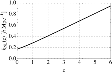
Appendix B Assumptions about the cm signal
The cm brightness temperature is assumed to be
| (14) |
where the expression in the last bracket approximates the cosmic evolution of . This is consistent with Obuljen et al. (2018) and other recent literature Obuljen et al. (2019); Hu et al. (2019). For derivation of the brightness temperature, see e.g. Battye et al. (2013). We have in addition assumed evolution of cosmic from Crighton et al. (2015).
The total power-spectrum signal observed by the radio interferometer is approximately given by
| (15) |
where the first term is the large-scale power spectrum modeled using linear biasing and redshift-space distortions, is the shot-noise contribution from halos making up the neutral hydrogen signal (and usually irrelevant) and is the noise coming from the finite system temperature of the instrument (see App. D).
For the neutral hydrogen large-scale bias and shot-noise, we used results from Castorina and Villaescusa-Navarro (2017) at redshifts beyond , interpolating to results from the Illustris simulation Villaescusa-Navarro et al. (2018). Using the Illustris simulation helps in understanding (and, in future, constraining) the details of the physics ingredients that lead to the observed HI abundances and clustering, and also enables comparison with halo model tools. While the Illustris TNG is also likely to be an imperfect description, it is the best simulation we currently have. Shot-noise is also highly uncertain, but is also very sub-dominant and does not significantly affect results. This interpolation is illustrated in the Figure 33.
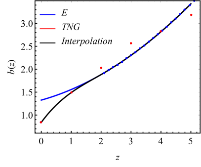 |
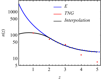 |
At the high redshifts considered here, the linear bias assumption should be a decent approximation down to considerably smaller scales than for galaxies at lower redshift. Following Font-Ribera et al. (2014), we assume an effective maximum wave-number . The idea is that in practice one will fit the data to somewhat larger , which would allow one to constrain and marginalise beyond-linear order bias parameters. We assume a Planck 2015 best-fit cosmology, an assumption that should not affect the results in any significant way.
Appendix C Foreground filtering and foreground wedge considerations
Foregrounds present a major calibration issue for cm cosmology. At a minimum, one loses low modes due to filtering of smooth foregrounds. Many foregrounds on the sky are (within a crude approximation) slowly varying functions of frequency de Oliveira-Costa et al. (2008); Adam et al. (2016); Jelić et al. (2008), so a perfectly calibrated instrument will have a minimum accessible (i.e., not foreground contaminated) value of corresponding to the fundamental mode that fits in the radial range under consideration. In practice, however, amplifier gain stability and beam response changes due to changing environmental factors (e.g. temperature affecting the shape of the reflector), mean that the lowest accessible will be somewhat higher. It is useful to parameterize this in terms of the fractional bandwidth over which we consider the instrument can be perfectly calibrated, since both mechanical and analog electronic drivers scale with . In Figure 34 we plot the minimum value of (and thus total ) accessible as a function of fractional bandwidth. We find that it is only a weak function of redshift. For 20% fractional bandwidth we find that is appropriate over a wide range of redshifts. We shall assume this in our forecasts.
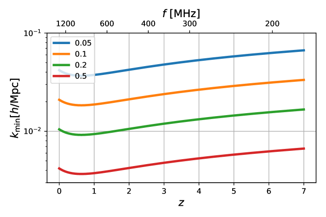
A different issue, first discovered in the context of the epoch of reionization experiments is the the foreground wedge Datta et al. (2010); Vedantham et al. (2012); Morales et al. (2012); Parsons et al. (2012); Trott et al. (2012); Thyagarajan et al. (2013); Pober et al. (2013); Dillon et al. (2014); Hazelton et al. (2013); Thyagarajan et al. (2015a, b); Liu et al. (2014a, b); Pober (2015); Chapman et al. (2016); Pober et al. (2016); Seo and Hirata (2016); Jensen et al. (2016); Kohn et al. (2016) (see also Section 1.5). It has mainly been studied for interferometric cm experiments, although a related issue also exists for single-dish experiments. The foreground wedge results from the fact that a given interferometric baseline has a fixed physical length, which implies that it probes different angular scales at different frequencies (). Interferometers are therefore inherently chromatic, and intrinsically smooth-spectrum foregrounds can appear to have significantly more complicated spectra. This effect can be reduced by careful inter-baseline calibration, which could in principle be achieved by a carefully designed array with a sufficient density of baselines. Achieving such calibration requirements in existing experiments, however, has proven elusive.
We model the ‘wedge’ as a cut on , the cosine of the angle along the line of sight, assuming all signal modes with are lost. The wedge is particularly acute at higher redshifts, since the value of increases with redshift (Eq. 16). In general, the wedge effects can be thought of as being caused by sources from different parts of the sky, with sources away from phase center being particularly affected. The most pessimistic case (known as the “horizon wedge”) assumes all sources above the horizon can contaminate the signal. We take a less pessimistic assumption, and only consider contamination from sources that are no further than times the size of the primary beam away from the beam center. In Figure 6, we show the effective loss of observed volume and number of linear modes for these cases for an experiment with 6-m dishes. We see that the effect is dramatic for the horizon wedge, but even in this case our fiducial experiment achieves a fifty-fold increase in the number of measured linear modes compared to an optical survey at .
We take the position that this systematic will have to be overcome to fully exploit the possibilities offered by the cm technique. We reiterate that it is a technical rather than fundamental problem. Instrumental design choices are vital to support this – for example, dishes result in a characteristic ‘pitchfork’-shaped region of foreground contamination within the wedge, which leaves modes between the pure radial () and horizon boundary of the wedge relatively uncontaminated, while dipoles have strong contamination throughout the entire wedge region in Fourier space (i.e., it results in the loss of all modes with ). Other design choices, such as reducing sidelobes and generally improving the stability of the primary beam response with frequency will also be valuable for allowing modes inside the wedge to be recovered. There have also been promising methodological advances that render full wedge calibration realistic in the future Ghosh et al. (2018). Therefore, when forecasting, we use two possibilities: we either assume that the wedge has been completely calibrated out (optimistic) or that calibration allows us to cut at times the position of the primary beam (pessimistic). This is motivated by the notion that for a typical antenna design, the beam response is suppressed at the signal/foreground level at those distances.
The primary-beam wedge assumption was realised by only considering modes that satisfy
| (16) |
where is the maximum angle at which fringes from a monochromatic point source can enter the measurement and be confused with a non-monochromatic source at phase center. Given that the beam shape is idealised in our experiment, we take 161616We note that the factor of 2 in the denominator here is ad-hoc, for an airy disk, the first null as measured from the center is at and we then take this distance to represent an effective full width., although other choices can be found in the literature, e.g. Pober et al. (2014). See next section for the discussion of the effective dish size.
Appendix D Instrumental noise of Stage ii experiment
We take the Stage ii to be a compact square array of fully illuminated dishes with diameter . We assume an integration time of 5 years (at 100% efficiency) over half the sky ().
We take the total system temperature to be
| (17) |
with the following contributions:
-
•
We assume the amplifier noise temperature to be , which is conservative compared to the best available amplifiers (which already reach better noise figures). However, the ultra-wide-band feeds considered in this experiment will pose their own set of challenges. In particular, due to compromises necessary to achieve sufficient coupling to vacuum, the optical efficiency is reduced from unity and is expected to be . A somewhat subtle point is that this optical efficiency factor decreases both signal and the sky noise by the same factor, and as such, we model it by increasing just the effective amplifier noise.
-
•
We expect that a non-negligible fraction of our our primary beam hits the ground at K instead of being coupled to the sky.
-
•
We take the sky temperature to be
(18) This approximation is consistent with assumptions made in the SKA forecasting exercise Bacon et al. (prep); Braun et al. (2017) and also with effective temperature derived by averaging over the Haslam 408 MHz galaxy map Remazeilles et al. (2015) (i.e. approximately taking into account the inverse variance weighting one might do in practice).
These forecasts can be compared to achieved system temperatures. For example, BMX prototype at BNL has an achieved system temperature at 1300MHz of around 70K which compares well to prediction of 80K assuming , and which are more aggressive numbers than what we assume for Stage ii. Similarly, CHIME has achieved a system temperature without sky contribution of around 60K, which is also somewhat better than these equations predict.
The non-uniform illumination of the primary reduces the effective size of the dish. One might naively expect that the dish illumination will further decrease with frequency at fixed physical OMT size. However, practical modelling has shown that this is not the case, as the portion of the total device that is active decreases with frequency, making the beam hitting the primary reflector nearly frequency-independent. We thus assume that the effective dish area is just a scaled version of the physical dish area with aperture efficiency factor of (see Chapter 9.6 of Stutzman and Thiele (2012) for discussion of practically achievable aperture efficiencies), namely
| (19) |
The power spectrum of system noise is then given by (e.g. Obuljen et al. (2018))
| (20) |
where is the comoving distance to the observed slice, cm is the transition rest-frame frequency, is the observing wavelength, is the total survey area, is the number of polarizations per feed, and is the number density of baselines in the plane. The effective collecting area per feed and effective field of view are given by
| (21) |
Many results in the literature rely on the approximation that the baseline density is independent of up to some maximum baseline length : that is, for a square array with receivers,
| (22) |
We have found that this is a surprisingly poor approximation (see Figure 35, also discussed below). Instead, we use the following fitting formula for the number of baselines as a function of physical distance of antennas
| (23) |
where , , and the -plane density is
| (24) |
This formula has been fitted to our fiducial case and calibrated so that . The fitting parameters are
| square close-packing: | |||
| hexagonal close-packing in a compact circle: |
This formula works well down to a very small value of ; even with , the total number of baselines matches the exact calculation to within a few percent. Figure 35 shows the numerical result together with the fitting formula. The shown formula is only true for an observing field at zenith, but we ignore this effect in our forecasting.
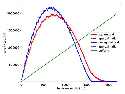
Appendix E Figures 4 and 5
Figures 4 and 5 were made as follows. A numerical simulation with particles in a box of size 300 Mpc/h has been run using the l-picola code (Howlett et al., 2015). Halos were identified using the Friends-of-Friends algorithm (Davis et al., 1985), with a value of the linking length parameter . Neutral hydrogen was then assigned to halos according to Villaescusa-Navarro et al. (2018).
For LSST we assumed a photometric error of and number density according to the fitting formula from the Appendix of Mandelbaum et al. (2018).
For dropout survey we assumed number densities of () and () at and () and () at respectively, following Chen et al. (2019).
For Stage 2 we have assumed foreground filtering of modes with /Mpc, which for the simulation size of this box filters just modes with and . For beam filtering we have applied a simple Gaussian filtering with variance given by the linear size of the array.
References
- Bandura et al. (2019) K. Bandura, E. Castorina, L. Connor, S. Foreman, D. Green, D. Karagiannis, A. Liu, K. W. Masui, D. Meerburg, M. Münchmeyer, L. B. Newburgh, C. Ng, P. O’Connor, A. Obuljen, H. Padmanabhan, B. Saliwanchik, J. R. Shaw, C. Sheehy, P. Stankus, A. Slosar, A. Stebbins, P. T. Timbie, W. Tyndall, F. Villaescusa-Navarro, B. Wallisch, and M. White, “Packed Ultra-wideband Mapping Array (PUMA): A Radio Telescope for Cosmology and Transients,” arXiv e-prints , arXiv:1907.12559 (2019), arXiv:1907.12559 [astro-ph.IM] .
- Dodelson et al. (2016a) S. Dodelson, K. Heitmann, C. Hirata, K. Honscheid, A. Roodman, U. Seljak, A. Slosar, and M. Trodden, “Cosmic Visions Dark Energy: Science,” (2016a), arXiv:1604.07626 [astro-ph.CO] .
- Dodelson et al. (2016b) S. Dodelson, K. Heitmann, C. Hirata, K. Honscheid, A. Roodman, U. Seljak, A. Slosar, and M. Trodden, “Cosmic Visions Dark Energy: Technology,” (2016b), arXiv:1604.07821 [astro-ph.IM] .
- Dawson et al. (2018) K. Dawson, J. Frieman, K. Heitmann, B. Jain, S. Kahn, R. Mandelbaum, S. Perlmutter, and A. Slosar, “Cosmic Visions Dark Energy: Small Projects Portfolio,” (2018), arXiv:1802.07216 [astro-ph.CO] .
- Aghamousa et al. (2016) A. Aghamousa et al. (DESI Collaboration), “The DESI Experiment Part I: Science, Targeting, and Survey Design,” (2016), arXiv:1611.00036 [astro-ph.IM] .
- Abell et al. (2009) P. A. Abell et al. (LSST Science Collaboration), “LSST Science Book, Version 2.0,” (2009), arXiv:0912.0201 [astro-ph.IM] .
- Peterson et al. (2006) J. B. Peterson, K. Bandura, and U. L. Pen, “The Hubble Sphere Hydrogen Survey,” (2006), astro-ph/0606104 [astro-ph] .
- Castorina and White (2019) E. Castorina and M. White, “Measuring the growth of structure with intensity mapping surveys,” JCAP 06, 025 (2019), arXiv:1902.07147 [astro-ph.CO] .
- Modi et al. (2019a) C. Modi, E. Castorina, Y. Feng, and M. White, “Intensity mapping with neutral hydrogen and the Hidden Valley simulations,” (2019a), arXiv:1904.11923 [astro-ph.CO] .
- Chang et al. (2010) T.-C. Chang, U.-L. Pen, K. Bandura, and J. B. Peterson, “An intensity map of hydrogen 21-cm emission at redshift ,” Nature 466, 463 (2010), arXiv:1007.3709 [astro-ph.CO] .
- Davis et al. (2001) M. Davis, J. A. Newman, S. M. Faber, and A. C. Phillips, “The DEEP2 Redshift Survey,” in Deep Fields, edited by S. Cristiani, A. Renzini, and R. E. Williams (2001) p. 241, astro-ph/0012189 [astro-ph] .
- Masui et al. (2013) K. W. Masui et al., “Measurement of 21 cm Brightness Fluctuations at in Cross-correlation,” ApJ 763, L20 (2013), arXiv:1208.0331 [astro-ph.CO] .
- Drinkwater et al. (2010) M. J. Drinkwater et al., “The WiggleZ Dark Energy Survey: Survey Design and First Data Release,” MNRAS 401, 1429 (2010), arXiv:0911.4246 [astro-ph.CO] .
- Switzer et al. (2013) E. R. Switzer et al., “Determination of neutral hydrogen fluctuations using the 21 cm intensity mapping autocorrelation,” MNRAS 434, L46 (2013), arXiv:1304.3712 [astro-ph.CO] .
- Boyle (2018) P. C. Boyle, “First detection of fast radio bursts between 400 and 800 MHz by CHIME/FRB,” The Astronomer’s Telegram 11901 (2018).
- Villaescusa-Navarro et al. (2017) F. Villaescusa-Navarro, D. Alonso, and M. Viel, “Baryonic acoustic oscillations from 21 cm intensity mapping: the Square Kilometre Array case,” MNRAS 466, 2736 (2017), arXiv:1609.00019 [astro-ph.CO] .
- Bull (2016) P. Bull, “Extending Cosmological Tests of General Relativity with the Square Kilometre Array,” ApJ 817, 26 (2016), arXiv:1509.07562 [astro-ph.CO] .
- Parsons et al. (2012) A. R. Parsons, J. C. Pober, J. E. Aguirre, C. L. Carilli, D. C. Jacobs, and D. F. Moore, “A Per-baseline, Delay-spectrum Technique for Accessing the 21 cm Cosmic Reionization Signature,” ApJ 756, 165 (2012), arXiv:1204.4749 [astro-ph.IM] .
- Liu et al. (2014a) A. Liu, A. R. Parsons, and C. M. Trott, “Epoch of reionization window. I. Mathematical formalism,” Phys. Rev. D 90, 023018 (2014a), arXiv:1404.2596 [astro-ph.CO] .
- Liu et al. (2014b) A. Liu, A. R. Parsons, and C. M. Trott, “Epoch of reionization window. II. Statistical methods for foreground wedge reduction,” Phys. Rev. D 90, 023019 (2014b), arXiv:1404.4372 [astro-ph.CO] .
- Ghosh et al. (2018) A. Ghosh, F. Mertens, and L. V. E. Koopmans, “Deconvolving the Wedge: Maximum-Likelihood Power Spectra via Spherical-Wave Visibility Modeling,” MNRAS 474, 4552 (2018), arXiv:1709.06752 [astro-ph.CO] .
- Chen et al. (2019) S.-F. Chen, E. Castorina, M. White, and A. Slosar, “Synergies between radio, optical and microwave observations at high redshift,” JCAP 07, 023 (2019), arXiv:1810.00911 [astro-ph.CO] .
- Vanderlinde (2019) K. Vanderlinde, Private Communication (2019).
- Castorina and Villaescusa-Navarro (2017) E. Castorina and F. Villaescusa-Navarro, “On the spatial distribution of neutral hydrogen in the Universe: bias and shot-noise of the H I power spectrum,” MNRAS 471, 1788 (2017), arXiv:1609.05157 [astro-ph.CO] .
- Villaescusa-Navarro et al. (2018) F. Villaescusa-Navarro et al., “Ingredients for 21 cm Intensity Mapping,” ApJ 866, 135 (2018), arXiv:1804.09180 [astro-ph.CO] .
- Stark et al. (2015a) C. W. Stark, M. White, K.-G. Lee, and J. F. Hennawi, “Protocluster discovery in tomographic Ly forest flux maps,” MNRAS 453, 311 (2015a), arXiv:1412.1507 [astro-ph.CO] .
- Stark et al. (2015b) C. W. Stark, A. Font-Ribera, M. White, and K.-G. Lee, “Finding high-redshift voids using Lyman- forest tomography,” MNRAS 453, 4311 (2015b), arXiv:1504.03290 [astro-ph.CO] .
- Harikane et al. (2018) Y. Harikane et al., “GOLDRUSH. II. Clustering of Galaxies at Revealed with the Half-Million Dropouts Over the 100 deg2 Area Corresponding to 1 Gpc3,” PASJ 70, S11 (2018), arXiv:1704.06535 [astro-ph.GA] .
- Jain and Khoury (2010) B. Jain and J. Khoury, “Cosmological Tests of Gravity,” Ann. Phys. 325, 1479 (2010), arXiv:1004.3294 [astro-ph.CO] .
- Clifton et al. (2012) T. Clifton, P. G. Ferreira, A. Padilla, and C. Skordis, “Modified Gravity and Cosmology,” Phys. Rept. 513, 1 (2012), arXiv:1106.2476 [astro-ph.CO] .
- Weinberg et al. (2013) D. H. Weinberg, M. J. Mortonson, D. J. Eisenstein, C. Hirata, A. G. Riess, and E. Rozo, “Observational Probes of Cosmic Acceleration,” Phys. Rep. 530, 87 (2013), arXiv:1201.2434 [astro-ph.CO] .
- Joyce et al. (2015) A. Joyce, B. Jain, J. Khoury, and M. Trodden, “Beyond the cosmological standard model,” Phys. Rep. 568, 1 (2015), arXiv:1407.0059 [astro-ph.CO] .
- Joyce et al. (2016) A. Joyce, L. Lombriser, and F. Schmidt, “Dark Energy Versus Modified Gravity,” Annu. Rev. Nucl. Part. S. 66, 95 (2016), arXiv:1601.06133 [astro-ph.CO] .
- Amendola et al. (2018) L. Amendola et al., “Cosmology and fundamental physics with the Euclid satellite,” Living Rev. Rel. 21, 2 (2018), arXiv:1606.00180 [astro-ph.CO] .
- Amendola et al. (2013a) L. Amendola et al., “Cosmology and Fundamental Physics with the Euclid Satellite,” Living Rev. Rel. 16, 6 (2013a), arXiv:1206.1225 [astro-ph.CO] .
- Jain et al. (2013) B. Jain et al., “Novel Probes of Gravity and Dark Energy,” (2013), arXiv:1309.5389 [astro-ph.CO] .
- Amendola et al. (2013b) L. Amendola, M. Kunz, M. Motta, I. D. Saltas, and I. Sawicki, “Observables and unobservables in dark energy cosmologies,” Phys. Rev. D 87, 023501 (2013b), arXiv:1210.0439 [astro-ph.CO] .
- Baker et al. (2014a) T. Baker, P. G. Ferreira, C. D. Leonard, and M. Motta, “New Gravitational Scales in Cosmological Surveys,” Phys. Rev. D 90, 124030 (2014a), arXiv:1409.8284 [astro-ph.CO] .
- Leonard et al. (2015) C. D. Leonard, T. Baker, and P. G. Ferreira, “Exploring degeneracies in modified gravity with weak lensing,” Phys. Rev. D 91, 083504 (2015), arXiv:1501.03509 [astro-ph.CO] .
- Khoury and Weltman (2004) J. Khoury and A. Weltman, “Chameleon cosmology,” Phys. Rev. D 69, 044026 (2004), arXiv:astro-ph/0309411 [astro-ph] .
- Hinterbichler and Khoury (2010) K. Hinterbichler and J. Khoury, “Screening Long-Range Forces through Local Symmetry Restoration,” Phys. Rev. Lett. 104, 231301 (2010), arXiv:1001.4525 [hep-th] .
- Brax et al. (2012) P. Brax, A.-C. Davis, B. Li, and H. A. Winther, “Unified description of screened modified gravity,” Phys. Rev. D 86, 044015 (2012), arXiv:1203.4812 [astro-ph.CO] .
- Koyama (2016) K. Koyama, “Cosmological tests of modified gravity,” Rep. Prog. Phys. 79, 046902 (2016), arXiv:1504.04623 [astro-ph.CO] .
- Baker et al. (2015) T. Baker, D. Psaltis, and C. Skordis, “Linking Tests of Gravity on All Scales: from the Strong-field Regime to Cosmology,” ApJ 802, 63 (2015), arXiv:1412.3455 [astro-ph.CO] .
- Berti et al. (2015) E. Berti et al., “Testing general relativity with present and future astrophysical observations,” Class. Quantum Gravity 32, 243001 (2015), arXiv:1501.07274 [gr-qc] .
- Gubitosi et al. (2013) G. Gubitosi, F. Piazza, and F. Vernizzi, “The effective field theory of dark energy,” JCAP 02, 032 (2013), arXiv:1210.0201 [hep-th] .
- Bloomfield et al. (2013) J. Bloomfield, E. E. Flanagan, M. Park, and S. Watson, “Dark energy or modified gravity? An effective field theory approach,” JCAP 08, 010 (2013), arXiv:1211.7054 [astro-ph.CO] .
- Bellini and Sawicki (2014) E. Bellini and I. Sawicki, “Maximal freedom at minimum cost: linear large-scale structure in general modifications of gravity,” JCAP 07, 050 (2014), arXiv:1404.3713 [astro-ph.CO] .
- Abbott et al. (2017) B. P. Abbott et al. (LIGO Scientific, Virgo, Fermi-GBM and INTEGRAL Collaboration), “Gravitational Waves and Gamma-Rays from a Binary Neutron Star Merger: GW170817 and GRB 170817A,” ApJ 848, L13 (2017), arXiv:1710.05834 [astro-ph.HE] .
- Lombriser and Taylor (2016) L. Lombriser and A. Taylor, “Breaking a Dark Degeneracy with Gravitational Waves,” JCAP 03, 031 (2016), arXiv:1509.08458 [astro-ph.CO] .
- Creminelli and Vernizzi (2017) P. Creminelli and F. Vernizzi, “Dark Energy after GW170817 and GRB170817A,” Phys. Rev. Lett. 119, 251302 (2017), arXiv:1710.05877 [astro-ph.CO] .
- Sakstein and Jain (2017) J. Sakstein and B. Jain, “Implications of the Neutron Star Merger GW170817 for Cosmological Scalar-Tensor Theories,” Phys. Rev. Lett. 119, 251303 (2017), arXiv:1710.05893 [astro-ph.CO] .
- Ezquiaga and Zumalacárregui (2017) J. M. Ezquiaga and M. Zumalacárregui, “Dark Energy After GW170817: Dead Ends and the Road Ahead,” Phys. Rev. Lett. 119, 251304 (2017), arXiv:1710.05901 [astro-ph.CO] .
- Baker et al. (2017) T. Baker, E. Bellini, P. G. Ferreira, M. Lagos, J. Noller, and I. Sawicki, “Strong Constraints on Cosmological Gravity from GW170817 and GRB 170817A,” Phys. Rev. Lett. 119, 251301 (2017), arXiv:1710.06394 [astro-ph.CO] .
- Amendola et al. (2018) L. Amendola, M. Kunz, I. D. Saltas, and I. Sawicki, “Fate of Large-Scale Structure in Modified Gravity After GW170817 and GRB170817A,” Phys. Rev. Lett. 120, 131101 (2018), arXiv:1711.04825 [astro-ph.CO] .
- de Rham and Melville (2018) C. de Rham and S. Melville, “Gravitational Rainbows: LIGO and Dark Energy at its Cutoff,” Phys. Rev. Lett. 121, 221101 (2018), arXiv:1806.09417 [hep-th] .
- Raveri et al. (2017) M. Raveri, P. Bull, A. Silvestri, and L. Pogosian, “Priors on the effective dark energy equation of state in scalar-tensor theories,” Phys. Rev. D 96, 083509 (2017), arXiv:1703.05297 [astro-ph.CO] .
- Linder (2006a) E. V. Linder, “Paths of quintessence,” Phys. Rev. D 73, 063010 (2006a), astro-ph/0601052 [astro-ph] .
- di Porto and Amendola (2008) C. di Porto and L. Amendola, “Observational constraints on the linear fluctuation growth rate,” Phys. Rev. D 77, 083508 (2008), arXiv:0707.2686 [astro-ph] .
- Simpson and Peacock (2010) F. Simpson and J. A. Peacock, “Difficulties distinguishing dark energy from modified gravity via redshift distortions,” Phys. Rev. D 81, 043512 (2010), arXiv:0910.3834 [astro-ph.CO] .
- Baker et al. (2014b) T. Baker, P. Ferreira, and C. Skordis, “A fast route to modified gravitational growth,” Phys. Rev. D 89, 024026 (2014b), arXiv:1310.1086 [astro-ph.CO] .
- Perenon et al. (2015) L. Perenon, F. Piazza, C. Marinoni, and L. Hui, “Phenomenology of dark energy: general features of large-scale perturbations,” JCAP 11, 029 (2015), arXiv:1506.03047 [astro-ph.CO] .
- Leo et al. (2019) M. Leo, C. Arnold, and B. Li, “A high-redshift test of gravity using enhanced growth of small structures probed by the neutral hydrogen distribution,” (2019), arXiv:1907.02981 [astro-ph.CO] .
- Percival (2017) W. Percival, “Baryon acoustic oscillations: A cosmological ruler,” Physics Today 70, 32 (2017).
- Tanabashi et al. (2018) M. Tanabashi et al. (Particle Data Group), “Review of Particle Physics,” Phys. Rev. D 98, 030001 (2018).
- Font-Ribera et al. (2014) A. Font-Ribera, P. McDonald, N. Mostek, B. A. Reid, H.-J. Seo, and A. Slosar, “DESI and other Dark Energy experiments in the era of neutrino mass measurements,” JCAP 05, 023 (2014), arXiv:1308.4164 [astro-ph.CO] .
- Obuljen et al. (2018) A. Obuljen, E. Castorina, F. Villaescusa-Navarro, and M. Viel, “High-redshift post-reionisation cosmology with 21cm intensity mapping,” JCAP 05, 004 (2018), arXiv:1709.07893 [astro-ph.CO] .
- Aubourg et al. (2015) E. Aubourg et al. (BOSS Collaboration), “Cosmological implications of baryon acoustic oscillation measurements,” Phys. Rev. D 92, 123516 (2015), arXiv:1411.1074 [astro-ph.CO] .
- Alam et al. (2017) S. Alam et al. (BOSS Collaboration), “The clustering of galaxies in the completed SDSS-III Baryon Oscillation Spectroscopic Survey: cosmological analysis of the DR12 galaxy sample,” MNRAS 470, 2617 (2017), arXiv:1607.03155 [astro-ph.CO] .
- du Mas des Bourboux et al. (2017) H. du Mas des Bourboux et al., “Baryon acoustic oscillations from the complete SDSS-III Ly-quasar cross-correlation function at z = 2.4,” A&A 608, A130 (2017), arXiv:1708.02225 [astro-ph.CO] .
- Slosar et al. (2013) A. Slosar et al., “Measurement of baryon acoustic oscillations in the Lyman- forest fluctuations in BOSS data release 9,” JCAP 04, 026 (2013), arXiv:1301.3459 [astro-ph.CO] .
- Ata et al. (2018) M. Ata et al., “The clustering of the SDSS-IV extended Baryon Oscillation Spectroscopic Survey DR14 quasar sample: first measurement of baryon acoustic oscillations between redshift 0.8 and 2.2,” MNRAS 473, 4773 (2018), arXiv:1705.06373 [astro-ph.CO] .
- Kazin et al. (2014) E. A. Kazin et al., “The WiggleZ Dark Energy Survey: improved distance measurements to with reconstruction of the baryonic acoustic feature,” MNRAS 441, 3524 (2014), arXiv:1401.0358 [astro-ph.CO] .
- Aghanim et al. (2018a) N. Aghanim et al. (Planck Collaboration), “Planck 2018 results. VI. Cosmological parameters,” (2018a), arXiv:1807.06209 [astro-ph.CO] .
- Laureijs et al. (2011) R. Laureijs et al. (Euclid Collaboration), “Euclid Definition Study Report,” (2011), arXiv:1110.3193 [astro-ph.CO] .
- Seo and Eisenstein (2003) H.-J. Seo and D. J. Eisenstein, “Probing Dark Energy with Baryonic Acoustic Oscillations from Future Large Galaxy Redshift Surveys,” ApJ 598, 720 (2003), astro-ph/0307460 [astro-ph] .
- Doran and Robbers (2006) M. Doran and G. Robbers, “Early dark energy cosmologies,” JCAP 06, 026 (2006), astro-ph/0601544 [astro-ph] .
- Karwal and Kamionkowski (2016) T. Karwal and M. Kamionkowski, “Dark energy at early times, the Hubble parameter, and the string axiverse,” Phys. Rev. D 94, 103523 (2016), arXiv:1608.01309 [astro-ph.CO] .
- Bean et al. (2001) R. Bean, S. H. Hansen, and A. Melchiorri, “Early-universe constraints on dark energy,” Phys. Rev. D 64, 103508 (2001), astro-ph/0104162 [astro-ph] .
- Xia and Viel (2009) J.-Q. Xia and M. Viel, “Early dark energy at high redshifts: status and perspectives,” JCAP 04, 002 (2009), arXiv:0901.0605 [astro-ph.CO] .
- Calabrese et al. (2011) E. Calabrese, D. Huterer, E. V. Linder, A. Melchiorri, and L. Pagano, “Limits on dark radiation, early dark energy, and relativistic degrees of freedom,” Phys. Rev. D 83, 123504 (2011), arXiv:1103.4132 [astro-ph.CO] .
- Pettorino et al. (2013) V. Pettorino, L. Amendola, and C. Wetterich, “How early is early dark energy?” Phys. Rev. D 87, 083009 (2013), arXiv:1301.5279 [astro-ph.CO] .
- Linder (2006b) E. V. Linder, “Dark energy in the dark ages,” Astropart. Phys. 26, 16 (2006b), astro-ph/0603584 [astro-ph] .
- Akrami et al. (2018) Y. Akrami et al. (Planck Collaboration), “Planck 2018 results. I. Overview and the cosmological legacy of Planck,” (2018), arXiv:1807.06205 [astro-ph.CO] .
- Crighton et al. (2015) N. H. M. Crighton et al., “The neutral hydrogen cosmological mass density at ,” MNRAS 452, 217 (2015), arXiv:1506.02037 [astro-ph.CO] .
- Padmanabhan et al. (2015) H. Padmanabhan, T. R. Choudhury, and A. Refregier, “Theoretical and observational constraints on the H I intensity power spectrum,” MNRAS 447, 3745 (2015), arXiv:1407.6366 [astro-ph.CO] .
- Rhee et al. (2018) J. Rhee, P. Lah, F. H. Briggs, J. N. Chengalur, M. Colless, S. P. Willner, M. L. N. Ashby, and O. Le Fèvre, “Neutral hydrogen (H I) gas content of galaxies at z 0.32,” MNRAS 473, 1879 (2018), arXiv:1709.07596 [astro-ph.GA] .
- Obuljen et al. (2019) A. Obuljen, D. Alonso, F. Villaescusa-Navarro, I. Yoon, and M. Jones, “The HI content of dark matter halos at from ALFALFA,” MNRAS 486, 5124 (2019), arXiv:1805.00934 [astro-ph.CO] .
- Blake et al. (2012) C. Blake et al., “The WiggleZ Dark Energy Survey: joint measurements of the expansion and growth history at ,” MNRAS 425, 405 (2012), arXiv:1204.3674 [astro-ph.CO] .
- Beutler et al. (2012) F. Beutler et al., “The 6dF Galaxy Survey: zAppl. Phys. 0 measurements of the growth rate and 8,” MNRAS 423, 3430 (2012), arXiv:1204.4725 [astro-ph.CO] .
- Okumura et al. (2016) T. Okumura et al., “The Subaru FMOS galaxy redshift survey (FastSound). IV. New constraint on gravity theory from redshift space distortions at ,” PASJ 68, 38 (2016), arXiv:1511.08083 [astro-ph.CO] .
- Beutler et al. (2017) F. Beutler et al. (BOSS Collaboration), “The clustering of galaxies in the completed SDSS-III Baryon Oscillation Spectroscopic Survey: anisotropic galaxy clustering in Fourier space,” MNRAS 466, 2242 (2017), arXiv:1607.03150 [astro-ph.CO] .
- de la Torre et al. (2017) S. de la Torre et al., “The VIMOS Public Extragalactic Redshift Survey (VIPERS). Gravity test from the combination of redshift-space distortions and galaxy-galaxy lensing at ,” A&A 608, A44 (2017), arXiv:1612.05647 [astro-ph.CO] .
- Zhao et al. (2019) G.-B. Zhao et al., “The clustering of the SDSS-IV extended Baryon Oscillation Spectroscopic Survey DR14 quasar sample: a tomographic measurement of cosmic structure growth and expansion rate based on optimal redshift weights,” MNRAS 482, 3497 (2019), arXiv:1801.03043 [astro-ph.CO] .
- Zumalacárregui et al. (2017) M. Zumalacárregui, E. Bellini, I. Sawicki, J. Lesgourgues, and P. G. Ferreira, “hi_class: Horndeski in the Cosmic Linear Anisotropy Solving System,” JCAP 08, 019 (2017), arXiv:1605.06102 [astro-ph.CO] .
- Blas et al. (2011) D. Blas, J. Lesgourgues, and T. Tram, “The Cosmic Linear Anisotropy Solving System (CLASS). Part II: Approximation schemes,” JCAP 07, 034 (2011), arXiv:1104.2933 [astro-ph.CO] .
- Chluba et al. (2015) J. Chluba, J. Hamann, and S. P. Patil, “Features and New Physical Scales in Primordial Observables: Theory and Observation,” Int. J. Mod. Phys. D24, 1530023 (2015), arXiv:1505.01834 [astro-ph.CO] .
- Slosar et al. (2019a) A. Slosar, X. Chen, C. Dvorkin, D. Green, P. D. Meerburg, E. Silverstein, and B. Wallisch, “Scratches from the Past: Inflationary Archaeology through Features in the Power Spectrum of Primordial Fluctuations,” (2019a), arXiv:1903.09883 [astro-ph.CO] .
- Cyr-Racine et al. (2014) F.-Y. Cyr-Racine, R. de Putter, A. Raccanelli, and K. Sigurdson, “Constraints on Large-Scale Dark Acoustic Oscillations from Cosmology,” Phys. Rev. D 89, 063517 (2014), arXiv:1310.3278 [astro-ph.CO] .
- Flauger et al. (2017) R. Flauger, L. McAllister, E. Silverstein, and A. Westphal, “Drifting Oscillations in Axion Monodromy,” JCAP 10, 055 (2017), arXiv:1412.1814 [hep-th] .
- Achúcarro et al. (2014) A. Achúcarro, V. Atal, P. Ortiz, and J. Torrado, “Localized correlated features in the CMB power spectrum and primordial bispectrum from a transient reduction in the speed of sound,” Phys. Rev. D 89, 103006 (2014), arXiv:1311.2552 [astro-ph.CO] .
- Chen and Namjoo (2014) X. Chen and M. H. Namjoo, “Standard Clock in Primordial Density Perturbations and Cosmic Microwave Background,” Phys. Lett. B739, 285 (2014), arXiv:1404.1536 [astro-ph.CO] .
- Chen et al. (2015) X. Chen, M. H. Namjoo, and Y. Wang, “Models of the Primordial Standard Clock,” JCAP 02, 027 (2015), arXiv:1411.2349 [astro-ph.CO] .
- Meerburg et al. (2012) P. D. Meerburg, R. A. M. J. Wijers, and J. P. van der Schaar, “WMAP7 constraints on oscillations in the primordial power spectrum,” MNRAS 421, 369 (2012), arXiv:1109.5264 [astro-ph.CO] .
- Peiris et al. (2013) H. Peiris, R. Easther, and R. Flauger, “Constraining Monodromy Inflation,” JCAP 09, 018 (2013), arXiv:1303.2616 [astro-ph.CO] .
- Meerburg and Spergel (2014) P. D. Meerburg and D. N. Spergel, “Searching for oscillations in the primordial power spectrum. II. Constraints from Planck data,” Phys. Rev. D 89, 063537 (2014), arXiv:1308.3705 [astro-ph.CO] .
- Easther and Flauger (2014) R. Easther and R. Flauger, “Planck Constraints on Monodromy Inflation,” JCAP 02, 037 (2014), arXiv:1308.3736 [astro-ph.CO] .
- Fergusson et al. (2015) J. Fergusson, H. Gruetjen, E. P. S. Shellard, and B. Wallisch, “Polyspectra Searches for Sharp Oscillatory Features in Cosmic Microwave Sky Data,” Phys. Rev. D 91, 123506 (2015), arXiv:1412.6152 [astro-ph.CO] .
- Ade et al. (2016) P. A. R. Ade et al. (Planck Collaboration), “Planck 2015 results. XX. Constraints on inflation,” Astron. Astrophys. 594, A20 (2016), arXiv:1502.02114 [astro-ph.CO] .
- Akrami et al. (2018) Y. Akrami et al. (Planck Collaboration), “Planck 2018 results. X. Constraints on inflation,” (2018), arXiv:1807.06211 [astro-ph.CO] .
- Beutler et al. (2019) F. Beutler, M. Biagetti, D. Green, A. Slosar, and B. Wallisch, “Primordial Features from Linear to Nonlinear Scales,” (2019), arXiv:1906.08758 [astro-ph.CO] .
- Chen et al. (2016) X. Chen, P. D. Meerburg, and M. Münchmeyer, “The Future of Primordial Features with 21 cm Tomography,” JCAP 09, 023 (2016), arXiv:1605.09364 [astro-ph.CO] .
- Xu et al. (2016) Y. Xu, J. Hamann, and X. Chen, “Precise measurements of inflationary features with 21 cm observations,” Phys. Rev. D 94, 123518 (2016), arXiv:1607.00817 [astro-ph.CO] .
- Baumann et al. (2018a) D. Baumann, D. Green, and B. Wallisch, “Searching for Light Relics with Large-Scale Structure,” JCAP 08, 029 (2018a), arXiv:1712.08067 [astro-ph.CO] .
- Karaçaylı and Padmanabhan (2019) N. G. Karaçaylı and N. Padmanabhan, “Anatomy of Cosmic Tidal Reconstruction,” MNRAS 486, 3864 (2019), arXiv:1904.01387 [astro-ph.CO] .
- Modi et al. (2019b) C. Modi, M. White, A. Slosar, and E. Castorina, “Reconstructing large-scale structure with neutral hydrogen surveys,” (2019b), arXiv:1907.02330 [astro-ph.CO] .
- Chen (2010) X. Chen, “Primordial Non-Gaussianities from Inflation Models,” Adv. Astron. 2010, 638979 (2010), arXiv:1002.1416 [astro-ph.CO] .
- Alvarez et al. (2014) M. Alvarez et al., “Testing Inflation with Large Scale Structure: Connecting Hopes with Reality,” (2014), arXiv:1412.4671 [astro-ph.CO] .
- Meerburg et al. (2019) P. D. Meerburg et al., “Primordial Non-Gaussianity,” (2019), arXiv:1903.04409 [astro-ph.CO] .
- Maldacena (2003) J. M. Maldacena, “Non-Gaussian features of primordial fluctuations in single field inflationary models,” JHEP 05, 013 (2003), arXiv:astro-ph/0210603 [astro-ph] .
- Creminelli and Zaldarriaga (2004) P. Creminelli and M. Zaldarriaga, “Single field consistency relation for the 3-point function,” JCAP 10, 006 (2004), arXiv:astro-ph/0407059 [astro-ph] .
- Komatsu et al. (2009) E. Komatsu et al., “Non-Gaussianity as a Probe of the Physics of the Primordial Universe and the Astrophysics of the Low Redshift Universe,” Astronomy (2009), arXiv:0902.4759 [astro-ph.CO] .
- Chen and Wang (2010) X. Chen and Y. Wang, “Quasi-Single Field Inflation and Non-Gaussianities,” JCAP 04, 027 (2010), arXiv:0911.3380 [hep-th] .
- Baumann and Green (2012) D. Baumann and D. Green, “Signatures of Supersymmetry from the Early Universe,” Phys. Rev. D 85, 103520 (2012), arXiv:1109.0292 [hep-th] .
- Noumi et al. (2013) T. Noumi, M. Yamaguchi, and D. Yokoyama, “Effective field theory approach to quasi-single field inflation and effects of heavy fields,” JHEP 06, 051 (2013), arXiv:1211.1624 [hep-th] .
- Arkani-Hamed and Maldacena (2015) N. Arkani-Hamed and J. Maldacena, “Cosmological Collider Physics,” (2015), arXiv:1503.08043 [hep-th] .
- Lee et al. (2016) H. Lee, D. Baumann, and G. L. Pimentel, “Non-Gaussianity as a Particle Detector,” JHEP 12, 040 (2016), arXiv:1607.03735 [hep-th] .
- Ade et al. (2014) P. A. R. Ade et al. (Planck Collaboration), “Planck 2013 results. XXIV. Constraints on primordial non-Gaussianity,” A&A 571, A24 (2014), arXiv:1303.5084 [astro-ph.CO] .
- Ade et al. (2016) P. A. R. Ade et al. (Planck Collaboration), “Planck 2015 results. XVII. Constraints on primordial non-Gaussianity,” A&A 594, A17 (2016), arXiv:1502.01592 [astro-ph.CO] .
- Abazajian et al. (2016) K. N. Abazajian et al. (CMB-S4 Collaboration), “CMB-S4 Science Book, First Edition,” (2016), arXiv:1610.02743 [astro-ph.CO] .
- Meerburg et al. (2016) P. D. Meerburg, J. Meyers, A. van Engelen, and Y. Ali-Haïmoud, “CMB B-mode non-Gaussianity,” Phys. Rev. D 93, 123511 (2016), arXiv:1603.02243 [astro-ph.CO] .
- Cooray (2006) A. Cooray, “21-cm Background Anisotropies Can Discern Primordial Non-Gaussianity,” Phys. Rev. Lett. 97, 261301 (2006), astro-ph/0610257 [astro-ph] .
- Pillepich et al. (2007) A. Pillepich, C. Porciani, and S. Matarrese, “The Bispectrum of Redshifted 21 Centimeter Fluctuations from the Dark Ages,” Astrophys. J. 662, 1 (2007), arXiv:astro-ph/0611126 [astro-ph] .
- Meerburg et al. (2017) P. D. Meerburg, M. Münchmeyer, J. B. Muñoz, and X. Chen, “Prospects for cosmological collider physics,” JCAP 03, 050 (2017), arXiv:1610.06559 [astro-ph.CO] .
- Lidz et al. (2013) A. Lidz, E. J. Baxter, P. Adshead, and S. Dodelson, “Primordial non-Gaussianity and reionization,” Phys. Rev. D 88, 023534 (2013), arXiv:1304.8049 [astro-ph.CO] .
- Mao et al. (2013) Y. Mao, A. D’Aloisio, J. Zhang, and P. R. Shapiro, “Primordial non-Gaussianity estimation using 21 cm tomography from the epoch of reionization,” Phys. Rev. D 88, 081303 (2013), arXiv:1305.0313 [astro-ph.CO] .
- Crociani et al. (2009) D. Crociani, L. Moscardini, M. Viel, and S. Matarrese, “The effects of primordial non-Gaussianity on the cosmological reionization,” MNRAS 394, 133 (2009), arXiv:0809.3909 [astro-ph] .
- Tashiro and Ho (2013) H. Tashiro and S. Ho, “Constraining primordial non-Gaussianity with CMB-21 cm cross-correlations?” MNRAS 431, 2017 (2013), arXiv:1205.0563 [astro-ph.CO] .
- D’Aloisio et al. (2013) A. D’Aloisio, J. Zhang, P. R. Shapiro, and Y. Mao, “The scale-dependent signature of primordial non-Gaussianity in the large-scale structure of cosmic reionization,” MNRAS 433, 2900 (2013), arXiv:1304.6411 [astro-ph.CO] .
- Camera et al. (2015) S. Camera, M. G. Santos, and R. Maartens, “Probing primordial non-Gaussianity with SKA galaxy redshift surveys: a fully relativistic analysis,” MNRAS 448, 1035 (2015), arXiv:1409.8286 [astro-ph.CO] .
- Li and Ma (2017) Y.-C. Li and Y.-Z. Ma, “Constraints on primordial non-Gaussianity from future Hi intensity mapping experiments,” Phys. Rev. D 96, 063525 (2017), arXiv:1701.00221 [astro-ph.CO] .
- Karagiannis et al. (2018) D. Karagiannis, A. Lazanu, M. Liguori, A. Raccanelli, N. Bartolo, and L. Verde, “Constraining Primordial non-Gaussianity with Bispectrum and Power Spectum from Upcoming Optical and Radio Surveys,” MNRAS 478, 1341 (2018), arXiv:1801.09280 [astro-ph.CO] .
- Creminelli (2003) P. Creminelli, “On non-Gaussianities in single-field inflation,” JCAP 10, 003 (2003), arXiv:astro-ph/0306122 [astro-ph] .
- Baumann et al. (2015) D. Baumann, D. Green, and R. A. Porto, “B-modes and the nature of inflation,” JCAP 01, 016 (2015), arXiv:1407.2621 [hep-th] .
- Baumann et al. (2016) D. Baumann, D. Green, H. Lee, and R. A. Porto, “Signs of analyticity in single-field inflation,” Phys. Rev. D 93, 023523 (2016), arXiv:1502.07304 [hep-th] .
- Aghanim et al. (2018b) N. Aghanim et al. (Planck Collaboration), “Planck 2018 results. VIII. Gravitational lensing,” (2018b), arXiv:1807.06210 [astro-ph.CO] .
- Galitzki et al. (2018) N. Galitzki et al., “The Simons Observatory: Instrument Overview,” Proc. SPIE Int. Soc. Opt. Eng. 10708, 1070804 (2018), arXiv:1808.04493 [astro-ph.IM] .
- Troxel et al. (2018) M. A. Troxel et al. (DES Collaboration), “Dark Energy Survey Year 1 results: Cosmological constraints from cosmic shear,” Phys. Rev. D 98, 043528 (2018), arXiv:1708.01538 [astro-ph.CO] .
- Mandelbaum (2018) R. Mandelbaum, “Weak lensing for precision cosmology,” Ann. Rev. Astron. Astrophys. 56, 393 (2018), arXiv:1710.03235 [astro-ph.CO] .
- Cooray (2004) A. R. Cooray, “Lensing studies with diffuse backgrounds,” New Astron. 9, 173 (2004), arXiv:astro-ph/0309301 [astro-ph] .
- Pen (2004) U.-L. Pen, “Gravitational lensing of epoch-of-reionization gas,” New Astron. 9, 417 (2004), arXiv:astro-ph/0305387 [astro-ph] .
- Zahn and Zaldarriaga (2006) O. Zahn and M. Zaldarriaga, “Lensing reconstruction using redshifted 21cm fluctuations,” Astrophys. J. 653, 922 (2006), arXiv:astro-ph/0511547 [astro-ph] .
- Metcalf and White (2006) R. B. Metcalf and S. D. M. White, “High-resolution imaging of the cosmic mass distribution from gravitational lensing of pregalactic HI,” MNRAS (2006), 10.1111/j.1365-2966.2007.12212.x, arXiv:astro-ph/0611862 [astro-ph] .
- Pourtsidou and Metcalf (2014) A. Pourtsidou and R. B. Metcalf, “Weak lensing with 21cm intensity mapping at ,” MNRAS 439, L36 (2014), arXiv:1311.4484 [astro-ph.CO] .
- Romeo et al. (2018) A. Romeo, R. B. Metcalf, and A. Pourtsidou, “Simulations for 21 cm radiation lensing at EoR redshifts,” MNRAS 474, 1787 (2018), arXiv:1708.01235 [astro-ph.CO] .
- Foreman et al. (2018) S. Foreman, P. D. Meerburg, A. van Engelen, and J. Meyers, “Lensing reconstruction from line intensity maps: the impact of gravitational nonlinearity,” JCAP 07, 046 (2018), arXiv:1803.04975 [astro-ph.CO] .
- Lu and Pen (2008) T. Lu and U.-L. Pen, “Precision of diffuse 21-cm lensing,” MNRAS 388, 1819 (2008), arXiv:0710.1108 [astro-ph] .
- Lu et al. (2010) T. Lu, U.-L. Pen, and O. Dore, “Dark Energy from Large-Scale Structure Lensing Information,” Phys. Rev. D 81, 123015 (2010), arXiv:0905.0499 [astro-ph.CO] .
- Pen et al. (2012) U.-L. Pen, R. Sheth, J. Harnois-Deraps, X. Chen, and Z. Li, “Cosmic Tides,” (2012), arXiv:1202.5804 [astro-ph.CO] .
- Schmidt et al. (2014) F. Schmidt, E. Pajer, and M. Zaldarriaga, “Large-Scale Structure and Gravitational Waves III: Tidal Effects,” Phys. Rev. D 89, 083507 (2014), arXiv:1312.5616 [astro-ph.CO] .
- Zhu et al. (2016) H.-M. Zhu, U.-L. Pen, Y. Yu, X. Er, and X. Chen, “Cosmic tidal reconstruction,” Phys. Rev. D 93, 103504 (2016), arXiv:1511.04680 [astro-ph.CO] .
- Zhu et al. (2018) H.-M. Zhu, U.-L. Pen, Y. Yu, and X. Chen, “Recovering lost 21 cm radial modes via cosmic tidal reconstruction,” Phys. Rev. D 98, 043511 (2018), arXiv:1610.07062 [astro-ph.CO] .
- Alcock and Paczynski (1979) C. Alcock and B. Paczynski, “An evolution free test for non-zero cosmological constant,” Nature 281, 358 (1979).
- Dvorkin et al. (2019) C. Dvorkin et al., “Neutrino Mass from Cosmology: Probing Physics Beyond the Standard Model,” (2019), arXiv:1903.03689 [astro-ph.CO] .
- Lesgourgues et al. (2013) J. Lesgourgues, G. Mangano, G. Miele, and S. Pastor, Neutrino Cosmology (Cambridge University Press, 2013).
- Patterson (2015) R. B. Patterson, “Prospects for Measurement of the Neutrino Mass Hierarchy,” Annu. Rev. Nucl. Part. S. 65, 177 (2015), arXiv:1506.07917 [hep-ex] .
- Archidiacono et al. (2017) M. Archidiacono, T. Brinckmann, J. Lesgourgues, and V. Poulin, “Physical effects involved in the measurements of neutrino masses with future cosmological data,” JCAP 02, 052 (2017), arXiv:1610.09852 [astro-ph.CO] .
- Lattanzi and Gerbino (2018) M. Lattanzi and M. Gerbino, “Status of neutrino properties and future prospects – Cosmological and astrophysical constraints,” Front. Phys. 5, 70 (2018), arXiv:1712.07109 [astro-ph.CO] .
- Green et al. (2019) D. Green et al., “Messengers from the Early Universe: Cosmic Neutrinos and Other Light Relics,” (2019), arXiv:1903.04763 [astro-ph.CO] .
- Baumann et al. (2016) D. Baumann, D. Green, and B. Wallisch, “New Target for Cosmic Axion Searches,” Phys. Rev. Lett. 117, 171301 (2016), arXiv:1604.08614 [astro-ph.CO] .
- Slosar et al. (2019b) A. Slosar et al., “Dark Energy and Modified Gravity,” (2019b), arXiv:1903.12016 [astro-ph.CO] .
- Meyers (2015) J. Meyers, private communication (2015).
- Seljak (2009) U. Seljak, “Extracting Primordial Non-Gaussianity without Cosmic Variance,” Phys. Rev. Lett. 102, 021302 (2009), arXiv:0807.1770 [astro-ph] .
- McDonald and Seljak (2009) P. McDonald and U. Seljak, “How to evade the sample variance limit on measurements of redshift-space distortions,” JCAP 10, 007 (2009), arXiv:0810.0323 [astro-ph] .
- Carucci et al. (2017) I. P. Carucci, F. Villaescusa-Navarro, and M. Viel, “The cross-correlation between 21 cm intensity mapping maps and the Ly forest in the post-reionization era,” JCAP 04, 001 (2017), arXiv:1611.07527 [astro-ph.CO] .
- Hill et al. (2008) G. J. Hill et al., “The Hobby-Eberly Telescope Dark Energy Experiment (HETDEX): Description and Early Pilot Survey Results,” ASP Conf. Ser. 399, 115 (2008), arXiv:0806.0183 [astro-ph] .
- Terrana et al. (2017) A. Terrana, M.-J. Harris, and M. C. Johnson, “Analyzing the cosmic variance limit of remote dipole measurements of the cosmic microwave background using the large-scale kinetic Sunyaev Zel’dovich effect,” JCAP 02, 040 (2017), arXiv:1610.06919 [astro-ph.CO] .
- Deutsch et al. (2018) A.-S. Deutsch, E. Dimastrogiovanni, M. C. Johnson, M. Münchmeyer, and A. Terrana, “Reconstruction of the remote dipole and quadrupole fields from the kinetic Sunyaev Zel’dovich and polarized Sunyaev Zel’dovich effects,” Phys. Rev. D 98, 123501 (2018), arXiv:1707.08129 [astro-ph.CO] .
- Cayuso et al. (2018) J. I. Cayuso, M. C. Johnson, and J. B. Mertens, “Simulated reconstruction of the remote dipole field using the kinetic Sunyaev Zel’dovich effect,” Phys. Rev. D 98, 063502 (2018), arXiv:1806.01290 [astro-ph.CO] .
- Smith et al. (2018) K. M. Smith, M. S. Madhavacheril, M. Münchmeyer, S. Ferraro, U. Giri, and M. C. Johnson, “KSZ tomography and the bispectrum,” (2018), arXiv:1810.13423 [astro-ph.CO] .
- Münchmeyer et al. (2018) M. Münchmeyer, M. S. Madhavacheril, S. Ferraro, M. C. Johnson, and K. M. Smith, “Constraining local non-Gaussianities with kSZ tomography,” (2018), arXiv:1810.13424 [astro-ph.CO] .
- Contreras et al. (2019) D. Contreras, M. C. Johnson, and J. B. Mertens, “Towards detection of relativistic effects in galaxy number counts using kSZ Tomography,” (2019), arXiv:1904.10033 [astro-ph.CO] .
- Pan and Johnson (2019) Z. Pan and M. C. Johnson, “Forecasted constraints on modified gravity from Sunyaev Zel’dovich tomography,” (2019), arXiv:1906.04208 [astro-ph.CO] .
- Madhavacheril et al. (2019) M. S. Madhavacheril, N. Battaglia, K. M. Smith, and J. L. Sievers, “Cosmology with kSZ: breaking the optical depth degeneracy with Fast Radio Bursts,” (2019), arXiv:1901.02418 [astro-ph.CO] .
- Cayuso and Johnson (2019) J. I. Cayuso and M. C. Johnson, “Towards testing CMB anomalies using the kinetic and polarized Sunyaev Zel’dovich effects,” (2019), arXiv:1904.10981 [astro-ph.CO] .
- Zhang and Johnson (2015) P. Zhang and M. C. Johnson, “Testing eternal inflation with the kinetic Sunyaev Zel’dovich effect,” JCAP 06, 046 (2015), arXiv:1501.00511 [astro-ph.CO] .
- Padmanabhan et al. (2019) H. Padmanabhan, A. Refregier, and A. Amara, “Impact of astrophysics on cosmology forecasts for 21 cm surveys,” MNRAS 485, 4060 (2019), arXiv:1804.10627 [astro-ph.CO] .
- Abazajian et al. (2019) K. Abazajian et al., “CMB-S4 Science Case, Reference Design, and Project Plan,” (2019), arXiv:1907.04473 [astro-ph.IM] .
- Kim et al. (2015) A. G. Kim, E. V. Linder, J. Edelstein, and D. Erskine, “Giving cosmic redshift drift a whirl,” Astropart. Phys. 62, 195 (2015), arXiv:1402.6614 [astro-ph.CO] .
- Yu et al. (2014) H.-R. Yu, T.-J. Zhang, and U.-L. Pen, “Method for Direct Measurement of Cosmic Acceleration by 21-cm Absorption Systems,” Phys. Rev. Lett. 113, 041303 (2014), arXiv:1311.2363 [astro-ph.CO] .
- Newburgh et al. (2016) L. B. Newburgh et al., “HIRAX: A Probe of Dark Energy and Radio Transients,” Proc. SPIE Int. Soc. Opt. Eng. 9906, 99065X (2016), arXiv:1607.02059 [astro-ph.IM] .
- Bailes et al. (2017) M. Bailes et al., “The UTMOST: A Hybrid Digital Signal Processor Transforms the Molonglo Observatory Synthesis Telescope,” PASA 34, e045 (2017), arXiv:1708.09619 [astro-ph.IM] .
- Amiri et al. (2018) M. Amiri et al. (CHIME/FRB Collaboration), “The CHIME Fast Radio Burst Project: System Overview,” 863, 48 (2018), arXiv:1803.11235 [astro-ph.IM] .
- Lorimer et al. (2007) D. R. Lorimer, M. Bailes, M. A. McLaughlin, D. J. Narkevic, and F. Crawford, “A Bright Millisecond Radio Burst of Extragalactic Origin,” Science 318, 777 (2007), arXiv:0709.4301 [astro-ph] .
- Thornton et al. (2013) D. Thornton et al., “A Population of Fast Radio Bursts at Cosmological Distances,” Science 341, 53 (2013), arXiv:1307.1628 [astro-ph.HE] .
- Masui et al. (2015) K. Masui et al., “Dense magnetized plasma associated with a fast radio burst,” Nature 528, 523 (2015), arXiv:1512.00529 [astro-ph.HE] .
- Chatterjee et al. (2017) S. Chatterjee et al., “A direct localization of a fast radio burst and its host,” Nature 541, 58 (2017), arXiv:1701.01098 [astro-ph.HE] .
- Tendulkar et al. (2017) S. P. Tendulkar et al., “The Host Galaxy and Redshift of the Repeating Fast Radio Burst FRB 121102,” ApJ 834, L7 (2017), arXiv:1701.01100 [astro-ph.HE] .
- Tanimura et al. (2019) H. Tanimura, G. Hinshaw, I. G. McCarthy, L. Van Waerbeke, Y.-Z. Ma, A. Mead, A. Hojjati, and T. Tröster, “A Search for Warm/Hot Gas Filaments Between Pairs of SDSS Luminous Red Galaxies,” MNRAS 483, 223 (2019), arXiv:1709.05024 [astro-ph.CO] .
- de Graaff et al. (2019) A. de Graaff, Y.-C. Cai, C. Heymans, and J. A. Peacock, “Probing the missing baryons with the Sunyaev-Zel’dovich effect from filaments,” Astron. Astrophys. 624, A48 (2019), arXiv:1709.10378 [astro-ph.CO] .
- McQuinn (2014) M. McQuinn, “Locating the “Missing” Baryons with Extragalactic Dispersion Measure Estimates,” ApJ 780, L33 (2014), arXiv:1309.4451 [astro-ph.CO] .
- Masui and Sigurdson (2015) K. W. Masui and K. Sigurdson, “Dispersion Distance and the Matter Distribution of the Universe in Dispersion Space,” Phys. Rev. Lett. 115, 121301 (2015), arXiv:1506.01704 [astro-ph.CO] .
- Chawla et al. (2017) P. Chawla et al., “A Search for Fast Radio Bursts with the GBNCC Pulsar Survey,” ApJ 844, 140 (2017), arXiv:1701.07457 [astro-ph.HE] .
- Arzoumanian et al. (2018) Z. Arzoumanian et al. (NANOGrav Collaboration), “The NANOGrav 11-year Data Set: High-precision Timing of 45 Millisecond Pulsars,” ApJS 235, 37 (2018), arXiv:1801.01837 [astro-ph.HE] .
- Taylor et al. (2015) S. R. Taylor et al., “Limits on Anisotropy in the Nanohertz Stochastic Gravitational Wave Background,” Phys. Rev. Lett. 115, 041101 (2015), arXiv:1506.08817 [astro-ph.HE] .
- Shannon et al. (2013) R. M. Shannon et al., “Gravitational-wave Limits from Pulsar Timing Constrain Supermassive Black Hole Evolution,” Science 342, 334 (2013), arXiv:1310.4569 [astro-ph.CO] .
- Taylor and Weisberg (1989) J. H. Taylor and J. M. Weisberg, “Further experimental tests of relativistic gravity using the binary pulsar PSR 1913 + 16,” ApJ 345, 434 (1989).
- Kramer et al. (2006) M. Kramer et al., “Tests of General Relativity from Timing the Double Pulsar,” Science 314, 97 (2006), astro-ph/0609417 [astro-ph] .
- Stovall et al. (2014) K. Stovall et al., “The Green Bank Northern Celestial Cap Pulsar Survey. I. Survey Description, Data Analysis, and Initial Results,” ApJ 791, 67 (2014), arXiv:1406.5214 [astro-ph.HE] .
- Smith (2016) K. M. Smith, “New algorithms for radio pulsar search,” (2016), arXiv:1610.06831 [astro-ph.HE] .
- Keane et al. (2015) E. Keane et al., “A Cosmic Census of Radio Pulsars with the SKA,” PoS AASKA14, 40 (2015), arXiv:1501.00056 [astro-ph.IM] .
- Manchester et al. (2005) R. N. Manchester, G. B. Hobbs, A. Teoh, and M. Hobbs, “The Australia Telescope National Facility Pulsar Catalogue,” AJ 129, 1993 (2005), arXiv:astro-ph/0412641 [astro-ph] .
- Bandura et al. (2014) K. Bandura et al., “Canadian Hydrogen Intensity Mapping Experiment (CHIME) pathfinder,” Proc. SPIE Int. Soc. Opt. Eng. 9145, 22 (2014), arXiv:1406.2288 [astro-ph.IM] .
- DeBoer et al. (2017) D. R. DeBoer et al., “Hydrogen Epoch of Reionization Array (HERA),” Publ. Astron. Soc. Pac. 129, 045001 (2017), arXiv:1606.07473 [astro-ph.IM] .
- Pober et al. (2013) J. C. Pober et al., “Opening the 21 cm Epoch of Reionization Window: Measurements of Foreground Isolation with PAPER,” ApJ 768, L36 (2013), arXiv:1301.7099 [astro-ph.CO] .
- Tingay et al. (2012) S. Tingay et al., “Realisation of a low frequency SKA Precursor: The Murchison Widefield Array,” PoS RTS2012, 36 (2012), arXiv:1212.1327 [astro-ph.IM] .
- Chen (2012) X. Chen, “The Tianlai Project: a 21CM Cosmology Experiment,” Int. J. Mod. Phys. Conf. Ser. 12, 256 (2012), arXiv:1212.6278 [astro-ph.IM] .
- van Haarlem et al. (2013) M. P. van Haarlem et al., “LOFAR: The LOw-Frequency ARray,” A&A 556, A2 (2013), arXiv:1305.3550 [astro-ph.IM] .
- Monsalve et al. (2017) R. A. Monsalve, A. E. E. Rogers, J. D. Bowman, and T. J. Mozdzen, “Calibration of the EDGES High-band Receiver to Observe the Global 21 cm Signature from the Epoch of Reionization,” ApJ 835, 49 (2017), arXiv:1602.08065 [astro-ph.IM] .
- Greenhili et al. (2012) L. J. Greenhili, D. Werthimer, G. B. Taylor, and S. W. Ellingson, “A broadband 512-element full correlation imaging array at VHF (LEDA),” in 2012 International Conference on Electromagnetics in Advanced Applications (2012) p. 1117.
- Rawlings et al. (2004) S. Rawlings, F. B. Abdalla, S. L. Bridle, C. A. Blake, C. M. Baugh, L. J. Greenhill, and J. M. van der Hulst, “Galaxy evolution, cosmology and dark energy with the Square Kilometer Array,” New A Rev. 48, 1013 (2004), astro-ph/0409479 [astro-ph] .
- Bandura et al. (2016) K. Bandura, J. F. Cliche, M. A. Dobbs, A. J. Gilbert, D. Ittah, J. Mena Parra, and G. Smecher, “ICE-Based Custom Full-Mesh Network for the CHIME High Bandwidth Radio Astronomy Correlator,” J. Astron. Instrum. 5, 1641004 (2016), arXiv:1608.04347 [astro-ph.IM] .
- Berger et al. (2016) P. Berger et al., “Holographic Beam Mapping of the CHIME Pathfinder Array,” Proc. SPIE Int. Soc. Opt. Eng. 9906, 99060D (2016), arXiv:1607.01473 [astro-ph.IM] .
- Newburgh et al. (2014) L. B. Newburgh et al., “Calibrating CHIME: a new radio interferometer to probe dark energy,” Proc. SPIE Int. Soc. Opt. Eng. 9145, 4V (2014), arXiv:1406.2267 [astro-ph.IM] .
- Procopio et al. (2017) P. Procopio et al., “A High-Resolution Foreground Model for the MWA EoR1 Field: Model and Implications for EoR Power Spectrum Analysis,” PASA 34, e033 (2017), arXiv:1707.02288 [astro-ph.IM] .
- Seo and Hirata (2016) H.-J. Seo and C. M. Hirata, “The foreground wedge and 21-cm BAO surveys,” MNRAS 456, 3142 (2016), arXiv:1508.06503 [astro-ph.CO] .
- Liu and Tegmark (2012) A. Liu and M. Tegmark, “How well can we measure and understand foregrounds with 21-cm experiments?” MNRAS 419, 3491 (2012), arXiv:1106.0007 [astro-ph.CO] .
- Shaw et al. (2015) J. R. Shaw, K. Sigurdson, M. Sitwell, A. Stebbins, and U.-L. Pen, “Coaxing Cosmic 21cm Fluctuations from the Polarized Sky using m-mode Analysis,” Phys. Rev. D 91, 083514 (2015), arXiv:1401.2095 [astro-ph.CO] .
- Shaw et al. (2014) J. R. Shaw, K. Sigurdson, U.-L. Pen, A. Stebbins, and M. Sitwell, “All-Sky Interferometry with Spherical Harmonic Transit Telescopes,” Astrophys. J. 781, 57 (2014), arXiv:1302.0327 [astro-ph.CO] .
- Tegmark and Zaldarriaga (2009) M. Tegmark and M. Zaldarriaga, “Fast Fourier transform telescope,” Phys. Rev. D 79, 083530 (2009), arXiv:0805.4414 [astro-ph] .
- Offringa et al. (2015) A. R. Offringa et al., “The Low-Frequency Environment of the Murchison Widefield Array: Radio-Frequency Interference Analysis and Mitigation,” PASA 32, e008 (2015), arXiv:1501.03946 [astro-ph.IM] .
- Offringa et al. (2012) A. R. Offringa, J. J. van de Gronde, and J. B. T. M. Roerdink, “A morphological algorithm for improving radio-frequency interference detection,” A&A 539, A95 (2012), arXiv:1201.3364 [astro-ph.IM] .
- Arora et al. (2015) B. S. Arora et al., “Ionospheric Modelling using GPS to Calibrate the MWA. I: Comparison of First Order Ionospheric Effects between GPS Models and MWA Observations,” PASA 32, e029 (2015), arXiv:1507.01184 [astro-ph.IM] .
- Hovey et al. (2015) G. Hovey et al., “Dish verification antenna-1: A next generation antenna for cm-wave radio telescopes,” in 2015 1st URSI Atlantic Radio Science Conference (URSI AT-RASC) (2015) p. 1.
- Liu et al. (2010) A. Liu, M. Tegmark, S. Morrison, A. Lutomirski, and M. Zaldarriaga, “Precision calibration of radio interferometers using redundant baselines,” MNRAS 408, 1029 (2010), arXiv:1001.5268 [astro-ph.IM] .
- Carilli et al. (2018) C. L. Carilli et al., “HI 21cm Cosmology and the Bi-spectrum: Closure Diagnostics in Massively Redundant Interferometric Arrays,” Radio Sci. 53, 845 (2018), arXiv:1805.00953 [astro-ph.IM] .
- Dillon et al. (2018) J. S. Dillon et al., “Polarized redundant-baseline calibration for 21 cm cosmology without adding spectral structure,” MNRAS 477, 5670 (2018), arXiv:1712.07212 [astro-ph.IM] .
- Ram Marthi and Chengalur (2014) V. Ram Marthi and J. Chengalur, “Non-linear redundancy calibration,” in Astronomical Society of India Conference Series, Vol. 13 (2014) p. 393, arXiv:1310.1449 [astro-ph.IM] .
- Dillon and Parsons (2016) J. S. Dillon and A. R. Parsons, “Redundant Array Configurations for 21 cm Cosmology,” ApJ 826, 181 (2016), arXiv:1602.06259 [astro-ph.IM] .
- Sievers (2017) J. L. Sievers, “Calibration of Quasi-Redundant Interferometers,” (2017), arXiv:1701.01860 [astro-ph.IM] .
- Tegmark and Zaldarriaga (2010) M. Tegmark and M. Zaldarriaga, “Omniscopes: Large area telescope arrays with only computational cost,” Phys. Rev. D 82, 103501 (2010), arXiv:0909.0001 [astro-ph.CO] .
- Masui et al. (2017) K. W. Masui, J. R. Shaw, C. Ng, K. M. Smith, K. Vanderlinde, and A. Paradise, “Algorithms for FFT Beamforming Radio Interferometers,” (2017), arXiv:1710.08591 [astro-ph.IM] .
- Sokolowski et al. (2017) M. Sokolowski et al., “Calibration and Stokes Imaging with Full Embedded Element Primary Beam Model for the Murchison Widefield Array,” PASA 34, e062 (2017), arXiv:1710.07478 [astro-ph.IM] .
- Jacobs et al. (2016) D. C. Jacobs, J. Burba, J. Bowman, A. R. Neben, B. Stinnett, and L. Turner, “The External Calibrator for Hydrogen Observatories,” (2016), arXiv:1610.02607 [astro-ph.IM] .
- Virone et al. (2014) G. Virone et al., “Antenna Pattern Verification System Based on a Micro Unmanned Aerial Vehicle (UAV),” IEEE Antennas Wirel. Propag. Lett. 13, 169 (2014).
- Pupillo et al. (2015) G. Pupillo et al., “Medicina array demonstrator: calibration and radiation pattern characterization using a UAV-mounted radio-frequency source,” Experimental Astronomy 39, 405 (2015).
- Chang et al. (2015) C. Chang, C. Monstein, A. Refregier, A. Amara, A. Glauser, and S. Casura, “Beam Calibration of Radio Telescopes with Drones,” PASP 127, 1131 (2015), arXiv:1505.05885 [astro-ph.IM] .
- D’Addario and Wang (2016) L. R. D’Addario and D. Wang, “A low-power correlator ASIC for arrays with many antennas,” in 2016 United States National Committee of URSI National Radio Science Meeting (USNC-URSI NRSM) (2016) p. 1.
- Harper and Dickinson (2018) S. E. Harper and C. Dickinson, “Potential impact of global navigation satellite services on total power H I intensity mapping surveys,” MNRAS 479, 2024 (2018), arXiv:1803.06314 [astro-ph.IM] .
- Seo et al. (2010) H.-J. Seo, S. Dodelson, J. Marriner, D. Mcginnis, A. Stebbins, C. Stoughton, and A. Vallinotto, “A Ground-based 21 cm Baryon Acoustic Oscillation Survey,” ApJ 721, 164 (2010), arXiv:0910.5007 [astro-ph.CO] .
- Pober (2015) J. C. Pober, “The impact of foregrounds on redshift space distortion measurements with the highly redshifted 21-cm line,” MNRAS 447, 1705 (2015), arXiv:1411.2050 [astro-ph.CO] .
- Jewell et al. (2004) J. Jewell, S. Levin, and C. H. Anderson, “Application of Monte Carlo Algorithms to the Bayesian Analysis of the Cosmic Microwave Background,” ApJ 609, 1 (2004), arXiv:astro-ph/0209560 [astro-ph] .
- Eisenstein et al. (2007) D. J. Eisenstein, H.-J. Seo, E. Sirko, and D. N. Spergel, “Improving Cosmological Distance Measurements by Reconstruction of the Baryon Acoustic Peak,” ApJ 664, 675 (2007), astro-ph/0604362 [astro-ph] .
- Padmanabhan et al. (2009) N. Padmanabhan, M. White, and J. D. Cohn, “Reconstructing baryon oscillations: A Lagrangian theory perspective,” Phys. Rev. D 79, 063523 (2009), arXiv:0812.2905 [astro-ph] .
- Alonso et al. (2014) D. Alonso, P. G. Ferreira, and M. G. Santos, “Fast simulations for intensity mapping experiments,” MNRAS 444, 3183 (2014), arXiv:1405.1751 [astro-ph.CO] .
- Padmanabhan et al. (2017) H. Padmanabhan, A. Refregier, and A. Amara, “A halo model for cosmological neutral hydrogen : abundances and clustering,” MNRAS 469, 2323 (2017), arXiv:1611.06235 [astro-ph.CO] .
- Padmanabhan and Refregier (2017) H. Padmanabhan and A. Refregier, “Constraining a halo model for cosmological neutral hydrogen,” MNRAS 464, 4008 (2017), arXiv:1607.01021 [astro-ph.CO] .
- Monaco et al. (2013) P. Monaco, E. Sefusatti, S. Borgani, M. Crocce, P. Fosalba, R. K. Sheth, and T. Theuns, “An accurate tool for the fast generation of dark matter halo catalogues,” MNRAS 433, 2389 (2013), arXiv:1305.1505 [astro-ph.CO] .
- Kitaura and Heß (2013) F.-S. Kitaura and S. Heß, “Cosmological structure formation with augmented Lagrangian perturbation theory,” MNRAS 435, L78 (2013), arXiv:1212.3514 [astro-ph.CO] .
- Avila et al. (2015) S. Avila, S. G. Murray, A. Knebe, C. Power, A. S. G. Robotham, and J. Garcia-Bellido, “HALOGEN: a tool for fast generation of mock halo catalogues,” MNRAS 450, 1856 (2015), arXiv:1412.5228 [astro-ph.CO] .
- Chuang et al. (2015) C.-H. Chuang, F.-S. Kitaura, F. Prada, C. Zhao, and G. Yepes, “EZmocks: extending the Zel’dovich approximation to generate mock galaxy catalogues with accurate clustering statistics,” MNRAS 446, 2621 (2015), arXiv:1409.1124 [astro-ph.CO] .
- Vakili et al. (2017) M. Vakili, F.-S. Kitaura, Y. Feng, G. Yepes, C. Zhao, C.-H. Chuang, and C. Hahn, “Accurate halo-galaxy mocks from automatic bias estimation and particle mesh gravity solvers,” MNRAS 472, 4144 (2017), arXiv:1701.03765 [astro-ph.CO] .
- Tassev et al. (2013) S. Tassev, M. Zaldarriaga, and D. J. Eisenstein, “Solving large scale structure in ten easy steps with COLA,” JCAP 06, 036 (2013), arXiv:1301.0322 [astro-ph.CO] .
- White et al. (2014) M. White, J. L. Tinker, and C. K. McBride, “Mock galaxy catalogues using the quick particle mesh method,” MNRAS 437, 2594 (2014), arXiv:1309.5532 [astro-ph.CO] .
- Feng et al. (2016) Y. Feng, M.-Y. Chu, U. Seljak, and P. McDonald, “FASTPM: a new scheme for fast simulations of dark matter and haloes,” MNRAS 463, 2273 (2016), arXiv:1603.00476 [astro-ph.CO] .
- Stein et al. (2019) G. Stein, M. A. Alvarez, and J. R. Bond, “The mass-Peak Patch algorithm for fast generation of deep all-sky dark matter halo catalogues and its N-Body validation,” MNRAS 483, 2236 (2019), arXiv:1810.07727 [astro-ph.CO] .
- Prézeau and Reinecke (2010) G. Prézeau and M. Reinecke, “Algorithm for the Evaluation of Reduced Wigner Matrices,” ApJS 190, 267 (2010), arXiv:1002.1050 [astro-ph.IM] .
- Cianciara et al. (2017) A. J. Cianciara et al., “Simulation and Testing of a Linear Array of Modified Four-Square Feed Antennas for the Tianlai Cylindrical Radio Telescope,” J. Astron. Instrum. 6, 1750003-40 (2017), arXiv:1705.04435 [astro-ph.IM] .
- Deng and Campbell-Wilson (2017) M. Deng and D. Campbell-Wilson, “The cloverleaf antenna: A compact wide-bandwidth dual-polarization feed for CHIME,” (2017), arXiv:1708.08521 [astro-ph.IM] .
- Ewall-Wice et al. (2016) A. Ewall-Wice et al., “The Hydrogen Epoch of Reionization Array Dish. II. Characterization of Spectral Structure with Electromagnetic Simulations and Its Science Implications.” ApJ 831, 196 (2016), arXiv:1602.06277 [astro-ph.CO] .
- (271) “VLA data rate,” https://science.nrao.edu/facilities/vla/docs/manuals/oss/performance/tim-res, accessed: 2018-07-10.
- (272) “ALMA data rate,” https://library.nrao.edu/public/memos/naasc/NAASC_110.pdf, accessed: 2018-07-10.
- (273) “LHC data rate,” https://home.cern/about/computing/processing-what-record, accessed: 2018-07-10.
- (274) “LSST data rate,” https://www.lsst.org/about/camera/features, accessed: 2018-07-10.
- Thayer et al. (2017) J. Thayer et al., “Data systems for the Linac coherent light source,” Adv. Struct. Chem. Imaging 3, 3 (2017).
- (276) “LCLS-II data rate,” http://www.esrf.eu/files/live/sites/www/files/events/conferences/2018/IFDEPS/S8.02.Thayer.pdf, accessed: 2018-07-10.
- (277) “XFEL data rate,” http://www.esrf.eu/files/live/sites/www/files/events/conferences/2018/IFDEPS/S8.01.Kuster.pdf, accessed: 2018-07-10.
- (278) “SKA I data rate,” https://indico.cern.ch/event/184526/contributions/322917/attachments/253364/354189/PAlexander_SKA_Computational_Challenges.pdf, accessed: 2018-07-10.
- (279) “CHIME data rate,” https://chime-experiment.ca/instrument, accessed: 2018-07-10.
- Das et al. (2018) S. Das et al., “Progress in the Construction and Testing of the Tianlai Radio Interferometers,” Proc. SPIE Int. Soc. Opt. Eng. 10708, 1070836 (2018), arXiv:1806.04698 [astro-ph.IM] .
- Parsons et al. (2010) A. R. Parsons et al., “The Precision Array for Probing the Epoch of Reionization: Eight Station Results,” AJ 139, 1468 (2010).
- Tingay et al. (2013) S. J. Tingay et al., “The Murchison Widefield Array: The Square Kilometre Array Precursor at Low Radio Frequencies,” PASA 30, e007 (2013), arXiv:1206.6945 [astro-ph.IM] .
- Paciga et al. (2013) G. Paciga et al., MNRAS 433, 639 (2013), arXiv:1301.5906 [astro-ph.CO] .
- Bowman et al. (2018) J. D. Bowman, A. E. E. Rogers, R. A. Monsalve, T. J. Mozdzen, and N. Mahesh, “An absorption profile centred at 78 megahertz in the sky-averaged spectrum,” Nature 555, 67 (2018), arXiv:1810.05912 [astro-ph.CO] .
- Feng and Holder (2018) C. Feng and G. Holder, “Enhanced global signal of neutral hydrogen due to excess radiation at cosmic dawn,” Astrophys. J. 858, L17 (2018), arXiv:1802.07432 [astro-ph.CO] .
- Hills et al. (2018) R. Hills, G. Kulkarni, P. D. Meerburg, and E. Puchwein, “Concerns about modelling of the EDGES data,” Nature 564, E32 (2018), arXiv:1805.01421 [astro-ph.CO] .
- Fraser et al. (2018) S. Fraser et al., “The EDGES 21 cm Anomaly and Properties of Dark Matter,” Phys. Lett. B 785, 159 (2018), arXiv:1803.03245 [hep-ph] .
- Barkana et al. (2018) R. Barkana, N. J. Outmezguine, D. Redigolo, and T. Volansky, “Strong constraints on light dark matter interpretation of the EDGES signal,” Phys. Rev. D 98, 103005 (2018), arXiv:1803.03091 [hep-ph] .
- Berlin et al. (2018) A. Berlin, D. Hooper, G. Krnjaic, and S. D. McDermott, “Severely Constraining Dark Matter Interpretations of the 21-cm Anomaly,” Phys. Rev. Lett. 121, 011102 (2018), arXiv:1803.02804 [hep-ph] .
- Barkana (2018) R. Barkana, “Possible interaction between baryons and dark-matter particles revealed by the first stars,” Nature 555, 71 (2018), arXiv:1803.06698 [astro-ph.CO] .
- Slatyer and Wu (2018) T. R. Slatyer and C.-L. Wu, “Early-Universe Constraints on Dark Matter-Baryon Scattering and their Implications for a Global 21cm Signal,” Phys. Rev. D 98, 023013 (2018), arXiv:1803.09734 [astro-ph.CO] .
- Hirano and Bromm (2018) S. Hirano and V. Bromm, “Baryon-dark matter scattering and first star formation,” MNRAS 480, L85 (2018), arXiv:1803.10671 [astro-ph.GA] .
- Neufeld et al. (2018) D. A. Neufeld, G. R. Farrar, and C. F. McKee, “Dark Matter that Interacts with Baryons: Density Distribution within the Earth and New Constraints on the Interaction Cross-section,” Astrophys. J. 866, 111 (2018), arXiv:1805.08794 [astro-ph.CO] .
- Yoshiura et al. (2018) S. Yoshiura, K. Takahashi, and T. Takahashi, “Impact of EDGES 21cm Global Signal on Primordial Power Spectrum,” Phys. Rev. D 98, 063529 (2018), arXiv:1805.11806 [astro-ph.CO] .
- Chianese et al. (2019) M. Chianese, P. Di Bari, K. Farrag, and R. Samanta, “Probing relic neutrino decays with 21 cm cosmology,” Phys. Lett. B 790, 64 (2019), arXiv:1805.11717 [hep-ph] .
- Costa et al. (2018) A. A. Costa, R. C. G. Landim, B. Wang, and E. Abdalla, “Interacting Dark Energy: Possible Explanation for 21-cm Absorption at Cosmic Dawn,” Eur. Phys. J. C 78, 746 (2018), arXiv:1803.06944 [astro-ph.CO] .
- Hill and Baxter (2018) J. C. Hill and E. J. Baxter, “Can Early Dark Energy Explain EDGES?” JCAP 08, 037 (2018), arXiv:1803.07555 [astro-ph.CO] .
- Moroi et al. (2018) T. Moroi, K. Nakayama, and Y. Tang, “Axion-Photon Conversion and Effects on 21cm Observation,” Phys. Lett. B 783, 301 (2018), arXiv:1804.10378 [hep-ph] .
- Houston et al. (2018) N. Houston, C. Li, T. Li, Q. Yang, and X. Zhang, “Natural Explanation for 21 cm Absorption Signals via Axion-Induced Cooling,” Phys. Rev. Lett. 121, 111301 (2018), arXiv:1805.04426 [hep-ph] .
- Sikivie (2018) P. Sikivie, “Axion dark matter and the 21-cm signal,” Phys. Dark Univ. , 100289 (2018), arXiv:1805.05577 [astro-ph.CO] .
- Wang and Zhao (2018) Y. Wang and G.-B. Zhao, “Constraining the dark matter-vacuum energy interaction using the EDGES 21-cm absorption signal,” Astrophys. J. 869, 26 (2018), arXiv:1805.11210 [astro-ph.CO] .
- D’Amico et al. (2018) G. D’Amico, P. Panci, and A. Strumia, “Bounds on Dark-Matter Annihilations from 21 cm Data,” Phys. Rev. Lett. 121, 011103 (2018), arXiv:1803.03629 [astro-ph.CO] .
- Yang (2018) Y. Yang, “Contributions of dark matter annihilation to the global 21cm spectrum observed by the EDGES experiment,” Phys. Rev. D 98, 103503 (2018), arXiv:1803.05803 [astro-ph.CO] .
- Cheung et al. (2019) K. Cheung, J.-L. Kuo, K.-W. Ng, and Y.-L. Sming Tsai, “The impact of EDGES 21-cm data on dark matter interactions,” Phys. Lett. B 789, 137 (2019), arXiv:1803.09398 [astro-ph.CO] .
- Clark et al. (2018) S. Clark, B. Dutta, Y. Gao, Y.-Z. Ma, and L. E. Strigari, “21cm Limits on Decaying Dark Matter and Primordial Black Holes,” Phys. Rev. D 98, 043006 (2018), arXiv:1803.09390 [astro-ph.HE] .
- Hektor et al. (2018) A. Hektor, G. Hütsi, L. Marzola, M. Raidal, V. Vaskonen, and H. Veermäe, “Constraining Primordial Black Holes with the EDGES 21-cm Absorption Signal,” Phys. Rev. D 98, 023503 (2018), arXiv:1803.09697 [astro-ph.CO] .
- Lidz and Hui (2018) A. Lidz and L. Hui, “Implications of a Pre-reionization 21 cm Absorption Signal for Fuzzy Dark Matter,” Phys. Rev. D 98, 023011 (2018), arXiv:1805.01253 [astro-ph.CO] .
- Safarzadeh et al. (2018) M. Safarzadeh, E. Scannapieco, and A. Babul, “A limit on the warm dark matter particle mass from the redshifted 21 cm absorption line,” Astrophys. J. 859, L18 (2018), arXiv:1803.08039 [astro-ph.CO] .
- Schneider (2018) A. Schneider, “Constraining Non-Cold Dark Matter Models with the Global 21-cm Signal,” Phys. Rev. D 98, 063021 (2018), arXiv:1805.00021 [astro-ph.CO] .
- Liu et al. (2013) A. Liu, J. R. Pritchard, M. Tegmark, and A. Loeb, “Global 21 cm signal experiments: A designer’s guide,” Phys. Rev. D 87, 043002 (2013), arXiv:1211.3743 [astro-ph.CO] .
- Silk (1968) J. Silk, “Cosmic Black-Body Radiation and Galaxy Formation,” ApJ 151, 459 (1968).
- Ali-Haimoud et al. (2014) Y. Ali-Haimoud, P. D. Meerburg, and S. Yuan, “New light on 21 cm intensity fluctuations from the dark ages,” Phys. Rev. D 89, 083506 (2014), arXiv:1312.4948 [astro-ph.CO] .
- Sigurdson and Furlanetto (2006) K. Sigurdson and S. R. Furlanetto, “Measuring the primordial deuterium abundance during the cosmic dark ages,” Phys. Rev. Lett. 97, 091301 (2006), arXiv:astro-ph/0505173 [astro-ph] .
- Loeb and Zaldarriaga (2004) A. Loeb and M. Zaldarriaga, “Measuring the small-scale power spectrum of cosmic density fluctuations through 21 cm tomography prior to the epoch of structure formation,” Phys. Rev. Lett. 92, 211301 (2004), arXiv:astro-ph/0312134 [astro-ph] .
- Lewis and Challinor (2007) A. Lewis and A. Challinor, “The 21cm angular-power spectrum from the dark ages,” Phys. Rev. D 76, 083005 (2007), arXiv:astro-ph/0702600 [astro-ph] .
- Jester and Falcke (2009) S. Jester and H. Falcke, “Science with a lunar low-frequency array: From the dark ages of the Universe to nearby exoplanets,” New A Rev. 53, 1 (2009), arXiv:0902.0493 [astro-ph.CO] .
- Burns et al. (2017) J. O. Burns et al., “A Space-based Observational Strategy for Characterizing the First Stars and Galaxies Using the Redshifted 21 cm Global Spectrum,” ApJ 844, 33 (2017), arXiv:1704.02651 [astro-ph.IM] .
- Wolt, et al. (2013) M. K. Wolt, et al. (DEX Collaboration), “A White paper for a low-frequency radion interferometer mission to explore the cosmological Dark Ages for the L2, L3, ESA Cosmic Vision program,” (2013) p. 1.
- Adshead et al. (2011) P. Adshead, R. Easther, J. Pritchard, and A. Loeb, “Inflation and the Scale Dependent Spectral Index: Prospects and Strategies,” JCAP 02, 021 (2011), arXiv:1007.3748 [astro-ph.CO] .
- Muñoz et al. (2015) J. B. Muñoz, Y. Ali-Haïmoud, and M. Kamionkowski, “Primordial non-gaussianity from the bispectrum of 21-cm fluctuations in the dark ages,” Phys. Rev. D 92, 083508 (2015), arXiv:1506.04152 [astro-ph.CO] .
- Baumann et al. (2018b) D. Baumann, G. Goon, H. Lee, and G. L. Pimentel, “Partially Massless Fields During Inflation,” JHEP 04, 140 (2018b), arXiv:1712.06624 [hep-th] .
- Guth (1981) A. H. Guth, “Inflationary universe: A possible solution to the horizon and flatness problems,” Phys. Rev. D 23, 347 (1981).
- Cook and Sorbo (2012) J. L. Cook and L. Sorbo, “Particle production during inflation and gravitational waves detectable by ground-based interferometers,” Phys. Rev. D 85, 023534 (2012), arXiv:1109.0022 [astro-ph.CO] .
- Namba et al. (2016) R. Namba, M. Peloso, M. Shiraishi, L. Sorbo, and C. Unal, “Scale-dependent gravitational waves from a rolling axion,” JCAP 01, 041 (2016), arXiv:1509.07521 [astro-ph.CO] .
- Khoury et al. (2001) J. Khoury, B. A. Ovrut, P. J. Steinhardt, and N. Turok, “The Ekpyrotic universe: Colliding branes and the origin of the hot big bang,” Phys. Rev. D 64, 123522 (2001), arXiv:hep-th/0103239 [hep-th] .
- Lyth (1997) D. H. Lyth, “What would we learn by detecting a gravitational wave signal in the cosmic microwave background anisotropy?” Phys. Rev. Lett. 78, 1861 (1997), arXiv:hep-ph/9606387 [hep-ph] .
- Meerburg et al. (2017) P. D. Meerburg, J. Meyers, K. M. Smith, and A. van Engelen, “Reconstructing CMB fluctuations and the mean reionization optical depth,” Phys. Rev. D 95, 123538 (2017), arXiv:1701.06992 [astro-ph.CO] .
- Meerburg et al. (2015) P. D. Meerburg, R. Hložek, B. Hadzhiyska, and J. Meyers, “Multiwavelength constraints on the inflationary consistency relation,” Phys. Rev. D 91, 103505 (2015), arXiv:1502.00302 [astro-ph.CO] .
- Alizadeh and Hirata (2012) E. Alizadeh and C. M. Hirata, “How to detect gravitational waves through the cross correlation of the galaxy distribution with the CMB polarization,” Phys. Rev. D 85, 123540 (2012), arXiv:1201.5374 [astro-ph.CO] .
- Masui and Pen (2010) K. W. Masui and U.-L. Pen, “Primordial Gravity Wave Fossils and Their Use in Testing Inflation,” Phys. Rev. Lett. 105, 161302 (2010), arXiv:1006.4181 [astro-ph.CO] .
- Masui et al. (2017) K. W. Masui, U.-L. Pen, and N. Turok, “Two- and Three-Dimensional Probes of Parity in Primordial Gravity Waves,” Phys. Rev. Lett. 118, 221301 (2017), arXiv:1702.06552 [astro-ph.CO] .
- Dodelson et al. (2003) S. Dodelson, E. Rozo, and A. Stebbins, “Primordial gravity waves and weak lensing,” Phys. Rev. Lett. 91, 021301 (2003), arXiv:astro-ph/0301177 [astro-ph] .
- Li and Cooray (2006) C. Li and A. Cooray, “Weak Lensing of the Cosmic Microwave Background by Foreground Gravitational Waves,” Phys. Rev. D 74, 023521 (2006), arXiv:astro-ph/0604179 [astro-ph] .
- Book et al. (2012) L. Book, M. Kamionkowski, and F. Schmidt, “Lensing of 21-cm Fluctuations by Primordial Gravitational Waves,” Phys. Rev. Lett. 108, 211301 (2012), arXiv:1112.0567 [astro-ph.CO] .
- Chisari et al. (2014) N. E. Chisari, C. Dvorkin, and F. Schmidt, “Can weak lensing surveys confirm BICEP2?” Phys. Rev. D 90, 043527 (2014), arXiv:1406.4871 [astro-ph.CO] .
- Sheere et al. (2017) C. Sheere, A. van Engelen, P. D. Meerburg, and J. Meyers, “Establishing the origin of CMB B-mode polarization,” Phys. Rev. D 96, 063508 (2017), arXiv:1610.09365 [astro-ph.CO] .
- Schmidt and Jeong (2012) F. Schmidt and D. Jeong, “Large-Scale Structure with Gravitational Waves II: Shear,” Phys. Rev. D 86, 083513 (2012), arXiv:1205.1514 [astro-ph.CO] .
- Lewis et al. (2000) A. Lewis, A. Challinor, and A. Lasenby, “Efficient computation of CMB anisotropies in closed FRW models,” Astrophys. J. 538, 473 (2000), arXiv:astro-ph/9911177 [astro-ph] .
- Saga et al. (2015) S. Saga, D. Yamauchi, and K. Ichiki, “Weak lensing induced by second-order vector mode,” Phys. Rev. D 92, 063533 (2015), arXiv:1505.02774 [astro-ph.CO] .
- Saga (2016) S. Saga, “Observable cosmological vector mode in the dark ages,” Phys. Rev. D 94, 063523 (2016), arXiv:1607.03973 [astro-ph.CO] .
- Baumann et al. (2007) D. Baumann, P. J. Steinhardt, K. Takahashi, and K. Ichiki, “Gravitational Wave Spectrum Induced by Primordial Scalar Perturbations,” Phys. Rev. D 76, 084019 (2007), arXiv:hep-th/0703290 [hep-th] .
- Foreman et al. (2016) S. Foreman, H. Perrier, and L. Senatore, “Precision Comparison of the Power Spectrum in the EFTofLSS with Simulations,” JCAP 05, 027 (2016), arXiv:1507.05326 [astro-ph.CO] .
- Ma and Scott (2016) Y.-Z. Ma and D. Scott, “How much cosmological information can be measured?” Phys. Rev. D 93, 083510 (2016), arXiv:1510.08309 [astro-ph.CO] .
- Obuljen et al. (2019) A. Obuljen, D. Alonso, F. Villaescusa-Navarro, I. Yoon, and M. Jones, “The H I content of dark matter haloes at from ALFALFA,” MNRAS 486, 5124 (2019), arXiv:1805.00934 [astro-ph.CO] .
- Hu et al. (2019) W. Hu, L. Hoppmann, L. Staveley-Smith, K. Gereb, T. Oosterloo, R. Morganti, B. Catinella, L. Cortese, C. d. P. Lagos, and M. Meyer, “An accurate low-redshift measurement of the cosmic neutral hydrogen density,” (2019), 10.1093/mnras/stz2038, arXiv:1907.10375 [astro-ph.GA] .
- Battye et al. (2013) R. A. Battye, I. W. A. Browne, C. Dickinson, G. Heron, B. Maffei, and A. Pourtsidou, “H I intensity mapping: a single dish approach,” MNRAS 434, 1239 (2013), arXiv:1209.0343 [astro-ph.CO] .
- de Oliveira-Costa et al. (2008) A. de Oliveira-Costa, M. Tegmark, B. M. Gaensler, J. Jonas, T. L. Landecker, and P. Reich, “A model of diffuse Galactic radio emission from 10 MHz to 100 GHz,” MNRAS 388, 247 (2008), arXiv:0802.1525 [astro-ph] .
- Adam et al. (2016) R. Adam et al. (Planck Collaboration), “Planck 2015 results. X. Diffuse component separation: Foreground maps,” A&A 594, A10 (2016), arXiv:1502.01588 [astro-ph.CO] .
- Jelić et al. (2008) V. Jelić et al., “Foreground simulations for the LOFAR-epoch of reionization experiment,” MNRAS 389, 1319 (2008), arXiv:0804.1130 [astro-ph] .
- Datta et al. (2010) A. Datta, J. D. Bowman, and C. L. Carilli, “Bright Source Subtraction Requirements for Redshifted 21 cm Measurements,” ApJ 724, 526 (2010), arXiv:1005.4071 [astro-ph.CO] .
- Vedantham et al. (2012) H. Vedantham, N. Udaya Shankar, and R. Subrahmanyan, “Imaging the Epoch of Reionization: Limitations from Foreground Confusion and Imaging Algorithms,” ApJ 745, 176 (2012), arXiv:1106.1297 [astro-ph.IM] .
- Morales et al. (2012) M. F. Morales, B. Hazelton, I. Sullivan, and A. Beardsley, “Four Fundamental Foreground Power Spectrum Shapes for 21 cm Cosmology Observations,” ApJ 752, 137 (2012), arXiv:1202.3830 [astro-ph.IM] .
- Trott et al. (2012) C. M. Trott, R. B. Wayth, and S. J. Tingay, “The Impact of Point-source Subtraction Residuals on 21 cm Epoch of Reionization Estimation,” ApJ 757, 101 (2012), arXiv:1208.0646 [astro-ph.CO] .
- Thyagarajan et al. (2013) N. Thyagarajan et al., “A Study of Fundamental Limitations to Statistical Detection of Redshifted H I from the Epoch of Reionization,” ApJ 776, 6 (2013), arXiv:1308.0565 [astro-ph.CO] .
- Dillon et al. (2014) J. S. Dillon et al., “Overcoming real-world obstacles in 21 cm power spectrum estimation: A method demonstration and results from early Murchison Widefield Array data,” Phys. Rev. D 89, 023002 (2014), arXiv:1304.4229 [astro-ph.CO] .
- Hazelton et al. (2013) B. J. Hazelton, M. F. Morales, and I. S. Sullivan, “The Fundamental Multi-baseline Mode-mixing Foreground in 21 cm Epoch of Reionization Observations,” ApJ 770, 156 (2013), arXiv:1301.3126 [astro-ph.IM] .
- Thyagarajan et al. (2015a) N. Thyagarajan et al., “Foregrounds in Wide-field Redshifted 21 cm Power Spectra,” ApJ 804, 14 (2015a), arXiv:1502.07596 [astro-ph.IM] .
- Thyagarajan et al. (2015b) N. Thyagarajan et al., “Confirmation of Wide-field Signatures in Redshifted 21 cm Power Spectra,” ApJ 807, L28 (2015b), arXiv:1506.06150 [astro-ph.CO] .
- Chapman et al. (2016) E. Chapman, S. Zaroubi, F. B. Abdalla, F. Dulwich, V. Jelić, and B. Mort, “The effect of foreground mitigation strategy on EoR window recovery,” MNRAS 458, 2928 (2016), arXiv:1408.4695 [astro-ph.CO] .
- Pober et al. (2016) J. C. Pober et al., “The Importance of Wide-field Foreground Removal for 21 cm Cosmology: A Demonstration with Early MWA Epoch of Reionization Observations,” ApJ 819, 8 (2016), arXiv:1601.06177 [astro-ph.IM] .
- Jensen et al. (2016) H. Jensen, S. Majumdar, G. Mellema, A. Lidz, I. T. Iliev, and K. L. Dixon, “The wedge bias in reionization 21-cm power spectrum measurements,” MNRAS 456, 66 (2016), arXiv:1509.02277 [astro-ph.CO] .
- Kohn et al. (2016) S. A. Kohn et al., “Constraining Polarized Foregrounds for EoR Experiments I: 2D Power Spectra from the PAPER-32 Imaging Array,” ApJ 823, 88 (2016), arXiv:1602.02635 [astro-ph.IM] .
- Pober et al. (2014) J. C. Pober et al., “What Next-generation 21 cm Power Spectrum Measurements can Teach us About the Epoch of Reionization,” ApJ 782, 66 (2014), arXiv:1310.7031 [astro-ph.CO] .
- Bacon et al. (prep) D. J. Bacon et al., “Cosmology with Square Kilometre Array Phase 1 - Red Book 2018,” PASA 2018 (in prep).
- Braun et al. (2017) R. Braun et al., “Anticipated SKA1 Science Performance,” SKA-TEL-SKO-0000818 (2017).
- Remazeilles et al. (2015) M. Remazeilles, C. Dickinson, A. J. Banday, M.-A. Bigot-Sazy, and T. Ghosh, “An improved source-subtracted and destriped 408-MHz all-sky map,” MNRAS 451, 4311 (2015), arXiv:1411.3628 [astro-ph.IM] .
- Stutzman and Thiele (2012) W. Stutzman and G. Thiele, Antenna Theory and Design, Antenna Theory and Design (Wiley, 2012).
- Howlett et al. (2015) C. Howlett, M. Manera, and W. J. Percival, “L-PICOLA: A parallel code for fast dark matter simulation,” Astron. Comput. 12, 109 (2015), arXiv:1506.03737 [astro-ph.CO] .
- Davis et al. (1985) M. Davis, G. Efstathiou, C. S. Frenk, and S. D. M. White, “The evolution of large-scale structure in a universe dominated by cold dark matter,” ApJ 292, 371 (1985).
- Mandelbaum et al. (2018) R. Mandelbaum et al. (LSST Dark Energy Science Collaboration), “The LSST Dark Energy Science Collaboration (DESC) Science Requirements Document,” (2018), arXiv:1809.01669 [astro-ph.CO] .