2D quantum computation with 3D topological codes

Abstract

I present a fault-tolerant quantum computing method for 2D architectures that is particularly appealing for photonic qubits. It relies on a crossover of techniques from topological stabilizer codes and measurement based quantum computation. In particular, it is based on 3D color codes and their transversal operations.

I Introduction

It is well appreciated that a programmable quantum computer can only be constructed by using methods from the theory of quantum fault tolerance to deal with the noise that arises at all stages of the computation  Lidar and Brun (editors). Topological stabilizer codes are the most promising route to achieving full fault-tolerant operation in the near term Campbell et al. (2017). A major drawback of these codes, however, is that in two-dimensional architectures the native fault-tolerant gates are not a universal gate set for quantum computing. There are ways to get around this, the most prominent being magic state distillation (MSD) Bravyi and Kitaev (2005). MSD relies on building a much larger quantum computer and then using teleportation of states produced in the extra ”magic state factories” to do the gates required for full universality. Despite considerable effort and progress in optimizing MSD techniques, the overheads are still extremely high, and the resources in terms of numbers of qubits and gates used for the MSD actually dominate the resource costs of doing the computation Campbell et al. (2017).

Alternatively, it is known that by moving to three-dimensional architectures MSD can be avoided, and a universal gate set can be performed natively Bombin (2016). However, there are considerable practical problems with building a 3D array of interacting qubits.

The main result of this paper is that a native universal set of gates is possible in a scalable 2D physical architecture. The result is built around the unique perspective offered by measurement based quantum computing (MBQC) Raussendorf and Briegel (2001), and is both inspired by and well-tailored to photonic quantum computing Rudolph (2017) because its simplest realization makes use of the natural ability to delay photons.

I.1 A dimensional puzzle

Topological error correction, originally introduced in the foundational work of Kitaev Kitaev (1997), is likely to play an important role in the ongoing technological race to build a quantum computer. This is particularly true for topological methods lying at the crossover with stabilizer-based approaches, a sweet spot where the versatility and simplicity of stabilizer techniques Gottesman (1996) joins hands with the locality and scalability of topological error correction Dennis et al. (2002).

The qubits of a topological stabilizer code form a lattice such that (i) the quantum operations required for error correction are highly localized, whereas (ii) logical information takes the form of delocalized degrees of freedom dependent on the overall topology of the lattice Bombin (2013). There exist two intrinsic methods to compute with these topological degrees of freedom. The first one, code deformation, relies on modifying the topology of the system over time Dennis et al. (2002); Raussendorf et al. (2007); Bombin and Martin-Delgado (2009); Bombin (2010); Horsman et al. (2012); Landahl and Ryan-Anderson (2014); Yoder and Kim (2017). Unfortunately the resulting encoded operations are constrained to the Clifford group, and thus have to be supplemented with costly Campbell et al. (2017) magic state distillation Bravyi and Kitaev (2005) to achieve universal computation.

The second option is using transversal gates. Remarkably, the set of encoded gates achievable with transversal gates becomes less constrained as the number of spatial dimensions of the code grows Bombin et al. (2013); Bravyi and König (2013). Two-dimensional codes, the most interesting from a practical perspective, are also the most constrained: only Clifford operations are feasible. In three dimensions, by contrast, local operations, supplemented with global classical computation, are enough to achieve universal quantum computation. This is true in particular for color codes, a class of topological stabilizer codes with optimal transversality properties for every spatial dimensionality Bombin and Martin-Delgado (2006, 2007); Bombin et al. (2013); Bombin (2015a, ).

The three-dimensional scenario has further advantages. Not only it is possible to compute fault-tolerantly by purely topological means, but also all elementary encoded operations can be carried out by means of finite depth compositions of geometrically local gates, supplemented with global classical computation. This is made possible by a technique known as single-shot error correction Bombin (2015b); Campbell (2018), in particular for a so-called ‘gauge’ variant of three-dimensional color codes Bombin (2015a, 2016).

The state of affairs just presented is puzzling Campbell et al. (2017): for three spatial dimensions a universal set of topological operations can be carried out in constant time, and yet for two spatial dimensions universality cannot be achieved even if operations extend over time, despite the fact that

$$3+0=2+1.$$ (1)

I.2 Colorful quantum computation

This paper introduces a purely topological approach to fault-tolerant quantum computation that is based on stabilizer codes, and yet is scalable for just two spatial dimensions. Unlike in constructions based on the toric code Raussendorf et al. (2005, 2006, 2007); Raussendorf and Harrington (2007), logical gates

• form a universal set, and

• are based on transversal operations, rather than code deformation.

In contrast with the non-scalable methods of Bravyi and Cross (2015); Jochym-O’Connor and Bartlett (2015), the new approach, colorful quantum computation, involves no new error correcting codes. Conventional 3D color codes suffice. It is presented below in three different but closely related forms

• a 3D MBQC scheme (section III),

• a hybrid scheme combining 2D computation and information storage over a third dimension (section IV),

• a scalable 2D scheme reliant on a new form of decoding (sections V through VIII).

The three-dimensional MBQC scheme is obtained by encoding each of the qubits of a regular MBQC scheme in a tetrahedral code, a class of 3D color codes. The construction is enabled by the following ingredients:

• Single-shot initialization in the $X$ basis: this is possible thanks to the fact that 3D color codes, from a condensed matter perspective, are partially self-correcting Bombin (2015b).

• Transversal Pauli and $X\pm Y$ logical measurements: these are possible thanks to the transversal T gate and the CSS Calderbank and Shor (1996); Steane (1996) structure of tetrahedral color codes.

• Transversal CP gates that involve only the qubits at the two-dimensional contact region of two tetrahedral code lattices: like the closely related dimensional jumps Bombin (2016), these are possible thanks to the matryoshka-like nature of tetrahedral codes and their higher dimensional analogues Bombin .

A straightforward rotation of the $(3+0)$-dimensional MBQC scheme to make it $(2+1)$-dimensional is not compatible with the causal structure of single-qubit measurements. Two different methods overcome this difficulty:

• A non-scalable hybrid scheme where computation is two-dimensional and a third spatial dimension is used for information storage. The purpose of storage is to delay some of the measurements. Since qubits are stored for a fixed amount of time and not accessed in between, a natural implementation are photonic qubits delayed on optical fiber.

• A scalable two-dimensional scheme that relies on ‘just-in-time’ (JIT) decoding to satisfy the causal constraints. Unlike the conventional decoding used in the three-dimensional scheme, JIT decoding corrects the outcomes of single-qubit measurements as they become available.

Notation is listed in appendix A.

II Overview

This section discusses some key points driving the results below.

II.1 Why tetrahedral codes?

An operation on a many-body system is quantum local when it involves a local quantum circuit (i.e. of finite depth and possibly composed of geometrically local gates, as in this context) assisted with non-local classical computation Bombin (2015b). It is a natural many-body analogue of LOCC.

Tetrahedral codes are a class of 3D topological codes that encode a single logical qubit. The qubits of a tetrahedral code form a lattice with the overall topology of a tetrahedron, hence the name. They have an exceptional set of quantum-local gates Bombin .

The following operations are quantum local in tetrahedral codes:

• preparations in the $X$ basis,

• controlled phase (CP) gates,

• Pauli and $X\pm Y$ measurements.

Locality is geometric in a 3D setting if CP gates only involve logical qubits residing on adjacent tetrahedra. These are the operations required in MBQC Raussendorf and Briegel (2001). This suggests performing MBQC with each of the qubits of the resource state encoded in a tetrahedral code. As long as the MBQC scheme only requires its qubits to be online for a bounded period of time (independent of the size of the computation), fault-tolerance can be achieved because Bombin

• preparations give rise to errors with a local distribution of syndromes,

• the rest of operations are compatible with such errors, and

• measurements have built-in error correction.

Notice in particular that there is no need to perform fault-tolerant error correction rounds on the tetrahedral codes. At a deeper level, however, fault-tolerant error correction, intertwined with logical gates, is still happening. Its target are the logical qubits of the correlation space picture Gross and Eisert (2007).

II.2 Why just-in-time decoding?

The MBQC schemes of interest here are

• tightly connected to the circuit model, and

• based on a two- or three-dimensional graph state.

In particular, one of the dimensions of the lattice corresponds to time in the equivalent circuit model, and it is possible to order operations so that at any given time the qubits that are online form a one- or two-dimensional sublattice.

This sublattice becomes three-dimensional when the qubits of the graph state are encoded in tetrahedral codes. The question then is whether one of these three dimensions can be made time-like to recover a setting with just two spatial dimensions. As it turns out this is not possible under the conventional operation of trahedral codes, because causality is not preserved.

The origin of the problem is that the preparation of logical states is quantum-local, rather than local. It is, however, a local operation if prepared state are correct only up to some Pauli operator, a so called Pauli frame. The obstruction comes from non-Pauli logical measurements: in contrast with logical Pauli measurements, the Pauli frame cannot be processed after measurements happen. In particular, dividing the Pauli frame into an $X$ and a $Z$ component, the causal obstruction can be phrased as follows. Logical $X\pm Y$ measurements require the $X$ component of the Pauli frame. A way out of this obstruction is to compute the Pauli frame piecewise, as information becomes available. This can be done, and in a fault-tolerant manner. The key ingredient, JIT decoding, can be carried out by means of (repurposed) standard decoders. Moreover the discrepancies between the Pauli frames obtained via JIT and conventional decoding can be transformed into (mostly) erasure errors. This is a welcome feature because the JIT-decoded version is unavoidably more noisy, being limited by causality.

II.3 Why photonic qubits?

An alternative method to deal with the causal obstruction discussed above is delaying the single qubit measurements that compose each logical $X\pm Y$ measurement. Since the delay time is fixed beforehand for a given code size, photonic qubits on optical fiber are perfectly fit for the task. Moreover, photons move from end to end of the optical fiber as they are stored, preserving the locality of operations in a three-dimensional setting. Notice that the third dimension is only required for optical fiber, whereas the computational part of the scheme, including the measurements of delayed qubits, remain two-dimensional.

There is another way in which photonic qubits are a good fit. Even though MBQC and conventional (circuit based) quantum computation are equivalent, it is apparent from the discussion above that the MBQC picture is more natural for the schemes presented here, a feature that is shared with photonic quantum computation Rudolph (2017).

III 3D scheme

This section introduces colorful quantum computation in its simplest incarnation: as a 3D MBQC scheme obtained by encoding the qubits of an ordinary MBQC scheme with tetrahedral codes. In contrast to the 3D scheme of Raussendorf et al. (2007), fault-tolerance is achieved here by purely topological means, thus eliminating the need for magic state distillation Bravyi and Kitaev (2005).

Sections IV and V discuss two different methods to make one of the tree spatial dimensions of this scheme time-like.

III.1 Tetrahedral codes

A tetrahedral colex Bombin and Martin-Delgado (2007) is a lattice with the overall topology of a tetrahedron. Each of its facets and (3-)cells is labeled with one of four colors (red, green, blue and yellow), in such a way that each vertex belongs to exactly one cell or facet of any given color, see Bombin .

For each tetrahedral colex there is a tetrahedral code Bombin and Martin-Delgado (2007): a stabilizer code Gottesman (1996) with

• a qubit per vertex of the colex,

• a stabilizer generator in $P_{X}$ per cell (called cell operator),

• a stabilizer generator in $P_{Z}$ per face (called face operator).

Typically we are not interested on a single code, but rather on a family with a fixed local lattice structure. The code distance is proportional to the lattice size, and it is desirable for it to increase indefinitely within the family, a constant at a time. An example of such a family is given in Bombin (2015a).

III.2 Encoding

The aim is to encode the qubits of a MBQC scheme to make it fault-tolerant. We need to fix some terminology.

• Logical state: the resource state of the MBQC scheme.

• Encoded state: the logical state encoded with tetrahedral codes.

• Resource state: the precursor of the encoded state.

The logical and resource states are conveniently represented as graph states, and thus we talk about logical and resource graphs. Logical qubits are the qubits of the logical state. They should not be confused with the logical qubits of the equivalent circuit model, which do not enter the discussion.

III.2.1 Resource state

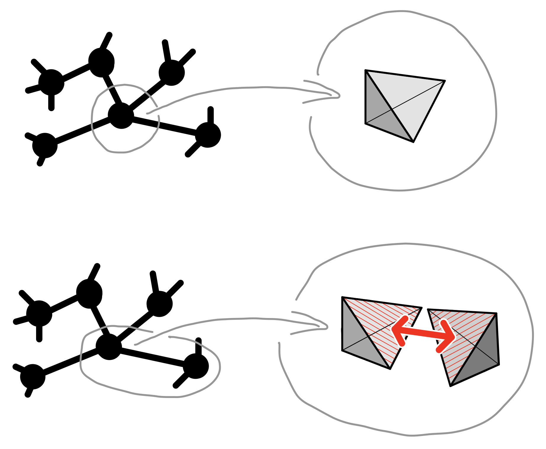
Figure 1: (Top) Each vertex of the logical graph contributes a tetrahedral colex. (Bottom) Each edge contributes a pair of matched facets.

Consider an arbitrary logical graph. The geometry of the resource graph is dictated by a collection of tetrahedral colexes with matched facets, see figure 1:

• There is a tetrahedral colex per vertex of the logical graph.

• If two vertices are linked on the logical graph, the corresponding tetrahedral colexes have a matched facet pair.

The matching establishes a one-to-one relation between the vertices of the two facets that induces a one-to-one relation between edges and faces.

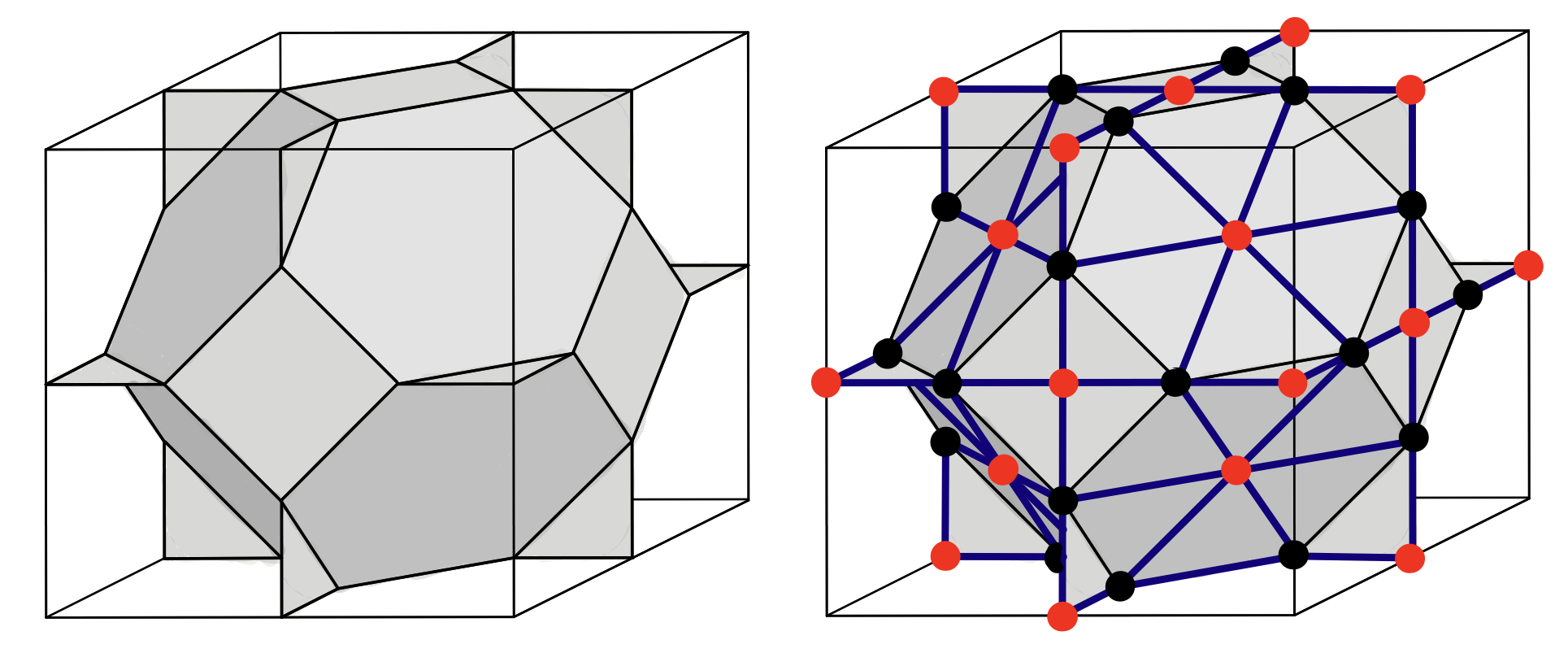
Figure 2: The unit cell for the colex family in Bombin (2015a) (left) and the corresponding resource graph unit cell (right). Code qubits are displayed in black, ancilla qubits in red, and inner edges in purple. Notice that, within the bulk, resource graph vertices are 4- and 6-valent.

The resource state has two kinds of qubits,

• code qubits, one per vertex of the tetrahedral colexes, and

• ancilla qubits, one per face of the tetrahedral colexes,

and two kind of edges in its graph,

• inner edges, connecting each ancilla qubit to each of the code qubits at the ancilla’s face, and

• outer edges, connecting matched code qubits.

Figure 2 illustrates the resource state in the bulk of a colex.

III.2.2 Encoded state

Single-qubit measurements provide the link between the trivial entanglement of the resource state and the global entanglement pattern Chen et al. (2010) that chacterizes the encoded state. Ancilla qubits are always measured in the $X$ basis. The result of measuring the ancillas is the encoded state up to a Pauli frame that depends on the ancilla outcomes and is discussed below. Reorganizing the operations makes this evident:

1. Initialize logical qubits to $|+\rangle$:

   • Initialize code qubits to $|+\rangle$.

   • Measure face operators, i.e.

     • initialize ancilla qubits to $|+\rangle$, and

     • apply a CP gate per inner edge.

2. Apply a logical CP gate per logical edge:

   • Apply a CP gate per outer edge.

III.2.3 Encoded measurements

MBQC on the encoded state proceeds normally. Each logical measurement consists of single-qubit measurements on the code qubits followed by postprocessing:

• If the logical measurement is in a Pauli basis (X, Y or Z), all the code qubits of the tetrahedron are measured in that same basis.

• If the logical measurement is in either of the $X\pm Y$ bases, each code qubit is measured in either of those bases.

Specifically, in the second case the basis choice depends on Bombin (2015a):

• the logical basis: $X+Y$ or $X-Y$,

• the position of the qubit in the tetrahedron, and

• the outcomes of the ancilla qubits of the tetrahedron.

III.3 Pauli frame

The encoded graph state is subject to a Pauli frame that is dictated by the ancilla measurement outcomes. Let these outcomes be represented by the set $\phi$ of ancilla qubits (or equivalently 3-colex faces) with negative outcomes. We regard $\phi$ as a flux configuration, see Bombin . The flux configuration $\phi$ is random, but not completely: in the absence of errors it is an $X$-error syndrome (of the tetrahedral codes).

Upon completion of step 1 of section III.2.2, the result is a collection of encoded $|+\rangle$ states up to a Pauli frame $F_{X}\in P_{X}$ with syndrome $\phi$. Any such Pauli frame can be used, the choice is immaterial. Upon completion of step 2 the Pauli frame has propagated across the CP gates, so that the final Pauli frame is

$$F=F_{X}F_{Z},\qquad F_{Z}\in P_{Z},$$ (2)

where $F_{Z}$ has support on those qubits that are matched to an odd number of qubits where $F_{X}$ has support.

III.3.1 Classical information flow

We denote by

$$f=f_{X}f_{Z},\qquad f_{X}\in P_{X},\,\,f_{Z}\in P_{Z},$$ (3)

the Pauli frame on a given tetrahedron, in contrast with the Pauli frame (2) for the whole system. At each tetrahedron, the flow of classical information in connection with the Pauli frame proceeds as follows:

• The ancilla outcomes are processed to obtain $f_{X}$.

• $f_{Z}$ is obtained from the neighboring tetrahedra.

• If a logical Pauli measurement is performed, the code qubit measurement outcomes are processed together with $f$ to produce a logical outcome ($X$ measurements require $f_{Z}$, $Z$ measurements require $f_{X}$ and $Y$ measurements require both).

• If a logical $X\pm Y$ measurement is performed, $f_{X}$ is used to choose the measurement basis for each code qubit, and the outcomes are processed together with $f_{Z}$ to produce a logical outcome.

The following causal constraints emanate from this information flow:

• Within a tetrahedron measured in the $X\pm Y$ basis, all the ancilla qubits have to be measured before the code qubits are measured.

• The following qubits have to be measured before the logical outcome at a given tetrahedron can be computed:

  • all its code qubits,

  • all its ancilla qubits (except for logical X measurements),

  • all the ancilla qubits of its (matched) neighbors (except for logical $Z$ measurements).

III.4 Fault tolerance

For simplicity, we model noise in the system as follows.

• The (otherwise ideal) resource state is subject to a local distribution of Pauli errors, see (4) below,

• measurements are ideal, but the above errors might depend on the measurement basis, and

• classical computation is flawless.

Such an error model is meaningful only if

• in the logical MBQC scheme, qubits are online for a bounded period of time, and

• the valence of the vertices of the resource graph is bounded.

A distribution of error operators, each with support on a set of qubits $W$, is local with error rate $0\leq p\leq 1$ if for any set of qubits $Q$

$$\text{prob}(Q\subseteq W)\leq p^{|Q|}.$$ (4)

The preparation of the encoded graph state is the crux of the scheme’s fault-tolerance. This is due to its quantum-local nature: it only involves local quantum gates, but the Pauli frame is obtained via global classical computation. There is no reason for the resulting residual noise to follow a local distribution: It is necessary to check that it takes a form that can be handled downstream, when code qubit outcomes are processed.

Stochastic Pauli errors amount to stochastic bit-flip errors on the classical ancilla outcomes. Instead of the correct syndrome $\phi$ the noisy outcome is

$$\tilde{\phi}=\phi+\omega,$$ (5)

where $\omega$ is the set of bit-flip locations, which follow a local distribution. Since $\tilde{\phi}$ is not, in general, a syndrome, it has to be corrected to produce a syndrome $\bar{\phi}$. The syndrome $\bar{\phi}$ determines the Pauli frame $F_{\bar{\phi}}$. The effective error in the Pauli frame is

$$F_{\bar{\omega}}=F_{\phi}F_{\bar{\phi}},\qquad\bar{\omega}:=\phi+\bar{\phi}.$$ (6)

where $F_{\bar{\omega}}$ is any Pauli frame compatible with the syndrome $\bar{\omega}$, and $F_{\phi}$ is the only Pauli frame compatible with the syndrome $\phi$ and the above equation. Recall that a Pauli frame $F$ is defined from its $X$ component $F_{X}$, which is in turn only fixed up to an arbitrary logical operator. This freedom allows adjusting $F_{\phi}$ to the most desirable value of $F_{\bar{\omega}}$.

To recap, $\omega$ follows a local distribution with error rate $p$ and the $X$ component of $F_{\bar{\omega}}$ can be chosen to be correctable, for any given set of correctable errors. Then if the error rate $p$ is below a threshold $p_{0}$, and the corrected syndrome $\bar{\phi}$ is (efficiently) computed as in Bombin (2015b), then the syndrome of $F_{\bar{\omega}}$ is confined, and a fault-tolerant regime exists, see Bombin (2015b, ).

IV Hybrid scheme

The second incarnation of colorful quantum computation is a hybrid scheme: computations are carried out in a two-dimensional setting and quantum information storage requires a third dimension. Optical fiber is particularly well suited to attain this extra dimension. Since stored information is not actively corrected, the fault tolerance of this scheme is not scalable.

A scalable and storage-free two-dimensional approach is discussed in section V. Very loosely speaking, there is a ‘continuum’ of schemes between these two, using increasingly longer storage times.

IV.1 Delayed measurements

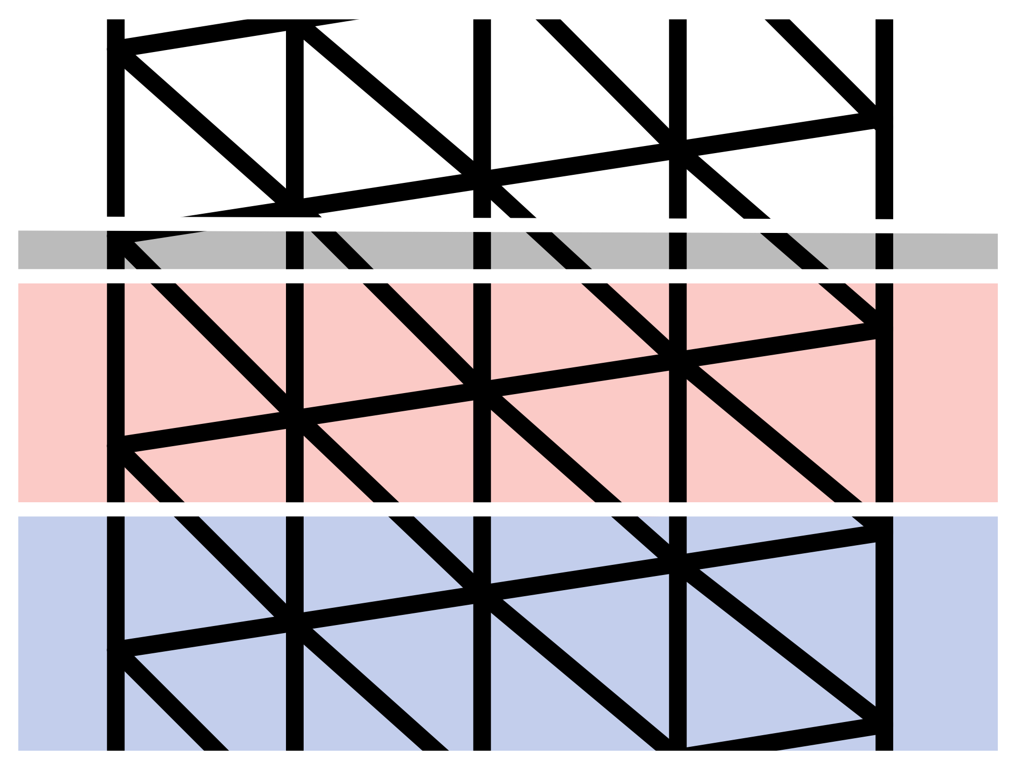
Figure 3: A 2D cut of the 3D MBQC scheme with time as a dimension. Black triangles represent tetrahedra. The colored areas represent regions of the resource state at a point in time. The white one is yet to be created. The grey one is being created. The red one has been created and its ancillas measured. The blue one has been created and all its qubits measured.

As discussed in section II, time cannot be naively exchanged with one of the dimensions of the 3D MBQC scheme of section III. This is due to causal obstructions. The obstacle lies in the flow of classical information, in particular within logical $X\pm Y$ measurements. The Pauli frame $f_{X}$ on the tetrahedron is computed using all the ancilla outcomes, and thus, as noted in section III.3.1, code qubits can be measured only after all the ancilla qubits have been measured.

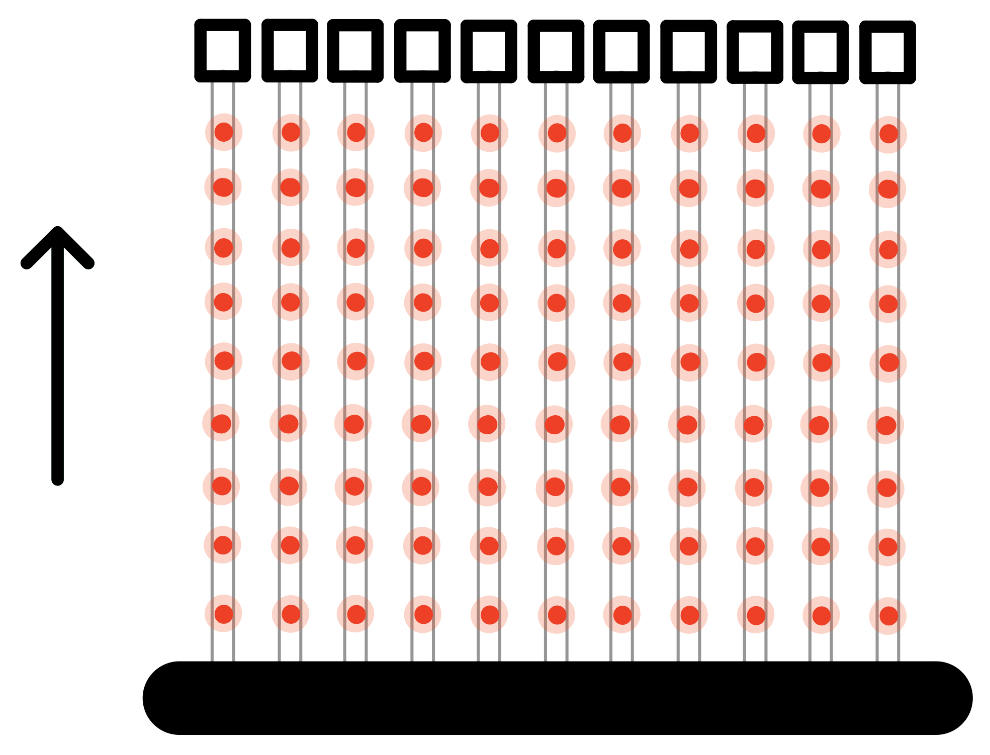
Figure 4: The hybrid scheme requires a 2D computational substrate (lower black region) suplemented with information storage to delay some of the single-qubit measurements (boxes on the top). A natural implementation of the delay/storage is optical fiber (vertical lines). The red dots represent photonic qubits at some instant in time.

The spacetime geometry of this constraint is depicted in figure 4. If the code has distance $L$, the information required to choose the measurement basis for a given code qubit is in general available only after a time proportional to $L$. Code qubits have to ‘sit arround’ for that time before being measured. If the number of qubits required for the 2D computation is $N_{2}$, then the number of online qubits at any given times is

$$N_{3}\propto LN_{2}.$$ (7)

The number of memory qubits required is thus much larger than the number of computational qubits, making the scheme’s appeal strongly implementation dependent. In this regard, an all-important aspect is that the quantum memory used in the scheme is of a rather specific kind.

Qubits are stored for a fixed period of time.

There exists one kind of quantum memory that perfectly matches this scenario: photonic qubits on optical fiber. Figure 4 schematically depicts the resulting architecture. A key feature of optical fiber is that qubits are on the move as they are being stored, which allows to preserve locality in 3D. If the qubits used for storage had a fixed position in time, locality could not be preserved (unless information can be shifted from qubit to qubit locally).

This is not a scalable approach because larger codes requires larger delays. E.g. in the case of optical fiber the maximum storage time is likely dictated by optical loss. Once this maximum is reached, the quality of the delay method has to be improved for larger codes to be useful.

IV.2 Concatenation

In some scenarios the scheme presented here will be concatenated with another scheme capable of e.g. dealing with higher levels of noise. In that case the qubits in storage would likely be encoded. A point to note is that although these qubits are to be measured in either of the $X\pm Y$ bases, any other unitarily equivalent basis pair will do, such as X and Z, which are transversal for any CSS code. E.g. an (encoded) code qubit could first undergo the sequence of gates $P\circ H\circ T$, then enter the delay lines, and finally be measured in either the $X$ or $Z$ basis.

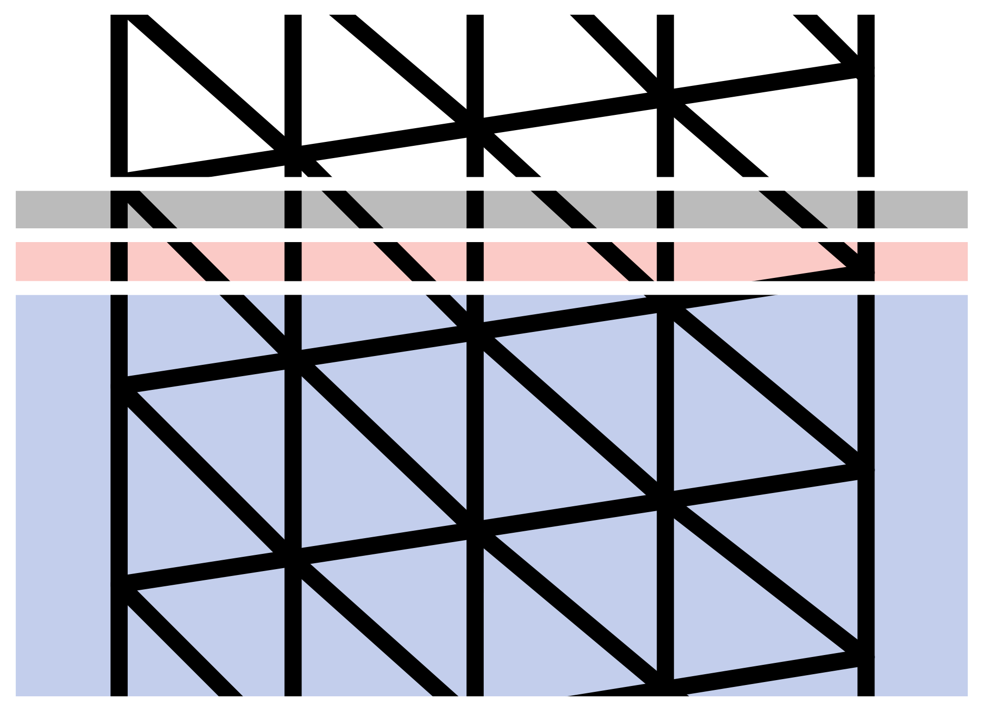
Figure 5: This is a variation of figure 3 in which, at any given time, online qubits are limited to some two-dimensional sublattice of the resource graph.

V 2D scheme

The third and last incarnation of colorful quantum computation is a purely two-dimensional and scalable scheme. We proceed in two steps, first considering the noiseless case and then adding fault tolerance into the mixture, with just-in-time decoding as a key ingredient.

Throughout this section two conditions, involving $X$-error syndromes and time, emerge as necessary for the scheme to function. These conditions are the subject of section VI, which discusses how they constrain the spacetime geometry of tetrahedra. Section VII describes a compatible architecture.

Just-in-time decoders are only formulated here. Section VIII introduces a method to repurpose a conventional decoder for just-in-time decoding.

V.1 Setting

In the 3D MBQC scheme, for each tetrahedral code first all the ancilla measurement outcomes $\phi$ are obtained, and subsequently $f_{X}$, the $X$ component of the Pauli frame, is computed for the whole tetrahedron. We would like to exchange one of the spatial dimensions of the MBQC scheme with time, so that at any given time the qubits that are online form a two-dimensional sublattice, see figure 5. To this end the Pauli frame has to be computed as information becomes available. In particular, the following setting yields a two-dimensional regime.

• Each tetrahedron is divided in layers with bounded width in the time direction. The bound is independent of the size of the computation.

• The Pauli frame $f_{X}$ on the code qubits of a given layer is chosen using the ancilla outcomes of that layer and all the preceding ones.

The following notation is all for a single tetrahedron. On the $i$-th layer,

• $\Lambda_{i}$ is the set of ancillas/faces, and

• $M_{i}$ is the set of code qubits.

Hence at the $i$-th step the accessible ancilla outcomes correspond to the subset of faces

$$\Phi_{i}:=\bigsqcup_{j=1}^{i}\Lambda_{j},$$ (8)

and after the $i$-th step the Pauli frame $f_{X}$ is fixed for the subset of code qubits

$$R_{i}:=\bigsqcup_{j=1}^{i}M_{i}.$$ (9)

The set of all faces is denoted $\Phi$ and the complementary set to $\Phi_{i}$ is

$$\overline{\Phi_{i}}:=\Phi-\Phi_{i}.$$ (10)

V.2 Causality

Even if fault tolerance aspects and the time required for classical computation are ignored, a fundamental issue is whether the outlined scenario is compatible with causal constraints at all. Appendix B provides the following sufficient condition for causality not to be an obstacle. Let $S_{Z}$ denote the subgroup of the tetrahedral code stabilizer generated by face operators. Causality condition. The eigenvalues of $S_{Z}\|_{R_{i}}$ are known at the $i$-th step. As long as the condition holds for every step, it is possible to choose the Pauli frame $f_{X}$ piecewise. The (rather mild) implications of the causality condition for the spacetime geometry are the subject of section VI.2.

V.2.1 Logical causality

Even in the absence of fault tolerance, causality plays a key role in MBQC. In particular, it is not possible to translate directly a given (non-trivial) quantum circuit to a fixed measurement pattern on a graph state. In the original formulation of MBQC it was emphasized that (i) it is possible to fix the measurement basis for all the Pauli measurements, and (ii) on top of those Pauli measurements it is enough to perform $X\pm Y$ measurements. The locations of the $X\pm Y$ measurements is fixed, and only the sign depends on other measurement outcomes, giving rise to causal constraints Raussendorf and Briegel (2001).

The separation between Pauli and non-Pauli measurements is, however, artificial. It is also possible to fix the measurement basis for all non-Pauli measurements and to adjust instead the basis for some Pauli measurements. This can actually be advantageous in fault-tolerant scenarios, because the position of the variable Pauli measurements can be adjusted (delayed) to allow for decoders to process the non-Pauli measurement. This is not possible in the standard formulation of MBQC because the sign of a $X\pm Y$ measurement on a given qubit depends on the outcomes of its neighbors.

Here we adopt the second approach, with fixed non-Pauli measurements, to focus on the problems created by fault-tolerance, rather than logical causality.

V.3 Just-in-time decoding

We are ready to add noise to the picture. In contrast to section III.4, here the corrected syndrome $\hat{\phi}$ has to be generated on the fly, with just a partial knowledge of the noisy ancilla outcomes $\tilde{\phi}$ and with a limited time to perform the computation. This is just-in-time decoding.

V.3.1 The challenge

The goal of JIT decoding is to map, in real time and as information becomes available, the noisy ancilla outcomes $\tilde{\phi}$ to a corrected syndrome $\hat{\phi}$. Each step fixes a partial value for the syndrome $\hat{\phi}$. The input available for this task at the $i$-th step is

$$\tilde{\phi}\cap\Phi_{i}.$$ (11)

For simplicity we assume that this information is used to fix

$$\hat{\phi}\cap\Lambda_{i}.$$ (12)

The partial knowledge of the syndrome $\hat{\phi}$ is then used to choose the Pauli frame $f_{X}$ in the subset of qubits

$$R_{i}-R_{i-1},$$ (13)

following the prescription of appendix B. The consistency of the procedure is guaranteed if the causality condition is satisfied, i.e.

$$S_{Z}\|_{R_{i}}\subseteq S_{\Phi_{i}},$$ (14)

where $S_{\phi_{i}}$ denotes the subgroup of $S_{Z}$ generated by the faces in $\Phi_{i}$.

In the conventional decoding of $\tilde{\phi}$ the relevant classical error correcting code is the set of $X$-error syndromes $\mathcal{C}$. By contrast, when the known ancilla outcomes are those in the subset $\Phi_{i}$ the natural code to consider is

$$\mathcal{C}_{i}:=\{\phi\subseteq\Phi_{i}\,|\,\exists\phi^{\prime}\subseteq\overline{\Phi_{i}}\,:\,\phi+\phi^{\prime}\in\mathcal{C}\}.$$ (15)

The $i$-th step of JIT decoding is not only limited by the lack of knowledge of the future ancilla outcomes, but also by the previous commitment to a final value of $\hat{\phi}$ in the subset $\Phi_{i-1}$. A straightforward method to overcome this difficulty is the subject of section VIII, but it is likely that better ones exist.

V.3.2 The penalty

Dealing with the noisy flux configuration $\tilde{\phi}$ on a layer by layer basis makes correcting errors harder. With full access to $\tilde{\phi}$ a conventional decoder produces a better estimate $\bar{\phi}$. Fortunately it is possible to attenuate the damaged caused by using $\hat{\phi}$, rather than $\bar{\phi}$, to choose the Pauli frame $f_{X}$.

Conventional decoding enhances the logical outcome processing.

In particular, since $\bar{\phi}$ is the best estimate for the syndrome, it is natural to consider the differential syndrome

$$\delta:=\hat{\phi}+\bar{\phi}.$$ (16)

Were $\bar{\phi}$ correct, using the wrong syndrome $\hat{\phi}$ would introduce some effective noise. The code qubit measurements can be regarded as a transversal unitary followed by single qubit $X$ mesurements. In this picture, the effective noise amounts to the following errors right before the $X$ measurements:

• a known $Z$ Pauli error that can trivially be compensated for, and

• a random element of a certain group $H(\delta)\subseteq P_{Z}$ with generators localized in the vicinity of the faces in $\delta$. Such random noise is very similar to qubit erasure, and can be handled analogously.

Notice that in the adjacent tetrahedra the Pauli frame should be dictated by $\bar{\phi}$, rather than $\hat{\phi}$,to avoid propagating JIT decoding errors between tetrahedra.

V.4 Closure

This section discusses a geometrical counterpart to the causality condition, which is of a topological nature. The new condition emerges naturally upon examination of the JIT decoder presented in section VIII, where it is required to achieve fault tolerance. However, it is presented here since, unless it is satisfied, it seems unlikely that a JIT decoder can be successful.

Given a familty of encodings for the fault-tolerant scheme under discussion, the following condition needs to be satisfied for some $k_{\text{close}}$, every tetrahedral colex in the family, and each layer $i$. Closure condition. For every $\phi\in\mathcal{C}_{i}$ there exists $\phi^{\prime}\subseteq\overline{\Phi_{i}}$ such that

$$|\phi^{\prime}|\leq k_{close}|\phi|,\qquad\phi+\phi^{\prime}\in\mathcal{C}.$$ (17)

Intuitively, the closure condition states that committing to some value of $\hat{\phi}\cap\phi_{i}$ should not have disproportionate side effects. If not satisfied, small errors in early stages could get amplified and spoil fault-tolerance. Section VI.3 explores the implications of the closure condition for the spacetime geometry.

VI Spacetime geometry

This section discusses how to ensure that the causality and closure conditions encountered in section V are satisfied. The closure condition imposes significant restrictions to the spacetime geometry of tetrahedral colexes. Section VII introduces a symmetrical architecture in which all tetrahedra satisfy them.

VI.1 Setting

There are many ways in which the layers of section V.1 could be defined. For simplicity, we define layers in terms of sets of (3-)cells. Namely, for each $i=1,\dots,n$ there is a set of cells $C_{i}$ with

$$C_{1}\subset C_{2}\subset\dots\subset C_{n},$$ (18)

where $C_{n}$ is the set of all cells. The choice of $C_{i}$ dictates the content of each layer, and thus the causal structure. In the notation of section V.1:

• The code qubits in $R_{i}$ are those at a vertex of any cell in $C_{i}$.

• The ancilla qubits in $\Phi_{i}$ are those at a face of any cell in $C_{i}$.

VI.2 Causality condition

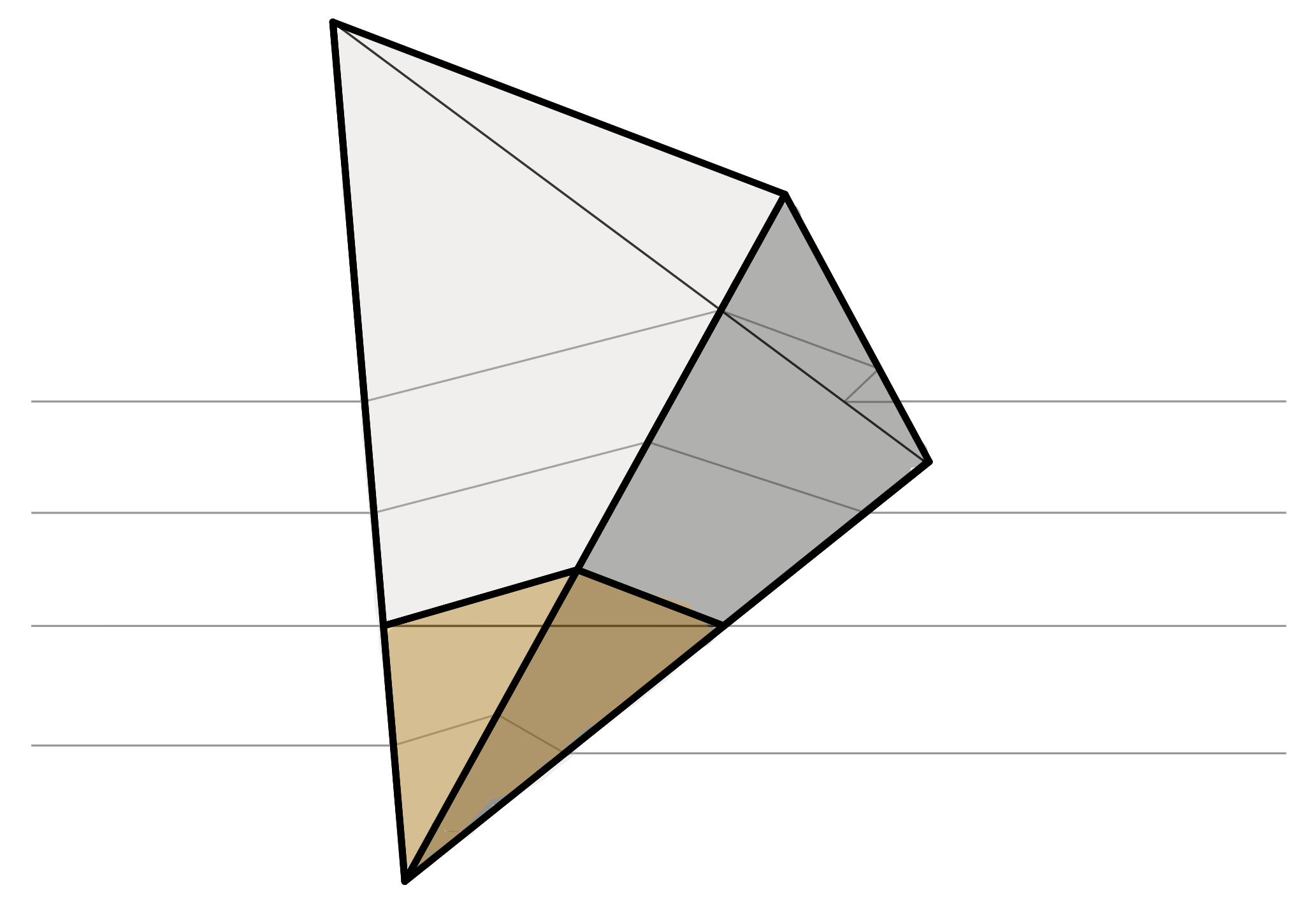
Figure 6: Time runs upwards. Horizontal lines are a guide to the eye. The highlighted region of the tetrahedron corresponds to the set of cells $C_{i}$. The topological constraints imposed by the causality condition are easily satisfied irrespective of the orientation of the tetrahedron.

The proof of the following result is in appendix C.

Lemma 1.

The causality condition is satisfied if

• the submanifold formed by the cells in $C_{i}$ is a topological ball, and

• its intersection with each cell outside $C_{i}$, and with each facet of the tetrahedral colex, is empty or a topological disc.

The causality condition holds for reasonable geometries. E.g. if the facets of the tetrahedra are aproximately flat, see figure 6.

VI.3 Closure condition

This condition poses more of a challenge: some care is needed in choosing the spacetime geometry of each tetrahedron.

VI.3.1 Dual graph distances

Figure 7: A 2D analogue of the dual graph $\Gamma$. The orange faces of the 2-colex play the role of the set of cells $C_{i}$ in the 3-colex, and the triangle edges the role of tetrahedron facets. The dual graph $\Gamma_{i}$ appears in orange, and $\overline{\Gamma_{i}}$ in grey. The highlighted vertex $v$ has $d_{\text{blue}}(v)=3$, $\overline{d_{\text{blue}}}(v)=\infty$ and $\overline{d}(v)=5$.

The dual graph $\Gamma$ describes error syndromes in tetrahedral codes Bombin : its vertices are dual to the cells of the 3-colex, and its edges are dual to the faces of the 3-colex and represent flux elements. Edges that are dual to a face belonging to a facet of the colex have a missing vertex, and we consider them to be connected to the facet.

Let $\Gamma_{i}$ (respectively $\overline{\Gamma_{i}}$) denote the subraph of $\Gamma$ with edges dual to the faces in $\Phi_{i}$ (respectively $\overline{\Phi_{i}}$). For each $i$, we introduce the following distance functions for vertices in $\Gamma_{i}$, see figure 7. Given any vertices $v,v^{\prime}$ of $\Gamma_{i}$ and a color $\kappa$,

• $d(v,v^{\prime})$ is the distance between $v$ and $v^{\prime}$,

• $d_{\kappa}(v)$ is the shortest distance from $v$ to any $\kappa$-colored facet, and

• $d(v)$ is the sum of the two smallest values of $d_{\kappa}(v)$ among the 4 values for varying color $\kappa$.

Barred versions $\overline{d}(v,v^{\prime})$, $\overline{d}_{\kappa}(v)$ and $\overline{d}(v)$ are defined analogously for $\overline{\Gamma_{i}}$.

VI.3.2 Forbidden geometries

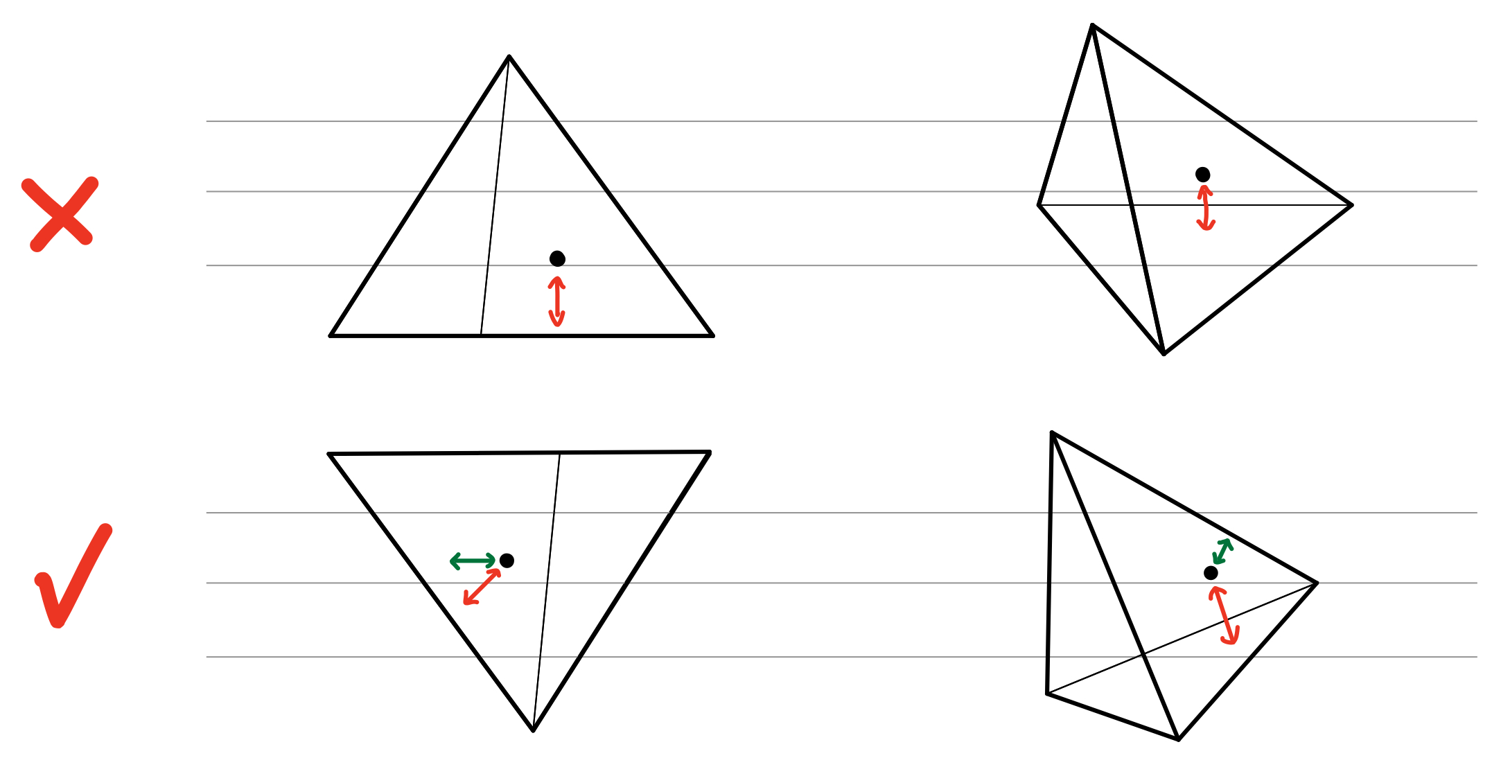
Figure 8: Examples of spacetime geometries and the obstructions created by the closure condition. Time runs upwards. Horizontal lines are a reminder of the layered structure. (Top) In both examples there are vertices $v$ such that for some $\kappa$ the distance $d_{\kappa}(v)$ (the red arrow) is very small while $\overline{d_{\kappa}}(v)$ and $\overline{d}(v)$ are proportional to the size of the tetrahedron. The existence of such vertices is due to the fact that at some point in time a whole facet, or a last remaining edge of it, disappears suddenly. (Bottom) These geometries are compatible with the closure condition (assuming that the facet gradients are bounded from below across the family of colexes of interest). In the first example a small value of $\overline{d_{\kappa}}(v)$ saves the day, whereas in the second case $\overline{d}(v)$ makes the difference for some vertices, as the one depicted.

Lemma 2.

If the cells of the tetrahedral colex have at most $k_{\text{face}}$ faces and

• for every cell $c\not\in C_{i}$ the set of points of $c$ that also belong to some element of $C_{i}$ is simply connected, and

• for any color $\kappa$ and any vertices $v,v^{\prime}$ of $\Gamma_{i}$

  $$\overline{d}(v,v^{\prime})\leq k\,d(v,v^{\prime}),$$ (19)

  $$\min\left(\overline{d_{\kappa}}(v),\overline{d}(v)\right)\leq k\,d_{\kappa}(v),$$ (20)

then the closure condition is satisfied for

$$k_{\text{close}}=4k(k_{\text{face}}-1).$$ (21)

The proof is in appendix D. Neither the first condition nor the first inequality are a big source of difficulties. Assuming that the lattice is regular enough, the first inequality holds for some $k$ (independent of the code size) as long as the $\Phi_{i}$-to-$\overline{\Phi_{i}}$ interfaces are simply connected and approximately flat and convex. The second inequality, however, forbids certain overall geometries. This is illustrated in figure 8.

VII Twister architecture

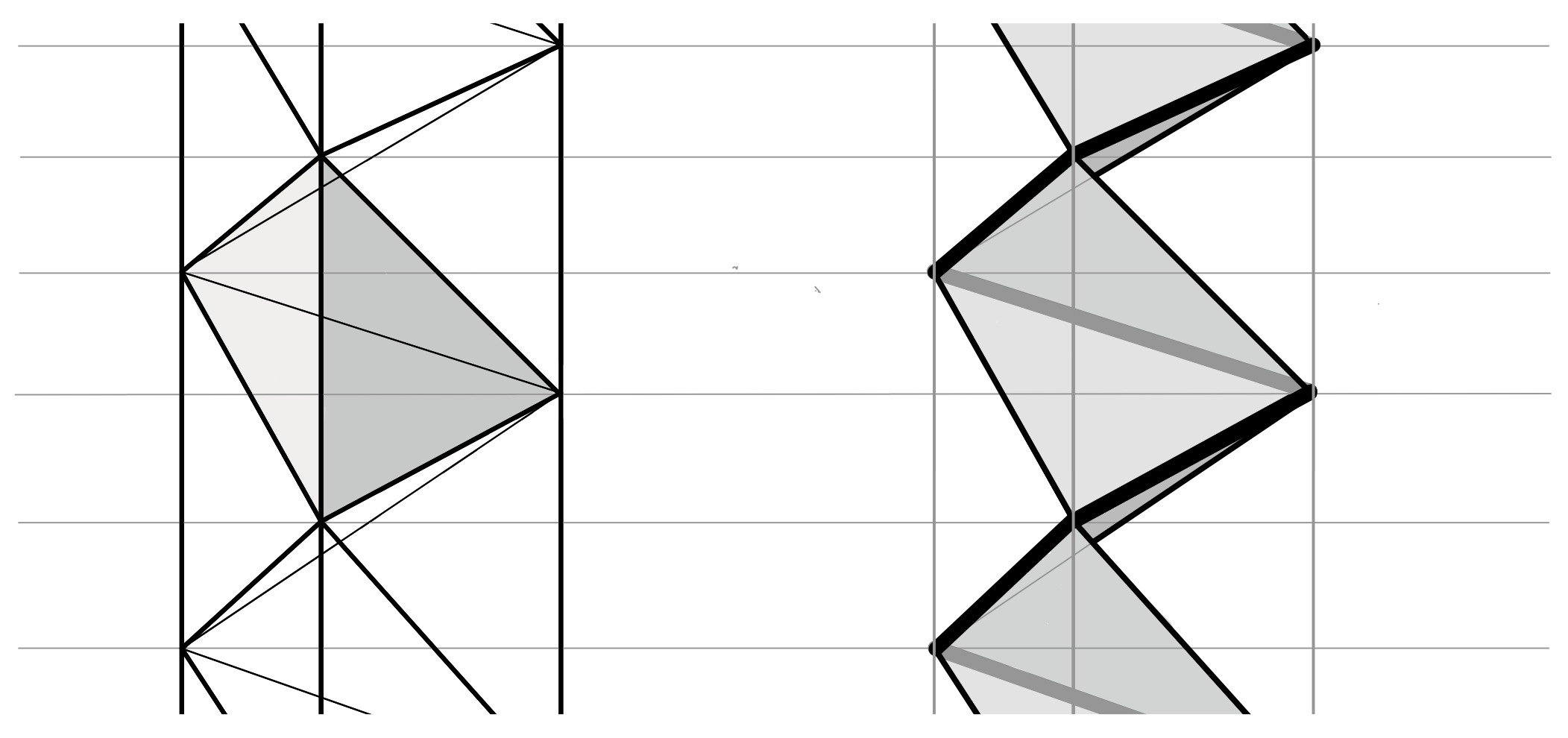
Figure 9: Lateral projection of the ‘twister’ arrangement of tetrahedra on a prism. The tetrahedra are related by a discrete helicoidal symmetry. The horizontal lines are a guide to the eye. (Left) A single tetrahedron is highlighted. (Right) The inner facets, those separating the tetrahedra, are shaded, and the edges along which these facets meet are highlighted.

This section introduces a symmetrically arrangement of tetrahedra compatible with the geometrical conditions of section VI.

VII.1 Linear logical graph

Linear graph states enable MBQC for a single computational logical qubit. As shown in figure 9, the corresponding tetrahedra can be arranged on a ‘twister’ geometry: filling up a prism according to a discrete helicoidal symmetry. For the hybrid and two-dimensional schemes the time direction is the prism’s axis, i.e. the direction along which the logical computation proceeds. Notice that the spacetime geometry of each tetrahedron corresponds to one of the cases in figure 8.

VII.2 Multi-qubit computation

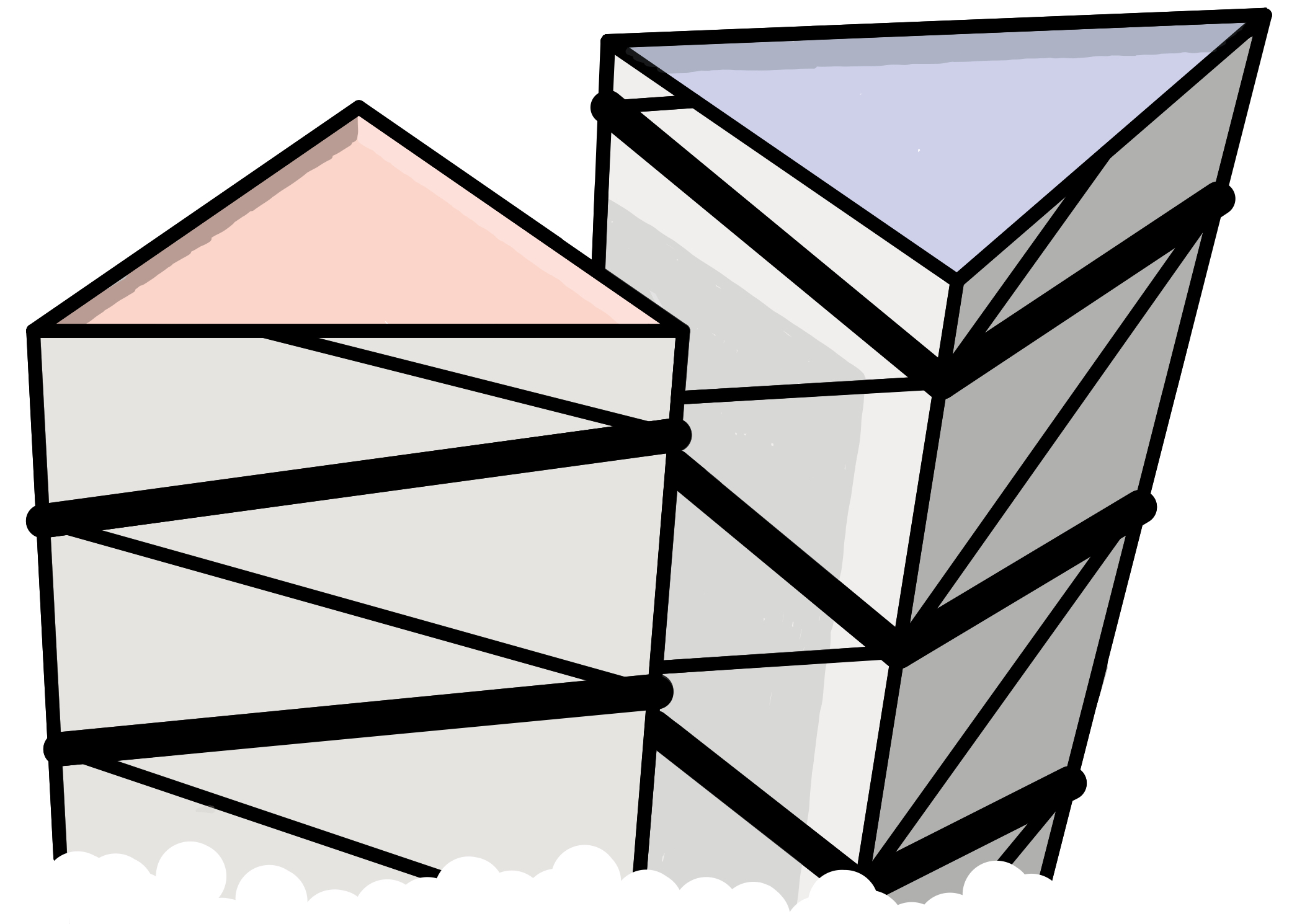
Figure 10: Two ‘twister’ configurations of tetrahedra with opposite chirality. Each contributes a logical computational qubit. When placed side by side the facets can be matched, enabling 2-qubit logical gates. Some edges are highlighted to make the symmetry more apparent.

As suggested in figure 10, two ‘twister’ arrangements of tetrahedra can be placed side by side as long as they have opposite chirality. They can be arranged in a row or fill the whole space, see figure 11. In the former case the resulting logical graph state is planar, see figure 12. From the circuit model perspective this enables computation on a logical one-dimensional array. In the latter case the resulting graph is three-dimensional, which corresponds to computation on a two-dimensional array of logical qubits. In both cases the topology of the logical graph can be modified by removing some edges, i.e. by not matching the corresponding facets in the construction of the resource state.

Figure 11: Possible arrangements of ‘twisters’. Each twister contributes a logical computational qubit, and thus the pattern also reflects the topology of the logical circuit. (Left) A single row. (Right) A space-filling pattern.

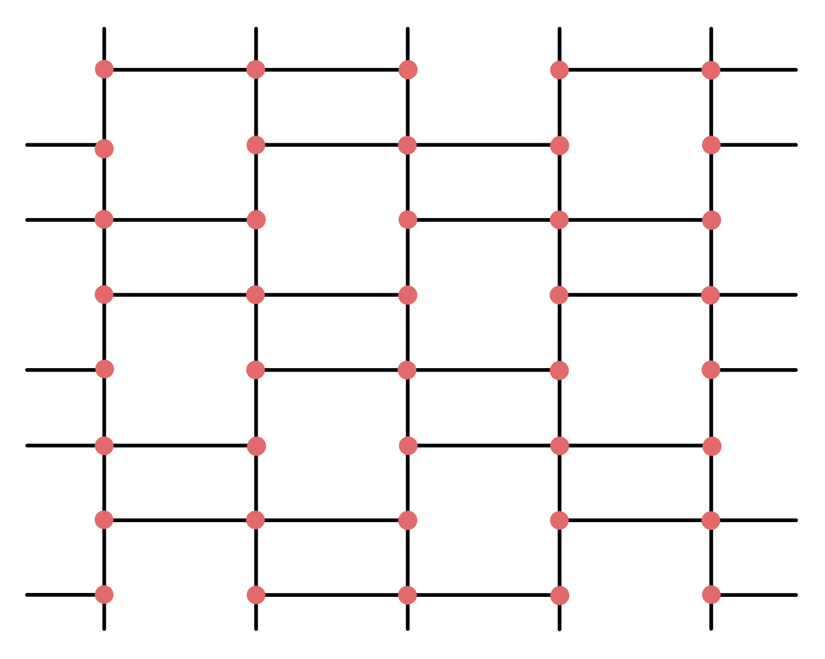
Figure 12: The logical graph resulting of the arrangement of figure 11 (left).

The three dimensional logical graph resulting from the space-filling pattern of figure 11 (right) is dual to a 3-colex. Thus, the twister architecture enables to have a single symmetry govern both the overall geometry of the tetrahedral colexes and the geometry of the underlying 3-colex lattice.

VIII Naive JIT decoder

This section introduces a JIT decoder that, at each step and using conventional decoders,

• estimates a portion of the $X$-error syndrome with the available information, and

• compensates for the difference between the current estimate and the one made in the previous step.

This ‘naive’ approach is fault tolerant.

VIII.1 Simplification

We adopt the following simplifying assumption for decoding processes.

Classical computation and communication are instantaneous.

In the limit of large systems, this is unphysical. The time required for decoding grows with the code size, whereas the available time is by assumption independent of the code size. Similarly, as the code size grows information becomes farther spread in space, but information can only travel at a finite speed.

We only consider decoding tasks for which there exist efficient algorithms. Moreover, it is likely that these tasks can also be successfully accomplished under tight physical assumptions. Indeed, both renormalization group Duclos-Cianci and Poulin (2010); Sarvepalli and Raussendorf (2012); Duclos-Cianci and Poulin (2013) and cellular automaton Herold et al. (2015, 2017); Dauphinais and Poulin (2017); Kubica and Preskill (2010) ideas have already been applied in very similar scenarios.

VIII.2 Decoding problem

Consider the decoding problem posed by the linear code $\mathcal{C}$ formed by $X$-error syndromes. A decoder $D$ for this code is a map

$$D:\mathcal{P}(\Phi)\longrightarrow\mathcal{C}.$$ (22)

where $\Phi$ is as in section V.1. It satisfies for any $\phi\in\mathcal{C}$ and any $\omega\subseteq\Phi$,

$$D(\omega+\phi)=D(\omega)+\phi.$$ (23)

I.e. the decoder estimates an error based solely on the sydrome of its input. The decoders considered below are assumed to satisfy analogous conditions.

VIII.2.1 $\mathbf{Z}_{2}$ charge decoding.

The decoding problem above is a $\bf Z_{2}^{3}$ analogue of the $\bf Z_{2}$ problem faced in the fault-tolerant correction of $X$ (or $Z$) errors in the 2D toric code (with an important difference to be noted below). In particular, it is possible to map the former problem to the later at the cost of a constant factor in the weight of the decoded errors Bombin (2015b). Since the $\mathbf{Z}_{2}$ case is simpler and well known, we use it to illustrate the naive JIT decoder.

The $\mathbf{Z}_{2}$ decoding problem is as follows Dennis et al. (2002), see also appendix E.4.1. There is a 3D lattice with set of edges $E$. The code is formed by closed sets ($\mathbf{Z}_{2}$ chains) of edges, and the inputs for decoding are arbitrary sets of edges $E$. In the case of fault-tolerant error correction in the toric code, only the homology class of the decoded set of edges is relevant, whereas for the JIT decoder it is the actual codeword that matters. The difference is, however, immaterial if the decoder approximates the most likely error (as in minimum weight matching Dennis et al. (2002)), rather than the most likely equivalence class.

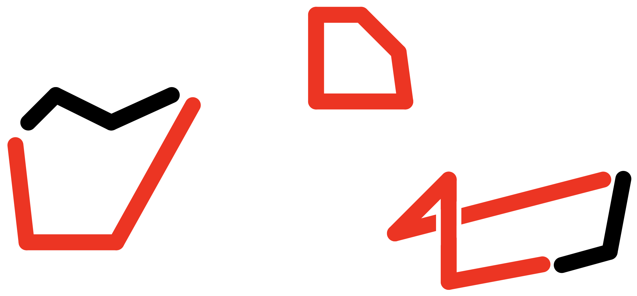
Figure 13: The goal of the $\mathbf{Z}_{2}$ charge decoding problem is to find a likely error (black set of edges) with the same endpoints as the actual error (red).

The errors involved in the process are as follows. The input is some subset of edges $\tilde{e}\subseteq E$. Suppose that it takes the form $e+\omega$, where $e$ is a codeword and $\omega$ the error. The error syndrome is extracted from $\tilde{e}$: it is the set of endpoints of $\tilde{e}$, which coincide with the endpoints of $\omega$. Decoding amounts to choose some $\omega^{\prime}$ with the same endpoints as $\omega$, see figure 13:

$$e+\omega\quad\overset{D}{\longmapsto}\quad e+(\omega+\omega^{\prime}).$$ (24)

The residual error is $\omega+\omega^{\prime}$.

VIII.3 Adapted decoders

The naive JIT decoder requires two modified versions of the decoder $D$. Recall the layer structure introduced in section V.1. For each layer $i$ we consider

• a decoder $D_{i}$ for errors in $\Phi_{i}$ with open boundary conditions, used for the $i$-th estimating step, and

• a decoder $\overline{D_{i}}$, based on a decoder for errors in $\overline{\Phi_{i}}$ with closed boundary conditions, and used for the $(i+1)$-th compensating step.

‘Boundary’ here refers to the interface between $\Phi_{i}$ and $\overline{\Phi_{i}}$, which in practice takes the form of a 2D sheet separating the first $i$ layers from the rest.

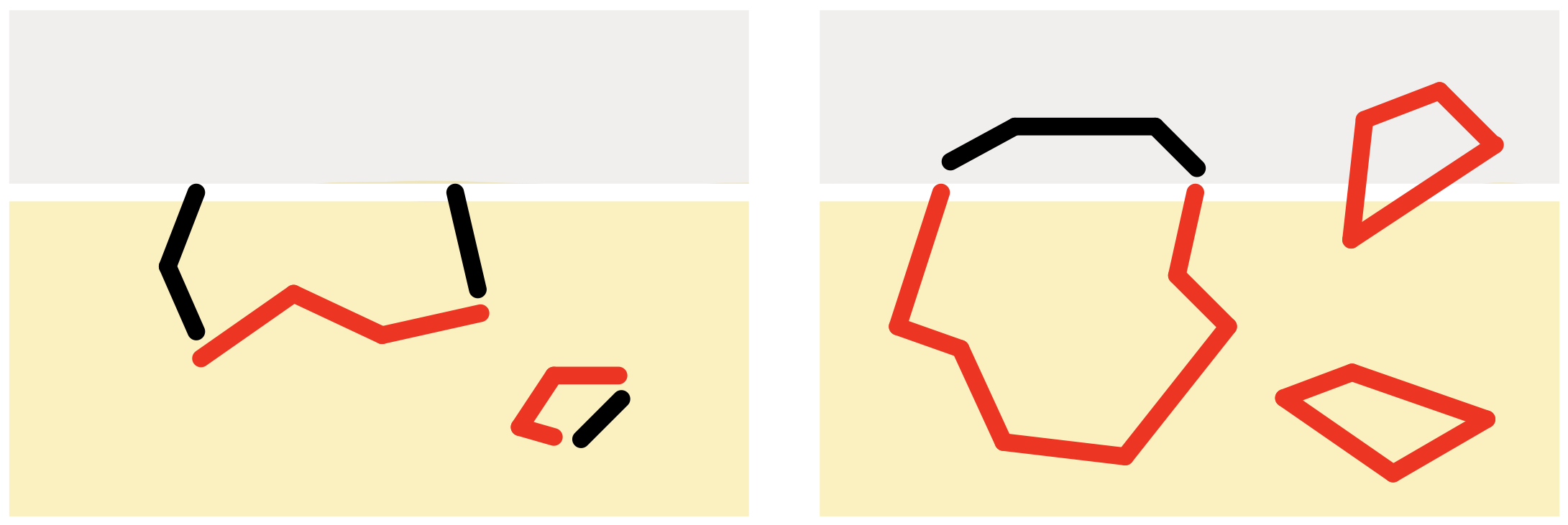
Figure 14: The workings of the decoders $D_{i}$ (left) and $\bar{D}_{i}$ (right). The orange and grey regions represent $\Phi_{i}$ and $\overline{\Phi_{i}}$ respectively. The sets of edges $\omega$ and $\omega^{\prime}$ are represented in red and black, respectively, see equations (26) and (33).

The open boundary conditions decoder is a function

$$D_{i}:\mathcal{P}(\Phi_{i})\longrightarrow\mathcal{C}_{i}.$$ (25)

For this decoder the original decoding problem is modified by imposing that for any $\omega\subseteq\Phi_{i}$ and $\gamma\subseteq\overline{\Phi_{i}}$, the error $\omega+\gamma$ is as likely as the error $\omega$. Thus it is meaningful to have subsets of $\Phi_{i}$ as both input and output: the $\overline{\Phi_{i}}$ component is completely random and irrelevant. It is in this sense that the boundary conditions are open, see appendix D.5. Decoding takes the form

$$\phi\cap\Phi_{i}+\omega\quad\overset{D_{i}}{\longmapsto}\quad\phi\cap\Phi_{i}+\omega+\omega^{\prime},$$ (26)

where the input is composed by some $\phi\in\mathcal{C}$ and an error $\omega\in\Phi_{i}$. In the $\mathbf{Z}_{2}$ picture, illustrated in figure 14 (left), $\omega$ and $\omega^{\prime}$ share endpoints except possibly at the interface of $\Phi_{i}$ and $\overline{\Phi_{i}}$. .

The closed boundary conditions decoder is a function

$$D_{i}^{\prime}:\mathcal{P}\left(\overline{\Phi_{i}}\right)\longrightarrow\mathcal{C}\cap\mathcal{P}\left(\overline{\Phi_{i}}\right).$$ (27)

For this decoder the original decoding problem is constrained to the subset of edges $\overline{\Phi_{i}}$: these are the only noisy ones. Rather than using this decoder directly, it will be used in the ‘compensating’ step, as indicated above. To this end, let us recast it as

$$D_{i}^{\prime}(\phi)=:\phi+E_{i}(\phi),$$ (28)

where $E_{i}$ is a function that only depends on the syndrome of its argument and yields a Pauli operator with that syndrome, i.e. $E_{i}(\phi)$ is the estimated error for $\phi$.

The closure decoder is the function

$$\overline{D_{i}}:\mathcal{C}_{i}^{\prime} \longrightarrow\mathcal{C},$$ (29)

$$\phi \longmapsto\phi+E_{i}(\phi),$$ (30)

with domain

$$\mathcal{C}_{i}^{\prime}:=\{\phi+\omega\,|\,\phi\in\mathcal{C},\,\,\omega\in\mathcal{C}_{i}\}.$$ (31)

Notice that only the $\overline{\Phi_{i}}$ component of $\phi$ is modified, i.e. for every $\phi\in\mathcal{C}_{i}^{\prime}$

$$\phi+\overline{D_{i}}(\phi)\,\in\overline{\Phi_{i}}.$$ (32)

The $\Phi_{i}$ component of the input sets the boundary conditions to be satisfied by the $\overline{\Phi_{i}}$ component of the output, which ‘closes the open ends’. Decoding takes the form

$$\phi+\omega\quad\overset{\overline{D_{i}}}{\longmapsto}\quad\phi+(\omega+\omega^{\prime}),$$ (33)

where $\phi\in\mathcal{C}$, $\omega\in\mathcal{C}_{i}$ and $\omega^{\prime}\in\overline{\Phi_{i}}$. In the $\mathbf{Z}_{2}$ picture, illustrated in figure 14 (right), $\omega$ and $\omega^{\prime}$ share endpoints.

Appendix D.5 provides a simple criteria guaranteeing that ‘open’ boundary conditions are truly so. For reasonable partitions of the lattice into layers it should in general be straightforward to adapt any decoding algorithms $D$ in order to obtain algorithms $D_{i}$ and $\overline{D_{i}}$. Indeed, the situation is not conceptually different from the well known ‘smooth’ and ‘rough’ boundaries in toric codes.

VIII.4 Computation

At the $i$-th layer the naive JIT decoder produces a syndrome $\hat{\phi}$ of the form

$$\hat{\phi}\cap\Lambda_{i}:=\gamma_{i}\cap\Lambda_{i},$$ (34)

where $\gamma_{i}$ is computed, as stated above, in two steps, estimation

$$\gamma_{i}^{\prime}:=D_{i}(\tilde{\phi}\cap\Phi_{i})$$ (35)

and compensation

$$\gamma_{i}:=\gamma_{i}^{\prime}+\overline{D_{i-1}}(\gamma_{i-1}+\gamma_{i}^{\prime}\cap\Phi_{i-1}).$$ (36)

with $\gamma_{0}:=\emptyset$. The above is well defined because $\gamma_{i}\in\mathcal{C}_{i}^{\prime}$. It is not difficult to check that

$$\hat{\phi}\cap\Phi_{i}=\gamma_{i}\cap\Phi_{i}.$$ (38)

It is worth pointing out that the same decoders can be used when information from farther layers is available, by settling on the values of $\hat{\phi}$ for a single layer but computing with all the available layers.

VIII.5 Errors

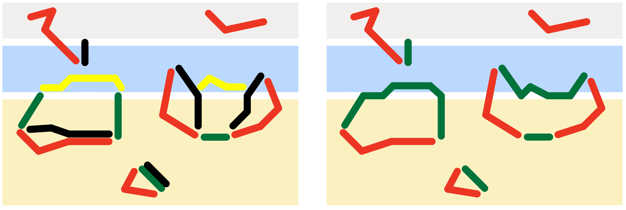
Figure 15: The workings of the naive JIT decoder. The orange, blue and grey region represent $\Phi_{i-1}$, $\Lambda_{i}$ and $\overline{\Phi_{i}}$, respectively. The sets of edges $\omega$ is represented in red, $\omega_{i}^{\prime}$ in black, $\epsilon_{i}$ in yellow, $\omega_{i-1}$ in green (left only) and $\omega_{i}$ in green (right only). See equations (39-43).

Let us rephrase the computation in terms of several different kinds of ‘errors’.

Let $\phi\in\mathcal{C}$ be the noiseless flux configuration (a syndrome) and $\tilde{\phi}\subseteq\Phi$ the noisy one. We define

• the error $\omega$ in the measurements

  $$\omega:=\phi+\tilde{\phi},$$ (39)

• the residual error $\hat{\omega}$ of JIT decoding

  $$\hat{\omega}:=\phi+\hat{\phi},$$ (40)

• the estimated error $\omega_{i}^{\prime}$ at the $i$-th step

  $$\omega_{i}^{\prime}:=\gamma^{\prime}_{i}+\tilde{\phi}\cap\Phi_{i},$$ (41)

• the effective estimated error $\omega_{i}$ at the $i$-th step

  $$\omega_{i}:=\gamma_{i}+\tilde{\phi}\cap\Phi_{i},$$ (42)

• the compensating flux configuration $\epsilon_{i}$ at the $i$-th step

  $$\epsilon_{i}:=E_{i}\left(\gamma_{i-1}+\gamma_{i}^{\prime}\cap\Phi_{i-1}\right).$$ (43)

A crucial property is that, since $\gamma_{i}$ and $\gamma_{i}^{\prime}$ have the same syndrome, $\epsilon_{i}$ only depends on the estimated errors of two consecutive guessing steps:

$$\epsilon_{i}=E_{i}\left(\omega_{i-1}^{\prime}+\omega_{i}^{\prime}\cap\Phi_{i-1}\right).$$ (44)

The corresponding $\mathbf{Z}_{2}$ picture is illustrated in figure 15: $\omega_{i}^{\prime}$ (and thus $\omega_{i}$) has the same endpoints as $\omega\cap\Phi_{i}$, except at the interface separating $\Phi_{i}$ and $\overline{\Phi_{i}}$. The expressions 35 and 36 can be restated in terms of these various errors,

$$\omega_{i}^{\prime} =\omega\cap\Phi_{i}+D_{i}(\omega\cap\Phi_{i}),$$ (45)

$$\omega_{i} =\omega_{i-1}+\omega_{i}^{\prime}\cap\Lambda_{i}+\epsilon_{i},$$ (46)

and the residual error of JIT decoding is

$$\hat{\omega}=\omega_{n}=\sum_{i}\left(\omega_{i}^{\prime}\cap\Lambda_{i}+\epsilon_{i}\right).$$ (47)

VIII.6 Fault tolerance

Under the same assumptions as in section III.4, the naive JIT decoder makes the 2D scheme fault tolerant. As discussed next, this is true in particular

• for decoders with an efficient implementation, and

• in an unfavorable scenario that omits the strategy of section V.3.2.

Just as in the three-dimensional scenario, the preparation of the encoded graph state is the crux of the scheme’s fault-tolerance. In this case there is an additional complication: the residual error of JIT decoding (47) does not seem amenable to the ‘confined syndromes’ approach of Bombin (2015b, ).

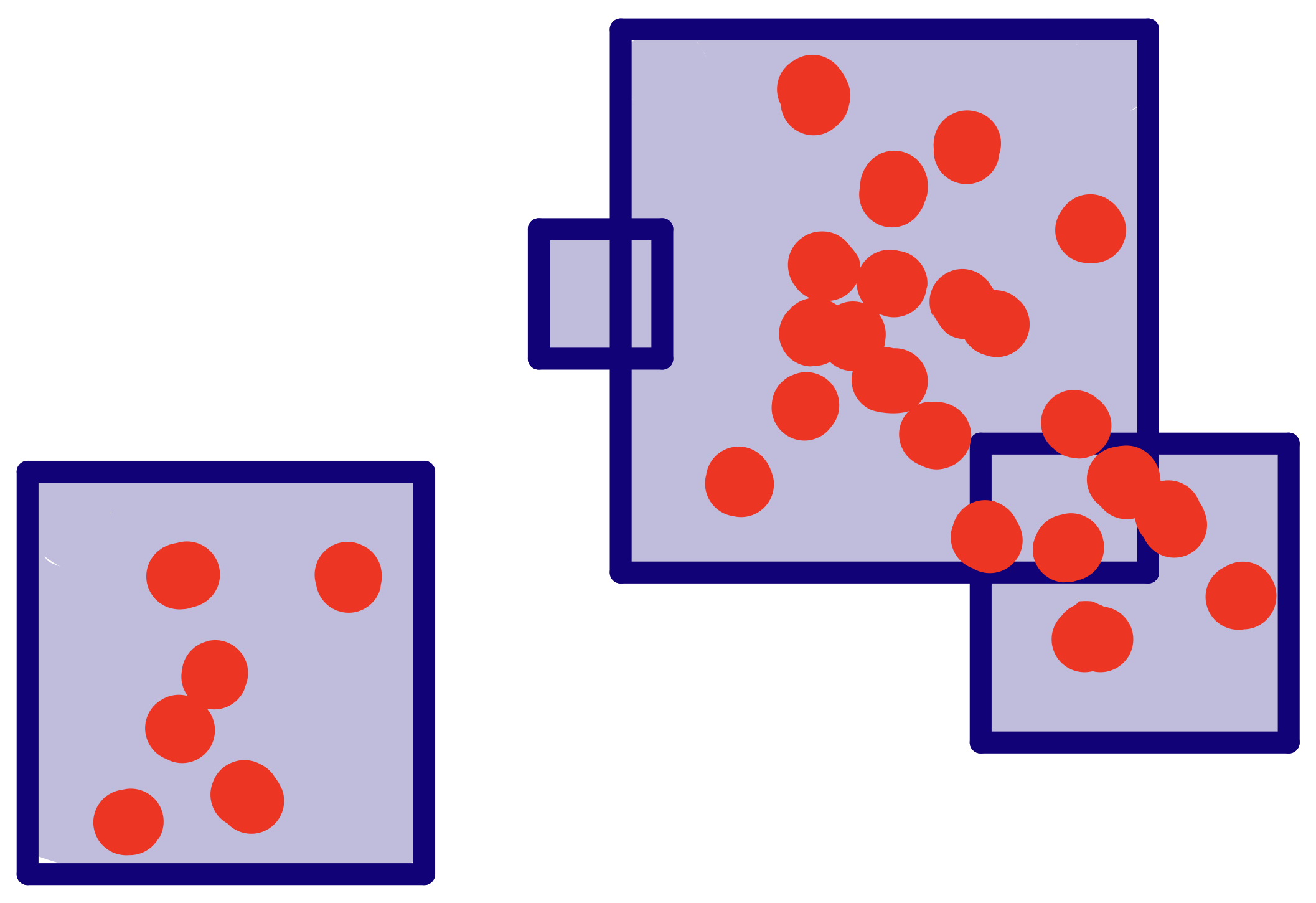
Figure 16: Errors (red dots) confined to the interior of a collection of balls.

The workaround is to consider an alternative to local noise that is well-suited to topological codes. The key element are geometrical balls, defined by some metric that reflects the structure of errors and syndromes. It is assumed that that each error $e$ is mapped to a ball set $W$ such that the support of $e$ is contained within the balls in $W$, see figure 16. Ball-local noise is defined in terms of the distribution of balls $W$.

A distribution of error operators, each with support constrained to the interior of some set of balls $W$, is ball-local with rate $0\leq p\leq 1$ if for any set of balls $B$

$$\text{prob}(B\subseteq W)\leq p^{r(B)},$$ (48)

where $r(B)$ is the sum of the radii of the balls in $B$.

Notice that $\hat{\omega}$ is the JIT counterpart to the error $\bar{\omega}$ of section III.4. By the same argument used for $\bar{\omega}$, the $X$ component of the effective Pauli frame error $F_{\hat{\omega}}$ is only fixed up to a logical error. The following result, technically stated in theorem 15, assumes that (see appendix VIII for details)

• the closure condition holds,

• the family of tetrahedral colexes has a uniform local structure (such as the one described in Bombin (2015a)), and

• the decoders $D_{i}$ and $D_{i}^{\prime}$ satisfy certain technical conditions (satisfied for the decoder $D$ described in Bombin (2015b)).

If the error rate for ancillas outcomes is below a threshold $p_{0}$, the $X$ component of $F_{\hat{\omega}}$ follows a ball-local distribution with rate

$$\left(\frac{p}{p_{0}}\right)^{k},$$ (49)

where both $p_{0}$ and $k$ depend on the local structure of the colexes and on the decoders $D_{i}$, $D_{i}^{\prime}$.

When the $X$ component of $F_{\hat{\omega}}$ follows a ball-local distribution, so does $F_{\hat{\omega}}$ too, because it is obtained from its $X$ component via (local) logical CP gates. Observe that the code qubits measurements affected by $F_{\hat{\omega}}$ do not belong to logical qubits measured in the $Z$ basis. Therefore, the logical outcome processing affected by $F_{\hat{\omega}}$ always involves a $\mathbf{Z}_{2}^{3}$ charge decoder. This decoding problem can be mapped to three connected copies of the $\mathbf{Z}_{2}$ charge problem Bombin (2015b); Kubica et al. (2015). This mapping preserves the ball-local character of the error distribution. Appendix E.4 shows that, for the $\mathbf{Z}_{2}$ charge problem, there exist efficient decoders with an error correction threshold for ball-local noise. Thus, fault-tolerance is indeed feasible.

IX Discussion

Two-dimensional colorful quantum computation exemplifies the importance of investigating fault-tolerance with a focus on processes, rather than error-correcting codes per se. Given the prevalence of stabilizer-based techniques in the field, graph states offer an excellent tool to adopt such a point of view. This is perhaps particularly apparent in the realm of topological methods, where the graph state picture reveals otherwise hidden symmetries and simplifies the description of protocols.

The analysis of two-dimensional colorful quantum computation above sticks to the graph state picture. This removes the need to understand the states of the system as the computation proceeds, or to construct explicit circuit models. However, these are aspects that deserve to be studied. More generally, it would be desirable to understand colorful quantum computation from a condensed matter / TQFT perspective.

As presented, the fault tolerance of two-dimensional colorful quantum computation relies on unphysical assumptions, because the time required for classical computation and communication in JIT decoding is completely ignored. Hopefully these assumptions can be lifted, if not theoretically, at least as part of a more practical exploration of JIT decoders.

The current knowledge of error thresholds and decoders for 3D color codes is limited Kubica et al. (2018); Brown et al. (2016b). It is unclear what the impact of JIT decoding might be on error thresholds, in particular when compared to the conventional three-dimensional scenario. A reason for optimism is that JIT decoding mostly contributes erasure-like errors, which have a much more benign impact than other forms of noise. Moreover, adding limited amounts of delay opens up the possibility of interpolating between the most extreme two-dimensional case (whatever it is) and the three-dimensional scenario.

Acknowledgements. The bulk of the resource state used in colorful quantum computation first appeared on discussions with Naomi Nickerson over alternatives transcending the foliated approach Bolt et al. (2016) to MBQC with 2D color codes, somewhat along the lines of Nickerson and Bombin . I would like to thank the whole PsiQuantum fault tolerance team, Christopher Dawson, Fernando Pastawski, Kiran Mathew, Naomi Nickerson, Nicolas Breuckmann, Andrew Doherty, Jordan Sullivan, and Mihir Pant for their considerable support and encouragement. In particular I would like to thank Terry Rudolph, Nicolas Breuckmann, Naomi Nickerson, Fernando Pastawski, Mercedes Gimeno-Segovia, Peter Shadbolt and Daniel Dries for many useful discussions and/or very generous feedback at various stages of this manuscript.

Appendix A Notation

• The symmetric difference of sets is represented with $+$ (lower precedence than $\cup,\cap$).

• $\mathcal{P}(A)$ is the powerset of $A$.

• $P$ is the Pauli group, and a Pauli group is any of its subgroups.

• $P_{X}$, $P_{Z}$ are the Pauli groups generated by $X$ and $Z$ operators respectively.

• $a|_{x}\propto a$ if $a=b\otimes c$ is a Pauli operator on a system $x\otimes y$.

• $\partial a$ is the error syndrome of $a$.

Given Pauli groups $A,B$:

• $A|_{x}$ contains the elements of $A$ restricted to the subsystem $x$, i.e. it is the group $\{a|_{x}\,|\,a\in A\}$. Notice that $A|_{x}=\langle i\rangle\,A|_{x}$.

• $A\|_{x}$ is the subgroup of elements of $A$ with support in the subsystem $x$, i.e. it is the set $\{a_{x}\,|\,a_{x}\otimes\mathbf{1}_{y}\in A\}$.

• $\mathcal{Z}_{A}(B)$ is the subgroup of elements of $A$ that commute with the elements of $B$. We use shorthands such as $\mathcal{Z}_{X}(\cdot):=\mathcal{Z}_{P_{X}}(\cdot)$ or $\mathcal{Z}_{r}(\cdot):=\mathcal{Z}(\cdot)\|_{r}$.

Appendix B Piecewise Pauli frame

The aim of this appendix is to verify that the causality condition of section V.2 ensures that the Pauli frame can be obtained in a piecewise manner. We start with the following observation.

Lemma 3.

Given a Pauli group $A$ and a subset of qubits $r$

$$\mathcal{Z}(A)|_{r}=\mathcal{Z}_{r}(A\|_{r}).$$ (50)

• Proof.Observe that, dually,

  $$\mathcal{Z}(A)\|_{r}=\mathcal{Z}_{r}(A)=\mathcal{Z}_{r}(A|_{r}),$$ (51)

  so that

  $$\mathcal{Z}(A)|_{r}=\mathcal{Z}_{r}(\mathcal{Z}_{r}(\mathcal{Z}(A)|_{r}))=\mathcal{Z}_{r}(\mathcal{Z}(\mathcal{Z}(A))\|_{r})=\mathcal{Z}_{r}(A\|_{r}).\qed$$ (52)

Assuming that the causality condition is satisfied, at the $i$-th step the synfrome $\phi_{i}$ of $S_{Z}\|_{R_{i}}$ is accesible. In particular, $\phi_{i}$ is the restriction to $S_{Z}\|_{R_{i}}$ of some syndrome $\phi$ of $S_{Z}$ (independent of $i$). Lemma 4 below guarantees the feasibility of the following straightforward prescription to choose the Pauli frame at the $i$-th step. Choose $q_{i}\in P_{X}$ with support in $R_{i}$, syndrome $\phi_{i}$ over $S_{Z}\|_{R_{i}}$ and such that

$$q_{i}|_{R_{i-1}}\propto q_{i-1}.$$ (53)

Lemma 4.

If $q_{i}\in P_{X}$ has support on $R_{i}$ and syndrome $\phi_{i}$ over $S_{Z}\|_{R_{i}}$, there exists $\bar{q}_{i}\in P_{X}$ with no support on $R_{i}$ and such that $q_{i}\bar{q}_{i}$ has syndrome $\phi$ over $S_{Z}$.

• Proof.Choose any $q\in P_{X}$ with syndrome $\phi$ over $S_{Z}$. It satisfies

  $$q|_{r_{i}}q_{i}\in\mathcal{Z}_{r_{i}}(S_{Z}\|_{r_{i}})=\mathcal{Z}(S_{Z})|_{r_{i}},$$ (54)

  where the equality is by lemma 50. Then there exists some $o\in\mathcal{Z}_{X}(S_{Z})$ with

  $$q|_{r_{i}}q_{i}=o|_{r_{i}}.$$ (55)

  It suffices to take

  $$\bar{q}_{i}:=qq_{i}o$$ (56)

  because

  $$\bar{q}_{i}|_{r_{i}}\propto\mathbf{1},$$ (57)

  and $q_{i}\bar{q}_{i}=qo$ has syndrome $\phi$ over $S_{Z}$. ∎

Appendix C Ball colexes

The aim of this appendix is to prove lemma 1. Throughout the section, $S_{X}S_{Z}$ is the 3D color code stabilizer group for a generic 3-colex $K$ (with no a priori constraints on its geometry or topology), and $R_{X}$ is the stabilizer group generated by its facet operators $X_{r}$. When there is another colex $K^{\prime}$ or $\bar{K}$, we consider analogous primed or barred symbols (e.g. $S_{X}^{\prime}$). For the definitions of 3-colexes and 3D color codes, see Bombin .

A 3-colex is a ball if

• it is homeomorphic to a ball, and

• each of its facets is homeomorphic to a disc.

The following result is adapted from Bombin (2015b).

Lemma 5.

For any ball 3-colex $K$

$$\mathcal{Z}_{X}(S_{Z})\propto S_{X}\,R_{X}.$$ (58)

• Sketch of proof.The key is the following duplication trick of Bombin (2015b). Since $K$ is a ball it can be glued to a duplicate $K^{\prime}$ of itself to produce a closed 3-colex $\bar{K}$ with the topology of a 3-sphere. In particular, corresponding corners (vertices at which 3 facets meet) are joined with an edge, corresponding borders (connected components of a given intersection of two facets) are joined with a face and corresponding facets are joined with a cell.

  Notice that

  $$\bar{S}_{Z}=S_{Z}\cdot S^{\prime}_{Z}\cdot\langle Z_{f}\rangle_{f\in F_{I}},$$ (59)

  where $F_{I}$ are the faces in the interface between the two copies (faces with vertices on both $K$ and $K^{\prime}$). Since a 3D color code on a sphere has not logical qubits,

  $$\bar{S}_{X}\propto\mathcal{Z}_{X}(\bar{S}_{Z}).$$ (60)

  Given an $X$ Pauli operator on the first copy $K$

  $$p\in P_{X}|_{K},$$ (61)

  let $p^{\prime}$ be the analogous operator acting on the second copy $K^{\prime}$. Interface faces are completely symmetrical up to the exchange of the copies, which implies that the product $pp^{\prime}$ commutes with $Z_{f}$ for any interface face $f$. It follows that

  $$p\in\mathcal{Z}_{X}(S_{Z}) \iff pp^{\prime}\in\mathcal{Z}_{X}(\bar{S}_{Z})$$

  $$\iff pp^{\prime}\in\langle i\rangle\bar{S}_{X}\iff p\in\bar{S}_{X}|_{K}.$$ (62)

  Each cell $c$ of the interface conrresponds to a facet $r$ by construction, with

  $$X_{c}|_{K}\propto X_{r},$$ (63)

  which yields the desired result. ∎

Let $K$ be a 3-colex and $C$ its set of 3-cells. Any subset of 3-cells $C^{\prime}\subseteq C$ induces a new 3-colex $K^{\prime}$ in a natural way, i.e. its cells are either elements of $C$ or subcells of those. Each facet $r$ of $K^{\prime}$ corresponds to either a cell in $C^{\prime}-C$ or a facet of $K$, the only one with faces in $r$. Lets call this cell/facet $w(r)$. Notice that the functions $w$ might not be injective.

Such a subcolex $K^{\prime}$ is a ball of $K$ if

• $K^{\prime}$ is a ball, and

• the function $w$ is one-to-one.

Lemma 6.

If the 3-colex $K$ is a ball and $K^{\prime}$ a ball of $K$, then

$$S_{Z}\|_{K^{\prime}}=S^{\prime}_{Z}.$$ (64)

• Sketch of proof.Combining lemma 5 and the injectivity of the function $w$ we get

  $$S^{\prime}_{X}R^{\prime}_{X}=(S_{X}R_{X})|_{K^{\prime}}.$$ (65)

  Clearly $S_{Z}^{\prime}\subseteq S_{Z}\|_{K^{\prime}}$, so it suffices to note that

  $$S_{Z}\|_{K^{\prime}} \propto\mathcal{Z}_{Z}(S_{X}R_{X})\|_{K^{\prime}}=\mathcal{Z}_{K^{\prime},Z}((S_{X}R_{X})|_{K^{\prime}})$$

  $$=\mathcal{Z}_{K^{\prime},Z}(S^{\prime}_{X}R_{X}^{\prime})\propto S_{Z}^{\prime}.$$ (66)

  ∎

Lemma 7 (Restatement of lemma 1).

The causality condition is satisfied if the subcolex with cells $C_{i}$ is a ball of the tetrahedral colex.

• Proof.Let $K^{\prime}$ be the subcolex with cells $C_{i}$. By assumption the eigenvalues of the generators of $S_{Z}^{\prime}$, i.e. the face operators of the cells in $K^{\prime}$, are known at the $i$-th step. The result follows by lemma 6. ∎

Appendix D Flux and distance

The purpose of this section is to prove lemma 2. Throughout this section it is assumed that some 3-colex is given such that any of its cells has at most $k_{\text{face}}$ faces. For the definitions of 3-colexes and 3D color codes, see Bombin . We adopt the flux configuration picture for sets of faces $\phi$ and identify faces with their dual edges Bombin .

D.1 Dual graph

We need an extension of the dual graph $\Gamma$ defined in Bombin . The extended dual graph $\hat{\Gamma}$ has

• inner vertices, one per cell of the colex,

• outer vertices, one per facet of the colex,

• an edge for each face $f$ of the colex, connecting the vertices dual to the cells, or cell and facet, that $f$ is part of, and

• an edge for each border between facets, connecting the corresponding outer vertices.

The vertices of $\hat{\Gamma}$ are colored as their dual cells and facets.

D.2 Monopole configurations

Consider the flux group $M$ defined in Bombin . For each color $\kappa$, let $M_{\kappa}$ be the subgroup of $M$ generated by pairs $\kappa^{\prime}\kappa^{\prime\prime}$ with $\kappa$, $\kappa^{\prime}$ and $\kappa^{\prime\prime}$ all different. Let $V$ be the set of vertices of the extended dual graph $\hat{\Gamma}$. An extended monopole configuration is a map

$$m:V\longrightarrow M,$$ (67)

such that for any color $\kappa$ and any $\kappa$-vertex $v$

$$m(v)\in M_{\kappa}$$ (68)

and

$$\sum_{v\in V}m(v)=0.$$ (69)

An extended flux configuration $\phi$ is any subset of the edges of $\hat{\Gamma}$. The extended monopole configuration

$$\hat{\partial}\phi$$ (70)

maps a vertex $v$ to the sum of the flux carried by the edges of $\phi$ incident in $v$. The syndrome $\partial\phi$ of a (conventional) flux configuration $\phi$ is the restriction of $\hat{\partial}\phi$ to the set of inner vertices.

D.3 Triangle strips

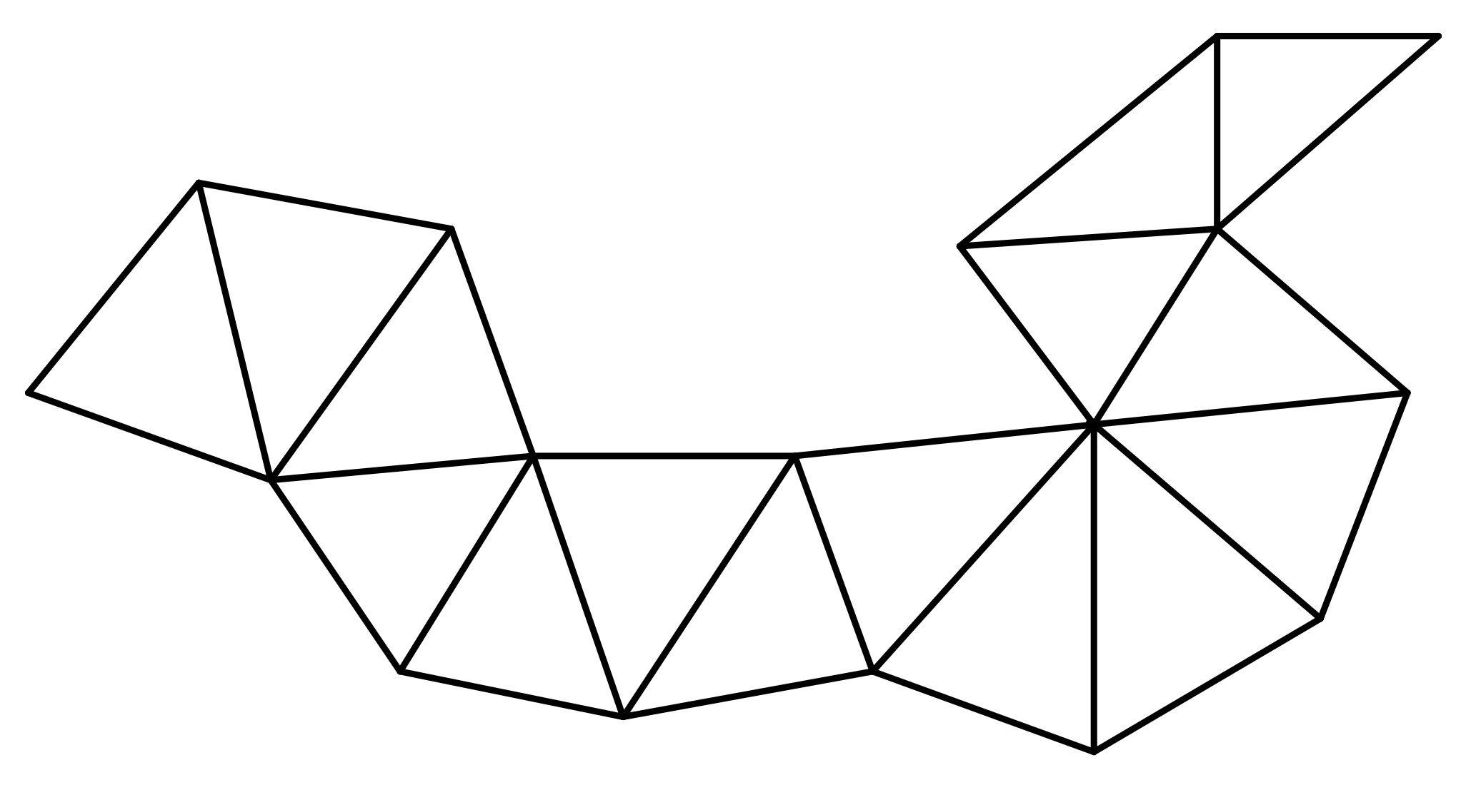
Figure 17: A triangle strip.

We want to make use of strips of triangles such as the one in figure 17. A triangle strip is a path in the graph that has

• the edges of $\hat{\Gamma}$ as vertices, and

• an edge for each pair of edges of $\hat{\Gamma}$ that are part of a common triangle.

We do not directly refer to the (abstract) edges and vertices of such a path, but talk instead only of (the original) triangles and edges. We assume in particular that:

• a triangle strip contains at least one edge, and

• repeated triangles or edges are allowed.

Lemma 8.

Given

• a triangle strip with vertex set $V$ and edge set $E$, and

• a extended monopole configuration $m$ with support contained in $V$,

there exists a extended flux configuration $\phi$ such that

$$\hat{\partial}\phi=m,\qquad\phi\subseteq E.$$ (71)

• Sketch of proof.Lets proceed by induction of the number of triangles. The base case is a single edge, where the result can be checked directly. For the inductive step, consider a strip with $n$ triangles that is composed of (i) a strip $s$ with $n-1$ triangles and (ii) an additional triangle $t$. Consider the vertex $v$ of $t$ that is not an endpoint of the last edge of $s$, and the edges $e_{1},e_{2}$ of $t$ meeting at $v$. The monopole $m(v)$ can take one of four values, each corresponding to a subset $\phi_{0}\subseteq\{e_{1},e_{2}\}$ via

  $$(\partial\phi_{0})(v)=m(v).$$ (72)

  Trivially

  $$m^{\prime}:=m+\partial\phi_{0}$$ (73)

  is a extended monopole configuration with support in $s$. By induction there exists $\phi_{1}$ with its edges in $s$ and such that $\partial\phi_{1}=m^{\prime}$, and thus it suffices to take $\phi=\phi_{0}+\phi_{1}$. ∎

A subset of colex faces $F$ is simple respect to a set of cells $C$ if, for every cell $c\in C$, the set of points of $c$ that also belong to some element of $F$ is simply connected.

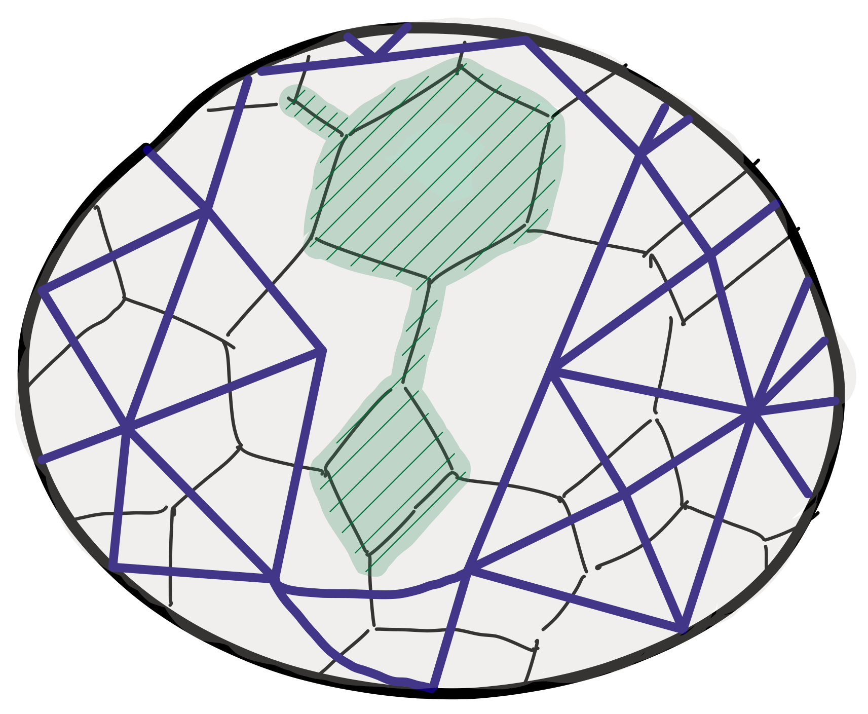
Figure 18: A cell $c$ of a 3-colex. The intersection of $c$ with some set of faces $F$ is indicated in green. The intersection is simply connected and thus compatible with $F$ being simple respect to a set of cells including $c$. The purple edges compose the graph $\gamma$ used in the proof of lemma 9.

Lemma 9.

Let $C$ be a set of cells and $F$ a set of colex faces that is simple respect to $C$. Let $E_{0}$ be the set of edges of $\hat{\Gamma}$ that are not dual to faces of $F$. For any path $p$ in $\hat{\Gamma}$ with

• all vertices dual to cells in $C$ except possibly the endpoints, and

• edge set $E_{p}$ such that

$$\emptyset\neq E_{p}\subseteq E_{0},$$ (74)

there exists a triangle strip with edge set $E$ such that

$$E_{p}\subseteq E\subseteq E_{0},\qquad|E|\leq 1+2(k_{\text{face}}-1)(|E_{p}|-1),$$ (75)

• Sketch of proof.It suffices to consider the case with $|E_{p}|=2$, since the shorter case is trivial and for longer paths we can concatenate the strips obtained for each pair of contiguous edges. Then $E_{p}=\{e,e^{\prime}\}$ with $e$ and $e^{\prime}$ meeting at a vertex $v$ that is dual to a cell $c\in C$. The surface of $c$ is a 2-colex and we can consider its dual graph, which has a vertex per face of $c$, and an edge per edge of $c$. Let $\gamma$ be the subgraph formed by

  • the vertices dual to faces not in $F$, and

  • the edges dual to edges not part of faces in $F$.

  This construction is illustrated in figure 18. By assumption, $\gamma$ is connected. Moreover,

  • the vertices in $\gamma$ are in one-to-one correspondence to the edges of $E_{0}$ with an endpoint at $v$, and

  • the edges of $\gamma$ are in one-to-one correspondence to the triangles of $\Gamma$ containing $v$ and with all their edges in $E_{0}$.

  Thus there is a path in $\gamma$ of length at most $k_{\text{face}}-1$ (since it visits each face of $c$ at most once) that provides the desired triangle strip from $e$ to $e^{\prime}$. The strip has at most $2k_{\text{face}}-3$ edges that are not in the path $p$. ∎

D.4 Closure

Here we make use of the various definitions of section VI. Below we identify the graphs $\Gamma_{i}$ and $\overline{\Gamma_{i}}$ with their sets of edges for convenience.

$\mathcal{O}_{i}$ is the set of flux configurations $\phi\subseteq\Phi_{i}$ such that the support of $\partial\phi$ is contained in the vertex set of $\overline{\Gamma_{i}}$.

Lemma 10.

Given some $i$, if

• $\Phi_{i}$ is simple respect to the set of cells complementary to $C_{i}$, and

• for any vertices $v,v^{\prime}$ of $\Gamma_{i}$ and any color $\kappa$

  $$d(v,v^{\prime})\leq k\,\overline{d}(v,v^{\prime}),$$ (76)

  $$\min\left(d_{\kappa}(v),d(v)\right)\leq k\,\overline{d_{\kappa}}(v),$$ (77)

then for any $\phi\in\mathcal{O}_{i}$ there exists $\phi^{\prime}\subseteq\overline{\Gamma_{i}}$ such that

$$\partial\phi=\partial\phi^{\prime},\qquad|\phi^{\prime}|\leq 4k(k_{\text{face}}-1)|\phi|.$$ (78)

• Sketch of proof.Regard such $\phi$ as a subgraph of the extended dual graph $\hat{\Gamma}$. We assume that $\phi$ is connected (because if it has several connected components $\phi_{j}$, it suffices to add the corresponding $\phi_{j}^{\prime}$) and that $\partial\phi\neq 0$ (because the case $\partial\phi=0$ is trivial, $\phi^{\prime}=\emptyset$).

  Let $V_{\phi}$ be the support of $\hat{\partial}\phi$. Choose a set $V$ containing the inner vertices of $V_{\phi}$ together with:

  • two outer vertices of $V_{\phi}$ of different colors, if $V_{\phi}$ contains outer vertices of at least two colors,

  • an outer vertex of $V_{\phi}$, if $V_{\phi}$ contains outer vertices of a single color,

  • no other vertices, otherwise.

  Choose some tree $t$ that is a subgraph of $\phi$ and has $V$ as its set of leafs (it exists: take any maximal tree of $\phi$ and remove any unwanted leafs repeatedly). By the construction suggested in the figure below (the red dots mark the outer vertices), there exists a collection of paths $p_{j}$, $j=1,\dots,n$ with edge sets $E_{j}$ such that

  • every $p_{j}$ has vertices of $V$ as endpoints,

  • the last vertex of $p_{j}$ is the first vertex of $p_{j+1}$,

  • only the first vertex of $p_{1}$ and the last of $p_{n}$ can be outer vertices, and

  • identifying the tree $t$ with its set of edges:

  $$t=\bigcup_{j}E_{j},\qquad\sum_{j}|E_{j}|\leq 2|t|$$ (79)

  For each $p_{j}$ we choose some path $p_{j}^{\prime}$ in $\hat{\Gamma}$ with edge set $E_{j}^{\prime}\subseteq\overline{\Gamma_{i}}$ such that

  $$|E_{j}^{\prime}|\leq k|E_{j}|$$ (80)

  and, on a case by case basis:

  • If the endpoints of $p_{j}$ are both inner vertices, then $p_{j}^{\prime}$ has the same endpoints as $p_{j}$.

  • If the endpoints of $p_{j}$ are an inner vertex $v$ and a $\kappa$-colored outer vertex, $p_{j}^{\prime}$ is either

    • a path connecting $v$ to a $\kappa$-colored outer vertex, or

    • the composition of two paths, each connecting $v$ to an outer vertex, with the colors of these two outer vertices different.

  Since $E_{j}\subseteq\Gamma_{i}$ and the inner vertices of $V$ are vertices of $\overline{\Gamma_{i}}$, such paths exist by assumption. Choose a triangle strip $s_{j}$ for each $p_{j}^{\prime}$ according to lemma 9. The set of edges

  $$E:=\bigcup_{j}E_{j}^{\prime}$$ (81)

  is clearly connected, and therefore there exists a triangle strip $s$ such that its triangle set is the union of the triangle sets of the strips $s_{j}$. Its set of edges $S$ satisfies

  $$|S| \leq 2(k_{\text{face}}-1)|E|\leq 2k(k_{\text{face}}-1)\sum_{j}|p_{j}|$$

  $$\leq 4k(k_{\text{face}}-1)|\phi|.$$ (82)

  Noting that for any two different colors $\kappa,\kappa^{\prime}$

  $$M=M_{\kappa}M_{\kappa^{\prime}},$$ (83)

  it is easy to check (case by case, according to the different possibilities considered above), that there exists a extended monopole configuration $m$ with no support outside the endpoints of the paths $p_{j}^{\prime}$ and such that its restriction to the inner vertices is $\partial\phi$. The result follows applying lemma 8. ∎

D.5 Boundary conditions

Clearly the set $\mathcal{C}_{i}$ defined in 15 always satisfies

$$\mathcal{C}_{i}\subseteq\mathcal{O}_{i}.$$ (84)

Therefore, lemma 2 follows from lemma 10. In fact, when lemma 10 holds, $\mathcal{C}_{i}$ takes the form

$$\mathcal{C}_{i}=\mathcal{O}_{i},$$ (85)

which corresponds to truly ‘open’ boundary conditions.

Appendix E Ball-local noise

This appendix discusses ball-local error distributions, introducing some results that are necessary for the analysis of JIT decoding in appendix F.

E.1 Locality and topological codes

The error correction threshold for a quantum error correcting code is often formulated in terms of local errors, see section III.4. Codes are often designed with the expectation that noise is indeed local or approximately so. The aim is for codes to have a high distance, defined as the smallest number of qubits supporting a non-trivial logical operator.

In the case of topological codes another kind of distance enters the picture: a distance defined by the geometry of the code, which can be typically codified in a hypergraph: its edges represent qubits, and the support of any non-trivial logical operator has to connect some pair of vertices that are at least separated by some given distance $d$. That is, a non-trivial logical operator can never have support within a ball of radius strictly smaller than $d/2$. This suggests introducing ball-local distributions of errors, as defined in section VIII.6.

E.2 From local to ball-local

The purpose of this section is to establish a result that is used in section F.2 to show that JIT error correction gives rise to ball-local noise.

Throughout this section it is assumed that some graph is given. We say that $v$ is a vertex of an edge set $E$ if $v$ is the endpoint of any edge in $E$.

A ball is a pair $(v,r)$ with $v$ a vertex, the center of the ball, and $r>0$ an integer, the radius of the ball. Such a ball is identified with the set of edges of the subgraph induced by the set of vertices that are at a distance at most $r$ from $v$. The radius of a ball $b$ is $\text{r}(b)$ and the sum of the radii of a set of balls $B$ is $\text{r}(B)$.

Lemma 11.

Let $\alpha>0$, $c\geq 1$ and $0\leq p\leq 1$. If

• the number of connected subsets of $n$ edges and with a given vertex, is bounded by $\alpha^{n}$,

• the edge set $\omega$ is a random variable satisfying, for any edge set $E$

  $$\text{prob}(E\subseteq\omega)\leq p^{|E|},$$ (86)

• the finite set $K$ of connected sets of edges is a function of $\omega$, and for any $\kappa\in K$

  $$|\kappa|\leq c|\kappa\cap\omega|,$$ (87)

then there exist, for each $\omega$, a ball set $W$, with

$$\bigcup K\subseteq\bigcup W,$$ (88)

and such that given any ball set $B$

$$\text{prob}\left(B\subseteq W\right)\leq\left(\frac{p}{p_{0}}\right)^{\text{r}(B)/2c},\qquad p_{0}:=(2\alpha)^{-c}.$$ (89)

We need an auxiliary result.

Lemma 12.

Given a finite set $K$ of connected sets of edges there exist

• disjoint sets $\kappa_{i}\in K$, and

• for each $i$, a ball $b_{i}$ with center a vertex of $\kappa_{i}$,

such that

$$\text{r}(b_{i})=2|\kappa_{i}|,\qquad\bigcup K\subseteq\bigcup_{i}b_{i}.$$ (90)

• Sketch of proof.We proceed by induction on $|K|$. The base case $K=\emptyset$ is trivial. For the inductive step $|K|=n$, assume that the statement holds for any lower cardinality. Choose $\kappa\in K$ with maximal cardinality. The case $\kappa=\emptyset$ is trivial, so we assume that $\kappa$ is not empty. Let

  $$K^{\prime}:=\{\kappa^{\prime}\in K\,|\,\kappa\cap\kappa^{\prime}=\emptyset\}.$$ (91)

  Apply the inductive assumption to $K^{\prime}$ to obtain $\kappa_{i}\in K^{\prime}$ and balls $b_{i}$, $i=1,\dots,m-1$, with the said properties. Set $\kappa_{m}=\kappa$, and let $b_{m}$ be any ball with center a vertex of $\kappa_{m}$ and radius $2|\kappa_{m}|$. Clearly all the elements of $K-K^{\prime}$ are subsets of $b_{m}$, and $\kappa_{m}$ overlaps with no $\kappa_{i}$, $i<m$. ∎

• Sketch of proof of lemma 11.Given $\omega$, choose $W$ as per the prescription of lemma 12 applied to the corresponding set $K$. It suffices to show that, given some ball set $B$, the probability that $W$ is a superset of $B$ is bounded as indicated. Let $B=\{b_{i}\}$. By construction, such an event requires that there exists

  • a disjoint collection of sets $\omega_{i}\subseteq\omega$,

  • connected sets of edges $\kappa_{i}$, each with the center of $b_{i}$ a vertex and

  $$\omega_{i}=\kappa_{i}\cap\omega,\qquad\text{r}(b_{i})=2|\kappa_{i}|,\qquad c|\omega_{i}|\geq|\kappa_{i}|.$$ (92)

  Consider the subset of $\omega$

  $$\omega^{\prime}=\bigsqcup_{i}\omega_{i},$$ (93)

  and notice that

  $$|\omega^{\prime}|=\sum_{i}|\omega_{i}|\geq\sum_{i}\frac{|\kappa_{i}|}{c}=\frac{\text{r}(B)}{2c}.$$ (94)

  For each ball $b_{i}$ there are at most $\alpha^{\text{r}(b_{i})/2}$ different $\kappa_{i}$ (compatible with $b_{i}$), and at most $2^{|\kappa_{i}|}=2^{\text{r}(b_{i})/2}$ possible subsets $\omega_{i}\subseteq\kappa_{i}$ for each such $\kappa_{i}$. This gives in total at most $(2\alpha)^{\text{r}(B)/2}$ possible $\omega^{\prime}$ that can contribute to the event $B\subseteq W$. Each contributes a probability

  $$\text{prob}(\omega^{\prime}\subseteq\omega)\leq p^{|\omega^{\prime}|}\leq p^{\text{r}(B)/2c}.\qed$$ (95)

E.3 Ball aggregation

The following results quantifies how unlikely large connected clusters of balls are. The settings are as in section E.2.

Lemma 13.

Let $\alpha>0$, $c\geq 1$ and $0\leq p\leq 1$. If

• the number of self-avoiding walks (SAW) of length at most $n$ and starting point on any given vertex is bounded by $\alpha^{n}$,

• the ball set $W$ is a random variable satisfying, for any ball set $B$

  $$\text{prob}(B\subseteq W)\leq p^{\text{r}(B)},$$ (96)

• the edge sets $E_{i}$ are the connected components of $\bigcup W$.

Then there exist, for each $W$, balls $b_{i}$ such that

$$E_{i}\subseteq b_{i},$$ (97)

and the set $A:=\{b_{i}\}$ is a random variable satisfying for any ball set $B$

$$\text{prob}\left(B\subseteq A\right)\leq\left(\frac{p}{p_{0}}\right)^{\text{r}(B)/2},\qquad p_{0}:=\left(\frac{2}{3e\alpha}\right)^{2}.$$ (98)

• Sketch of proof.For each $W$ and each $i$, let $W_{i}\subseteq W$ be the subsets forming the unique partition of $W$ such that

  $$\bigcup W_{i}=E_{i}.$$ (99)

  We choose $b_{i}$ as follows. Consider any two vertices $v,v^{\prime}$ of $E_{i}$ with distance equal to the diameter of $E_{i}$. It is not difficult to check that there exists

  • a SAW $q$ from $v$ to $v^{\prime}$, and

  • a ball subset $V\subseteq W_{i}$ such that $q$ visits all the the centers of the balls in $V$ and has length

    $$|q|\leq 2\text{r}(V).$$ (100)

  We set $b_{i}=(v,2\text{r}(V))$.

  The relation (97) is satisfied because by (100) the diameter of $E_{i}$ is bounded by $2\text{r}(V)$. As for (98), given any ball set $B$, the condition $B\subseteq A$ implies that for each ball $b\in B$ there exists such a SAW $q$ and ball set $V\subseteq W$, and these ball sets are mutually disjoint for different elements of $B$. By construction

  $$\text{prob}\left(V\subseteq W\right)\leq p^{\text{r}(V)}=p^{\text{r}(b)/2}$$ (101)

  and thus

  $$\text{prob}\left(B\subseteq A\right)\leq p^{\text{r}(B)/2}\prod_{b\in B}f\left(\frac{\text{r}(b)}{2},\text{r}(b)\right)$$ (102)

  where $f(r,l)$ is the maximal number of pairs $(q,V)$ with $V$ a ball set with $\text{r}(V)=r$ and $q$ a SAW that visits the center of each ball in $V$, has length $|q|\leq l$ and has a fixed starting point (the argument of the maximization). For a fixed $q$, the number of possible sets $V$ is bounded by the number of configurations of $r$ identical particles on $l+1$ ‘states’, which equals the number of binary strings with length $r+l$ and weight $l$. That is, we have

  $$f(r,l)\leq\alpha^{l}\binom{r+l}{l}$$ (103)

  and the result follows using the bound

  $$\binom{a}{b}<\left(\frac{ae}{b}\right)^{b}.\qed$$ (104)

E.4 Threshold for $\mathbf{Z}_{2}$ charge error correction

The purpose of this section is to show that a well-known class of efficient decoders exhibits an error correction threshold for ball-local noise.

E.4.1 Decoding a $\mathbf{Z}_{2}$ charge

The decoding problem of a single $\mathbf{Z}_{2}$ charge Dennis et al. (2002) is as follows:

• a (syndrome) graph represents the code structure,

• an error is represented by a subset of edges $E$,

• there are inner vertices that represent a check operator, and outer vertices that do not,

• the syndrome $\partial E$ of an error is represented by a set of inner vertices, those that are the endpoint of an odd number of edges in the error set.

A decoder outputs a set of edges $E^{\prime}$ compatible with the error syndrome, i.e. such that $\partial E^{\prime}=\partial E$. The original error $E$ and the decoded error $E^{\prime}$ can be combined into a logical error $E+E^{\prime}$ (an error with trivial syndrome). Decoding fails when $E+E^{\prime}$ is non-trivial, i.e. affects the encoded information.

Minimum-weight decoders output a set $E^{\prime}$ with minimum cardinality among those compatible with the syndrome. There exist efficient implementations Dennis et al. (2002).

E.4.2 Threshold for ball-local noise

The next argument shows that minimum-weight decoding of a $\mathbf{Z}_{2}$ charge exhibits an error threshold for ball-local noise. Assume that a family of codes is labeled with an integer $d$ that can be arbitrarily large, so that:

• the number of self-avoiding walks (SAW) of length at most $n$ and starting point on any given vertex is bounded by $\alpha^{n}$,

• the number of vertices is polynomial in $d$,

• every non-trivial logical error connects two outer vertices with distance at least $d$.

We denote by $|p|$ the length of a path $p$. The argument is divided in steps.

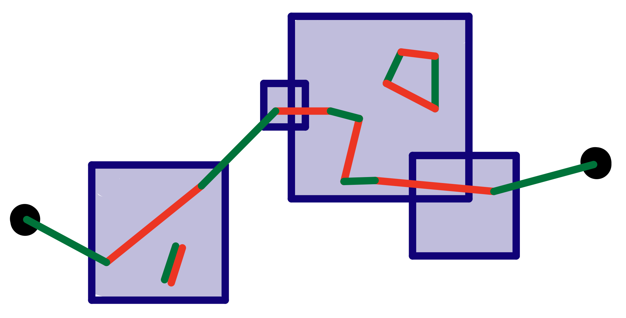
Figure 19: The original error $E$ (red) and the estimated error $E^{\prime}$ (green) connect two outer vertices (black dots) in the event of a failure. The purple regions represent the balls in the set $W$.

0. In the event of failure $E+E^{\prime}$ connects two outer vertices $v$ and $v^{\prime}$ with distance at least $d$. The error $E$ is a subset of $\bigcup W$, with $W$ as in $\eqref{eq:ball-local}$. This is illustrated in figure 19.

1. It is not difficult to show that there exist ball sets $B_{i}$, $i=1,\dots,n$, and a SAW $w$ from $v$ to $v^{\prime}$ obtained by concatenating together a sequence of paths

$$(w_{0},w_{1}^{\prime},w_{1},\cdots,w_{n}^{\prime},w_{n}),$$ (105)

such that

• $B_{i}\cap B_{j}=\emptyset$ for $i\neq j$,

• $w_{i}$ has its edges in $E^{\prime}$,

• $w_{j}^{\prime}$ visits the center of each ball of $B_{j}$, and

  $$|w^{\prime}_{j}|\leq 2r(B_{j}).$$ (106)

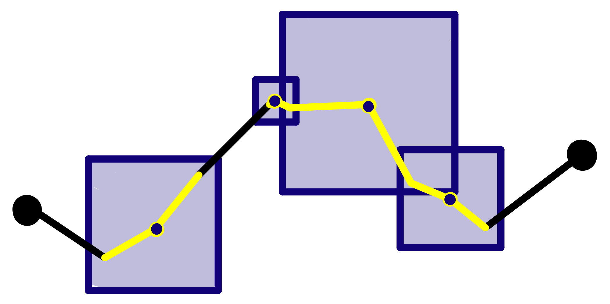
Figure 20: A path as in equation (105), with the paths $w_{i}$ in black and the paths $w_{i}^{\prime}$ in yellow.

2. Let $L$ be the set of edges of $w$. Since the endpoints of $w$ are outer vertices

$$\partial(E^{\prime}+L)=\partial E^{\prime},$$ (107)

so that by the minimality of $|E^{\prime}|$, and noting that by construction $L-E^{\prime}$ only contains edges of the paths $w_{i}^{\prime}$,

$$\sum_{j=1}^{n}|w_{j}^{\prime}|\geq|L-E^{\prime}|\geq|L\cap E^{\prime}|\geq\sum_{i=0}^{n}|w_{i}|,$$ (108)

which yields

$$|w|\leq 4r(B),\qquad B:=\bigsqcup_{j}B_{j}.$$ (109)

3. We have found that a failure event requires of the existence of a SAW $w$ and a set of balls $B\subseteq W$ such that $w$ visits the centers of all the balls in $B$ and

$$d\leq|w|\leq 4r(B).$$ (110)

The probability of such an event for a fixed set of balls $B$ is bounded by $p^{r(B)}$, and thus the same is true if we fix both $w$ and $B$. The number of such pairs $w$ and $b$ given a fixed starting point for $w$ is bounded by $f(\text{r}(B),4\text{r}(B))$ with $f$ as in (103). With this observation, the rest of the argument is standard Dennis et al. (2002).

Appendix F The cost of naivety

The aim of this appendix is to show that the residual noise $\hat{\omega}$ of the naive decoder, as described in equation 47, follows a ball-local distribution under reasonable conditions, given that the error rate of the noise afflicting ancilla qubits is below a threshold.

F.1 Technical conditions on the decoders

It is is unclear if minimum weight errors can be computed efficiently for tetrahedral codes. However, as discussed in Bombin (2015b), it is possible to relax the minimization condition in such a way that efficient decoders exist and certain proof techniques of the minimum weight case can be extended.

The relaxed conditions, adapted to the present scenario, are as follows. There exists $k_{\text{min}}$ such that for every code in the family of tetrahedral color codes of interest and every step $i$ of JIT error correction the open/closed boundary conditions decoders satisfy:

Minimization conditions

• For any $\omega\subseteq\Phi_{i}$ and any connected component $\kappa$ of $D_{i}(\omega)\cup\omega$

  $$|\kappa|\leq k_{\text{min}}|\kappa\cap\omega|.$$ (111)

• For any $\omega\subseteq\overline{\Phi_{i}}$ and any connected component $\kappa$ of $D_{i}^{\prime}(\omega)\cup\omega$

  $$|\kappa|\leq k_{\text{min}}|\kappa\cap\omega|.$$ (112)

The notion of connectedness here is given by the dual graph $\Gamma$ of the 3-colex. The key relationship between connectedness and syndrome is that if $\gamma$ has trivial syndrome, then every connected component of $\gamma$ has trivial syndrome too. Notice that for decoders that compute minimum weight errors

$$k_{\text{min}}=2.$$ (113)

F.2 Ball-locality of the syndrome

The key link between JIT error correction and ball-local noise is lemma 14 below. Together with lemma 11, it shows that indeed the residual noise of JIT decoding follows a ball-local distribution (under the given conditions). The notation here is as in section VIII.5.

Lemma 14.

If the minimization and closure conditions hold, there exists connected flux configurations $\kappa_{j}$ such that

$$\hat{\omega}\subseteq\bigcup_{j}\kappa_{j},\qquad|\kappa_{j}|\leq c|\kappa_{j}\cap\omega|,$$ (114)

where

$$c=2k_{\text{min}}(k_{\text{min}}k_{\text{close}}+1)+1.$$ (115)

• Proof.Consider the flux configurations

  $$\delta_{i}:=\omega_{i-1}^{\prime}+\omega^{\prime}_{i}\cap\Phi_{i-1},$$ (116)

  $$\Omega_{i}:=\epsilon_{i}\cup\omega_{i-1}^{\prime}\cup\omega_{i}^{\prime}\cup\omega,$$ (117)

  and the partition into connected components

  $$\Omega_{i}=\bigsqcup_{j}\kappa_{i}^{(j)}.$$ (118)

  Any connected component of $\delta_{i}$ is an element of $\mathcal{C}_{i-1}$ because $\delta_{i}\in\mathcal{C}_{i-1}$. Since $\delta_{i}\subseteq\Omega_{i}$ this implies

  $$\kappa_{i}^{(j)}\cap\delta_{i}\in\mathcal{C}_{i-1}.$$ (119)

  Thus by the closure condition there exist

  $$\mu_{i}^{(j)}\in\overline{\Phi}_{i-1}$$ (120)

  with

  $$\mu_{i}^{(j)}+(\kappa_{i}^{(j)}\cap\delta_{i})\in\mathcal{C},\qquad|\mu_{i}^{(j)}|\leq k_{\text{close}}|\kappa_{i}^{(j)}\cap\delta_{i}|.$$ (121)

  We assume that each connected component of $\mu_{i}^{(j)}$ is connected to $(\kappa_{i}^{(j)}\cap\delta_{i})$, as such a choice is trivially always possible. We perform another partition in connected components, namely

  $$\mu_{i}\cup\Omega_{i}=\bigsqcup_{J}\bar{\kappa}_{i}^{(J)},\qquad\mu_{i}:=\sum_{j}\mu_{i}^{(j)}.$$ (122)

  where the indices $J$ form a partition of the set of indices of the partition $\eqref{partition}$:

  $$\bar{\kappa}_{i}^{(J)}\cap\Omega_{i} =\bigsqcup_{j\in J}\kappa_{i}^{(j)},$$ (123)

  $$\bar{\kappa}_{i}^{(J)}\cap\mu_{i} =\bigsqcup_{j\in J}\mu_{i}^{(j)}.$$ (124)

  The bound in $\eqref{bound_closure}$ translates into

  $$|\bar{\kappa}_{i}^{(J)}\cap\mu_{i}|\leq k_{\text{close}}|\bar{\kappa}_{i}^{(J)}\cap\delta_{i}|\leq k_{\text{close}}|\bar{\kappa}_{i}^{(J)}\cap(\omega_{i-1}^{\prime}\cup\omega_{i}^{\prime})|.$$ (125)

  Since

  $$\delta_{i}+\mu_{i}\in\mathcal{C},$$ (126)

  we have, using (44),

  $$\epsilon_{i}=\delta_{i}+\overline{D_{i-1}}(\delta_{i})=\mu_{i}+D_{i-1}^{\prime}(\mu_{i}),$$ (127)

  and thus the minimization condition on $D_{i-1}^{\prime}$ yields

  $$|\bar{\kappa}_{i}^{(J)}\cap(\epsilon_{i}\cup\mu_{i})|\leq k_{\text{min}}|\bar{\kappa}_{i}^{(J)}\cap\mu_{i}|.$$ (128)

  Since, for any $i$,

  $$\omega^{\prime}_{i}=\omega\cap\Phi_{i}+D_{i}(\omega\cap\Phi_{i}),$$ (129)

  the minimazation condition on $D_{i}$ and $D_{i-1}$ yields

  $$|\bar{\kappa}_{i}^{(J)}\cap(\omega_{i-1}^{\prime}\cup\omega_{i}^{\prime})|\leq 2k_{\text{min}}|\bar{\kappa}_{i}^{(J)}\cap\omega|.$$ (130)

  Putting together $(\ref{bound_closure_2},\ref{bound_min_1},\ref{bound_min_2})$,

  $$|\bar{\kappa}_{i}^{(J)}| \leq|\bar{\kappa}_{i}^{(J)}(\epsilon_{i}\cup\mu_{i})|+|\bar{\kappa}_{i}^{(J)}\cap(\omega_{i}^{\prime}\cup\omega_{i})|+|\bar{\kappa}_{i}^{(J)}\cap\omega|$$

  $$\leq c|\bar{\kappa}_{i}^{(J)}\cap\omega|,$$ (131)

  which is enough because, by $\eqref{eq:JIT_error}$,

  $$\hat{\omega}\subseteq\bigcup_{i}\bigcup_{J}\bar{\kappa}_{i}^{(J)}.\qed$$ (132)

F.3 Technical conditions on the lattice

Theorem 15 below relies on the colexes satisfying a set of conditions that ensure that the local structure of the colexes is sufficiently uniform. When the object of interest is not a single tetrahedral code, but rather a family of such encodings (e.g. in the study of error thresholds), this uniformity condition should be satisfied by the whole family of colexes.

Let $\mathcal{B}$ denote the set of all balls in the dual graph $\Gamma$ of a tetrahedral colex, and $\mathcal{B}^{\prime}$ the set of all balls in its $X$-error syndrome hypergraph. The edges of this hypergraph are the physical qubits of the code. Thus, every ball in $\mathcal{B}^{\prime}$ can be identified with its set of qubits.

Uniformity conditions

• The number of connected subgraphs of the dual graph $\Gamma$ with $n$ edges and containing any given vertex is bounded by $\alpha^{n}$.

• There are constants $m_{0},m_{1}$ and a map

  $$\mathcal{M}:\mathcal{B}\longrightarrow\mathcal{B}^{\prime}$$ (133)

  such that

  • the preimage of any ball in $\mathcal{B}^{\prime}$ under $\mathcal{M}$ has at most $m_{0}$ elements,

  • the radius of $\mathcal{M}(b)$ is $m_{1}\text{r}(b)$, and

  • for any ball $b\in\mathcal{B}$ and any syndrome $\phi\subseteq b$ there exists $x\in P_{X}$ with syndrome $\phi$ and support a subset of $\mathcal{M}(b)$.

These conditions are satisfied for families of tetrahedral colexes with a uniform and flat local structure, including at facets and corners, such as the one discussed in Bombin (2015a). The first condition trivially holds if the vertices of the dual graph $\Gamma$ have bounded valence. The validity of the second is rooted in the homological structure of the codes, as can be verified using the mapping in Kubica et al. (2015).

F.4 Residual noise

The notation here is as in section VIII.5.

Theorem 15.

If the closure, minimization and uniformity conditions hold, and the flux configuration $\omega$ follows a local distribution with rate $p\leq p_{0}$, with, for $c$ as in (115),

$$p_{0}=\left(\frac{8}{(3em_{0})^{4}\alpha^{5}}\right)^{c},$$ (134)

then there exists for each $\omega$ some $x\in P_{X}$ with syndrome $\hat{\omega}$ such that $x$ follows a ball-local distribution with rate

$$\left(\frac{p}{p_{0}}\right)^{1/4m_{1}c}.$$ (135)

• Proof.By lemmas 14, 11 and 13 there exists for each $\omega$ a set of balls

  $$A=\{b_{i}\}$$ (136)

  and a partition

  $$\hat{\omega}=\bigsqcup_{i}\hat{\omega}_{i}$$ (137)

  such that

  $$\hat{\omega}_{i}\subseteq b_{i},$$ (138)

  the sets of edges $\hat{\omega}_{i}$ are mutually disconnected, and

  $$\text{prob}(B\subseteq A)\leq\left(\frac{p}{p_{0}^{\prime}}\right)^{\text{r}(B)/4c},\qquad p_{0}^{\prime}=\left(\frac{8}{(3e)^{4}\alpha^{5}}\right)^{c}$$ (139)

  Since $\hat{\omega}$ is a syndrome so is each $\hat{\omega}_{i}$, and thus there exists $x\in P_{X}$ with syndrome $\hat{\omega}$ and support on a subset of the qubits in the balls of $A^{\prime}=\mathcal{M}[A]$, the image of $A$ under $\mathcal{M}$. Each $B^{\prime}\subseteq\mathcal{B}^{\prime}$ defines a set $m(B^{\prime})$ containing those ball sets $B\subseteq\mathcal{B}^{\prime}$ such that

  • $\mathcal{M}[B]=B^{\prime}$, and

  • for any $b,b^{\prime}\in B$ such that $b\neq b^{\prime}$, $\mathcal{M}(b)\neq\mathcal{M}(b^{\prime})$.

  The result follows observing that

  $$|m(B^{\prime})|\leq m_{0}^{|B^{\prime}|}\leq m_{0}^{\text{r}(B^{\prime})/m_{1}}$$ (140)

  and

  $$\text{prob}(B^{\prime}\subseteq A^{\prime})\leq\sum_{B\in m(B^{\prime})}\text{prob}(B\subseteq A).\qed$$ (141)

References

- Brown et al. (2016a) B. Brown, D. Loss, J. Pachos, C. Self, and J. Wootton, Reviews of Modern Physics 88, 045005 (2016a).
- Lidar and Brun (editors) D. Lidar and T. Brun (editors), Quantum Error Correction (Cambridge University Press, New York, 2013).
- Campbell et al. (2017) E. Campbell, B. Terhal, and C. Vuillot, Nature 549, 172 (2017).
- Bravyi and Kitaev (2005) S. Bravyi and A. Kitaev, Phys. Rev. A 71, 22316 (2005).
- Bombin (2016) H. Bombin, New J. Phys. 18, 043038 (2016).
- Raussendorf and Briegel (2001) R. Raussendorf and H. J. Briegel, Physical Review Letters 86, 5188 (2001).
- Rudolph (2017) T. Rudolph, APL Photonics 2, 030901 (2017).
- Kitaev (1997) A. Kitaev, Russ. Math. Surv. 52, 1191 (1997).
- Gottesman (1996) D. Gottesman, Phys. Rev. A 54, 1862 (1996).
- Dennis et al. (2002) E. Dennis, A. Kitaev, A. Landahl, and J. Preskill, J. Math. Phys. 43, 4452 (2002).
- Bombin (2013) H. Bombin, in Quantum Error Correction, edited by D. Lidar and T. Brun (Cambridge University Press, New York, 2013).
- Raussendorf et al. (2007) R. Raussendorf, J. Harrington, and K. Goyal, New J. Phys. 9, 199 (2007).
- Bombin and Martin-Delgado (2009) H. Bombin and M. Martin-Delgado, J. Phys. A: Math. and Theor. 42, 95302 (2009).
- Bombin (2010) H. Bombin, Phys. Rev. Lett. 105, 30403 (2010).
- Horsman et al. (2012) C. Horsman, A. Fowler, S. Devitt, and R. Van Meter, New J. Phys. 14, 123011 (2012).
- Landahl and Ryan-Anderson (2014) A. Landahl and C. Ryan-Anderson, arXiv preprint arXiv:1407.5103 (2014).
- Yoder and Kim (2017) T. Yoder and I. Kim, Quantum 1, 2 (2017).
- Bravyi and König (2013) S. Bravyi and R. König, Phys. Rev. Lett. 110, 170503 (2013).
- Bombin et al. (2013) H. Bombin, R. W. Chhajlany, M. Horodecki, and M. Martin-Delgado, New J. Phys. 15, 55023 (2013).
- Bombin and Martin-Delgado (2006) H. Bombin and M. Martin-Delgado, Phys. Rev. Lett. 97, 180501 (2006).
- Bombin and Martin-Delgado (2007) H. Bombin and M. Martin-Delgado, Phys. Rev. Lett. 98, 160502 (2007).
- Bombin (2015a) H. Bombin, New J. Phys. 17, 083002 (2015a).
- (23) H. Bombin, “Local gates in 3d topological codes,” ArXiv: quant-ph/1810.?????
- Bombin (2015b) H. Bombin, Phys. Rev. X 5, 031043 (2015b).
- Campbell (2018) E. Campbell, arXiv preprint arXiv:1805.09271 (2018).
- Raussendorf et al. (2005) R. Raussendorf, S. Bravyi, and J. Harrington, Physical Review A 71, 062313 (2005).
- Raussendorf et al. (2006) R. Raussendorf, H. J., and G. K., Ann. Phys. 321, 2242 (2006).
- Raussendorf and Harrington (2007) R. Raussendorf and J. Harrington, Physical review letters 98, 190504 (2007).
- Knill et al. (1996) E. Knill, R. Laflamme, and W. Zurek, arXiv: quant-ph/9610011 (1996).
- Eastin and Knill (2009) B. Eastin and E. Knill, Phys. Rev. Lett. 102, 110502 (2009).
- Bravyi and Cross (2015) S. Bravyi and A. Cross, arXiv:1509.03239 (2015).
- Jochym-O’Connor and Bartlett (2015) T. Jochym-O’Connor and S. D. Bartlett, arXiv:1509.04255 (2015).
- Calderbank and Shor (1996) A. Calderbank and P. W. Shor, Phys. Rev. A 54, 1098 (1996).
- Steane (1996) A. Steane, Proc. R. Soc. London, Ser. A 452, 2551 (1996).
- Gross and Eisert (2007) D. Gross and J. Eisert, Physical review letters 98, 220503 (2007).
- Chen et al. (2010) X. Chen, Z.-C. Gu, and X.-G. Wen, Physical review b 82, 155138 (2010).
- Gottesman and Chuang (1999) D. Gottesman and I. Chuang, Nature 402, 390 (1999).
- Duclos-Cianci and Poulin (2010) G. Duclos-Cianci and D. Poulin, Phys. Rev. Lett. 104, 50504 (2010).
- Sarvepalli and Raussendorf (2012) P. Sarvepalli and R. Raussendorf, Physical Review A 85, 022317 (2012).
- Duclos-Cianci and Poulin (2013) G. Duclos-Cianci and D. Poulin, arXiv preprint arXiv:1304.6100 (2013).
- Herold et al. (2015) M. Herold, E. Campbell, J. Eisert, and M. Kastoryano, npj Quantum Information 1, 15010 (2015).
- Herold et al. (2017) M. Herold, M. Kastoryano, E. Campbell, and J. Eisert, New Journal of Physics 19, 063012 (2017).
- Dauphinais and Poulin (2017) G. Dauphinais and D. Poulin, Communications in Mathematical Physics 355, 519 (2017).
- Kubica and Preskill (2010) A. Kubica and J. Preskill, arXiv:1002.4930 (2010).
- Kubica et al. (2015) A. Kubica, B. Yoshida, and F. Pastawski, New Journal of Physics 17, 083026 (2015).
- Kubica et al. (2018) A. Kubica, M. Beverland, F. Brandão, J. Preskill, and K. Svore, Physical review letters 120, 180501 (2018).
- Brown et al. (2016b) B. Brown, N. Nickerson, and D. Browne, Nat. Comm. 7, 12302 (2016b).
- Bolt et al. (2016) A. Bolt, G. Duclos-Cianci, D. Poulin, and T. Stace, Physical review letters 117, 070501 (2016).
- (49) N. Nickerson and H. Bombin, “Measurement based fault tolerance beyond foliation,” ArXiv: quant-ph/1810.?????