Fast radio burst source properties from polarization measurements

Abstract

Recent polarization measurements of fast radio bursts (FRBs) provide new insights on these enigmatic sources. We show that the nearly 100% linear polarization and small variation of the polarization position angles (PAs) of multiple bursts from the same source suggest that the radiation is produced near the surface of a strongly magnetized neutron star. As the emitted radiation travels through the magnetosphere, the electric vector of the X-mode wave adiabatically rotates and stays perpendicular to the local magnetic field direction. The PA freezes at a radius where the plasma density becomes too small to be able to turn the electric vector. At the freeze-out radius, the electric field is perpendicular to the magnetic dipole moment of the neutron star projected in the plane of the sky, independent of the radiation mechanism or the orientation of the magnetic field in the emission region. We discuss a number of predictions of the model. The variation of PAs from repeating FRBs should follow the rotational period of the underlying neutron star (but the burst occurrence may not be periodic). Measuring this period will provide crucial support for the neutron star nature of the progenitors of FRBs. For FRB 121102, the small range of PA variation means that the magnetic inclination angle is less than about $20^{\rm o}$ and that the observer’s line of sight is outside the magnetic inclination cone. Other repeating FRBs may have a different range of PA variation from that of FRB 121102, depending on the magnetic inclination and the observer’s viewing angle.

1 Introduction

Fast radio bursts (FRBs) are millisecond-duration, bright, transient events, first detected at $\sim$GHz frequencies by the Parkes Telescope during pulsar surveys (Lorimer et al., 2007; Thornton et al., 2013). These bursts are distributed roughly isotropically in the sky, and have an all-sky rate of $\sim$$10^{3}$ to $10^{4}\rm\ day^{-1}$ above $\sim$$1\rm\ Jy\,ms$ fluence (Thornton et al., 2013; Keane & Petroff, 2015; Rane et al., 2016; Champion et al., 2016; Bhandari et al., 2018). One object (FRB 121102) has produced numerous bursts (Spitler et al., 2016; Scholz et al., 2016), and its sky location has been determined with an accuracy of $\sim$$0.1^{\prime\prime}$ by interferometry with the Jansky Very Large Array (Chatterjee et al., 2017). The source is found to be associated with a dwarf star-forming host galaxy at redshift z = 0.19273 (Tendulkar et al., 2017). The FRB is also associated with a persistent radio source (Chatterjee et al., 2017), and their projected separation is further pinned down to $\lesssim 0.01^{\prime\prime}$ ($\lesssim 40\rm\ pc$ in physical distance) by the European VLBI Network (Marcote et al., 2017).

The dispersion measure for FRBs, i.e. the number of free electrons per unit area between the source and the Earth, is between $\sim$200 and $2.5\times 10^{3}\,$cm^-3pc. For most of the reported bursts, this column density is larger than the contribution from the interstellar medium in the Milky Way by roughly an order of magnitude, which suggests that these events lie at a distance of a billion light years or more (see Katz, 2016, 2018, for recent reviews). This is confirmed by the host galaxy of the repeater FRB 121102, which is at $\sim$$1\,$Gpc. If the source radiates isotropically, then the energy release in the radio band for bursts from the repeater FRB 121102 varies from $\sim$$10^{37}$ to $10^{40}\,$erg (Spitler et al., 2016; Scholz et al., 2016; Law et al., 2017; Oostrum et al., 2017). For other FRBs with unknown distances, if the dispersion measure is dominated by the intergalactic medium, then the isotropic equivalent energy release in the radio band ranges from $\sim$$10^{39}$ to $10^{42}\,$erg (data from the FRB catalog).

Polarization properties of many of the (so-far) non-repeating FRBs have been measured (e.g. Petroff et al., 2015; Masui et al., 2015; Ravi et al., 2016; Petroff et al., 2017; Caleb et al., 2018), and the reported degree of linear polarization is between $\sim$0% and $\sim$80%. However, the frequency resolution of most surveys is limited (e.g., channel width of 0.4 MHz at 1.4 GHz), so the measurements could be affected by Faraday depolarization. Therefore, the above measurements of the degree of linear polarization should be viewed as lower limits. Polarization of the repeater (FRB 121102) was measured at 4-8 GHz with high accuracy for 26 bursts spread over 7 months in the rest frame of the host galaxy (Michilli et al., 2018; Gajjar et al., 2018). The degree of linear polarization for all these bursts was nearly 100%. Over the duration of each burst, the polarization position angle (PA), or the orientation of the electric field plane at frequency $\nu$$\rightarrow$$\infty$, stayed nearly constant. However, the PA was found to vary from burst to burst but within a small range. The (error-weighted) standard deviation for the PAs of the 26 bursts detected is $\sigma\approx 11.5^{\rm o}$, so we have a crude estimate of PA variation range to be $\pm\Delta{\rm PA}_{\rm max}\sim\pm 2\sigma\sim\pm 20^{\rm o}$. Moreover, the rotation measure (RM) was found to be about $10^{5}$ rad m^-2, which varied from one burst to another by about 10%. The contribution to the RM from the Milky Way galaxy and the intergalactic medium is estimated to be less than about 10² rad m^-2 (Michilli et al., 2018), so most of the RM is likely to be from the host galaxy and possibly the close vicinity of the burst; the magnetic field strength inferred from the RM is, therefore, of order milli-Gauss. The high degree of linear polarization and the small range of PA variations among different bursts over 7 months provide important constraints on the radiation mechanism and the FRB source properties, which we address in this paper.

2 Polarization angle change as waves move through a neutron star magnetosphere

The sub-millisecond variability of FRB lightcurves (e.g. $\sim$30$\,\mu$s for FRB170827, Farah et al., 2018) suggests that the underlying object is likely to be a neutron star or a stellar-mass black hole. Considering that the brightness temperature of FRB radiation is $\gtrsim$10${}^{35}\,$K (Katz, 2014; Luan & Goldreich, 2014), the radiation mechanism must be a coherent process where particles in the source radiate in phase. Broadly speaking, this means that the radiation mechanism is either a maser-type process (such as synchrotron, curvature, cyclotron-Cherenkov, or other plasma masers) or the antenna mechanism. Most maser and plasma processes require the wave frequency to be closely related to either the plasma frequency or the cyclotron frequency, and thus the source region should have a relatively low electron density (of order $10^{10}\gamma^{1/2}\,$cm^-3) and/or modest magnetic field strength of order 10${}^{3}\gamma\,$G (Lu & Kumar, 2018), where $\gamma$ is the typical Lorentz factor of the radiating particles. These conditions arise naturally far from the neutron star (or black hole), near or beyond the light cylinder radius, $R_{\rm L}=c/\Omega$, where $\Omega$ is the rotational angular frequency of the neutron star, and $c$ is the speed of light. The antenna mechanism, on the other hand, requires very strong magnetic field ($B\lower 2.0pt\hbox{$\,\buildrel\scriptstyle>\over{\scriptstyle\sim}\,$}10^{14}\,$G) and high electron density ($n\lower 2.0pt\hbox{$\,\buildrel\scriptstyle>\over{\scriptstyle\sim}\,$}10^{17}\,$cm^-3), which means that it can only operate within a distance of a few $R_{\rm ns}$ from the surface of the neutron star (Kumar et al., 2017), where $R_{\rm ns}$ is the neutron star radius.

The small PA variation between bursts from the repeater may require fine tuning for any mechanism that operates at large distances from the neutron star or black hole, because the magnetic field direction can change randomly in time and space (and hence from burst to burst). In this paper, we assume that FRBs are produced in the magnetosphere of neutron stars somewhere between the surface and the light cylinder, where the magnetic field configuration is likely to be stable (in the corotating frame of the neutron star) over a long period $\gtrsim$7 months. For models in which the bursts are generated near the surface, if the emitting region moves around randomly between bursts, and hence samples different local magnetic field configurations (which would generally be a superposition of dipole plus higher order multipoles and could, in principle, be arbitrarily complicated), it might seem that the PA should correspondingly change by a large amount between bursts. This turns out not to be the case.

We show that the PA of bursts generated near the neutron star surface is modified as the wave travels through the magnetosphere in such a way that the escaping radiation is nearly 100% linearly polarized, with the electric vector always perpendicular to the magnetic dipole moment projected in the plane of the sky. Thus, the PAs of different bursts are not expected to vary by much more than the angle between the rotation axis and magnetic axis of the neutron star (provided the observer is outside the magnetic inclination cone, see §3). This result does not depend on the radiation mechanism or the magnetic field direction at the source position.

In the following, we first describe the basic picture of radio waves propagating through a neutron star magnetosphere (§2.1) and then solve the linear wave equation for the change of PA along the propagation path (§2.2). Then in §2.3, we extend the discussion to the high intensity FRB waves in the non-linear regime and calculate the location beyond which the magnetosphere cannot supply sufficient current density and hence the PA freezes.

2.1 The Basic Picture

Consider an electromagnetic (EM) wave of frequency $\omega$ propagating in a quasi-static medium with magnetic field $B$ and plasma frequency $\omega_{p}$; $\omega_{p}^{2}=4\pi q^{2}\sum_{s}(n_{s}/m_{s})$, where $q$, $m_{s}$ and $n_{s}$ are the charge, mass and number density of electrons ($s=-$) and protons/positrons ($s=+$). The magnetosphere of a neutron star is usually not charge neutral everywhere, and hence $n_{+}\neq n_{-}$. It is convenient to express the two polarization states of EM radiation in the presence of a strong magnetic field (to be quantified shortly) as those with electric vector perpendicular to the plane of the magnetic and wave vectors (called the X-mode) and those with electric vector in this plane (the O-mode). The cyclotron frequency of electrons (or positrons) is $\omega_{B}=qB/(mc)$ and the medium of interest to us has a strong magnetic field with $\omega_{B}\gg\omega$. It can be shown (Arons & Barnard, 1986) that, if $\omega_{p}\gg\omega$ near the source region, the O-mode waves propagate along the local magnetic field and either hit the neutron star surface (along closed field lines) or are strongly diluted as they propagate outwards due to rapidly diverging magnetic field (wave energy flux dropping $\propto r^{-3}$ or faster). Based on this consideration, we assume that a large fraction of the source emission is initially in the form of the X-mode and we focus on the propagation of X-mode waves through the magnetosphere of the neutron star. Our general consideration applies to, but is not limited to, the coherent curvature emission mechanism, which generates primarily X-mode waves (Kumar et al., 2017).

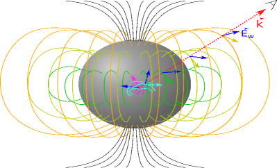
Figure 1: Physical picture of an X-mode EM wave traveling through a neutron star magnetosphere. The magnetic field configuration near the source region, which is near the surface, is complex. As the wave travels outwards, the electric vector adiabatically rotates in such a way that it is always perpendicular to the local magnetic field. At large distances from the neutron star (but still well below the light cylinder), where the plasma density becomes too small to force the electric vector to follow the changing direction of the magnetic field, the polarization position angle is frozen. At this freeze-out radius (not shown in this picture since it is $\gg R_{\rm ns}$), the magnetic field is nearly dipolar and the wave vector is nearly in the radial direction from the center of the star, so the electric vector of the escaping wave is perpendicular to the magnetic dipole moment of the neutron star.

We show that, under suitable conditions, as the wave travels to larger distances from the source, its electric vector adiabatically rotates in such a way that it stays perpendicular to the local magnetic field (and also the wave vector) as shown in Fig. 1. Cheng & Ruderman (1979) considered this “adiabatic walking” phenomenon in the context of radio emission from regular pulsars. In this paper, we show that the same phenomenon is applicable for much stronger magnetic fields (e.g. near a magnetar) and for radio waves with much higher intensity as inferred from FRBs. Beyond a certain distance from the neutron star surface the PA of the wave is frozen; this occurs when the plasma density is too small to be able to force the electric vector to follow the turning and twisting magnetic field lines.

The physics behind adiabatic walking of an EM wave traveling through a neutron star magnetosphere is as follows. The EM wave induces current oscillations, which in turn generate magnetic and electric fields oscillating at the same frequency as the wave. The induced electric field is nearly parallel to the local, non-oscillatory, magnetic field and its magnitude is such that, when appropriate conditions are satisfied as described below, the superposition of the two electric fields remains perpendicular to the local magnetic field.

2.2 Wave Propagation through the Magnetosphere — Linear Regime

In this subsection, we consider the propagation of a weak EM wave in the linear regime where particles in the magnetospheric plasma have non-relativistic speeds. Since in this regime the wave equation can be easily solved analytically and numerically, interesting insight can be gained on the physics of the adiabatic walking. Additional discussion of the linear regime can be found in Appendix A. We extend the discussion to the non-linear regime in the next subsection.

In the following, we decompose vectors into components parallel and perpendicular to the local static magnetic field $\vec{B}$, and identify these components by subscripts $\parallel$ and $\perp$, respectively. The velocity of a particle of charge $q$ and mass $m$ in the presence of a time-varying wave electric field $\vec{E}_{w}\mathrm{exp}(-i\omega t)$ and a static magnetic field $\vec{B}$ is $\vec{v}\mathrm{exp}(-i\omega t)$ (the Fourier components at other frequencies are not relevant), where the components of $\vec{v}$ are given by

$$v_{\parallel}={iqE_{w\parallel}\over m\omega},\ \vec{v}_{\perp}={q\left[-i\omega\vec{E}_{w\perp}+w_{B}\vec{E}_{w}\times\hat{B}\right]\over m(\omega_{B}^{2}-\omega^{2})}.$$ (1)

For a rotating force-free magnetosphere with angular velocity $\vec{\Omega}$, the Goldreich-Julian number density is equal to (Goldreich & Julian, 1969)

$$n_{\rm GJ}=\frac{\vec{\Omega}\cdot\vec{B}}{2\pi qc}.$$ (2)

However, the actual number density of the plasma, $n=n_{+}+n_{-}$, will generally be larger than this by a multiplicity factor $\mathcal{M}$, i.e.

$$n=\mathcal{M}n_{\rm GJ}.$$ (3)

Equivalently, for an electron-position plasma with total number density $n$, the net charge density is equal to $nq/\mathcal{M}$. For the case of a neutron star magnetosphere, where $\omega\ll\omega_{B}$, we can ignore the second-order small terms $\mathcal{O}(\omega^{2}/\omega_{B}^{2})$ in eq. (1). The components of the current density vector $\vec{j}$ can then be obtained from the velocity components in eq. (1):

$$j_{\parallel}={i\omega_{p}^{2}E_{w\parallel}\over 4\pi\omega},\ \vec{j}_{\perp}\approx-{i\omega\omega_{p}^{2}\over 4\pi\omega_{B}^{2}}\left(\vec{E}_{w\perp}+{i\omega_{B}\over\mathcal{M}\omega}\vec{E}_{w}\times\hat{B}\right),$$ (4)

or

$${4\pi i\over\omega}\vec{j}=-{\omega_{p}^{2}\over\omega^{2}}E_{w\parallel}\hat{B}+{\omega_{p}^{2}\over\omega_{B}^{2}}\vec{E}_{w\perp}+{i\omega_{p}^{2}\over\mathcal{M}\omega\omega_{B}}\vec{E}_{w}\times\hat{B}.$$ (5)

This current affects the wave electric field along the propagation path according to the following wave equation (which is obtained by combining Faraday’s and Ampere’s laws)

$${c^{2}\over\omega^{2}}\nabla\times(\nabla\times\vec{E}_{w})-\vec{E}_{w}={4\pi i\over\omega}\vec{j}.$$ (6)

In the following, we first show that the second and third current terms in eq. (5) are negligible. The ratio $\omega_{p}^{2}/\omega_{B}^{2}$ is equal to the reciprocal of the plasma magnetization parameter ($\sigma\equiv B^{2}/4\pi nmc^{2}$). In the neutron star magnetosphere, we find

$$\omega_{p}^{2}/\omega_{\rm B}^{2}\sim 10^{-15}\mathcal{M}B_{0,15}^{-1}P^{-1}(r/100R_{\rm ns})^{3}\lll 1,$$ (7)

where $B_{0}$ is the surface dipole magnetic field (we assume $B\propto r^{-3}$ for $r\gg R_{\rm ns}$). Throughout this paper, we use $B_{0}=10^{15}\,$G as our fiducial value, motivated by the inferred magnetic field strength of nearby magnetars (e.g. Kaspi & Beloborodov, 2017). By equation (7) we see that the second term in the current equation (5) is always negligible. The third term ($\propto\vec{E}_{w}\times\hat{B}$) gives rise to Faraday rotation. Since left and right circularly polarized waves propagate at different phase speeds, the polarization plane rotates by $\Delta\phi=R\omega_{p}^{2}/(\mathcal{M}\omega_{B}c)=4\pi Rnq/\mathcal{M}B$ after a propagation length of $R$. Since $n/\mathcal{M}=n_{\rm GJ}\sim B\Omega/(2\pi qc)$, we find $\Delta\phi\sim 2R\Omega/c=2R/R_{\rm L}$. In §2.3 and §3, we show that the small range of PA variations for FRB 121102 requires the exit point (where the adiabatic walking behavior stops) to be much below the light cylinder radius $R_{\rm L}$. Hence, $\Delta\phi\ll 1\,$rad, and the third term in equation (5) can also be ignored. We include this term in Appendix B for our numerical solutions to the full wave equation and find that its effect on the PA change along the path of the wave is negligible. We are thus left with only the first term in equation (5).

An X-mode EM wave has, by definition, electric field $\vec{E}_{w}$ perpendicular to the $\vec{k}$–$\vec{B}$ plane, hence $E_{w\parallel}=0$. If the wave propagates in a homogeneous plasma, where the magnetic field is uniform, the electric vector remains perpendicular to the $\vec{k}$–$\vec{B}$ plane as the wave propagates, and the first term on the right hand side of equation (5) also vanishes. Thus, the entire right side of equation (5) is essentially zero, and the wave propagates in a straight line with refractive index $\approx 1$, as if in vacuum (all source terms are negligible). In particular, the PA remains constant.

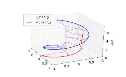
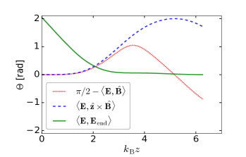
Figure 2: Numerical integration of the 1-D linear wave equation (48) for an example in which the magnetic field rotates around the z-axis at a rate $k_{\rm B}\equiv R_{\rm B}^{-1}$ with pitch angle $\theta=60^{\rm o}$: $\hat{B}=\sin\theta\cos k_{B}z\,\hat{x}+\sin\theta\sin k_{B}z\,\hat{y}+\cos\theta\,\hat{z}$. The boundary conditions are: $\vec{E}_{\rm w}(z=0)=\hat{y}$ (normalized so that $|E_{\rm w}|=1$) and $\mathrm{d}\vec{E}_{\rm w}(z=0)/\mathrm{d}z_{1}=0$. The plasma density is taken to vary with $z$ as: $\omega_{p}^{2}k/\omega^{2}k_{\rm B}=1000(k_{\rm B}z+1)^{-5}$, where $k\equiv\omega/c$. Left Panel: The magnetic field projected in the x–y plane is shown as blue arrows, and the wave electric field is shown as red arrows. Right Panel: The angle between the wave electric vector and the static magnetic field is shown as red dotted line, the angle between the wave electric vector and $\hat{z}\times\hat{B}$ is shown as blue dashed line, and the angle between the wave electric vectors at current location $\vec{E}(z)$ and at the right-hand boundary $\vec{E}_{\rm end}(k_{\rm B}z_{\rm end}=2\pi)$ is shown as green solid line. The angle between two vectors $\vec{A}_{1}$ and $\vec{A}_{2}$ is in general denoted as $\langle\vec{A}_{1},\vec{A}_{2}\rangle\equiv\mathrm{arccos}(\vec{A}_{1}\cdot\vec{A}_{2}/A_{1}A_{2})$. When $\omega_{p}^{2}k/\omega^{2}k_{\rm B}\gg 1$ ($k_{\rm B}z\ll 1$), the wave electric vector adiabatically rotates along with the magnetic field, keeping $\vec{E}_{w}$ nearly aligned with $\vec{k}\times\vec{B}$. As the plasma density drops, when $\omega_{p}^{2}k/\omega^{2}k_{\rm B}\lesssim 2$ ($k_{\rm B}z\gtrsim 2$), the wave electric vector stops rotating and the PA freezes (i.e. the wave propagates as if in vacuum).

The situation is different if we consider an inhomogeneous plasma, in which the direction of the magnetic field changes (by $\sim$1 rad) on a length-scale $R_{\rm B}\gg\lambda$, where $\lambda$ is the wavelength of the EM wave. The plasma density may also change on a similar length-scale. Now, even if a wave starts off with $\vec{E}_{w}$ perpendicular to the $\vec{k}$–$\vec{B}$ plane, it will not remain so, because the magnetic field $\vec{B}$ rotates from its initial direction as the wave propagates. As a result, there will be a non-zero value for the first current term in eq. (5), which is parallel to the local magnetic field. This current induces an electric field which is also parallel to the local magnetic field. The superposition of the induced field and the original wave field causes the electric vector to rotate. As we show, the rotation is such that the wave polarization follows the twisting magnetic field as the wave propagates through the magnetosphere.

For simplicity, we consider a plane wave with electric field amplitude in the form $\vec{E}_{w}(z_{1})\mathrm{e}^{iz_{1}}$, where $z_{1}=kz$ and $k\equiv\omega/c$ is a constant. Then the wave equation (6) becomes

$$\begin{split}2i{\mathrm{d}\over\mathrm{d}z_{1}}(E_{\rm x}\hat{x}+E_{\rm y}\hat{y})&=-{4\pi i\over\omega}(j_{\rm x}\hat{x}+j_{\rm y}\hat{y})\mathrm{e}^{-iz_{1}},\\ E_{\rm z}\hat{z}&=-{4\pi i\over\omega}j_{\rm z}\mathrm{e}^{-iz_{1}},\end{split}$$ (8)

where we have ignored the second-order derivative terms $\mathrm{d}^{2}/\mathrm{d}z_{1}^{2}\sim\mathcal{O}(k^{2}R_{\rm B}^{2})$ (they are included in the numerical calculations in Appendix B). We further simplify the calculation by assuming that the magnetic field is in the x–y plane $\hat{B}(z_{1})=\cos k_{B}z\,\hat{x}+\sin k_{B}z\,\hat{y}$ (where $k_{B}\equiv R_{\rm B}^{-1}$) and hence $E_{\rm z}\equiv 0$ (as we show in Appendix B, the qualitative behavior of adiabatic walking is the same for an arbitrary magnetic field orientation). Then we make use of the current density $4\pi i\omega\vec{j}\approx-\omega_{p}^{2}E_{w\parallel}\hat{B}\mathrm{e}^{iz_{1}}$ (from eq. 5) and the wave equation becomes

$$2i{\mathrm{d}\vec{E}_{\rm w}\over\mathrm{d}z_{1}}\approx{\omega_{\rm p}^{2}\over\omega^{2}}(\vec{E}_{\rm w}\cdot\hat{B})\hat{B}.$$ (9)

Multiplying (dot-product) eq. (9) by $\hat{B}$, we obtain

$${\mathrm{d}\over\mathrm{d}z_{1}}(\vec{E}_{w}\cdot\hat{B})\approx{\omega_{p}^{2}\over 2i\omega^{2}}(\vec{E}_{w}\cdot\hat{B})+\vec{E}_{w}\cdot{\mathrm{d}\hat{B}\over\mathrm{d}z_{1}}.$$ (10)

Since the derivative term on the right hand side can be roughly written as $\vec{E}_{w}\cdot(\mathrm{d}\hat{B}/\mathrm{d}z_{1})\sim E_{w}/kR_{\rm B}$, the equation above can be approximately integrated analytically. Using the X-mode boundary condition $\hat{E}_{w}\cdot\hat{B}|_{z=0}=0$, we obtain

$$\mathrm{Re}\left(\hat{E}_{w}\cdot\hat{B}\right)\sim{2\omega^{2}\over kR_{\rm B}\omega_{p}^{2}}\sin{kz\omega_{p}^{2}\over 2\omega^{2}}.$$ (11)

We see that the angle between the wave electric vector and the magnetic field oscillates with a spatial wavelength of $2\pi\omega c/\omega_{p}^{2}$ and an amplitude $\sim$$\omega^{2}/(kR_{\rm B}\omega_{p}^{2})$. The electric field will follow the direction of the magnetic field so long as the amplitude of the above oscillation is less than about a radian. Therefore, the direction of the electric vector rotates and stays approximately perpendicular to the local magnetic field as long as

$${\omega_{p}^{2}\over\omega^{2}}\gtrsim{{\mathchoice{\smash{\hbox to0.0pt{\raisebox{-1.07639pt}{$\displaystyle\mkern 1.2mu\mathchar 22\relax$}\hss}}\lambda}{\smash{\hbox to0.0pt{\raisebox{-1.07639pt}{$\textstyle\mkern 1.2mu\mathchar 22\relax$}\hss}}\lambda}{\smash{\hbox to0.0pt{\raisebox{-1.07639pt}{$\scriptstyle\mkern 1.2mu\mathchar 22\relax$}\hss}}\lambda}{\smash{\hbox to0.0pt{\raisebox{-1.07639pt}{$\scriptscriptstyle\mkern 1.2mu\mathchar 22\relax$}\hss}}\lambda}}\over R_{\rm B}},\ \ {\mathchoice{\smash{\hbox to0.0pt{\raisebox{-1.07639pt}{$\displaystyle\mkern 1.2mu\mathchar 22\relax$}\hss}}\lambda}{\smash{\hbox to0.0pt{\raisebox{-1.07639pt}{$\textstyle\mkern 1.2mu\mathchar 22\relax$}\hss}}\lambda}{\smash{\hbox to0.0pt{\raisebox{-1.07639pt}{$\scriptstyle\mkern 1.2mu\mathchar 22\relax$}\hss}}\lambda}{\smash{\hbox to0.0pt{\raisebox{-1.07639pt}{$\scriptscriptstyle\mkern 1.2mu\mathchar 22\relax$}\hss}}\lambda}}=\frac{1}{k}={\lambda\over 2\pi}.$$ (12)

A more precise analytical solution of the wave equation under arbitrary boundary conditions is provided in Appendix A, where we show, using an eigenmode analysis, how the wave electric vector rotates as the magnetic field turns. In Appendix B, we present results from numerical integration of the wave equation when $\omega_{p}$ varies with $z$. One example of such a numerical integration is shown in Fig. 2. Here, the magnetic field (only the x–y components are shown as blue arrows) rotates around the z-axis at a rate $k_{\rm B}\equiv R_{\rm B}^{-1}$ with pitch angle $\theta=60^{\rm o}$: $\hat{B}=\sin\theta\cos k_{B}z\,\hat{x}+\sin\theta\sin k_{B}z\,\hat{y}+\cos\theta\,\hat{z}$. The boundary condition is that the wave starts at $z=0$ as a pure X-mode $\vec{E}_{w}(z=0)=\hat{y}$. The plasma density decreases with z as $\omega_{p}^{2}k/\omega^{2}k_{\rm B}=1000(k_{\rm B}z+1)^{-5}$, with $\omega_{p}^{2}$ and $k_{\rm B}$ dropping as $r^{-4}$ and $r^{-1}$ (as a simple example). In a realistic neutron star magnetosphere, the scaling of $\omega_{p}^{2}{k}/\omega^{2}k_{\rm B}$ as a function of radius may be more complicated, but the qualitative result should be the same. For the example shown, we see that the electric vector (red arrows) stays perpendicular to the rotating magnetic field until $\omega_{p}^{2}/\omega^{2}\simeq 2{\mathchoice{\smash{\hbox to0.0pt{\raisebox{-1.07639pt}{$\displaystyle\mkern 1.2mu\mathchar 22\relax$}\hss}}\lambda}{\smash{\hbox to0.0pt{\raisebox{-1.07639pt}{$\textstyle\mkern 1.2mu\mathchar 22\relax$}\hss}}\lambda}{\smash{\hbox to0.0pt{\raisebox{-1.07639pt}{$\scriptstyle\mkern 1.2mu\mathchar 22\relax$}\hss}}\lambda}{\smash{\hbox to0.0pt{\raisebox{-1.07639pt}{$\scriptscriptstyle\mkern 1.2mu\mathchar 22\relax$}\hss}}\lambda}}/R_{\rm B}$ (or $k_{\rm B}z\simeq 2$), beyond which the wave approaches vacuum-like propagation.

In a neutron star magnetosphere, the condition (12) for adiabatic walking of $\vec{E}_{w}$ is violated at some distance from the surface, the freeze-out radius $\widetilde{R}_{\rm fo}$, beyond which the change of PA is negligible. We assume that the magnetic field far from the neutron star surface, but well within the light cylinder ($R_{\rm L}=c/\Omega$), is dominated by the dipole component $B(r)\propto r^{-3}$, as higher order multipoles decline more rapidly. The particle density is a multiple $\mathcal{M}$ of the Goldreich-Julian density $n_{\rm GJ}$, so the freeze-out radius is

$${\widetilde{R}_{\rm fo}\over R_{\rm ns}}\simeq 3.4\times 10^{4}\left[{B_{0,15}\mathcal{M}(R_{\rm B}/\widetilde{R}_{\rm fo})\over\nu_{9}P}\right]^{1/2},$$ (13)

$${\widetilde{R}_{\rm fo}\over R_{\rm L}}\simeq 7\left[{B_{0,15}\mathcal{M}(R_{\rm B}/\widetilde{R}_{\rm fo})\over\nu_{9}P^{3}}\right]^{1/2}.$$ (14)

We see that this estimate of the freeze-out radius in the linear regime may be close to or beyond the light cylinder. At these radii, the magnetic field is dominated by the toroidal rather than the dipolar component of the field, so the PA may vary by a large amount from one burst to another. However, as we show in the next subsection, the adiabatic walking condition for large amplitude FRB waves — in the non-linear regime — is quite different.

2.3 Wave Propagation through the Magnetosphere — Non-linear Regime

A more stringent condition than eq. (12) needs to be satisfied in the case of the high intensity waves present in FRBs. For waves with $qE_{w\parallel}/mc\omega>1$, the particle velocity component parallel to the local magnetic field becomes relativistic. When $E_{w\perp}\gtrsim B$, the transverse velocities also become relativistic (see eq. 1). Relativistic motions break the linear relation between current density and the wave amplitude, so the wave equation becomes highly complicated (numerical simulations of particles’ orbits are needed to calculate the correct current density). In this section, we provide a rough analytical estimate of the condition at which adiabatic walking is terminated for large amplitude EM waves.

Large amplitude EM waves require a large current in order to rotate $\vec{E}_{w}$ and keep it perpendicular to the changing $\vec{k}$–$\vec{B}$ plane. However, the maximum current density (parallel or perpendicular to the magnetic field) that can be supplied by the plasma is $j_{\rm max}\simeq qnc$. If this maximum current oscillates at frequency $\omega$, then the maximum amplitude of the current term on the right-hand side of the wave equation (8) is

$${4\pi\over\omega}j_{\rm max}\simeq{\omega_{\rm p}^{2}\over\omega^{2}}{mc\omega\over q}={\omega_{\rm p}^{2}\over\omega^{2}}{E_{\rm w}\over a_{0}},$$ (15)

where $a_{0}=E_{\rm w}q/mc\omega$ is known as the non-linearity parameter of the EM wave. The wave amplitude at radius $r$ ($\gg$ the source size) from the source is $E_{\rm w}=\sqrt{L/r^{2}c}$, where $L$ is the isotropic equivalent luminosity of an FRB. Hence,

$$a_{0}\equiv{qE_{\rm w}\over mc\omega}\simeq 5.1\times 10^{5}\frac{L_{41}^{1/2}}{r_{7}\nu_{9}}\gg 1,$$ (16)

where we use the typical isotropic equivalent luminosity $L=10^{41}L_{41}\rm\,erg\,s^{-1}$ of bursts detected by Michilli et al. (2018); Gajjar et al. (2018) as a fiducial value.

We take the absolute value of xy components of the wave equation (8) and make use of the maximum current in eq. (15), and obtain

$$2\left|{\mathrm{d}\over\mathrm{d}z_{1}}(E_{\rm x}\hat{x}+E_{\rm y}\hat{y})\right|={4\pi\over\omega}|j_{\rm x}\hat{x}+j_{\rm y}\hat{y}|\lesssim{\omega_{\rm p}^{2}\over\omega^{2}}{E_{\rm w}\over a_{0}}.$$ (17)

To keep $\vec{E}_{w}$ perpendicular to (for X-mode) or inside (for O-mode) the rotating $\vec{k}$–$\vec{B}$ plane, we require $\mathrm{d}(E_{\rm x}\hat{x}+E_{\rm y}\hat{y})/\mathrm{d}z_{1}\sim E_{\rm w}/kR_{\rm B}$. Thus, we obtain the condition for adiabatic walking

$${\omega_{p}^{2}\over\omega^{2}}\gtrsim{a_{0}{\mathchoice{\smash{\hbox to0.0pt{\raisebox{-1.07639pt}{$\displaystyle\mkern 1.2mu\mathchar 22\relax$}\hss}}\lambda}{\smash{\hbox to0.0pt{\raisebox{-1.07639pt}{$\textstyle\mkern 1.2mu\mathchar 22\relax$}\hss}}\lambda}{\smash{\hbox to0.0pt{\raisebox{-1.07639pt}{$\scriptstyle\mkern 1.2mu\mathchar 22\relax$}\hss}}\lambda}{\smash{\hbox to0.0pt{\raisebox{-1.07639pt}{$\scriptscriptstyle\mkern 1.2mu\mathchar 22\relax$}\hss}}\lambda}}\over R_{B}},$$ (18)

which is more stringent than the condition (12) since $a_{0}\gg 1$ (see eq. 16). Thus, the freeze-out radius $R_{\rm fo}$ in the non-linear regime is

$${R_{\rm fo}\over R_{\rm ns}}\simeq 230{B_{0,15}\mathcal{M}(R_{\rm B}/R_{\rm fo})\over PL_{41}^{1/2}},$$ (19)

$${R_{\rm fo}\over R_{\rm L}}\simeq 4.8\times 10^{-2}\,{B_{0,15}\mathcal{M}(R_{\rm B}/R_{\rm fo})\over P^{2}L_{41}^{1/2}}.$$ (20)

We see that $R_{\rm fo}$ here is much smaller than its counterpart in the linear regime $\widetilde{R}_{\rm fo}$ (eq. 13). This is because the extremely high intensity of FRB waves enables them to force their way through the magnetosphere with no change in their PA when the induced electric field by the plasma current is weaker than the parallel component of the wave electric field.

The length scale $R_{\rm B}$ over which the orientation of the magnetic field changes by $\sim$1 rad along the $\vec{k}$ direction depends on the detailed magnetic field configuration in the magnetosphere. In the above estimate, we adopted $R_{\rm B}=R_{\rm fo}$ as our fiducial value but left $R_{\rm B}$ as a free parameter. Near the neutron star surface ($r\sim\mbox{a few}\times R_{\rm ns}$) or near the light cylinder ($r\sim R_{\rm L}$), we may reasonably expect $R_{\rm B}\sim r$. However, this may not hold for $R_{\rm ns}\ll r\ll R_{\rm L}$. For instance, for a magnetosphere with only dipole and quadruple components of equal strength near the surface, the dipole component dominates at increasingly larger radius, and we expect $R_{\rm B}/r\sim r/R_{\rm ns}$ until the toroidal component kicks in near the light cylinder, where we have $R_{\rm B}\sim R_{L}$. Thus, for this particular case, we have $R_{\rm B}\sim\mathrm{min}(r^{2}/R_{\rm ns},R_{\rm L})$. However, without a detailed model of the magnetosphere, the profile $R_{\rm B}(r)$ is currently highly uncertain. Fortunately, as we show in §3, this does not lead to a large uncertainty on the PA of FRBs, as long as $R_{\rm ns}\ll R_{\rm fo}\ll R_{\rm L}$.

We note that the freeze-out radius in eq. (19) is frequency dependent, if the intrinsic emission spectrum $L(\nu)\sim\nu L_{\nu}$ is not flat. Since $R_{\rm fo}\propto L(\nu)^{-1/4}$, the dependence of PA on frequency is rather weak but may still be measurable in the future. For the speculative case $R_{\rm B}\sim\mathrm{min}(r^{2}/R_{\rm ns},R_{\rm L})$ considered above and $\nu L_{\nu}\propto\nu^{\alpha}$, a rough estimate of the PA variation is

$$\nu{\mathrm{d}\mathrm{PA}\over\mathrm{d}\nu}\sim{\alpha\over 4}\mathrm{max}\left({R_{\rm ns}\over R_{\rm fo}},{R_{\rm fo}\over R_{\rm L}}\right),$$ (21)

which gives $\Delta\mathrm{PA}\gtrsim(|\alpha|/4)\sqrt{R_{\rm ns}/R_{\rm L}}\sim 0.3^{\rm o}P^{-1/2}(\Delta\nu/\nu)$, for $|\alpha|\sim\,$order unity. Since the profile $R_{\rm B}(r)$ is highly uncertain, the estimate above is approximate and should be taken with caution. However, the qualitative prediction is that the wavelength dependence of the measured plane of polarization should deviate from the standard $\Theta(\nu)-\Theta(\infty)\propto\nu^{-2}$. A simple way to test this is to measure the PAs with high accuracy at two widely separated frequency bands (e.g. 4 and 8 GHz).

We note that the condition for adiabatic walking in eq. (18) and the freeze-out radius $R_{\rm fo}$ in eq. (19) apply to O-mode as well as X-mode waves. As we show in §3, the small range of PA variation for FRB 121102 requires that the source location to be much below the freeze-out radius $R_{\rm s}\ll R_{\rm fo}$ and the freeze-out radius to be much below the light cylinder $R_{\rm fo}\ll R_{\rm L}$. Near the source location (typically $\omega_{p}\gg\omega$), the induced electric field associated with the plasma current (the first term in eq. 5) cancels with the parallel component of the wave electric field, and hence the wave electric vector $\vec{E}_{w}$ for the O-mode is in the $\vec{k}$–$\vec{B}$ plane and stays perpendicular to $\vec{B}$. The wave magnetic field $\vec{B}_{w}$ is perpendicular to the $\vec{k}$–$\vec{B}$ plane, so we find that the Poynting vector points in the direction of $\vec{E}_{w}\times\vec{B}_{w}\parallel\vec{B}$, i.e. O-mode waves propagate along the local magnetic field near the source region. This can also be seen by calculating the group velocity from the O-mode dispersion relation (e.g. Arons & Barnard, 1986). If the source generates comparable amount of X- and O-mode waves, the high density plasma near the neutron star surface (with $\omega_{p}$, $\omega_{B}\gg\omega$) acts like a polarizing beam splitter which efficiently separates the X-mode (propagating along a straight line) and the O-mode (propagating along the local magnetic field line). If the wave amplitude is small (the limit considered by Arons & Barnard, 1986, in the radio pulsar context), as the plasma density decreases towards large radii, the O-mode phase velocity becomes sub-relativistic (below the typical thermal speed of particles) and hence the wave is severely Landau damped. However, since the extremely intense FRB waves have energy density much larger than what particles (with negligible inertia, see eq. 7) can absorb, the O-mode component may still be able to escape, as long as the magnetic field line extends beyond the freeze-out radius in eq. (19). Still, the energy flux of O-mode waves is severely diluted as the magnetic field lines diverge towards larger radii (the solid angle of the beam increases as $\propto r$ for a pure dipole or faster if higher-order multipoles dominate), so the observer may be biased towards detecting the undiluted, much brighter X-mode flux.

3 FRB Polarization, Progenitor Star Properties, and Radiation Mechanism

Let us consider the FRB source region to be located at a radius $R_{\rm s}$. The physics of wave propagation in the neutron star magnetosphere shown in §2 suggests that the EM waves reaching the observer correspond to the X-mode and will be nearly 100% linearly polarized. As long as the source is located well below the freeze-out radius $R_{\rm s}\ll R_{\rm fo}$, and $\omega_{\rm p},\,\omega_{\rm B}\gg\omega$ near the source, the PA measured by an observer at infinity has no memory of the magnetic field configuration at the source but reflects the direction of the magnetic field at $R_{\rm fo}$; the wave electric vector is parallel to $\hat{k}\times\hat{B}$ at $R_{\rm fo}$. If $R_{\rm s}\ll R_{\rm fo}$ by a factor of 10 or more, then the wave vector at the freeze-out radius is very nearly in the radial direction. In this paper, we assume that the magnetic field at radius $R_{\rm ns}\ll r\ll R_{\rm L}\equiv c/\Omega$ is nearly dipolar, $\vec{B}(\vec{r})\simeq[3\hat{r}(\hat{r}\cdot\vec{m})-\vec{m}]/r^{3}$, where $\vec{m}$ is the magnetic dipole moment of the neutron star. For $R_{\rm ns}\ll R_{\rm fo}\ll R_{\rm L}$, the direction of the wave electric field at $R_{\rm fo}$ is parallel to $\hat{k}\times\hat{B}\parallel\hat{k}\times\hat{m}$, i.e. the PA is perpendicular to the neutron star’s magnetic moment projected in the plane of the sky. For repeating bursts from the same object, the PA would vary from one burst to another, if the magnetic and rotation axes are not parallel.

We denote the angle between the rotational axis and the magnetic dipole moment, or the magnetic inclination, as $\theta_{\rm m}$ and the angle between the rotational axis and the line of sight as $\theta_{\rm k}$ (both at their closest approach). If $\theta_{\rm m}<\theta_{\rm k}$, i.e. the line-of-sight is outside the magnetic inclination cone, the maximum variation of the PA is

$$\pm\Delta\mathrm{PA}_{\rm max}=\pm\,\mathrm{arctan}(\mathrm{tan}\,\theta_{\rm m}/\sin\theta_{\rm k}),$$ (22)

which is close to $\pm\theta_{\rm m}$ if $\theta_{\rm k}$ is of order $\sim$$1\,$rad. On the other hand, if $\theta_{\rm m}>\theta_{\rm k}$, i.e. the line-of-sight is inside the magnetic inclination cone, then the PA can change up to 180^o from burst to burst. The PAs of the repeating FRB 121102 varied by $\pm\Delta\mathrm{PA}_{\rm max}\sim\pm 20^{\rm o}$ for 26 bursts detected over a 7 month period (Michilli et al., 2018; Gajjar et al., 2018). This suggests that (1) the magnetic inclination angle for the neutron star associated with 121102 is $\theta_{\rm m}\lesssim 20^{\rm o}$ and (2) the observer is outside the magnetic inclination cone: $\theta_{\rm m}<\theta_{\rm k}$.

By eq. (19), the condition $R_{\rm fo}\gtrsim 10R_{\rm ns}$ means that $B_{0,15}/P\gtrsim 0.04\,L_{41}^{1/2}\mathcal{M}^{-1}R_{\rm fo}/R_{\rm B}$ or the dipole spin-down time $t_{\rm sd}\lesssim 10^{4}\,\mathrm{yr}\,L_{41}^{-1}(\mathcal{M}R_{\rm B}/R_{\rm fo})^{2}$. We see that this condition can be easily satisfied by young neutron stars, especially if the multiplicity factor $\mathcal{M}\gg 1$ near $R_{\rm fo}$. On the other hand, by eq. (20), the condition $R_{\rm L}\gtrsim 10R_{\rm fo}$ means that

$${B_{0,15}\over P^{2}}\lesssim 2{L_{41}^{1/2}(R_{\rm fo}/R_{\rm B})\over\mathcal{M}}\lesssim 2L_{41}^{1/2},$$ (23)

where we have used $\mathcal{M}\gtrsim 1$ and $R_{\rm B}(R_{\rm fo})\gtrsim R_{\rm fo}$ for the second inequality. Thus, the dipole spin-down luminosity $L_{\rm sd}\lesssim 10^{38}L_{41}\,\mathrm{erg\,s^{-1}}$, and the neutron star is rotating slowly:

$$P\gtrsim(0.7\,\mathrm{sec})\,B_{0,15}^{1/2}L_{41}^{-1/4}.$$ (24)

This constrains the dipole spin-down time to be $t_{\rm sd}\gtrsim(15\mathrm{\,yr})\,B_{0,15}^{-1}L_{41}^{-1/2}$, which is similar to the age constraint from the non-detection of the time derivative of DM due to the expanding supernova remnant (Piro, 2016). We also note that the PA stays nearly constant over the duration of each burst (within error $\delta\mathrm{PA}\lesssim 0.1\,$rad, Michilli et al., 2018). This can be understood if the neutron star is a slow rotator $\Omega\Delta t\lesssim(\delta\mathrm{PA}/\Delta\mathrm{PA}_{\rm max})\pi/2$ or $P>0.01(\Delta t/1\mathrm{\,ms})\,$sec, where $\Delta t$ is the burst duration. This is a weaker constraint than eq. (24).

We conclude that the polarization observations for FRB 121102 suggests: (1) the emitting region is not far from the neutron star’s surface (since $R_{\rm s}\ll R_{\rm fo}\ll R_{\rm L}$); and (2) the neutron star is a slow rotator with period $P\gtrsim(1\mathrm{\,sec})B_{0,15}^{1/2}$ (ignoring the weak dependence of $L_{41}^{-1/4}$). These two pieces of information have interesting implications about the radiation mechanism.

The coherent curvature radiation (or the antenna mechanism) requires high charge density to produce the high FRB luminosities, and strong magnetic field to maintain the coherence of charge bunches, which means it can only operate within a few $R_{\rm ns}$ of the neutron star surface (Kumar et al., 2017; Lu & Kumar, 2018). This model is consistent with the polarization constraints discussed in this paper. In the “cosmic comb” model of Zhang (2017, 2018), the EM waves are produced near the light cylinder of the neutron star and the PA variations among repeating bursts from the same progenitor should be much larger than $\pm 20^{\rm o}$, because the magnetic field direction changes due to stellar rotation and variations of source locations $R_{\rm s}$. Most of the proposed maser mechanisms for FRBs in the literature operate beyond the light cylinder (and hence $R_{\rm s}>R_{\rm fo}$, e.g. Lyubarsky, 2014; Ghisellini, 2017; Waxman, 2017; Beloborodov, 2017), where the magnetic field configuration is far from a regular dipole field and its direction is likely to vary by a large amount from burst to burst. Thus, these models may require fine tuning to explain the observed 100% linear polarization and small variations in PA for the bursts from FRB 121102.

4 Summary

We have proposed a model to explain the recent observations of nearly 100% linear polarization and small variations of the PA for dozens of bursts detected from FRB 121102 over 7 months (in the host-galaxy comoving frame).

In this model, the emission is generated inside the magnetosphere of a strongly magnetized neutron star, with a significant fraction of the power initially in the form of X-mode (with the electric vector perpendicular to the $\vec{k}$–$\vec{B}$ plane). As the radio waves propagate outwards through the neutron star magnetosphere, the electric vector adiabatically rotates and stays perpendicular to the local $\vec{k}$–$\vec{B}$ plane. At sufficiently large distances from the neutron star surface, this “adiabatic walking” behavior stops (and the PA is frozen), when the plasma density is too small to be able to force the electric vector to follow the rotation of the local magnetic field along the propagation. The wave at the exit point is nearly 100% linearly polarized and the PA seen by an observer at infinity is determined by the local magnetic field orientation at this point. The small range of PA variations from FRB 121102 is naturally explained, when the following two conditions are satisfied: (1) the exit point (or freeze-out radius $R_{\rm fo}$) is far away from the neutron star surface and well inside the light cylinder, i.e. $R_{\rm ns}\ll R_{\rm fo}\ll R_{\rm L}$; (2) the emission radius $R_{\rm s}$ is much below the exit point $R_{\rm s}\ll R_{\rm fo}$. Under these two conditions, the magnetic field at the exit point is expected to be nearly dipolar and the wave vector (or the observer’s line-of-sight) is nearly in the radial direction, so the direction of the wave electric field at the exit point is parallel to $\vec{k}\times\vec{B}\parallel\vec{k}\times\vec{m}$, where $\vec{m}$ is the neutron star’s magnetic dipole moment. We see that the PA is always perpendicular to $\vec{m}$ projected in the plane of the sky, independent of the (highly uncertain) magnetic field configuration near the source region.

Since $R_{\rm s}\ll R_{\rm fo}\ll R_{\rm L}$, the emission radius is near the surface of the neutron star. This lends support to the coherent curvature radiation mechanism which requires high charge density $n\gtrsim 10^{17}\rm\,cm^{-3}$ to generate the high luminosity and strong magnetic field $B\gtrsim 10^{14}\,$G to maintain the coherence of charge bunches (Kumar et al., 2017). Many other models in the literature are based on strong collisions of magnetized gas flows near or beyond the light cylinder (Lyubarsky, 2014; Ghisellini, 2017; Waxman, 2017; Zhang, 2018), where the magnetic field orientation is irregular and the PA may vary randomly over a much larger range than observed from FRB 121102.

Under the model proposed in this paper, we use the PA variations from FRB 121102 to constrain the angle between the rotation and magnetic axes (or magnetic inclination) of the underlying neutron star to be $\theta_{\rm m}\lesssim 20^{\rm o}$. Moreover, the requirement $R_{\rm ns}\ll R_{\rm fo}\ll R_{\rm L}$ constrains the rotation period of the neutron star to be $P\gtrsim(1\,\mathrm{sec})\,B_{0,15}^{1/2}$, where $B_{0}=10^{15}B_{0,15}\,$G is the surface dipole magnetic field strength.

We predict that the burst-to-burst variation of PAs from FRB 121102 (at the same frequency) should follow the rotational period of the underlying neutron star (but the burst occurrence is not necessarily periodic). In the future, when more bursts from the repeater are detected with polarization measurements, it should be possible to measure the rotation period, which will provide crucial support for the neutron star nature of FRB progenitors. Other repeating FRBs may have a different range of PA variation, depending on the magnetic inclination $\theta_{\rm m}$ and the observer’s viewing angle with respect to the rotational axis $\theta_{\rm k}$, but the periodic modulation is still controlled by stellar rotation. The detailed PA variation pattern may be used to measure (or constrain) $\theta_{\rm m}$ as well as $\theta_{\rm k}$.

Another prediction of our model is that, for each burst, the PA is weakly frequency-dependent. This is because the freeze-out radius (and hence the local magnetic field orientation) is frequency-dependent, provided the intrinsic spectrum $\nu L_{\nu}$ is not flat. We show that the difference between the PAs measured at $\nu$ and $2\nu$ may be of order $0.1^{\rm o}$ to $1^{\rm o}$, although the exact dependence is highly uncertain (depending on the intrinsic FRB spectrum and the detailed magnetospheric field configuration).

With forthcoming telescopes such as UTMOST (Caleb et al., 2017), Apertif (Maan & van Leeuwen, 2017), FAST (Nan et al., 2011), ASKAP (Bannister et al., 2017), CHIME (The CHIME/FRB Collaboration et al., 2018), the FRB sample size is expected to grow by a factor of 10–100 and many more repeaters may be found and localized. Our predictions could be tested given a sufficiently large sample of bursts with polarization measurements.

Finally, we point out a caveat to our simple model. It is possible that the magnetosphere has significant global twist at radius $r\gg R_{\rm ns}$ (e.g. Thompson et al., 2002). In this case, the magnetic field configuration near the exit point is no longer dipolar (e.g. there may be a significant toroidal component), so the PA variations for repeating bursts from the same object will not follow our predictions, which are based on the dipole field assumption. If this is the case, more sophisticated, time-dependent modeling of the twisted neutron star magnetosphere (e.g. Parfrey et al., 2013; Chen & Beloborodov, 2017) may be needed. Nevertheless, the condition for adiabatic walking (eq. 18) and the location of the freeze-out radius (eq. 19) presented in this paper would still be useful for probing the large scale magnetic field configuration of neutron star magnetospheres.

5 acknowledgments

We thank Emily Petroff and Jason Hessels for useful discussions. WL was supported by the David and Ellen Lee Fellowship at Caltech. RN was supported in part by NSF grant AST-1312651 and by the Black Hole Initiative at Harvard University, which is funded by a grant from the John Templeton Foundation.

Appendix A Analytical solution to the linear wave equation

In this Appendix, we provide an exact solution of the 1-D linear wave equation (eq. 6) along the $z$ direction,

$${c^{2}\over\omega^{2}}{\mathrm{d}^{2}\over\mathrm{d}z^{2}}(E_{x}\hat{x}+E_{y}\hat{y})+\vec{E}_{w}=-{4\pi i\over\omega}\vec{j}.$$ (25)

From eq. (5), the amplitude of the current density is

$${4\pi i\over\omega}\vec{j}\approx-{\omega_{p}^{2}\over\omega^{2}}(\vec{E}_{w}\cdot\hat{B})\hat{B}+{i\omega_{p}^{2}\over\mathcal{M}\omega_{B}\omega}\vec{E}_{w}\times\hat{B},$$ (26)

where we have ignored the high-order small term $\mathcal{O}(\omega_{p}^{2}/\omega_{B}^{2})$, see eq. (7). We consider the simple case of a magnetic field that is purely in the x-y plane and whose direction rotates uniformly as a function of $z$,

$$\begin{split}\vec{B}=B\hat{B}=B(\cos k_{B}z\,\hat{x}+\sin k_{B}z\,\hat{y}),\end{split}$$ (27)

where the magnitude $B$ is independent of $z$. We assume $k_{\rm B}\equiv R_{\rm B}^{-1}\ll\omega/c$ so that the magnetic field rotates slowly compared to the wave phase (we are in the WKB regime). We further assume that the plasma number density $\omega_{p}$ is independent of $z$. A more general case with magnetic field at arbitrary inclination with respect to the z-axis and variable plasma density is considered numerically in Appendix B.

We define two unit vectors parallel and perpendicular to the magnetic field in the x-y plane,

$$\hat{n}_{\parallel}=\hat{B},\ \ \hat{n}_{\perp}=-\sin k_{B}z\,\hat{x}+\cos k_{B}z\,\hat{y},$$ (28)

such that these vectors rotate with the magnetic field, and we decompose the wave electric field amplitude as

$$\vec{E}_{w}=(E_{\parallel}\hat{n}_{\parallel}+E_{\perp}\hat{n}_{\perp}+E_{z}\hat{z})\mathrm{e}^{ikz}.$$ (29)

The z-component of eq. (25) has no derivatives and it gives

$$E_{z}={i\omega_{p}^{2}\over\mathcal{M}\omega\omega_{B}}E_{\perp}.$$ (30)

Inside the neutron star’s magnetosphere, we have $\omega_{p}^{2}/\mathcal{M}\omega\omega_{B}\simeq 4\pi n_{\rm GJ}qc/\omega B\simeq 2/P\nu=2\times 10^{-9}P^{-1}\nu_{9}^{-1}$, where $P$ is the rotational period (in sec) and $\nu_{9}=\nu/\,$GHz is the wave frequency. Thus, the z-component of the wave electric field can be ignored for our problem.

We assume that $E_{\parallel}$ and $E_{\perp}$ are independent of $z$ and look for rotating eigenmodes each with an eigenvalue $k$ that serves the role of a spatial wave-vector. Note that, under this approach, we generally have $k\neq\omega/c$. The imaginary part of $k$ corresponds to exponential damping or growth, and the real part gives the spatial wavelength. The solution to a given physical problem is a superposition of the eigenmodes (each propagating independently) that satisfies the given boundary conditions at $z=0$.

For convenience, below we set $c=1$. The components of the wave equation (25) in the x-y plane are

$$\begin{split}{\mathrm{d}^{2}\over\mathrm{d}z^{2}}\left[(E_{\parallel}\hat{n}_{\parallel}+E_{\perp}\hat{n}_{\perp})\mathrm{e}^{ikz}\right]=\left[(\omega_{p}^{2}-\omega^{2})E_{\parallel}\hat{n}_{\parallel}-\omega^{2}E_{\perp}\hat{n}_{\perp}\right]\mathrm{e}^{ikz}.\end{split}$$ (31)

Apart from the $\mathrm{e}^{ikz}$ factor, the LHS of this equation is $-(k^{2}+k_{B}^{2})(E_{\parallel}\hat{n}_{\parallel}+E_{\perp}\hat{n}_{\perp})+2ikk_{B}(E_{\parallel}\hat{n}_{\perp}-E_{\perp}\hat{n}_{\parallel})$, so we obtain two equations for the parallel and perpendicular components:

$$\begin{split}(k^{2}+k_{B}^{2}+\omega_{p}^{2}-\omega^{2})E_{\parallel}+2ikk_{B}E_{\perp}&=0,\\ (k^{2}+k_{B}^{2}-\omega^{2})E_{\perp}-2ikk_{B}E_{\parallel}&=0.\end{split}$$ (32)

Any non-trivial solution of the wave equation requires the determinant of the above linear equations to be zero, so we obtain the following quadratic equation for $k^{2}$:

$$k^{4}-(2\omega^{2}-\omega_{p}^{2}+2k_{B}^{2})k^{2}-k_{B}^{2}(2\omega^{2}-\omega_{p}^{2})+\omega^{2}(\omega^{2}-\omega_{p}^{2})=0.$$ (33)

The solutions for $k^{2}$ are real when $\Delta=(2\omega^{2}-\omega_{p}^{2}+2k_{B}^{2})^{2}-4[-k_{B}^{2}(2\omega^{2}-\omega_{p}^{2})+\omega^{2}(\omega^{2}-\omega_{p}^{2})]=\omega_{p}^{4}-8k_{B}^{2}\omega_{p}^{2}+16k_{B}^{2}\omega^{2}\geq 0$. The two branches of solutions are

$$k^{2}=\omega^{2}+k_{B}^{2}-{\omega_{p}^{2}\over 2}\pm{\omega_{p}^{2}\over 2}\sqrt{1-{8k_{B}^{2}\over\omega_{p}^{2}}+{16k_{B}^{2}\omega^{2}\over\omega_{p}^{4}}},$$ (34)

which correspond to two eigenmodes of different polarization states propagating towards $+z$ (and there are two more propagating in the opposite direction).

In the following, we discuss two cases: (1) high plasma density $\omega_{p}\gg\omega$ (near the neutron star surface); (2) low plasma density $\omega_{p}\ll\omega$ (far from the neutron star surface).

Case (1): $\omega_{p}\gg\omega\gg k_{\rm B}$; we have $\Delta>0$. The eigenvalues of the two modes are given by

$$k_{+}^{2}\approx\omega^{2}-k_{B}^{2}+{4k_{B}^{2}\omega^{2}\over\omega_{p}^{2}},\ \ k_{-}^{2}\approx\omega^{2}-\omega_{p}^{2}+3k_{B}^{2}-{4k_{B}^{2}\omega^{2}\over\omega_{p}^{2}}.$$ (35)

In this case, the $k_{-}^{2}$($<0$) branch corresponds to the O-mode and doesn’t propagate along the z-direction (because $\omega_{p}\gg\omega$). The $k_{+}$ solution corresponds to the X-mode, and it satisfies

$$\left|{E_{\parallel}\over E_{\perp}}\right|={k_{+}^{2}-\omega^{2}+k_{B}^{2}\over 2k_{+}k_{B}}\approx{2k_{B}\omega\over\omega_{p}^{2}}\ll 1.$$ (36)

This shows that the electric vector of this eigenmode is nearly perpendicular to the local magnetic field. In contrast, the electric vector of the (non-propagating) $k_{-}$ eigenmode is nearly parallel to the field.

Consider a wave with frequency $\omega$ that propagates towards $+z$ and is initialized at $z=0$ with its electric field lying in the $xy$-plane, perpendicular to the local $\vec{B}$. Any electric field in this plane can be written as a linear sum of the two eigenmodes of the problem. In the present case, the sum will be dominated by the $k_{+}$ mode, with only a small amount (of order $\omega k_{B}/\omega_{p}^{2}$) of the $k_{-}$ mode. With increasing $z$, the $k_{-}$ mode will decay (because it is non-propagating), and the wave will become a pure $k_{+}$ mode, with its polarization rotating so as to remain nearly perpendicular to the magnetic field. Thus the wave adiabatically walks with the rotating field.

Case (2): $\omega\gg\omega_{p}\gg k_{\rm B}$; $\Delta>0$ for this case as well. The square-root term in solutions (34) has different asymptotic behaviors in the following two sub-regimes. The first regime is when $\omega_{p}^{4}/16k_{B}^{2}\omega^{2}\gg 1$, and we have

$$k^{2}\approx\omega^{2}+k_{B}^{2}-{\omega_{p}^{2}\over 2}\pm\left({\omega_{p}^{2}\over 2}-2k_{B}^{2}+{4k_{B}^{2}\omega^{2}\over\omega_{p}^{2}}\right),$$ (37)

that is,

$$\begin{split}k_{+}^{2}&\approx\omega^{2}-k_{B}^{2}+{4k_{B}^{2}\omega^{2}\over\omega_{p}^{2}}\\ &\Longrightarrow\ \left|{E_{\parallel}\over E_{\perp}}\right|=\left|{k_{+}^{2}-\omega^{2}+k_{B}^{2}\over 2k_{+}k_{B}}\right|\approx{2k_{B}\omega\over\omega_{p}^{2}}\ll 1,\\ k_{-}^{2}&\approx\omega^{2}-\omega_{p}^{2}+3k_{B}^{2}-{4k_{B}^{2}\omega^{2}\over\omega_{p}^{2}}\\ &\Longrightarrow\left|{E_{\perp}\over E_{\parallel}}\right|=\left|{k_{-}^{2}-\omega^{2}+\omega_{p}^{2}+k_{B}^{2}\over 2k_{-}k_{B}}\right|\approx{2k_{B}\omega\over\omega_{p}^{2}}\ll 1.\end{split}$$ (38)

We can see that in this regime, the $k_{+}$ and $k_{-}$ solutions correspond to the X-mode ($E_{\perp}$ dominates) and O-mode ($E_{\parallel}$ dominates) respectively. Both of these are propagating modes, and their electric vectors rotate adiabatically to keep $\vec{E}$ nearly perpendicular to $\vec{B}$ and $\vec{k}$ (X-mode) or in the $\vec{k}$–$\vec{B}$ plane (O-mode). As in the previous case, a wave that starts off with its electric field perpendicular to $\vec{B}$ at $z=0$ will adiabatically rotate with the field and will remain nearly perpendicular to $\vec{B}$ as it propagates.

The second regime is when $\omega_{p}^{4}/16k_{B}^{2}\omega^{2}\ll 1$. Here we find

$$k^{2}\approx\omega^{2}+k_{B}^{2}-{\omega_{p}^{2}\over 2}\pm 2k_{B}\omega\left(1+{\omega_{p}^{4}\over 32k_{B}^{2}\omega^{2}}-{\omega_{p}^{2}\over 4\omega^{2}}\right).$$ (39)

If we retain only the lowest order terms, we have $k_{\pm}^{2}\approx\omega^{2}\pm 2k_{B}\omega-\omega_{p}^{2}/2$ and $k_{\pm}\approx\omega\pm k_{B}-\omega_{p}^{2}/4\omega$, which means

$$\begin{split}\left({E_{\parallel}\over E_{\perp}}\right)_{\pm}&={k_{\pm}^{2}-\omega^{2}+k_{B}^{2}\over 2ikk_{B}}\approx{-\omega_{p}^{2}\pm 4k_{B}\omega\over 4ikk_{B}}\\ &\approx i\left(\mp 1+{\omega_{p}^{2}\over 4k_{B}\omega}\right).\end{split}$$ (40)

The two eigenmodes have electric fields

$$\begin{split}\vec{E}_{\pm}&=(E_{\parallel\pm}\hat{n}_{\parallel}+E_{\perp\pm}\hat{n}_{\perp})\mathrm{e}^{ik_{\pm}z}\\ &\approx\left[{i\omega_{p}^{2}\over 4k_{B}\omega}\hat{n}_{\parallel}\mp i\hat{n}_{\parallel}+\hat{n}_{\perp}\right]E_{\perp\pm}\mathrm{e}^{i(\omega\pm k_{B}-\omega_{p}^{2}/4\omega)z}\\ &=\left[{i\omega_{p}^{2}\over 4k_{B}\omega}\hat{n}_{\parallel}\mathrm{e}^{\pm ik_{B}z}+(\hat{y}\mp i\hat{x})\right]E_{\perp\pm}\mathrm{e}^{i\omega z(1-\omega_{p}^{2}/4\omega^{2})},\end{split}$$ (41)

where $E_{\perp\pm}\approx(1\pm\omega_{p}^{2}/8k_{B}\omega)/\sqrt{2}$ are determined by normalization $|\vec{E}_{\pm}|=1$. Since $\omega_{p}^{2}/4k_{B}\omega\ll 1$, the first term corresponds to a weak rotation of the electric vector at the rate of $k_{B}$. The second term represents the commonly used left and right circularly polarized modes. If we ignore the first term, any linearly polarized wave at $z=0$ can be decomposed into the superposition of $\vec{E}_{+}$ and $\vec{E}_{-}$ with equal amplitudes. Then, as the wave propagates, it stays linearly polarized with the PA unchanged. However, because of the first term, the PA rotates by $\sim\omega_{p}^{2}\Delta z/(2\omega)$ when the wave travels a distance $\Delta z\lesssim k_{B}^{-1}$.

To summarize, we have shown that, in the linear regime, the wave electric vector adiabatically walks with the twisting magnetic field as long as the following condition is satisfied: $\omega_{p}^{2}\gtrsim k_{B}\omega/2$. When the plasma density drops such that $\omega_{p}^{2}\ll k_{B}\omega/2$, the electric vector stops corotating with the plasma magnetic field and asymptotically approaches vacuum-like propagation. The transition from adiabatic walking to polarization freeze-out happens when $\omega_{p}^{2}\sim ck_{B}\omega$ (where we have restored the $c$). Writing $k_{B}=2\pi/R_{B}$ and using $\omega\simeq ck=c/{\mathchoice{\smash{\hbox to0.0pt{\raisebox{-1.07639pt}{$\displaystyle\mkern 1.2mu\mathchar 22\relax$}\hss}}\lambda}{\smash{\hbox to0.0pt{\raisebox{-1.07639pt}{$\textstyle\mkern 1.2mu\mathchar 22\relax$}\hss}}\lambda}{\smash{\hbox to0.0pt{\raisebox{-1.07639pt}{$\scriptstyle\mkern 1.2mu\mathchar 22\relax$}\hss}}\lambda}{\smash{\hbox to0.0pt{\raisebox{-1.07639pt}{$\scriptscriptstyle\mkern 1.2mu\mathchar 22\relax$}\hss}}\lambda}}$, the freeze-out occurs when

$$\frac{\omega_{p}^{2}}{\omega^{2}}\gtrsim\frac{{\mathchoice{\smash{\hbox to0.0pt{\raisebox{-1.07639pt}{$\displaystyle\mkern 1.2mu\mathchar 22\relax$}\hss}}\lambda}{\smash{\hbox to0.0pt{\raisebox{-1.07639pt}{$\textstyle\mkern 1.2mu\mathchar 22\relax$}\hss}}\lambda}{\smash{\hbox to0.0pt{\raisebox{-1.07639pt}{$\scriptstyle\mkern 1.2mu\mathchar 22\relax$}\hss}}\lambda}{\smash{\hbox to0.0pt{\raisebox{-1.07639pt}{$\scriptscriptstyle\mkern 1.2mu\mathchar 22\relax$}\hss}}\lambda}}}{R_{B}},$$ (42)

which agrees with equation (12).

To derive the condition (18) in the main text, we start with equation (26) and consider the parallel component of the current:

$$j_{\parallel}=\frac{i\omega_{p}^{2}}{4\pi\omega}E_{\parallel}.$$ (43)

The X-mode is dominated by the perpendicular field, so $E_{\perp}\approx E_{w}$, the total electric field. Equations (36) and (38) show that, for both Case (1) and Case (2) with adiabatic walking, the ratio of $E_{\parallel}$ to $E_{\perp}$ is small and equal to $2ck_{B}\omega/\omega_{p}^{2}$ (again restoring $c$). Thus, the parallel current can be written as

$$|j_{\parallel}|\approx\frac{ck_{B}}{2\pi}E_{w}.$$ (44)

As argued in the main text, the maximum current that the plasma can support is $qnc$. Therefore, polarization freeze-out will occur once we have

$$\frac{ck_{B}}{2\pi}E_{w}\gtrsim qnc,$$ (45)

which can be rewritten as the condition

$$\frac{\omega_{p}^{2}}{\omega^{2}}\gtrsim\frac{a_{0}{\mathchoice{\smash{\hbox to0.0pt{\raisebox{-1.07639pt}{$\displaystyle\mkern 1.2mu\mathchar 22\relax$}\hss}}\lambda}{\smash{\hbox to0.0pt{\raisebox{-1.07639pt}{$\textstyle\mkern 1.2mu\mathchar 22\relax$}\hss}}\lambda}{\smash{\hbox to0.0pt{\raisebox{-1.07639pt}{$\scriptstyle\mkern 1.2mu\mathchar 22\relax$}\hss}}\lambda}{\smash{\hbox to0.0pt{\raisebox{-1.07639pt}{$\scriptscriptstyle\mkern 1.2mu\mathchar 22\relax$}\hss}}\lambda}}}{R_{B}},\ \ a_{0}\equiv\frac{qE_{w}}{mc\omega}.$$ (46)

This agrees with equation (18).

Appendix B Numerical solution to the linear wave equation

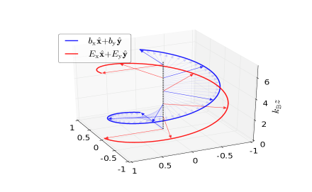
Figure 3: Numerical solution to the wave equation (48) with constant $\omega_{\rm p}^{2}k/\omega^{2}k_{\rm B}=1000$, $\theta=60^{\rm o}$ and boundary conditions: $\vec{E}_{\rm w}(z=0)=\hat{y}$ (normalized so that $|E_{\rm w}|=1$) and $\mathrm{d}\vec{E}_{\rm w}/\mathrm{d}z_{1}(z=0)=0$. Left Panel: The wave electric vector (red arrows) rotates with the turning of static magnetic field (blue arrows, only the projection in the x-y plane is show) in a way such that $\vec{E}_{w}$ stays parallel to $\hat{z}\times\vec{B}$. Right Panel: The angle between the wave electric vector and $\hat{z}\times\hat{B}$ is very small (blue, which agrees will the analytical estimation in eq. 11), and the angle between the wave electric vector and the static magnetic field is very close to $\pi/2$ (red). Both angles oscillate rapidly on length scale of $(\omega^{2}/\omega_{\rm p}^{2})k^{-1}=10^{-3}k_{\rm B}^{-1}$.

In this Appendix, we numerically integrate the linear wave equation in one dimension along the z-axis, for variable plasma density and magnetic field at arbitrary inclination with respect to the z-axis.

We combine the current in eq. (5) and the general wave equation (6), and obtain

$${c^{2}\over\omega^{2}}{\mathrm{d}^{2}\over\mathrm{d}z^{2}}(E_{x}\hat{x}+E_{y}\hat{y})+\vec{E}_{w}={\omega_{p}^{2}\over\omega^{2}}(\vec{E}_{w}\cdot\hat{B})\hat{B}-{i\omega_{p}^{2}\over\mathcal{M}\omega_{B}\omega}\vec{E}_{w}\times\hat{B},$$ (47)

where we have ignored the high order small current term $\mathcal{O}(\omega_{p}^{2}/\omega_{B}^{2})$ (see eq. 7). In the following, we take a different approach from Appendix A and write the wave amplitude in Cartesian basis as $[E_{x}(z_{1})\hat{x}+E_{y}(z_{1})\hat{y}+E_{z}(z_{1})\hat{z}]\mathrm{exp(iz_{1})}$, where $z_{1}\equiv kz$ and $k\equiv\omega/c$ is a constant. Then we obtain a set of coupled ordinary differential equations

$$\left({\mathrm{d}^{2}\over\mathrm{d}z_{1}^{2}}+2i{\mathrm{d}\over\mathrm{d}z_{1}}\right)\left[{\begin{array}[]{c}E_{\rm x}\\ E_{\rm y}\\ \end{array}}\right]={\overset{\leftrightarrow}{A}\over\omega^{2}/\omega_{\rm p}^{2}-b_{\rm z}^{2}}\cdot\left[{\begin{array}[]{c}E_{\rm x}\\ E_{\rm y}\\ \end{array}}\right],$$ (48)

where

$$\overset{\leftrightarrow}{A}=\left[{\begin{array}[]{cc}b_{\rm x}b_{\rm x}&b_{\rm x}b_{\rm y}+\chi\\ b_{\rm x}b_{\rm y}-\chi&b_{\rm y}b_{\rm y}\\ \end{array}}\right],\,\chi={i\omega\over\mathcal{M}\omega_{\rm B}}({\omega_{\rm p}^{2}\over\omega^{2}}-1)b_{\rm z},$$ (49)

$$E_{\rm z}={(E_{\rm x}b_{\rm x}+E_{\rm y}b_{\rm y})b_{\rm z}-{i\omega\over\mathcal{M}\omega_{\rm B}}(E_{\rm x}b_{\rm y}-E_{\rm y}b_{\rm x})\over\omega^{2}/\omega_{\rm p}^{2}-b_{\rm z}^{2}},$$ (50)

and $b_{\rm x}$, $b_{\rm y}$, $b_{\rm z}$ are the Cartesian components of the unit vector $\hat{B}$ (along the direction of the static magnetic field).

We consider the orientation of the magnetic field rotating as a function of $z$ at arbitrary pitch angle $\theta$ with respect to the z-axis

$$\hat{B}=\sin\theta\cos k_{\rm B}z\,\hat{x}+\sin\theta\sin k_{\rm B}z\,\hat{y}+\cos\theta\,\hat{z},$$ (51)

where $k_{\rm B}\equiv R_{\rm B}^{-1}\ll k$ (in the WKB regime). If the plasma properties ($\theta$, $k_{\rm B}$, $\omega_{p}^{2}/\omega$, $\omega/\mathcal{M}\omega_{B}$) are known at every point $z>0$, we can integrate the wave equation (48) from the left-hand boundary $z=0$.

We use $\theta=60^{\rm o}$ and $k_{\rm B}/k=10^{-4}$ for the two cases presented in this paper. The (X-mode) boundary conditions are: $\vec{E}_{\rm w}(z=0)=\hat{y}$ (normalized so that $|E_{\rm w}(z=0)|=1$), $\mathrm{d}\vec{E}_{\rm w}/\mathrm{d}z_{1}(z=0)=0$. We are interested in the situation where $\omega\ll\omega_{\rm B}$ and $\mathcal{M}\geq 1$, so the terms of order $\omega/\mathcal{M}\omega_{\rm B}$ are very small. In all cases presented in this paper, we have tested different choices of $\omega/\mathcal{M}\omega_{\rm B}=10^{-3}$ (corresponding to $B\gtrsim 10^{6}\,$G), $10^{-6}$ and $10^{-9}$, and our results are practically the same.

In the realistic neutron star magnetosphere, the ratio $k_{\rm B}/k$ is much smaller than $10^{-4}$ near the freeze-out radius, and our calculations (limited by computational cost) can be appropriately scaled to arbitrarily small $k_{\rm B}/k$. In Fig. 3, we show the case with constant $\omega_{p}^{2}{k}/\omega^{2}k_{\rm B}=1000$, which corresponds to the propagation below the freeze-out radius given by eq. (13) in the linear regime. In Fig. 2, we show the case with decreasing ratio $\omega_{p}^{2}{k}/\omega^{2}k_{\rm B}=1000(k_{\rm B}z+1)^{-5}$ along the propagation. For this case, we can see that the transition from adiabatic walking (rotating electric vector) to vacuum-like propagation (non-rotating electric vector) occurs at $k_{\rm B}z\simeq 2$ and is quite sharp.

References

- Arons & Barnard (1986) Arons, J., & Barnard, J. J. 1986, ApJ, 302, 120
- Bhandari et al. (2018) Bhandari, S., Keane, E. F., Barr, E. D., et al. 2018, MNRAS, 475, 1427
- Bannister et al. (2017) Bannister, K. W., Shannon, R. M., Macquart, J.-P., et al. 2017, ApJL, 841, L12
- Beloborodov & Thompson (2007) Beloborodov, A. M., & Thompson, C. 2007, ApJ, 657, 967
- Beloborodov (2017) Beloborodov, A. M. 2017, ApJL, 843, L26
- Caleb et al. (2017) Caleb, M., Flynn, C., Bailes, M., et al. 2017, MNRAS, 468, 3746
- Caleb et al. (2018) Caleb, M., Keane, E. F., van Straten, W., et al. 2018, arXiv:1804.09178
- Champion et al. (2016) Champion, D.-J., Petroff, E., Kramer, M., et al. 2016, MNRAS
- Chatterjee et al. (2017) Chatterjee, S., Law, C. J., Wharton, R. S., et al. 2017, arXiv:1701.01098
- Chen & Beloborodov (2017) Chen, A. Y., & Beloborodov, A. M. 2017, ApJ, 844, 133
- Cheng & Ruderman (1979) Cheng, A. F., & Ruderman, M. A. 1979, ApJ, 229, 348
- Farah et al. (2018) Farah, W., Flynn, C., Bailes, M., et al. 2018, arXiv:1803.05697
- Gajjar et al. (2018) Gajjar, V., Siemion, A. P. V., Price, D. C., et al. 2018, arXiv:1804.04101
- Ghisellini (2017) Ghisellini, G. 2017, MNRAS, 465, L30
- Goldreich & Julian (1969) Goldreich, P., & Julian, W. H. 1969, ApJ, 157, 869
- Kaspi & Beloborodov (2017) Kaspi, V. M., & Beloborodov, A. M. 2017, ARA&A, 55, 261
- Katz (2014) Katz, J. I. 2014, Phys. Rev. D, 89, 103009
- Katz (2016) Katz, J. I. 2016, Modern Physics Letters A, 31, 1630013
- Katz (2018) Katz, J. I. 2018, arXiv:1804.09092
- Keane & Petroff (2015) Keane, E. F., & Petroff, E. 2015, MNRAS, 447, 2852
- Kulkarni et al. (2014) Kulkarni, S. R., Ofek, E. O., Neill, J. D., Zheng, Z., & Juric, M. 2014, ApJ, 797, 70
- Kumar et al. (2017) Kumar, P., Lu, W., & Bhattacharya, M. 2017, MNRAS, 468, 2726
- Law et al. (2017) Law, C. J., Abruzzo, M. W., Bassa, C. G., et al. 2017, ApJ, 850, 76
- Lazar, Nakar, & Piran (2009) Lazar A., Nakar E., Piran T., 2009, ApJ, 695, L10
- Lorimer et al. (2007) Lorimer, D. R., Bailes, M., McLaughlin, M. A., Narkevic, D. J., & Crawford, F. 2007, Science, 318, 777
- Lu & Kumar (2018) Lu, W., & Kumar, P. 2018, MNRAS, 477, 2470
- Luan & Goldreich (2014) Luan, J., & Goldreich, P. 2014, ApJL, 785, L26
- Lyubarsky (2014) Lyubarsky, Y. 2014, MNRAS, 442, L9
- Maan & van Leeuwen (2017) Maan, Y., & van Leeuwen, J. 2017, arXiv:1709.06104
- Marcote et al. (2017) Marcote, B., Paragi, Z., Hessels, J. W. T., et al. 2017, ApJL, 834, L8
- Masui et al. (2015) Masui, K., Lin, H.-H., Sievers, J., et al. 2015, Nature, 528, 523
- Michilli et al. (2018) Michilli, D., Seymour, A., Hessels, J. W. T., et al. 2018, Nature, 553, 182
- Nan et al. (2011) Nan, R., Li, D., Jin, C., et al. 2011, International Journal of Modern Physics D, 20, 989
- Narayan & Kumar (2009) Narayan R., Kumar P., 2009, MNRAS, 394, L117
- Narayan & Piran (2012) Narayan R., Piran T., 2012, MNRAS, 420, 604
- Oostrum et al. (2017) Oostrum, L. C., van Leeuwen, J., Attema, J., et al. 2017, The Astronomer’s Telegram, 10693,
- Parfrey et al. (2013) Parfrey, K., Beloborodov, A. M., & Hui, L. 2013, ApJ, 774, 92
- Petroff et al. (2015) Petroff, E., Bailes, M., Barr, E. D., et al. 2015, MNRAS, 447, 246
- Petroff et al. (2016) Petroff, E., Barr, E. D., Jameson, A., et al. 2016, PASA, 33, e045
- Petroff et al. (2017) Petroff, E., Burke-Spolaor, S., Keane, E. F., et al. 2017, MNRAS, 469, 4465
- Piro (2016) Piro, A. L. 2016, ApJL, 824, L32
- Rane et al. (2016) Rane, A., Lorimer, D. R., Bates, S. D., et al. 2016, MNRAS, 455, 2207
- Ravi et al. (2016) Ravi, V., Shannon, R. M., Bailes, M., et al. 2016, Science, 354, 1249
- Scholz et al. (2016) Scholz, P., Spitler, L. G., Hessels, J. W. T., et al. 2016, ApJ, 833, 177
- Spitler et al. (2016) Spitler, L. G., Scholz, P., Hessels, J. W. T., et al. 2016, Nature, 531, 202
- Tendulkar et al. (2017) Tendulkar, S. P., Bassa, C. G., Cordes, J. M., et al. 2017, ApJL, 834, L7
- The CHIME/FRB Collaboration et al. (2018) The CHIME/FRB Collaboration, :, Amiri, M., et al. 2018, arXiv:1803.11235
- Thompson et al. (2002) Thompson, C., Lyutikov, M., & Kulkarni, S. R. 2002, ApJ, 574, 332
- Thornton et al. (2013) Thornton, D., Stappers, B., Bailes, M., et al. 2013, Science, 341, 53
- Waxman (2017) Waxman, E. 2017, ApJ, 842, 34
- Zhang (2017) Zhang, B. 2017, ApJL, 836, L32
- Zhang (2018) Zhang, B. 2018, ApJL, 854, L21