SCExAO/CHARIS Near-Infrared Direct Imaging, Spectroscopy, and Forward-Modeling of $\kappa$ And b: A Likely Young, Low-Gravity Superjovian Companion

Abstract

We present SCExAO/CHARIS high-contrast imaging/$JHK$ integral field spectroscopy of $\kappa$ And b, a directly-imaged low-mass companion orbiting a nearby B9V star. We detect $\kappa$ And b at a high signal-to-noise and extract high precision spectrophotometry using a new forward-modeling algorithm for (A-)LOCI complementary to KLIP-FM developed by Pueyo et al. (2016). $\kappa$ And b’s spectrum best resembles that of a low-gravity L0–L1 dwarf (L0–L1$\gamma$). Its spectrum and luminosity are very well matched by 2MASSJ0141-4633 and several other 12.5–15 $M_{\rm J}$ free floating members of the 40 $Myr$-old Tuc-Hor Association, consistent with a system age derived from recent interferometric results for the primary, a companion mass at/near the deuterium-burning limit (13${}^{+12}_{-2}$ M_J), and a companion-to-primary mass ratio characteristic of other directly-imaged planets ($q$ $\sim$ 0.005${}^{+0.005}_{-0.001}$). We did not unambiguously identify additional, more closely-orbiting companions brighter and more massive than $\kappa$ And b down to $\rho$ $\sim$ 0$\farcs$3 (15 au). SCExAO/CHARIS and complementary Keck/NIRC2 astrometric points reveal clockwise orbital motion. Modeling points towards a likely eccentric orbit: a subset of acceptable orbits include those that are aligned with the star’s rotation axis. However, $\kappa$ And b’s semimajor axis is plausibly larger than 75 au and in a region where disk instability could form massive companions.

Deeper $\kappa$ And high-contrast imaging and low-resolution spectroscopy from extreme AO systems like SCExAO/CHARIS and higher resolution spectroscopy from Keck/OSIRIS or, later, IRIS on the Thirty Meter Telescope could help clarify $\kappa$ And b’s chemistry and whether its spectrum provides an insight into its formation environment.

1 Introduction

The past decade of facility high-contrast imaging systems and now dedicated extreme adaptive optics-based planet imagers have revealed the first direct detections of planets around nearby, young stars (Marois et al., 2008, 2010a; Lagrange et al., 2010; Kuzuhara et al., 2013; Carson et al., 2013; Quanz et al., 2013; Rameau et al., 2013; Currie et al., 2014a, 2015a; Macintosh et al., 2015; Chauvin et al., 2017; Keppler et al., 2018). Their range of masses (2–15 $M_{\rm J}$) and orbital separations (10–150 au) make them key probes of jovian planet formation models (e.g. Boss, 1997; Kenyon and Bromley, 2009). The companions’ photometry reveal clear differences with field brown dwarfs and evidence for extremely cloudy and/or dusty atmospheres (Currie et al., 2011).

Integral field spectrographs (IFS) further clarify the atmospheric properties of young planet-mass companions, revealing tell-tale signs of low surface gravity from sharper, more point-like $H$-band peaks (e.g. Barman et al., 2011; Allers and Liu, 2013). Hotter, early L type planets at very young ages (1–10 $Myr$) may also exhibit a red, rising slope through $K$-band, also a sign of low surface gravity (Canty et al., 2013; Currie et al., 2014a). While the near-infrared (near-IR) spectra of some cooler L/T and T-type directly-imaged planets show evidence for more extreme clouds, more vigorous chemical mixing, and/or lower gravities than found in (nearly all of) even the youngest, lowest mass objects formed by cloud fragmentation (e.g. Currie et al., 2011; Bonnefoy et al., 2016; Rajan et al., 2017; Chauvin et al., 2018), L-type young directly-imaged planets can be nearly indistinguishable from free floating, planet-mass analogues with identical ages (e.g. Allers and Liu, 2013; Chilcote et al., 2017; Dupuy et al., 2018).

The directly-imaged low-mass companion to the B9V star $\kappa$ Andromedae ($\kappa$ And b; Carson et al., 2013) is an object whose properties could be clarified by new, high-quality IFS data. Based on $\kappa$ And b’s luminosity and the primary’s proposed status as a sibling of HR 8799 in the 30–40 $Myr$-old Columba association (Zuckerman et al., 2011; Bell et al., 2015), Carson et al. estimated its mass to be 12.8 $M_{\rm J}$. Using broadband photometry, Bonnefoy et al. (2014a) suggest a spectral type of M9–L3 and find some evidence for photospheric dust but fail to constrain $\kappa$ And b’s surface gravity and admit a wider range of possible ages and thus masses. The Project 1640 IFS-based follow-up study by Hinkley et al. (2013) question whether $\kappa$ And is a Columba member, derive a much older age of 220 $Myr$, and argue that $\kappa$ And b’s spectrum suggests the companion is not planetary mass. However, subsequent studies based on the primary admit the possibility that the system is young ($t$ $\sim$ 30–40 $Myr$; and thus the companion could be low mass) (David and Hillenbrand, 2015; Brandt and Huang, 2015). Furthermore, CHARA interferometry precisely constraining the rotation rate, gravity, temperature, and luminosity and comparing these properties to stellar evolution models favor a young age (Jones et al., 2016). New, higher quality IFS data for $\kappa$ And b can better clarify whether the companion shares properties (e.g. surface gravity) more similar to the young planet-mass objects or older, deuterium burning brown dwarfs.

In this study, we report new $JHK$ direct imaging and spectroscopy of $\kappa$ And b obtained with the Subaru Coronagraphic Extreme Adaptive Optics project coupled to the CHARIS integral field spectrograph (Jovanovic et al., 2015a; Groff et al, 2013). We analyze these data and combine them with archival Keck/NIRC2 imaging to yield new constraints on $\kappa$ And b’s atmosphere and orbit.

2 SCExAO/CHARIS Data for $\kappa$ And

2.1 Observations and Basic Data Reduction

SCExAO targeted $\kappa$ And on UT 8 September 2017 with the CHARIS integral field spectrograph operating in low-resolution ($R$ $\sim$ 20), broadband (1.13–2.39 $\mu m$) mode (Peters et al., 2012; Groff et al, 2013). SCExAO/CHARIS data were acquired in pupil tracking/angular differential imaging (ADI) mode (Marois et al., 2006) with the star’s light blocked by the Lyot coronagraph with the 217 mas diameter occulting spot. Satellite spots, diffractive attenuated copies of the stellar PSF, were generated by applying a 25 nm amplitude modulation on the deformable mirror. (Jovanovic et al., 2015b). Exposures consisted of 42 co-added 20.6 $s$ frames covering a modest total parallactic angle rotation of $\sim$ 10.5${\arcdeg}$. The data were taken under good, “slow” seeing conditions: 0$\farcs$4–0$\farcs$5 in $V$ band with 2–4 ms^-1 winds. The real-time AO telemetry monitor recorded the residual wavefront error after SCExAO’s correction, implying typical exposure-averaged $H$-band Strehl Ratios of 90-92%.

We used the CHARIS Data Reduction Pipeline (CHARIS DRP; Brandt et al., 2017) to convert raw CHARIS data into data cubes consisting 22 image slices spanning wavelengths from 1.1 $\mu m$ to 2.4 $\mu m$. Calibration data provided a wavelength solution; using the the robust ‘least squares’ method described in Brandt et al., we extracted CHARIS data cubes. Contemporaneous Keck/NIRC2 observations of HD 1160 calibrated CHARIS astrometry, yielding a spaxel scale of 0$\farcs$0162, a $\rho$ $\sim$ 1.05″ radius field of view, and north position angle offset of -2.2^o (see Appendix A).

Basic image processing steps – e.g. image registration, sky subtraction – were carried out using our CHARIS IDL-based data reduction pipeline, which will later be released alongside a future release of the Python-based CHARIS DRP (i.e. the “CHARIS Post-Processing Pipeline”) and were described in recent SCExAO/CHARIS science/instrumentation studies (Currie et al., 2018; Goebel et al., 2018). Inspection of the data cubes revealed little residual atmospheric dispersion and exposure-to-exposure motion of the centroid position; the spot modulation amplitude translated into a channel-dependent spot extinction of $atten_{\lambda}$ = 2.72$\times$10^-3 $\times$($\lambda$/1.55 $\mu m$)^-2.

To spectrophotometrically calibrate each data cube, we considered both stellar atmosphere models and the widely-used Pickles et al. (1998) library adopted in our previous CHARIS papers (Currie et al., 2018; Goebel et al., 2018), in the GPI Data Reduction Pipeline (Perrin et al., 2014), and in P1640 analysis of $\kappa$ And b’s near-IR spectrum in Hinkley et al. (2013). As described in the Appendix B, for B9V and some other spectral types the Pickles et al. library lacks direct measurements in the near-IR and instead adopts an extrapolation from shorter wavelengths that would translate into a miscalibrated companion spectrum. As an alternative, we used a Kurucz stellar model atmosphere (Castelli and Kurucz, 2004). Parameters were tuned to closely match those determined from interferometry (Jones et al., 2016): $T_{\rm eff}$ = 11000 $K$, log(g) = 4.0.

As shown in Figure 1, $\kappa$ And b is visible in raw CHARIS data, with a peak emission roughly three times (0.5–5 times) that of the local speckle intensity in wavelength-collapsed images (individual channels). In $H$ band, the companion is about as well separated from the speckle halo as it was in earlier, Fall 2016 SCExAO/HiCIAO data obtained with the vortex coronagraph shown in Figure 6a of Kuhn et al. (2018). Inspection of our raw broadband images shows that $\kappa$ And b would be marginally visible without processing at smaller separations down to $\rho$ $\sim$ 0$\farcs$5.

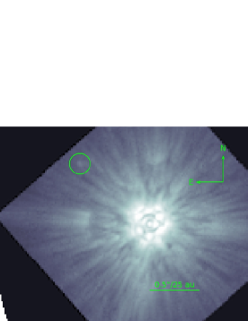
Figure 1: A characteristic broadband (wavelength-collapsed) CHARIS image shown in a log color stretch (minimum value to maximum value). The companion $\kappa$ And b is visible without any PSF subtraction techniques or even unsharp masking applied. The stellar halo is well suppressed at an intensity roughly or just slightly higher than that of $\kappa$ And b down to $\rho$ $\approx$ 0$\farcs$5.

2.2 Point-Spread Function (PSF) Subtraction and Spectral Extraction

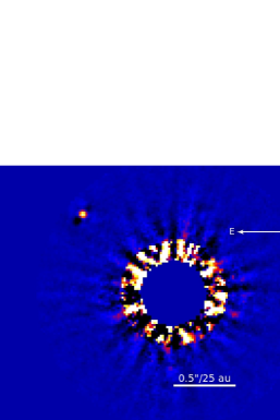
Figure 2: Detection of $\kappa$ And b from SCExAO/CHARIS utilizing only ADI (not SDI) (left) with very conservative settings in A-LOCI for PSF subtraction and (right) with a more aggressive reduction using A-LOCI. $\kappa$ And b is detected with a SNR of 88 and 110. We extract the spectrum of $\kappa$ And b from the conservative reduction. The residuals are significantly higher at $\rho$ $\sim$ 0$\farcs$3–0$\farcs$5 for the conservative reduction largely due to a combination of local masking, aggressive covariance matrix truncation, and the large rotation gap. Throughput is lower and self-subtraction footprints along the azimuthal direction are stronger for the aggressive reduction due to its lack of masking, its less aggressive covariance matrix truncation, and smaller rotation gap.

To further suppress the stellar halo and yield a high signal-to-noise (SNR) detection of $\kappa$ And b in each channel, we employed advanced point-spread function (PSF) subtraction techniques. We performed PSF subtraction using Adaptive, Locally-Optimized Combination of Images (A-LOCI Currie et al., 2012) – a derivative of the LOCI algorithm (Lafrenière et al., 2007). In this approach, the PSF $I$ of image slice $i$ in an annular region $s$ is subtracted from a weighted linear combination of other image slice regions $\{j\}$ in the sequence:

$${\cal R}_{i,s}=I_{i,s}-\sum_{j}\alpha_{ij,s}I_{j,s}~{}.$$ (1)

In LOCI, the coefficients $\alpha_{ij,s}$ are determined solving from a system of linear equations that minimize the residuals between the target slice and references in an “optimization” region $o$, the solution to the linear system

$$\mathbf{A}\cdot\boldsymbol{\alpha}=\mathbf{b}~{},$$ (2)

where the covariance matrix A and column matrix b are

$${\rm A}_{jl}=\sum_{{\rm pixels}~{}k}I_{jk,o}I_{lk,o}\quad{\rm and}\quad{\rm b}_{j}=\sum_{{\rm pixels}~{}k}I_{ik,o}I_{jk,o}~{},$$ (3)

by a simple matrix inversion. The subtraction zone $s$ is typically a subset of pixels comprising optimization region $o$. The set of image slices $J$ used to construct a weighted reference PSF is typically defined by those fulfilling a rotational gap criterion, where a point-source in region $s$ has moved some fraction of a PSF footprint, $\delta$$\times$$\theta_{FWHM}$, between frames $i$ and $j$ due to parallactic angle motion.

In A-LOCI, this approach is modified in several ways. First, it optionally removes pixels within the subtraction zone $s$ from the optimization zone $o$, which increase point source throughput and, as shown in Appendix C makes algorithm forward-modeling more tractable (“local masking”/“a moving pixel mask”; Marois et al., 2010b; Currie et al., 2012). Second, it redefines the covariance matrix A and column matrix b, selecting the $n$ image slices best-correlated with the target image slice over each region $o$. Third, it rewrites A using singular value decomposition (SVD) as U$\Sigma$V, truncating the diagonal matrix , $\Sigma$, at singular values greater than some fraction of the maximum singular value ($svd_{lim}$) before inverting and thus allowing a low(er)-rank approximation of the covariance matrix A:

$$\boldsymbol{\alpha}=(\mathbf{U}\mathbf{\Sigma_{>\mathit{svd_{lim}}}}\mathbf{V})^{-1}\cdot\mathbf{b}.$$ (4)

We performed two reductions: 1) a conservative one focused on obtaining a high-fidelity spectrum and 2) an aggressive one that maximizes the achieved contrast in our data. In our first “conservative” approach, we processed data in annular regions for each wavelength channel independently (ADI-only). The annular subtraction zone of depth $dr$ = 10 was masked, a weighted reference PSF was constructed from a 75 PSF footprint “optimization” area exterior to the subtraction zone, and the diagonal terms of the covariance matrix were truncated at $svd_{lim}$ = 2$\times$10^-6$\times$max($\Sigma$). In our second “aggressive” approach, we performed an A-LOCI reduction first utilizing ADI only and then performing spectral differential imaging (SDI) on the ADI residuals. For the ADI component, we shrunk the rotation gap, optimization area, and SVD cutoff, leaving the $dr$ = 5 pixel-deep subtraction zone unmasked. For the SDI component, we scaled each image slice in the ADI-reduced data cube by wavelength and subtracted the residuals with A-LOCI. Instead of an angular gap, we imposed a radial gap of $\delta$ = 0.65, masked the subtraction zone, and constructed a weighted reference PSF from pixels at the same separation as the subtraction zone but different angles as in Currie et al. (2017a) from the pseudo-inverse of A truncated at $svd_{lim}$ = 1$\times$10^-6$\times$max($\Sigma$). In all cases, given the limited number of exposures, we did not truncate the reference set by cross-correlation. Finally, we de-scaled, rotated and combined the ADI/SDI-subtracted image slices together for a final data cube and final broadband (wavelength-collapsed) image.

To assess and correct for signal loss of $\kappa$ And b due to processing and thus extract a calibrated spectrum and precise astrometry, we forward-modeled planet spectra through the observing sequence (e.g. Pueyo, 2016). Our formalism extends that of Brandt et al. (2013), is detailed in Appendix C, and considers both self-subtraction due to displaced copies of the planet signal weighted by coefficients $\alpha_{ij}$ and perturbations of these coefficients $\beta_{ij}$ due to the planet signal.

2.3 High Signal-to-Noise Detection of $\kappa$ And b with SCExAO/CHARIS and Extracted Spectrum

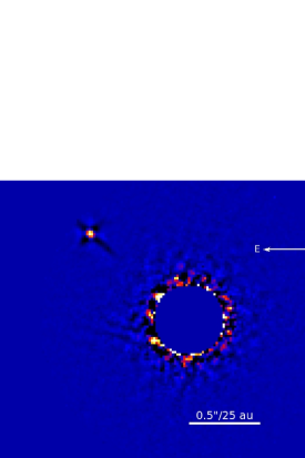
Figure 3: Detection of $\kappa$ And b utilizing both ADI and SDI (SNR $\sim$ 210). Although the planet now exhibits strong radial self-subtraction footprints due to SDI, its signal loss due to SDI is nearly negligible due to CHARIS’ wide spectral bandpass.

Figures 2 and 3 display wavelength-collapsed CHARIS images reduced using “conservative” and “aggressive” PSF subtraction approaches and utilizing ADI only and in conjunction with SDI. The companion $\kappa$ And b is easily visible at a high SNR (88-210) in the wavelength-collapsed images at a projected separation of $\rho$ $\approx$ 0$\farcs$91 and decisively detected in all channels in all reductions. Except for channel 6 in the most conservative reduction ($\lambda_{\rm o}$ = 1.376 $\mu$m; SNR $\sim$ 6.4), the detection significance exceeds 10$\sigma$ in all channels for all reductions.

To extract the spectrum for $\kappa$ And b from the conservative (ADI-only) reduction, we defined the signal from aperture photometry with $r_{\rm ap}$ = 0.5 $\lambda$/D around the best-estimated position (as determined from the wavelength-collapsed image). We repeated these steps with slight modifications to our algorithm settings to confirm repeatability of the spectrum to a level less than the intrinsic SNR of the detection in each channel. We confirmed that a negative copy of the extracted planet spectrum, when inserted into our sequence prior to processing, fully nulled $\kappa$ And b in all channels after PSF subtraction.

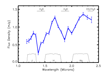
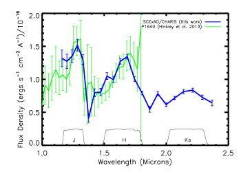
Figure 4: (left) SCExAO/CHARIS spectrum of $\kappa$ And b extracted from our conservative (ADI-only) reduction shown in $F_{\rm\nu}$ units with regions attributed major molecular absorption in substellar objects overplotted. (right) SCExAO/CHARIS $\kappa$ And b spectrum compared to that from P1640 presented in Hinkley et al. (2013) and plotted in $F_{\rm\lambda}$ units. Both panels show transmission profiles for major near-IR passbands $JHK_{\rm s}$ (MKO). The CHARIS error bars do not include an additional $\sim$ 5% absolute calibration uncertainty.

Figure 4 displays the extracted CHARIS spectrum in units of mJy (left) and (right) compares our spectrum to that from P1640 as extracted in Hinkley et al. (2013) in units of ergs s^-1 cm² Å^-1. The spectrum is fully listed in Appendix D. The CHARIS spectrum shows regions of suppressed flux in between the $JHK$ passbands and a slight suppression beyond 2.3 $\mu m$, attributed to water and water/CO absorption in early L dwarfs (e.g. Cushing et al., 2005; Cruz et al., 2018). The $H$ band spectrum is characterized by a clear peak at $\lambda$ $\sim$ 1.65 $\mu$m and steep drop at redder wavelengths; the $K$ band spectrum exhibits a plateau or slightly rising flux between 2.1 and 2.2 $\mu$m.

The CHARIS spectrum shows slight differences with that extracted from P1640 over wavelengths where the two overlap (1.1–1.8 $\mu$m). The CHARIS spectrum is more peaked in $H$ band than in the P1640 data at $\sim$ 1.65 $\mu$m, with significantly lower flux density at 1.7–1.8 $\mu$m. Section 7.1 discusses the sources of these differences.

Following Greco and Brandt (2016), we assess the nature of residual noise affecting our extracted spectrum by estimating the spectral covariance at $\kappa$ And b’s location in our final data cube. We divided each channel by the residual noise profile and then computed the cross-correlation between pairs of channels $i$ and $j$ in 2 $\lambda$/D-wide annulus at $\kappa$ And b’s location, masking pixels within 2 $\lambda$/D of the companion:

$$\psi_{i,j}=\frac{<\bar{C_{i}{C_{j}}}>}{\sqrt{<\bar{C_{i}^{2}}><\bar{C_{j}^{2}}>}}.$$ (5)

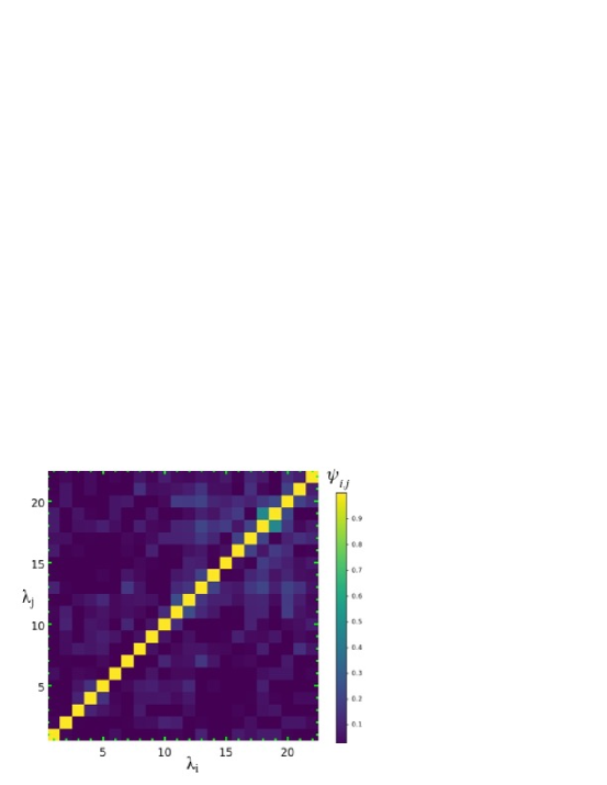
Figure 5: The correlation matrix $\psi_{\rm i,j}$ as a function of spectral channel. Off-diagonal elements identify the effect of residual correlated noise. With the exception of a few channels (e.g., a slight coupling of channel 17 and 18), the residuals are nearly spatially uncorrelated.

Figure 5 displays the spectral covariance at the location of $\kappa$ And b. Except for a few red channels (e.g. 16 and 17 in K-band), the covariance sharply drops for off-diagonal elements. The functional form for the covariance proposed by Greco and Brandt 2016 consists of spatially ($\rho$) and spectrally ($\lambda$) correlated noise with characteristic lengths ($\sigma_{\rho}$ and $\sigma_{\lambda}$) and an uncorrelated term A_δ:

$$\psi_{i,j}=A_{\rho}e^{-0.5((\lambda_{i}-\lambda_{j})/\sigma_{\rho})^{2}}+A_{\lambda}e^{-0.5((\lambda_{i}-\lambda_{j})/\sigma_{\lambda})^{2}}+A_{\delta}.$$ (6)

The data are best fit by A_ρ = 0.12, A_λ = 0.05, A_δ= 0.82, $\sigma_{\rho}$ = 0.65, and $\sigma_{\lambda}$ = 0.24: thus, the residual speckle noise is well-suppressed and poorly coupled between different wavelengths. At smaller separations where the rotation gap criterion results in far poorer speckle suppression, the noise is dominated by the correlated components (e.g. at $\rho$ $\sim$ 0$\farcs$45, A_ρ + A_λ = 0.56 and A_δ= 0.44).

To estimate broadband photometry for $\kappa$ And b, we convolve the spectrum with the Mauna Kea Observatories $JHK$ filter functions binned down to the resolution of CHARIS. The companion’s apparent magnitude in major MKO passbands is $J$= 15.84 $\pm$ 0.09, $H$ = 15.01 $\pm$ 0.07, and $K_{\rm s}$ = 14.37 $\pm$ 0.07. Its $J$-$H$ and $J$-$K_{\rm s}$ colors agree with previous estimates from Carson et al. (2013), Hinkley et al. (2013), and Bonnefoy et al. (2014a). In the 2MASS photometric system, its colors are slightly redder (e.g. $J_{\rm 2MASS}$ - $K_{\rm s,2MASS}$ = 1.52).

3 New and Archival Keck/NIRC2 $K_{\rm s}$ Band Astrometric Data

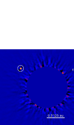
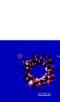
Figure 6: (left) Detection of $\kappa$ And b from from archival 2013 Keck/NIRC2 data (PI J. A. Johnson) and (right) from December 2017 Keck/NIRC2 data. The image scale is equivalent to that in previous figures; $\kappa$ And b is at a wider angular separation in the archival data than in the SCExAO/CHARIS data.

To supplement $\kappa$ And b’s astrometry derived from SCExAO/CHARIS data, we measure its position in well-calibrated data obtained recently and in prior epochs using Keck coupled with the NIRC2 camera. First, we obtained new Keck/NIRC2 coronagraphic imaging of $\kappa$ And on UT 8 December 2017 in the K_s filter using the 0$\farcs$6 diameter coronagraphic spot. Data consisted of coadded 30-second exposures covering 13.6^o of parallactic angle motion. Basic image processing follows previous methods utilized for $\kappa$ And observations taken with Keck/NIRC2 drawn from Currie et al. (2011), including dark subtraction, flat-fielding, distortion corrections, and image registration (Bonnefoy et al., 2014a). We used A-LOCI with local masking of the subtraction zone to produce a nearly unattenuated detection of $\kappa$ And b (SNR = 27).

Second, we searched for and identified $\kappa$ And $K_{\rm s}$ band data from the Keck Observatory Archive taken on UT 18 August 2013 (PI John Asher Johnson), consisting of 15 20-second exposures. A visual inspection of these data reveals $\kappa$ And b, and they fill in the gap in astrometric measurements between the CHARIS data set (September 2017) and those from Bonnefoy et al. (2014a). We use A-LOCI with local masking and a rotation gap of 1 PSF footprint to subtract the stellar halo, yielding a high throughput detection and high-precision astrometry. The SNR is comparable to or slightly higher than that from the discovery paper (Carson et al., 2013) and other early detections (e.g. Burress et al., 2013). Third, we report unpublished astrometry for $\kappa$ And b from data taken on UT 3 November 2012 published in Bonnefoy et al. (2014a).

The 2017 and 2013 epoch detections are shown in Figure 6. Astrometry in each data set assumed a 9.971 mas pixel scale and north position angle offset of 0.262^o for the 2017 data and 9.952 mas pixel scale and north position angle offset of 0.252^o for earlier data sets (Service et al., 2016; Yelda et al., 2010). Comparing the position of $\kappa$ And b in these two data sets and with CHARIS clearly shows that the companion’s projected separation is decreasing with time.

4 Empirical Constraints on $\kappa$ And b’s Atmospheric Properties

To analyze $\kappa$ And b’s spectrum, we adopt a three-pronged approach, 1) comparing it to optically-anchored L dwarf spectral templates covering a range of gravities, 2) comparing it to a large library of empirical JHK spectra for MLT dwarfs, and 3) assessing gravity from spectral indices. The templates provide a baseline qualitative assessment for $\kappa$ And b’s spectral type and gravity. The libraries further clarify these parameters, identifying a set of best-fit objects, some of which have well-estimated ages and masses. The spectral indices serve as a quantitative estimate of gravity.

For empirical comparisons, we quantify the goodness-of-fit by comparing $\kappa$ And b’s spectrum $f$ to the $k$th weighted comparison spectrum $F_{k}$, choosing the multiplicative factor $\alpha_{k}$ that minimizes $\chi^{2}$ and considering errors in both $\kappa$ And b and the comparison spectrum:

$$\chi^{2}_{k}=(f-\alpha F_{k})^{T}C_{k}^{-1}(f-\alpha F_{k})$$ (7)

Here, $C_{k}$ is the covariance matrix, where diagonal terms correspond to measured errors in both $\kappa$ And b ($\sigma_{f}$) and those estimated for the comparison spectrum ($\sigma_{F_{k}}$) and off-diagonal terms consider the coupling of $\kappa$ And b spectral errors between different channels as parameterized in §2.3.

Table 1: Fits to Cruz et al. (2018) Spectral Standards

Spectral Type	Gravity Class	Hcont,CHARIS	H2K, CHARIS	$\chi_{\nu}^{2}$ (total)	$\chi_{\nu}^{2}$ ($H$+$K$)
L0	field	0.935	1.050	3.76	3.72
L0	$\beta$	0.945	1.032	1.68	2.41
L0	$\gamma$	0.971	1.020	1.26	1.40
L1	field	0.912	1.056	2.90	3.55
L1	$\beta$	0.926	1.056	1.80	1.71
L1	$\gamma$	0.949	1.037	2.84	1.41
L2	field	0.896	1.076	2.03	2.44
L2	$\gamma$	0.960	1.009	5.10	3.32
L3	field	0.890	1.075	1.51	1.78
L3	$\gamma$	0.947	1.031	3.50	1.91
L4	field	0.867	1.075	2.28	1.86
L4	$\gamma$	0.940	1.037	15.32	10.96
L6	field	0.847	1.110	3.36	2.94
L7	field	0.855	1.109	5.92	3.19
L8	field	0.794	1.172	5.00	6.63

Note. — The $\chi_{\nu}^{2}$ values are calculated assuming 15 degrees of freedom for fitting of the JHK peaks and 10 for just $H$ and $K$. Entries in bold identify those that fit the data to within the 95% confidence limit.

We define acceptly-fitting models as those with a $\chi^{2}$ per degree of freedom less than the 95% confidence limit: $\chi^{2}_{\nu}$ $\leq$ $\chi^{2}_{\nu,95\%C.L.}$ To avoid regions heavily contaminated by tellurics and/or covering wavelengths with missing data, we primarily focused on a set of 16 CHARIS spectral channels covering the MKO JHK bandpasses. In a second pass, we focus on 11 spectral channels covering $H$ and $K$ only, where broadband spectral features may be diagonistic of gravity (Allers and Liu, 2013; Canty et al., 2013). In Chilcote et al. (2017), this is referred to as the “restricted fit”. Finally, as a check on our results, for empirical comparisons we perform an “unrestricted” fit the full JHK spectrum, allowing the scaling to freely vary between the three passbands, to account for the intrinsic variation the J–K spectral energy distribution at a given spectral type (e.g. Knapp et al., 2004).

4.1 Comparisons to Template L dwarf Spectra

Cruz et al. (2018) compute L dwarf near-infrared spectral average templates, constructed (for each spectral type) from a set from of characteristic optically spectral-typed substellar objects. The templates cover L0-L4 and L6-L8 field objects, L0-L1 intermediate-gravity dwarfs (L0-L1$\beta$), and low-gravity L0-L4 dwarfs (L0-L4$\gamma$). The sample of near-infrared spectra comprising each template show typical variations on the order of $\sim$ 5% across $J$-$K$; inspection of empirical spectra comprising some templates showed variations in spectral shape at similar levels. Thus, we set a floor to the spectrophotometric uncertainty of 5%.

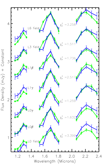
Figure 7: Comparisons between $\kappa$ And b (blue) and spectral templates (green) from Cruz et al. (2018). The wavelengths plotted are the sixteen used to define $\chi^{2}$. The L0$\gamma$ template provides the best fit; L0$\gamma$ and L1$\gamma$ best reproduce the shape of the $H$ and $K$-band portions of the spectra.

Table 1 and Figure 7 compares how well $\kappa$ And b matches each Cruz et al. template. Overall, the L0$\gamma$ template best fits $\kappa$ And b’s spectrum ($\chi^{2}_{\nu}$ = 1.22), while the L3 field dwarf template marginally fits and the L0–L1$\beta$ templates are marginally inconsistent at the 95% confidence limit. When focused more on gravity-sensitive $H$ and $K$ band, low gravity templates L0$\gamma$ and L1$\gamma$ fit the best; the L1$\beta$ and L3 field templates are marginally consistent while the L3$\gamma$ and L4 field templates are marginally excluded. The agreement with the overall shape of $\kappa$ And b’s spectrum drives the small $\chi^{2}$ values for the L0$\gamma$ and L3 field templates; the shape of both the $H$ and $K$-band spectra are clearly better fit by the L0$\gamma$ template.

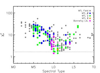
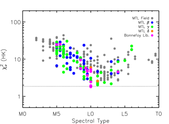
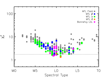
Figure 8: (top) For the JHK passbands and just HK (middle), the $\chi^{2}_{\nu}$ statistic comparing $\kappa$ And b to substellar object spectra, including field (gray), intermediate (blue), low (green), and very-low (orange) gravity objects listed in the Montreal Spectral Library and predominantly young, low-mass objects from the VLT/SINFONI library described in Bonnefoy et al. (2014a). Horizontal lines identify the $\chi^{2}_{\nu}$ limits below which objects match $\kappa$ And b’s spectrum at the 95% confidence limit. (bottom) The $\chi^{2}_{\nu}$ distribution when allowing the J, H, and K-band portions of the empirical spectrum to be separately scaled.

4.2 Comparisons to Empirical MLT Dwarf Spectra

Our sample of empirical spectra primarily draws from the Montreal Spectral Library and the Bonnefoy et al. (2014b) VLT spectral library . The Montreal library covers MLT dwarfs with field, intermediate ($\beta$), low ($\gamma$), and very low ($\delta$) gravities characteristic of old ($\sim$ Gyr), intermediate aged ($\sim$ 100 Myr), young ($\sim$ 10–100 Myr), and very young ($<$ 10 Myr) low-mass stars and substellar objects, respectively. The Montreal data draw from multiple sources presenting spectra reduced using multiple instruments, including Gagne et al. (2014, 2015), Robert et al. (2016), Artigau et al. (2010), Delorme et al. (2012), and Naud et al. (2014). The Bonnefoy library focuses on objects near the M/L transition (M6-L1) having intermediate to (very-)low gravities ($\beta$$\gamma$$\delta$) with spectra drawn from a single source (VLT/SINFONI) reduced in a uniform manner. We trimmed our Montreal library sample of objects with very low SNR or those with substantial telluric contamination at the edges of the JHK passbands, leaving 360 objects. Since the Bonnefoy et al. (2014b) library nominally lists a spectrum normalized in $J$ or $HK$, we focused only on those objects whose spectra can be relatively calibrated across $JHK$ (12 objects).

Figure 8 displays $\chi^{2}_{\nu}$ as a function of spectral type for the $JHK$ and $HK$ restricted fits (top and middle panels) and the $JHK$ unrestricted fit (bottom panel), quantitatively showing how well each empirical spectrum matches $\kappa$ And b’s spectrum. The distribution for the restricted fits shows a clear minimum for L0-L1 spectral types with low surface gravity with 1 (2) objects formally satisfying the 95% confidence limit for the full $JHK$ ($HK$) spectrum. In both plots, another 2-3 objects lie just above this limit, all of which are likewise L0-L1 objects with low gravity. For the unrestricted fit, more objects cluster at or below the 95% confidence limit, including the $\sim$ 10 $Myr$-old objects UScoCTIO108 B (M9.5 $\gamma$, Bonnefoy library; Bejar et al., 2008) and 2MASS J12074836-3900043 (L1$\delta$, Montreal library; Gagne et al., 2014). The $\chi^{2}_{\nu}$ minimum for the unrestricted fit is broader (M9 to L2–L4), although L0–L1$\gamma$ objects still dominate the subset of those that fit well.

Table 2 lists the best-fitting spectra and their properties from the restricted fits. 2MASSJ0141-4633 (Kirkpatrick et al., 2006) – a L0–L1$\gamma$ dwarf and member of the Tucana-Horologium Association– provides the best fit. In general, the sample of best-fitting objects listed in Table 2 is dominated by confirmed and candidate L0–L1$\gamma$ Tuc-Hor members.

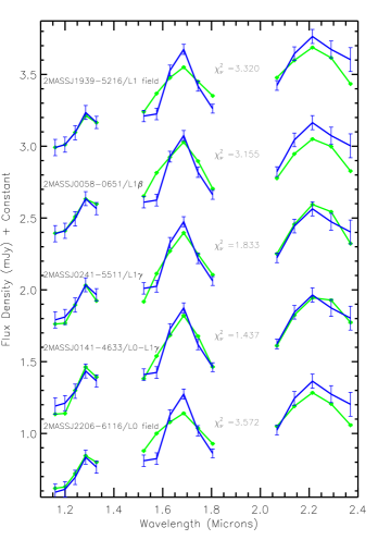
Figure 9: Comparisons between $\kappa$ And b (blue) and a representative sample of L0-L1 dwarfs with different gravity classes (green) from the Montreal and Bonnefoy spectral libraries. The L0–L1$\gamma$ object 2MASSJ0141-4633 provides the best overall match to $\kappa$ And b.

Table 2: Properties of the Best-Fitting Substellar Objects

Name	$\chi^{2}_{\nu}$	$\chi^{2}_{\nu}$	SpT	Hcont.	H2K	Assoc.	Age	log(L/L⊙)	$T_{\rm eff}$ (K)	log(g)	Mass (MJ)
	(Total)	(H+K)		Index	Index		(Myr)	(Approx.)		(Approx.)
2MASSJ0141-4633	1.43	1.81	L0-L1$\gamma$	0.962	1.027	Tuc-Hor	40${}^{+5}_{-19}$	-3.58	1899 $\pm$ 123	4.1–4.2	13–15
									1800${}^{+200}_{-100}$
2MASSJ0120-5200	2.25	2.24	L1$\gamma$	1.032	1.049	Tuc-Hor	40${}^{+5}_{-19}$	-3.65	1685 $\pm$ 145	4.1–4.2	12.5–14
2MASSJ0241-5511	1.83	2.59	L1$\gamma$	1.015	1.034	Tuc-Hor	40${}^{+5}_{-19}$	-3.67	1731 $\pm$ 151	4.1–4.2	12.5–14
2MASSJ0440-5126	1.79	2.64	L0$\gamma$	1.003	1.006	Tuc-Hor? (53)	40${}^{+5}_{-19}$?	-3.63?	1600–2000	4.1–4.2?	13–15?
2MASSJ2033-5635	1.71	2.44	L0$\gamma$	0.945	1.034	Tuc-Hor??a	??	??	1600–2000	??	??
2MASSJ2325-0259	1.45	2.03	L1$\gamma$	1.040	1.067	AB Dor? (65)	130–200?	-3.80?b	1700–1900	4.7–4.9?	30–40?b
2MASSJ2322-6151B	1.94	2.26	L1$\gamma$	1.015	1.083	Tuc-Hor	40${}^{+5}_{-19}$	-3.68	1793 $\pm$ 50	4.1–4.2	12.5-14

Note. — Spectra for all objects match $\kappa$ And b’s at 99.7% confidence for the $JHK$ restricted fit, the $HK$ restricted fit, and the $JHK$ unrestricted fit. Secure moving group members are defined from Banyan-$\Sigma$ as those with $>$ 95% probability in a given group. Those with $>$ 50% are noted with ”?”: the Banyan-$\Sigma$ probability is listed in parentheses. Temperatures are listed from Faherty et al. (2016) (first entry) or Bonnefoy et al. (2014a) (second entry) where available; otherwise, they are estimated from the range in temperatures from Gonzales et al. (2018). If given, luminosities, surface gravities, and masses are calculated assuming the nominal object distance, the K-band bolometric correction from Todorov et al. (2010), and the Baraffe et al. (2003) luminosity evolution models. a) Previously identified as a Tuc-Hor member, Banyan-$\Sigma$ favors a field object ($\sim$ 75% vs. 25%). No parallax is given. Thus its membership and properties depending on distance are noted with a ”??”. b) Mass and luminosity estimated using the “optimal” kinematic distance for moving group membership.

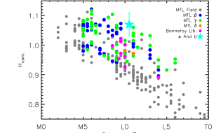
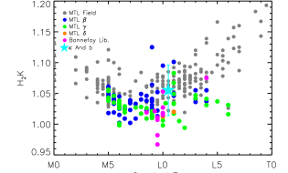
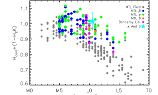
Figure 10: Revised (for CHARIS) $H$-continuum (top), $H_{2}K$ (middle) gravity-sensitive spectral indices, and a combined index (bottom) for $\kappa$ And b (cyan star) and the comparison sample. Large values for the $H$-continuum index at a given spectral type suggest low gravity; small values for the $H_{2}K$ index generally low gravity, albeit less decisively. Uncertainties are shown for $\kappa$ And b; those for the comparison sample are not shown for clarity but are typically on the order of the symbol size.

To illustrate how $\kappa$ And b’s spectrum best resembles that of a low-gravity L0-L1 dwarf, Figure 9 compares it to 2MASSJ0141-4633 (the best-fitting object with small spectrophotometric errors) and a representative set of L0-L1 objects with small errors and different gravity classes. The shape of the $\kappa$ And b $H$ and $K$ spectra strongly favor that of a low-gravity object, as the $H$-band spectrum is far sharper than any field object and the red half of the $K$-band spectrum flatter. All other field and intermediate-gravity L0-L1 dwarfs more poorly match $\kappa$ And b. Other L0-L1$\gamma$ dwarfs have $\chi^{2}$ values that are still characteristically smaller than L0-L1 field objects (see Figure 8).

4.3 Quantitative Assessments of Surface Gravity Using Spectral Indices

We use multiple near-infrared spectral indices to assess the companion’s surface gravity: the $H$-continuum index ($H$-cont) defined by Slesnick et al. (2004) and the $H_{\rm 2}$$K$ index described by Canty et al. (2013). The $H$-cont index is defined from two measurements of the “continuum” flux ($\lambda_{1}$ = 1.470 $\mu m$, $\lambda_{2}$ = 1.670 $\mu m$) and a measurement of the “line” flux at 1.560 $\mu m$:

$$H_{\rm cont}=\biggl{[}\frac{\lambda_{\rm line}-\lambda_{\rm 1}}{\lambda_{\rm 2}-\lambda_{\rm 1}}F_{\lambda_{2}}+\frac{\lambda_{\rm 2}-\lambda_{\rm line}}{\lambda_{\rm 2}-\lambda_{\rm 1}}F_{\lambda_{1}}\biggr{]}/F_{\rm line}.$$ (8)

The $H_{\rm 2}$$K$ index is defined as the flux ratio in two small bandpasses in $K$: H₂K_ind = F_λ,2.17μm/F_λ,2.24μm.

The wavelengths at which these spectral indices are usually evaluated does not perfectly map onto the wavelengths for each CHARIS channel in low-resolution mode, and the bandpasses width ($\Delta$$\lambda$ $\sim$ 0.02 $\mu m$) is smaller than the change in wavelength between adjacent CHARIS channels ($\Delta$$\lambda$ $\sim$ 0.05 $\mu m$). Thus, the spectral indices had to be modified. For $H$-cont, the change is slight: we defined the “line” flux at channel 10 ($\lambda_{line}$ = 1.575 $\mu m$) and the continuum at channels 8 and 12 ($\lambda_{cont.}$ = 1.471 $\mu m$ and 1.686 $\mu m$). Wavelengths listed by Canty et al. (2013) for the $H_{2}$K index are more poorly matched to wavelengths defining the CHARIS low-res channels. We therefore defined an approximate $H_{2}K$ index from averages of adjacent channels 19-20 and 20-21: $H_{2}K$ = ($F_{\lambda=2.139\mu m}$ + $F_{\lambda=2.213\mu m}$)/($F_{\lambda=2.213\mu m}$ + $F_{\lambda=2.290\mu m}$).

Figure 10 compares the $H$-cont and $H_{2}$K index for $\kappa$ And b with those from the Montreal and Bonnefoy libraries. For spectral types of M5 to L6, the typical $H$-cont indices for field dwarfs range from 1 to 0.85. Indices for young low/intermediate gravity dwarfs from the Montreal and Bonnefoy samples are systematically 0.05–0.10 dex larger, exhibiting very little overlap with the field. The $H_{2}K$ appears best at selecting very young (t $<$ 10 Myr) objects dominating the Bonnefoy sample (see also Gagne et al., 2015). The $H_{2}K$ indices for young low/intermediate gravity dwarfs are less well separated from the field than $H$-cont indices. However, they are still characteristically smaller than field objects, suggesting that this metric may be used to supplement an assessment of gravity derived from the $H$-cont index. Combining the two indices together retains a clear separation between nearly all young, low gravity dwarfs and field objects. Thus, although the low resolution of CHARIS broadband mode precludes a direct application of standard metrics for gravity in $H$ and $K$ bands, slightly modified versions of these metrics (especially H-cont) can still identify likely young, low-gravity objects.

The measured gravity-sensitive indices for $\kappa$ And b – $H$-cont = 1.070 $\pm$ 0.039 and $H_{2}K$ = 1.055 $\pm$ 0.041 – suggest a low surface gravity. The $H$-cont index of $\kappa$ And b is larger than any L0-L1 Montreal or Bonnefoy sample object and most similar to L0-L1 objects classified as having a low gravity. The $H_{2}$K index, which is less diagnostic of surface gravity, is less conclusive since $\kappa$ And b’s value overlaps with both field and low gravity objects. However, considering both indices together, $\kappa$ And b still stands out as an object that best resembles a low-gravity object.

5 Limits on Additional Companions at Smaller Angular Separations

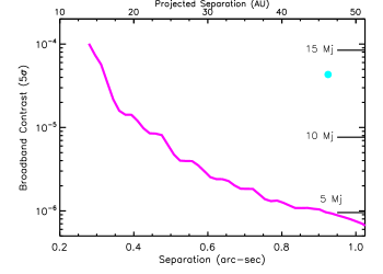
Figure 11: The 5-$\sigma$ broadband contrast curve for $\kappa$ And data reduced using ADI+SDI. A cyan circle identifies the position and contrast of $\kappa$ And b; horizontal bars denote the contrast for substellar objects of various masses.

Our data do not reveal any additional companions located interior to $\kappa$ And b. To set limits on companions located interior to $\kappa$ And b, we first divided the 5-$\sigma$ residual noise profile in the wavelength-collapsed ADI+SDI image by the median stellar flux. We injected model L0 $\gamma$ dwarf spectra from the Bonnefoy et al. (2014a) library and propagated them through ADI and then SDI to determine their signal loss. We performed ten iterations of forward-modeling and interpolated the results to create a “flat field” to correct our noise profile map. Due to CHARIS’s large bandpass and our use of local (subtraction zone) masking, signal loss from SDI was minor ($\lesssim$ 20%), and the radially-averaged throughput ranged between 59% and 73% from $\rho$ $\sim$ 0$\farcs$3 to 1$\farcs$0.

To translate our broadband contrast limits to stellar mass, we used the Baraffe et al. (2003) evolutionary models to predict values for gravity and temperature and then atmosphere models to determine the “broadband” (JHK) flux density for 3–30 $M_{\rm J}$ substellar objects at these gravities/temperatures at 40 $Myr$. Values ranged from $T_{\rm eff}$ $\sim$ 600 $K$, log(g) = 3.5 to $T_{\rm eff}$ $\sim$ 2300 $K$, log(g) = 4.5. Atmosphere models draw from A. Burrows, using cloud prescriptions that provide good fits to substellar objects covering most of this range: HR 8799 cde, $\beta$ Pic b, and ROXs 42Bb (Currie et al., 2011; Madhusudhan et al., 2011; Currie et al., 2013, Currie, Burrows et al. 2018 in prep.).

Figure 11 displays our contrast curve. The broadband contrast dips just below 10^-6 at wide separations and gradually increases to 10^-5 at $\rho$ $\sim$ 0$\farcs$35–0$\farcs$45. Despite extremely poor field rotation and $\sim$ 12 minutes of integration time, our contrasts exterior to 0$\farcs$35–0$\farcs$45 are comparable to those from SCExAO/HiCIAO for HD 36546 – a factor of 3 deeper and factor of 10 better field rotation (Currie et al., 2017a)– as well as Gemini Planet Imager first-light imaging of $\beta$ Pic b, which were likewise much deeper than our data (Macintosh et al., 2014). Companions with contrasts and masses at or below that of $\kappa$ And b would have been detectable down to 0$\farcs$3 (15 au). Any companion more massive than $\kappa$ And b and capable of scattering it to wide separations must lie within 15 au.

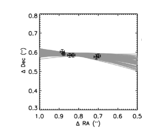
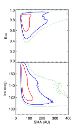
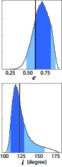
Figure 12: Orbit fitting results using OFTI (Blunt et al., 2017) and ExoSOFT (Mede and Brandt, 2017). (Left) The best-fit orbits from OFTI compared to astrometric data. The first two epochs draw from HiCIAO astrometry presented in Carson et al. (2013); the third, fourth, and last epochs are our NIRC2 astrometry while fifth epoch is from CHARIS. The results and the goodness-of-fits from ExoSOFT are comparable. (middle) The 68% (red) and 95% (blue) confidence intervals for semimajor axis, inclination, and eccentricity from OFTI. (right) The probability distributions for eccentricity and inclination from ExoSOFT: the dark and light blue regions identify the 68% and 95% confidence intervals, respectively.

Table 3: Orbit Fitting for $\kappa$ And b

		OFTI		ExoSOFT
Orbital Element	Unit	Median [68% C.I.]	[95% C.I.]	Median [68% C.I.]	[95% C.I.]
a	au	76.5 [56.7, 128.2]	[47.2, 286.6]	99.0 [53.7, 126.6]	[45.1, 216.1]
P	yr	399.9 [254.9, 868.1]	[193.3, 2899.5]	588.8 [214.1, 825.9]	[169.0, 1868.8]
e		0.80 [0.67, 0.87]	[0.54, 0.93]	0.69 [0.59,0.83]	[0.47, 0.90]
i	o	136.2 [119.6, 157.4]	[111.1, 171.5]	121.2 [109.2,129.2]	[105.5, 158.7]
$\omega$	o	126.5 [49.1, 161.0]	[3.6, 176.7]	129.5 [95.7, 157.2]	[71.1, 195.5]
$\Omega$	o	75.9 [54.1, 100.5]	[15.4, 162.1]	75.7 [64.1, 87.0]	[31.1, 113.4]
$T_{0}$	yr	2042.7 [2039.1, 2051.5]	[2037.3, 2062.7]	2047.62 [2038.38,2053.82]	[2036.14, 2069.47]

Note. — Orbits are fit to the four new NIRC2 and CHARIS astrometric points plus two HiCIAO epochs listed in Carson et al. (2013).

6 The Orbit of $\kappa$ And b

Well-calibrated astrometry for $\kappa$ And b now spans five years and reveals a clear change in position with time. Orbital solutions derived for objects with low phase coverage are highly sensitive to input priors on different orbital parameters (Kosmo OŃeil et al., 2018). We use two different approaches – OFTI and ExoSOFT (Blunt et al., 2017; Mede and Brandt, 2017) – and adopt different priors to determine plausible orbital properties of the companion. The first investigation of $\kappa$ And b’s orbit was carried out by Blunt et al. (2017); our focus is to improve upon these constraints using a longer time baseline to determine the companion’s orbital direction and identify plausible values for its semimajor axis, eccentricity, and orbital inclination.

OFTI uses a Bayesian rejection sampling algorithm to efficiently determine the most plausible orbital parameters. We assume Gaussian priors for the parallax centered on GAIA DR2 catalogue values, a uniform prior in stellar mass (2.7–2.9 $M_{\odot}$), and impose a log-normal prior in semimajor axis (a^-1). ExoSOFT uses a Markov Chain Monte Carlo approach to determine the orbital fit and posterior distributions and Simulated Annealing to find reasonable starting positions for the Markov chain and tune step sizes. We assume a Jeffrey’s prior for the semimajor axis (a^-1/ln(a_max/a_min)), which gives equal prior probability for the semimajor axis for each decade of parameter space explored. Our astrometric errors conservatively consider the intrinsic SNR of the detection, uncertainties in image registration, uncertainties due to self-subtraction/annealing, and absolute astrometric calibration.

Figure 12 shows orbital fits using OFTI and ExoSOFT and Table 3 lists the median value for orbital parameters and their 68% confidence intervals. Both approaches determine that $\kappa$ And b orbits clockwise on the plane of the sky, likely has a semimajor axis substantially larger than its projected separation (e.g. 76.5^o${}^{+51.7^{o}}_{-19.8^{o}}$ at the 68% confidence interval for OFTI) and is highly eccentric (e.g. $e$ $\sim$ 0.69${}^{+0.14}_{-0.10}$ for ExoSOFT), although astrometric offsets from different epochs can in principle mimic a non-zero eccentricity. OFTI finds a wide range of acceptable orbital inclinations – 119.6^o–157.4^o (111.1^o–171.5^o within the 95% confidence interval) – meaning that $\kappa$ And b’s orbit is likely inclined $\sim$ 30–70^o from face-on: a subset of these solutions could imply that the companion’s orbital plane is aligned with that of the star ($i_{eq}$ $\sim$ 60^o). ExoSOFT finds slightly lower inclinations although orbits aligned with the star’s rotational axis lie within the 95% confidence interval.

7 Discussion

Table 4: Properties of the $\kappa$ And system

Parameter	$\kappa$ And A	$\kappa$ And b	Reference
Object Properties
d (pc)	$50.0\pm 0.1$	…	1
Age (Myr)	$47^{+27}_{-40}$	$\approx$ $40^{+34}_{-19}$?	2, 6
Mass	2.8 $M_{\odot}$	$\approx$ 13${}^{+12}_{-2}$ $M_{\rm J}$?	2, 6
log(L/L⊙)	$1.80^{+1.7}_{-0.04}$	-3.81$\pm$ 0.05	2, 6
Spectral type	B9IV/B9V	L0-L1$\gamma$	2, 5, 6
$\mathrm{T_{eff}}$ (K)	$11327^{+421}_{-44}$	$1700-2000$	2, 6
log g (dex)	$4.174^{+0.019}_{-0.012}$	$\approx$ $4.0-4.5$?	2, 4
Photometry
J (mag)	$4.26\pm 0.04$	$15.84\pm 0.09$	2
H (mag)	$4.31\pm 0.05$	$15.01\pm 0.07$	2
$\mathrm{K_{s}}$ (mag)	$4.32\pm 0.05$	$14.37\pm 0.07$	2
L’ (mag)	$4.32\pm 0.05$	$13.12\pm 0.1$	3, 4
NB_4.05 (mag)	$4.32\pm 0.05$	$13.0\pm 0.2$	4
M’ (mag)	$4.30\pm 0.06$	$13.3\pm 0.3$	4
Astrometry
UT Date	Data Source	[E, N]″
2012 01 01.	AO188/HiCIAO	[0.884 $\pm$ 0.010, 0.603 $\pm$ 0.011]	3
2012 07 08	AO188/HiCIAO	[0.877 $\pm$ 0.007, 0.592 $\pm$ 0.007]	3
2012 11 03	Keck/NIRC2	[0.846 $\pm$ 0.010, 0.584 $\pm$ 0.010]	2
2013 08 18	Keck/NIRC2	[0.829 $\pm$ 0.010, 0.585 $\pm$ 0.010]	2
2017 09 05	SCExAO/CHARIS	[0.710 $\pm$ 0.012, 0.576 $\pm$ 0.012]	2
2017 12 09	Keck/NIRC2	[0.699 $\pm$ 0.010, 0.581 $\pm$ 0.010]	2

Note. — References – 1) Gaia Collaboration, 2) this work, 3) Carson et al. (2013), 4) Bonnefoy et al. (2014a), 5) Hinkley et al. (2013), 6) Jones et al. (2016). We conservatively assign a positional uncertainties in each coordinate to account for the difference between the apparent and actual position of the star underneath the coronagraph spot (NIRC2, $\sim$ 0.25 pixels) or from a polynominal fit to the apparent centroid positions derived from satellite spots (CHARIS, $\sim$ 0.25 pixels), uncertainties in the north position angle and pixel scale (larger for CHARIS), the intrinsic signal-to-noise (both), uncertainties in the parallactic angle as recorded in the first header (primarily NIRC2), and uncertainties in the astrometry due to self-subtraction/annealing (both, larger for NIRC2). The age, gravity, and mass are not directly measured, so we denote their estimates with a ”?”.

7.1 New Constraints on the Atmosphere and Orbit of $\kappa$ And b

Our study clarifies the atmospheric and orbital properties of $\kappa$ And b, summarized in Table 4. Previous studies analyzing broadband photometry and P1640 spectra (Bonnefoy et al., 2014a; Hinkley et al., 2013) admit a wide range of acceptable spectral types or different answers depending on a) whether field or low/intermediate gravity comparison spectra are used or b) the wavelength range used for matches with empirical spectra. Comparing the CHARIS spectra to both optically-anchored spectral templates and spectral libraries shows that $\kappa$ And b best resembles a young, low-gravity L0–L1 dwarf (L0–L1$\gamma$) like 2MASSJ0141-4633. Its $H$-band spectral shape in particular shows strong evidence for a low surface gravity.

A number of factors may explain why our conclusions about $\kappa$ And b’s spectrum show small differences with those presented in Hinkley et al. (2013). Chiefly, the signal-to-noise ratio of $\kappa$ And b’s spectrum is substantially higher (SNR_med.,CHARIS $\sim$ 20.5 vs. 5 for P1640), in large part owing to SCExAO’s extremely high-fidelity AO correction resulting in a deep raw contrast. This allowed us to extract a higher-fidelity spectrum and more clearly identify which spectral templates and empirical spectra match $\kappa$ And b. Furthermore, calibrating the $\kappa$ And b spectrum from P1640 data is arguably more challenging since it relies on forward-modeling data reduced using SDI only (see Pueyo, 2016). The slightly wider, redder bandpass (1.1–2.4 $\mu m$ vs. 0.9–1.8 $\mu m$) also probes more of $\kappa$ And b’s spectral energy distribution, also aiding the identification of the companion’s best-fit spectral properties. Appendix B identifies an additional possible source of differences from the template spectrum used for spectrophotometric calibration.

While Carson et al. (2013) demonstrated that $\kappa$ And b is a bound companion, their short ($\sim$ 0.75 year) astrometric baseline precluded a detailed understanding of the companion’s orbit, admitting a wide range of parameter space (Blunt et al., 2017). Our astrometry establishes a 5-year baseline and decisively determined $\kappa$ And b’s orbital direction (clockwise). Orbital fits from two separate but complementary codes show that the companion’s orbital plane is highly inclined relative to sky and possibly coplanar with the rotation axis of the star. Its eccentricity is likely substantial. The semimajor axis of $\kappa$ And b suggests that the companion may orbit at a significantly wider separation than previously thought. The companion’s orbit – including inclination and semimajor axis – can be better clarified by including new astrometric measurements and determining solutions assuming observable-based priors (Kosmo OŃeil et al., 2018).

7.2 $\kappa$ And b in Context: Constraints/Limits on Temperature, Age, Gravity, Mass, and Formation

While we reserve a detailed atmospheric modeling analysis of $\kappa$ And b for a future publication, we can use empirical comparisons to now quantitatively limit its temperature, revisit its age, and estimate its surface gravity and mass. Combining these results with new information on $\kappa$ And b’s orbit allows us to revisit a discussion of its plausible formation mechanisms.

Temperature – A subset of the substellar objects whose spectra best fit $\kappa$ And b have a temperature derived from atmospheric modeling (Bonnefoy et al., 2014b; Faherty et al., 2016). Conveniently, the best-fitting object – 2MASSJ0141-4633 – was analyzed in Bonnefoy et al. (2014a) using models incorporating cloud/atmospheric dust prescriptions that accurately reproduce young, early L dwarf spectrophotometry over 1–5 $\mu m$ (Daemgen et al., 2017, T. Currie et al. in prep.). Bonnefoy et al. (2014a) derive $T_{\rm eff}$ = 1800${}^{+200}_{-100}$ $K$. While models utilized to constrain temperature in Faherty et al. (2016) were limiting cases that more poorly fit young, early L dwarfs, the derived temperature estimate for 2MASSJ0141-4633 using these models is consistent (1899 $K$ $\pm$ 123 $K$). Temperatures for 2MASSJ0120-5200, 2MASSJ0241-5511 and 2MASSJ2322-6151B (all L1$\gamma$) are slightly lower, as expected, and consistent with the range of L0–L1$\gamma$ temperatures listed in Gonzales et al. (2018). Separately, temperatures for the closest-fitting field spectral type (L3) have a comparable range: (1800–1900 $K$; Stephens et al., 2009). Taken together, we estimate a temperature of 1700–2000 $K$ for $\kappa$ And b.

Age – While a qualitative assessment of “low gravity” generally means “young”, the mapping onto age may not be decisive. Specifically, it is not clear yet how systematically different substellar objects are in gravity class from $\sim$ 10 $Myr$ to 40 $Myr$ to 100 $Myr$, etc. and population studies may identify some overlap. Nevertheless, we can use properties of the best-fitting substellar objects coupled with system kinematics and interferometric measurements of the primary to determine whether multiple lines of evidence are consistent with the same likely age of the $\kappa$ And system.

According to the Bayesian analysis tool for identifying moving group members, Banyan-$\Sigma$ (Gagne et al., 2018a), four of the seven objects in Table 2 are bona fide, decisive members of Tuc-Hor ($>$ 99.7% membership probability), which has a Li-depletion age of 40${}^{+5}_{-19}$ Myr (Kraus et al., 2014). A fifth is a “likely” member of Tuc-Hor (53% probability) and sixth a possible member (25% probability). The other is a previously-identified candidate member of AB Dor (130–200 $Myr$) (Bell et al., 2015), where previous versions of Banyan (e.g. Banyan-II) estimated a far higher membership probability than does Banyan-$\Sigma$. Tuc-Hor is comparable in age to the Columba association (t $\approx$ 30–40 $Myr$; Zuckerman et al., 2011; Bell et al., 2015), as both groups’ pre-main sequences (luminosity vs. temperature) are nearly identical (Bell et al., 2015). While $\kappa$ And b’s proposed membership in Columba is highly suspect (Hinkley et al., 2013), using new GAIA-DR2 astrometry Banyan-$\Sigma$ still suggests it is a possible member (20% probability).

Thus, regardless of whether $\kappa$ Andromedae actually is a member of Columba, properties of both the primary and companion are consistent with what a system coeval with Columba should look like. Considering all lines of evidence together, we favor an age of 40${}^{+34}_{-19}$ $Myr$, where the upper and lower bounds are equated with the age upper bound for the primary and the lower bound for most best-fitting comparison spectra, respectively.

Gravity – While there are few direct anchors for surface gravity for young substellar objects (see Stassun et al., 2006, 2007; Canty et al., 2013, and T. Currie et al. 2018 in prep.), atmosphere/substellar evolution models can help identify plausible values for $\kappa$ And b. Although a small subset of best-fit models that reproduced 2MASSJ0141-4633’s spectrum in Bonnefoy et al. (2014b) had high surface gravities expected for field objects (log(g) $\sim$ 5–5.5), most had log(g) = 4.0 $\pm$ 0.5. Using the Baraffe et al. (2003) evolutionary models, this object, siblings in Tuc-Hor, and slightly younger (20 Myr-old) ones are predicted to have surface gravities on the order of log(g) $\sim$ 4.1–4.2, while those of comparable temperature near our preferred upper age limit of $\sim$ 74 $Myr$ should have log(g) $\sim$ 4.5. Surface gravities of log(g) $\sim$ 4–4.5 are therefore supported by a joint consideration of detailed atmosphere modeling of best-fitting spectra and predictions from evolutionary models covering $\kappa$ And’s most plausible age range so far.

Mass – Armed with a revised estimate for $\kappa$ And b’s spectral type, photometry, and the system’s distance, we calculate a bolometric luminosity of log(L/L_⊙) = -3.81 $\pm$ 0.06 using the bolometric correction obtained by Todorov et al. (2010) for 2MASSJ0141-4633. Luminosities for the best-fitting L dwarfs in Tuc-Hor are comparable to $\kappa$ And b or slightly higher by 0.25 dex (-3.55 to - 3.8). As their implied masses are 12–15 $M_{\rm J}$, if $\kappa$ And is coeval with Tuc-Hor then $\kappa$ And b is likely lower in mass. Considering the full range of favored system ages, $\kappa$ And b’s estimated mass is 13${}^{+12}_{-2}$ $M_{\rm J}$ and companion-to-primary mass ratio is $q$ $\sim$ 0.005${}^{+0.005}_{-0.001}$.

Formation – Our results provide new information helpful for assessing how $\kappa$ And b relates to bona fide planets detected by both indirect techniques and direct imaging and low-mass brown dwarfs. While the companion’s mass is near or may even exceed the deuterium-burning limit, the utility and physical basis of this IAU criterion or any other hard mass upper limit for a “planet” is unclear (Luhman, 2008). Alternate criteria focusing on the demographics of imaged companions – mass ratio and separation – may more clearly distinguish planets from brown dwarf companions (Kratter et al., 2010; Currie et al., 2011).

While the plausible mass ratios of $\kappa$ And b are intermediate between that of HR 8799 cde ($q$ $\sim$ 4.5$\times$10^-3) and ROXs 42Bb ($q$ $\sim$ 9$\times$10^-3), its orbital separation is likely larger than any HR 8799 planets, more comparable to HIP 65426 b and ROXs 42Bb (90–150 au; Chauvin et al., 2017; Currie et al., 2014a). Similar to $\kappa$ And b, no additional companions have been found at smaller separations around HIP 65426 or ROXs 42B (Chauvin et al., 2017; Bryan et al., 2016). Although core accretion struggles to form massive companions in situ beyond 50–100 au, disk instability may yet be a viable mechanism to account for $\kappa$ And b, HIP 65426 b, and ROXs 42Bb (e.g. Rafikov, 2005). At least some protoplanetary disks contain a significant amount of mass at 50–150 au-scale separations that could be (and perhaps have been) converted into massive companions via gravitational instability (e.g. Andrews and Williams, 2007; Isella et al., 2016), although direct imaging surveys show that superjovian-mass planets at these separations are rare (Nielsen et al., 2013; Brandt et al., 2014; Galicher et al., 2016).

7.3 Future Studies of $\kappa$ And b

Follow-up low-resolution CHARIS spectroscopy in individual passbands ($J$/$H$/$K$; $R$ $\sim$ 80) could better clarify $\kappa$ And b’s atmospheric properties. Gravity-sensitive indices $H$-cont and $H_{2}K$ approximated in this work could be more reliably determined; $J$ band potassium lines (K_I) could provide a third assessment of the companion’s gravity (Allers and Liu, 2013). An improved census of substellar objects with ages at or just greater than that of Columba/Tuc-Hor (40–100 $Myr$) aided by the identification of new moving groups (e.g. Gagne et al., 2018b) could better establish a context for $\kappa$ And b and how its spectrum compares to the full range of very low, low, and intermediate gravity objects. Ground-based broadband photometry can bracket CHARIS’s coverage and also better probe evidence for clouds and small atmospheric dust, while more precisely constraining the companion’s temperature (Currie et al., 2011, 2013; Daemgen et al., 2017). Thermal infrared observations with the James Webb Space Telescope could reveal and help begin to quantify the abundance of $CO$, $CH_{4}$, and CO₂ (Beichman and Greene, 2018).

Higher-resolution ($R$ $\sim$ 3000) integral field spectroscopy of $\kappa$ And b achievable with Keck/OSIRIS and later on the Thirty Meter Telescope with IRIS will provide a signficant advance in understanding $\kappa$ And b’s gravity, clouds, chemistry, and perhaps formation (Larkin et al., 2006, 2016; Wright et al., 2014). OSIRIS and IRIS spectra can measure narrow gravity-sensitive lines of iron and sodium (Allers and Liu, 2013). Fitting these spectra with sophisticated forward models or analyzing them atmospheric retrievals should also yield estimates for $CO$, $H_{2}O$, $CH_{4}$, and perhaps NH₃ abundances from resolved molecular line emission (Barman et al., 2015; Todorov et al., 2016). The carbon-to-oxygen ratio derived from these abundance estimates may provide insights into the formation environment of $\kappa$ And b and perhaps identifying with other directly-imaged planets (e.g. Barman et al., 2015).

Appendix A CHARIS Astrometric Calibration

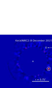
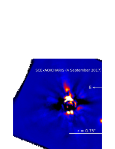
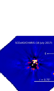
Figure 13: New HD 1160 data used for a preliminary CHARIS astrometric calibration: (left) Keck/NIRC2 from December 2017, (middle) SCExAO/CHARIS from 4 September 2017, and (right) SCExAO/CHARIS from 16 July 2017. Previously published SCExAO/CHARIS data from 6 September used in our calibration are shown in Currie et al. (2018).

While precise astrometric calibration is ongoing, in this paper we present a preliminary calibration tied to Keck/NIRC2 based on July 2017, September 2017, and December 2017 observations the HD 1160 system. HD 1160 has two wide (sub-)stellar companions (Nielsen et al., 2012), one of which (HD 1160 B) is near the edge of the CHARIS field of view at $\rho$ $\approx$ 0$\farcs$8. At a projected separation of $r$ $\sim$ 80 au, the low-mass companion HD 1160 B should not experience significant orbital motion (Nielsen et al., 2012; Garcia et al., 2017). Specifically, using the orbital fits from Blunt et al. (2017), the separation and position angle for HD 1160 B are expected to change by $\Delta$$\rho$ $\sim$ -0.27 mas $\pm$ 0.36 mas, $\Delta$PA $\sim$ 0.026^o $\pm$ 0.01^o between September and December 2017 and $\Delta$$\rho$ $\sim$ -0.41 mas $\pm$ 0.54 mas , $\Delta$PA $\sim$ 0.040^o $\pm$ 0.014^o between July and December 2017. At the separation of HD 1160 B a position angle change of 0.04^o is no greater than $\sim$ 5% of a NIRC2/CHARIS pixel: effectively HD 1160 B is stationary over this timeframe.

Keck/NIRC2 is precisely calibrated, with a north position angle uncertainty of 0.02^o and post-distortion corrected astrometric uncertainty of 0.5 mas (Service et al., 2016). Thus, we pinned the SCExAO/CHARIS astrometry for HD 1160 B to that for Keck/NIRC2 to calibrate CHARIS’s pixel scale and north position angle offset. This strategy follows that of the Gemini Planet Imager campaign team in using contemporaneous GPI and Keck/NIRC2 imaging of HR 8799 to fine-tune GPI’s astrometry (Konopacky et al., 2014).

Keck/NIRC2 $K$-band data for HD 1160 were obtained on UT 9 December 2017, immediately after $\kappa$ And, using the 0$\farcs$6 diameter partially transmissive coronagraphic spot. Images consist of 11 coadded covering roughly 5 degrees in parallactic angle motion. Basic NIRC2 data reduction procedures – flatfielding, dark subtraction, bad pixel mitigation, (post-rebuild) distortion correction, and image registration – follows the pipeline from Currie et al. (2011) previously used to process ground-based broadband data. HD 1160 B was visible in the raw data; no PSF methods were applied. However, the AO correction was modest and the star was blocked by coronagraph: we assumed a centroid uncertainty of 0.25 pixels in both directions. In determining the error budget, we also considered the intrinsic SNR of the detection.

The $JHK$ data for HD 1160 from SCExAO/CHARIS data for HD 1160 were previously reported in Currie et al. (2018), taken on 6 September 2017 in two sequences, one with the Lyot coronagraph and another using the shaped-pupil coronagraph with good AO performance. HD 1160 B is detected at a high significance in both data sets in all individual channels and data cubes, even without PSF subtraction techniques applied (SNR $\sim$ 100 in the wavelength-collapsed, sequence combined image). To the astrometry extracted from these data, we add astrometry determined from 4 September 2017 (obtained under extremely poor conditions) and 16 July 2017 (obtained under excellent conditions). Nominal astrometric errors consider the intrinsic SNR and a conservative estimate for the centroid (set to 0.25 pixels).

Table 5 shows our resulting astrometry for HD 1160 B; Figure 13 show images for NIRC2 data and previously unpublished SCExAO/CHARIS data. For the nominal CHARIS astrometric calibration (0$\farcs$0164 pixel^-1 and no north position angle offset), the CHARIS astrometry displays no significant astrometric deviation between data sets but is systematically offset from the Keck/NIRC2 astrometry. Taking uncertainty-weighted average astrometric offset, we obtain a revised pixel scale of 0$\farcs$0162 pixel^-1 $\pm$ 0$\farcs$0001 pixel^-1 and a north position angle offset of -2.20^o $\pm$ 0.27^o east of north (i.e. CHARIS data must be rotated an additional 2.2 degrees counterclockwise to achieve a north-up image).

Table 5: Preliminary SCExAO/CHARIS Astrometric Calibration

Telescope/Instrument (Coronagraph)	UT Date	$\rho_{nominal}$ (″)	PAnominal (o)	$\rho_{corr}$ (″)	PAcorr (o)
Keck/NIRC2 (Lyot)	9 December 2017	0.784 $\pm$ 0.006	244.93 $\pm$ 0.25	–	–
SCExAO/CHARIS (Lyot)	6 September 2017	0.797 $\pm$ 0.004	242.85 $\pm$ 0.15	0.785 $\pm$ 0.008	245.05 $\pm$ 0.27
SCExAO/CHARIS (SPC)	6 September 2017	0.796 $\pm$ 0.004	242.67 $\pm$ 0.13	0.784 $\pm$ 0.008	244.87 $\pm$ 0.26
SCExAO/CHARIS (Lyot)	4 September 2017	0.796 $\pm$ 0.005	242.60 $\pm$ 0.30	0.784 $\pm$ 0.009	244.80 $\pm$ 0.37
SCExAO/CHARIS (Lyot)	16 July 2017	0.796 $\pm$ 0.004	242.74 $\pm$ 0.15	0.784 $\pm$ 0.008	244.94 $\pm$ 0.27

Note. — Because our astrometric calibration is focused on the pixel scale and north position angle, we report astrometry in polar coordinates, rather than the usual rectangular coordinates. The astrometric errors consider variations in centroid measurement (e.g., a simple center-of-light calculation vs. gaussian fitting), the intrinsic signal-to-noise of the detection, and (for the CHARIS corrected astrometry) uncertainties in the absolute pixel scale and true north calibration.

Appendix B Absolute Spectrophotometric Calibration

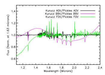
Figure 14: (left) Near-infrared spectra from the Pickles library (dashed lines) and from the Castelli and Kurucz (2004) atmosphere models (solid lines, offset by a constant). The spectra are normalized for each source at 1.63 $\mu m$ and compared to Vega’s spectrum. Despite being of a very similar temperature, the B9V Pickles models exhibits significant offsets that are not predicted by the Kurucz models and are larger than a photosphere (F0V) whose temperature ($\sim$ 7200 $K$; Currie et al., 2010; Pecaut et al., 2012) is significantly cooler. The Kurucz model spectra are nearly identical except at the shortest wavelengths for the coolest (F0V) model. (right) Ratio of the Kurucz to Pickles models for a given spectral type. At B9V, the Pickles models induce errors in spectrophotometric calibration up to 20%.

A key challenge with the new generation of coronagraphic extreme AO facilities is absolute spectrophotometric calibration. Unocculted images of the star are often unavailable and satellite spots of a known attenuation are used to estimate a planet-to-star contrast in each spectral channel. Absolute spectrophotometric calibration is necessary for accurate conclusions about any extracted planet/disk spectrum and requires an accurate model of the intrinsic spectrum of the unresolved target star (or a reference star) (e.g. Currie et al., 2017b).

The Pickles spectral library is the standard source for spectrophotometric calibration in the GPI Data Reduction Pipeline and has been used in direct imaging discovery and characterization papers (e.g. Macintosh et al., 2015). Importantly, it was used to calibrate P1640 spectra for $\kappa$ And b in Hinkley et al. (2013). However, we opted to use a robust, standard stellar atmosphere model (Castelli and Kurucz, 2004) instead. This is because we identified a potentially serious complication with multiple Pickles library entries at a level important for interpreting low-resolution planet/brown dwarf spectra..

Critically, Pickles et al. (1998) notes that near-infrared spectra is present for a few standard spectral types (e.g. A0V) but absent for the vast majority of their library, including the B9V spectral type. For spectral types lacking near-IR spectra, Pickles et al. uses “a smooth energy distribution” extending beyond the reddest available wavelength (typically 1.04 $\mu m$) to 5 $\mu m$ such that the integrated broadband photometry in major near-IR passbands match published values. However, this does not demonstrate that the spectral shape sampled at smaller $\Delta\lambda$ is consistent.

Figure 14 compares B9V and A0V Pickles spectra and counterparts from the Kurucz atmosphere models. The Pickles A0V, Kurucz A0V, and empirical Vega spectrum show strong agreement (left panel). The ratio of the Kurucz A0V to B9V spectrum over the CHARIS passbands is nearly constant, as expected for two objects with similar temperatures and similar exponential terms in their Planck functions (e.g. at $\lambda$ = [1.25, 2.15] $\mu m$ this ratio is [1.27, 1.22]) and a lack of broad molecular absorption features. Thus, we expect a very slowly changing or constant ratio of A0V/B9V over CHARIS passbands for the Pickles library spectra. However, as clearly shown in the right panel, the A0V/B9V flux ratio is unexpectedly variable over the CHARIS passbands, deviating by up to 20% compared to the Kurucz atmosphere models and simple predictions based on pure blackbody emission.

The practical consequence of using the Pickles B9V spectrum with extrapolated near-IR values instead of a stellar atmosphere model would be to suppress $\kappa$ And b’s signal at 1.4 $\mu m$ and the red edge of K and increase it at $\sim$ 1.7–1.8 $\mu m$. These wavelengths overlap with those sampled for gravity sensitive indices. Thus, it is possible that some of our different results for the nature of $\kappa$ And b vs. Hinkley et al. (2013) are due to issues with the Pickles B9V spectrum which have only now been highlighted. The choice of a proper stellar library may have important implications for interpreting substellar object spectra around other types of stars: for example, a $J$ spectrum extracted for a companion around an F0V star would deviate even more, perhaps leading to a misestimate of the companion’s temperature.

Appendix C A Generalized, Robust Forward-Modeling/Spectral Throughput Calibration Using (A-)LOCI

Powerful advanced least-squares PSF-subtraction algorithms like LOCI, KLIP, and derivatives can bias astrophysical signals, both reducing and changing the spatial distribution of the source intensity, thus affecting both spectophotometry and astrometry (e.g. Marois et al., 2010b; Pueyo et al., 2012a). The earliest attempts at correcting for this annealing focused on injecting synthetic point sources at a given separation but different position angles and then processing real data with these sources added in successive iterations to estimate throughput (e.g. Lafrenière et al., 2007). This approach yields a good estimate of the azimuthally-averaged point source throughput suitable for deriving contrast curves; however, it is computationally expensive (e.g. Brandt et al., 2013). Moreover, it is unsuitable for very precise spectrophotometry. This is because algorithm throughput can vary at different angles at a given separation if the intensity of the stellar halo has a high dynamic range (e.g., if it is “clumpy”), since high signal regions contribute more strongly to the residuals that the algorithm seeks to minimize (Marois et al., 2010a).

Forward-modeling provides a way to more accurately recover the intrinsic planet/disk brightness and astrometry/geometry, where the earliest methods focused on inserting negative copies of a planet PSF into the observing sequence with a brightness and position varied until it completely nulls the observed planet signal (Marois et al., 2010a; Lagrange et al., 2010). With the planet signal entirely removed from the reference library used in these algorithms, PSF subtracted images containing the planet signal have 100% throughput (Currie et al., 2014b). While robust, this method is also computationally expensive for integral field spectrograph data instead of single band photometry (i.e. the runtime is $n_{channels}$ more lengthy) or if the intensity distribution of the signal is unknown (e.g. a disk of some morphology) (Pueyo, 2016). To circumvent this problem, forward-modeling can be carried out in a more predictive fashion, where coefficients (for LOCI and derivatives) or Karhunen-Loève modes (for KLIP) used for PSF subtraction on science data are applied to empty images/data cubes containing only a synthetic planet or disk model (Soummer et al., 2012; Esposito et al., 2014; Pueyo et al., 2015; Currie et al., 2015a). However, if the planet/disk signal is contained in the reference library used for PSF subtraction, as is usually the case for ground-based imaging, the signal itself can perturb the KL modes/coefficients (Brandt et al., 2013; Pueyo, 2016). For KLIP, Pueyo (2016) developed a robust, generalized solution solving this problem, modeling the planet/disk signal as inducing a small perturbation on the KL modes.

Within the classic LOCI formalism, Brandt et al. (2013) thus far has developed the advanced approach most similar to that done by Pueyo (2016), efficiently modeling the planet as inducing a small perturbation on LOCI coefficients, $\boldsymbol{\beta}$. Their focus was an efficient and rapid computation of contrast curves for broadband data, not precise spectrophotometry/astrometry. In order to precompute the effective planet PSF inducing this perturbation, they therefore approximated it as a gaussian profile flanked by two sets of gaussian profiles at fixed position angle offsets and worked in the limiting case that the planet/disk intensity in the subtraction zone $I_{i,s}^{\prime}$ (not optimization zone) is far lower than the speckle intensity $I_{i,s}$. Absent this robust approach, several authors have introduced must incorporate modifications like local masking, a very large optimization zone, or an aggressive singular value cutoff (large $svd_{lim}$) to substantially reduce the influence of perturbations LOCI-like algorithms (e.g. Marois et al., 2010b; Currie et al., 2015a). However, we found that these modifications alone failed to yield a high-signal-to-noise spectrum for $\kappa$ And b whose throughput is precisely known.

Here, we develop a generalized forward-modeling solution in the (A-)LOCI formalism complementary to the KLIP forward-modeling approach in Pueyo (2016), adopting the formalism of and leveraging upon advances made by Brandt et al. (2013). In the standard case for LOCI-like algorithms, the set of coefficients $\alpha_{ij}$ applied to reference images $I_{j}$ determined from an optimization region $o$ minimize the subtraction residuals ${\cal R}_{i,o}^{2}$ over pixels $k$ for science image $I_{i}$:

$${\cal R}_{i,o}^{2}=\sum_{k}(I_{ik,o}-\sum_{j}\alpha_{ij}I_{jk,o}~{})^{2}.$$ (C1)

Following Brandt et al. (2013), we can perturb this equation by adding a planet PSF of signal $I^{\prime}$ to each reference image $j$ over pixels $k$, inducing a small perturbation in coefficients $\beta_{ij}$, thus the subtraction residuals are now:

$${\cal R}_{i,o}^{2}=\sum_{k}[I_{ik,o}+I_{ik,o}^{\prime}-\sum_{j}(\alpha_{ij}I_{j,o}+\alpha_{ij}I_{jk,o}^{\prime}+\beta_{ij}I_{jk,o}+\beta_{ij}I_{jk,o}^{\prime})~{}]^{2},$$ (C2)

Linearizing now around $\beta_{ij}$ instead of $\alpha_{ij}$, we find:

$$\frac{\partial{\cal R}_{i,o}^{2}}{\partial\beta_{il}}=0=\sum_{k}[(I_{lk,o}+I_{lk,o}^{\prime})(I_{ik,o}+I_{ik,o}^{\prime}-\sum_{j}(\alpha_{ij}I_{jk,o}+\alpha_{ij}I_{jk,o}^{\prime}+\beta_{ij}I_{jk,o}+\beta_{ij}I_{jk,o}^{\prime}))]$$ (C3)

Over the optimization zone $o$ (not the subtraction zone) and summed over pixels $k$, we assume that the speckle halo intensity is much larger than a planet ($I_{i,o}$ $>>$ $I_{i,o}^{\prime}$) and that the speckle halo subtracted by the reference library weighted by the nominal (A-)LOCI coefficients is zero ($I_{i,o}$ $-$ $\sum\limits_{j}(\alpha_{ij,o}I_{j,o}$) $\sim$ 0), reducing to a system of linear equations,

$$\sum_{k}I_{lk,o}(I_{ik,o}^{\prime}-\sum_{j}\alpha_{ij}I_{jk,o}^{\prime})=\sum_{j}\beta_{ij}\sum_{k}I_{lk,o}I_{jk,o},$$ (C4)

which can be solved by matrix inversion as done in Equation 4,

$$\boldsymbol{\beta}=(\mathbf{U}\mathbf{\Sigma_{>\mathit{svd_{lim}}}}\mathbf{V})^{-1}\cdot\mathbf{b^{\prime}},$$ (C5)

where U$\Sigma$V ($\boldsymbol{\rm A}$) is the same covariance matrix whose array elements are described in Equation 3 and $\boldsymbol{\rm b^{\prime}}$ is the column matrix describing how the effective (partially annealed) planet PSF induces a set of perturbation with coefficients $\boldsymbol{\rm\beta}$:

$${\rm b}_{l}^{\prime}=\sum_{k}I_{lk,o}(I_{ik,o}^{\prime}-\sum_{j}\alpha_{ij,o}I_{jk,o}^{\prime}).$$ (C6)

The residual emission of planet in frame $i$ within subtraction zone $s$ is then

$${\cal R}_{i,s}^{\prime}=\sum_{k}[I_{ik,s}^{\prime}-\sum_{j}(\alpha_{ij,o}I_{jk,s}^{\prime}+\beta_{ij,o}I_{jk,s}+\beta_{ij,o}I_{jk,s}^{\prime})].$$ (C7)

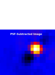
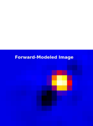
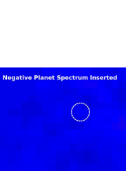
Figure 15: Demonstration of our spectrophotometric throughput correction using a combination of forward-modeling and iterative nulling. (left) The wavelength-collapsed PSF-subtracted image from Figure 1a showing clearly the signal peak from $\kappa$ And b and the negative subtraction footprints. (middle) The forward-modeled image at roughly the location of $\kappa$ And b predicted from perturbed A-LOCI coefficients and used to estimate the wavelength-dependent throughput correction for the companion’s spectrum. (right) The PSF-subtracted image after inserting a negative copy of $\kappa$ And b’s spectrum at the companion’s location into each data cube in our observing sequence. In all panels, the color stretch is the same and is in units of mJy (vertical bar). The negative spectrum - derived from forward-modeling - almost perfectly nulls the planet signal within one resolution element (dashed circle).

Throughout, we use the satellite spots to produce a model planet PSF for each channel. The empty data cubes containing the annealed planet PSF produced from the forward-model are then derotated and combined. Their photometry and astrometry are compared to input values to derive throughput for each spectral channel and astrometric offsets. These offsets were then applied to our spectral extraction subroutine to derive a flux-calibrated CHARIS spectrum. To confirm the validity of our forward-model, we inserted a negative copy of the extracted, corrected CHARIS spectrum into the real data at its predicted position in each data cube $\boldsymbol{x}$ – $I_{i,\lambda,neg.}=I_{i,\lambda}-I_{i,\lambda}^{\prime\prime}(\boldsymbol{x})$ – and slightly varied the position/brightness of the spectrum to verify that the forward-modeled solution is the correct one.

Figure 15 illustrates our forward-modeling method, demonstrating that the predicted annealed planet PSF matches the real one and the extracted CHARIS spectrum nulls the planet signal in the sequence-combined data cube. For our $\kappa$ And b data set using algorithm parameters adopted in §2. the spectrum throughput ranges between 77% and 92%; the astrometric offset is $\sim$ 0.2 pixels. In classic LOCI, very small optimization zones like those we adopt combined with poor field rotation can result in low throughput (Lafrenière et al., 2007). Our throughput is high and perturbations of the (A-)LOCI coefficients are low in large part because of local masking (see also Currie et al., 2013). This is because pixels corresponding to the subtraction zone $s$ (ostensibly containing most of the planet signal) are removed from the optimization zone $o$. Since the perturbed coefficients $\boldsymbol{\beta}$ are determined from a system of linear equations considering the optimization zone only, their values are much smaller when local masking is used. Truncating the covariance matrix A also reduces the algorithm aggressiveness and potentially the planet’s perturbations of (A-)LOCI coefficients.

This approach introduces some key modifications to that first proposed by Brandt et al. (2013) and utilized in the ACORNS pipeline. First, we explicitly calculate the effective planet PSF in each frame $i$ – $I_{ik,o}^{\prime}-\sum_{j}\alpha_{ij,o}$ – since the angular displacements of PSFs in frames $j$ and the coefficients $\alpha_{ij,o}$ are unique for each data set. Second, while we assumed that $I_{i,o}$ $>>$ $I_{i,o}^{\prime}$ to determine $\boldsymbol{\beta}$, the planet signal over the (typically much smaller) subtraction zone may not always be negligible in each spectral channel. Third, ACORNS (developed for low-Strehl data sets) modeled the planet PSF with a gaussian intensity distribution, whereas we use an empirical model unique for each data set. Fourth, it explicitly incorporates the distinction between optimization and subtraction zones and incorporates local masking and covariance matrix truncation, although ACORNS can easily be modified to do this as well.

Appendix D Extracted SCExAO/CHARIS Spectrum for $\kappa$ And b

We provide our extracted SCExAO/CHARIS spectrum for $\kappa$ And b in Table 6.

Table 6: SCExAO/CHARIS Spectrum in Flux Units (Observed)

Wavelength ($\mu m$)	Fν (mJy)	$\sigma$Fν (mJy)
1.1596	0.5910	0.0567
1.1997	0.6112	0.0529
1.2412	0.6942	0.0498
1.2842	0.8349	0.0487
1.3286	0.7658	0.0426
1.3746	0.2586	0.0403
1.4222	0.5371	0.0395
1.4714	0.5830	0.0393
1.5224	0.8103	0.0397
1.5750	0.8248	0.0405
1.6296	1.1274	0.0375
1.6860	1.2744	0.0351
1.7443	1.0190	0.0360
1.8047	0.8616	0.0310
1.8672	0.6344	0.0508
1.9318	0.9750	0.0429
1.9987	0.8215	0.0360
2.0678	1.0233	0.0338
2.1394	1.2442	0.0477
2.2135	1.3643	0.0492
2.2901	1.2739	0.0590
2.3693	1.2030	0.0832

Note. — Spectra are extracted from our conservative ADI/A-LOCI reduction and corrected for throughput losses. Measurements in regions with non-negligible telluric contamination and/or poor coverage from the template/empirical comparisons ($\lambda$ = 1.3746, 1.4222, 1.4714, 1.8672, 1.9318, and 1.9987 $\mu m$) were not used in our analysis.

References

- Allers and Liu (2013) Allers, K., Liu, M. C., 2013, ApJ, 772, 79
- Andrews and Williams (2007) Andrews, S. M., Williams, J. P., 2007, ApJ, 659, 705
- Artigau et al. (2010) Aritgau, E., Radigan, J., Folkes, S., et al., 2010, ApJ, 718, L38
- Baraffe et al. (2003) Baraffe, I., Chabrier, G., Barman, T. S., et al., 2003, A&A, 402, 701
- Barman et al. (2011) Barman, T. S., Macintosh, B., Konopacky, Q., Marois, C., 2011, ApJ, 735, L39
- Barman et al. (2015) Barman, T. S., Konopacky, Q., Macintosh, B., Marois, C., 2015, ApJ, 804, 61
- Beichman and Greene (2018) Beichman, C., A., Green, T. P., 2018, arxiv:803.03730
- Bejar et al. (2008) Bejar, V. J. S., Zapatero Osorio, M. R., Pérez-Garrido, A., et al., 2008, ApJ, 673, L105
- Bell et al. (2015) Bell, C., Mamajek, E. E., Naylor, T., 2015, MNRAS, 454, 593
- Blunt et al. (2017) Blunt, S., Nielsen, E., DeRosa, R., et al., 2017, AJ, 153, 229
- Bonnefoy et al. (2014a) Bonnefoy, M., Currie, T., Marleau, G.-D., et al., 2014, A&A, 562, 111
- Bonnefoy et al. (2014b) Bonnefoy, M., Chauvin, G., Lagrange, A.-M., et al., 2014, A&A, 562, 127
- Bonnefoy et al. (2016) Bonnefoy, M., Zurlo, A., Baudino, J.-L., et al., 2016, A&A, 587, 58
- Boss (1997) Boss, A., 1997, Science, 276, 1836
- Bowler and Hillenbrand (2015) Bowler, B. P., Hillenbrand, L. A., 2015, ApJ, 811, L30
- Brandt and Huang (2015) Brandt, T. D., Huang, C. X., 2015, ApJ, 807, 58
- Brandt et al. (2013) Brandt, T. D., McElwain, M., Turner, E. L., et al., 2013, ApJ, 764, 183
- Brandt et al. (2014) Brandt, T. D., McElwain, M., Turner, E. L., et al., 2014, ApJ, 794, 159
- Brandt et al. (2017) Brandt, T. D., Rizzo, M., Groff, T., et al., 2017, JATIS, 3, 8002
- Bryan et al. (2016) Bryan, M., Bowler, B. P., Knutson, H., et al., 2016, ApJ, 827, 100
- Burress et al. (2013) Burress, R., Hinkley, S., Wahl, M., et al., 2013, Proceedings of the Third AO4ELT Conference. Firenze, Italy, May 26-31, 2013, Eds.: Simone Esposito and Luca Fini Online at http://ao4elt3.sciencesconf.org/, id.52
- Burrows et al. (2006) Burrows, A., Sudarsky, D., Hubeny, I., 2006, ApJ, 640, 1063
- Canty et al. (2013) Canty, J. I., Lucas, P. W., Roche, P. F., Pinfield, D. J., 2013, MNRAS, 435, 2650
- Carson et al. (2013) Carson, J., Thalmann, C., Janson, M., et al., 2013, ApJ, 763, L32
- Castelli and Kurucz (2004) Castelli, F., Kurucz, R., 2004, arxiv preprints (astro-ph/0405087)
- Chauvin et al. (2017) Chauvin, G., Desidera, S.; Lagrange, A.-M, et al., 2017, A&A, 605, L9
- Chauvin et al. (2018) Chauvin, G., Gratton, R., Bonnefoy, M., et al., 2018, A&A in press, arxiv:1801.05850
- Chilcote et al. (2017) Chilcote, J., Pueyo, L., De Rosa, R., et al., 2017, AJ, 153, 182
- Cruz et al. (2018) Cruz, K., Nunez, A., Burgasser, A. J., et al., 2018, AJ, 155, 34
- Currie et al. (2010) Currie, T., Hernandez, J., Irwin, J., et al., 2010, ApJS, 186, 191
- Currie et al. (2011) Currie, T., Burrows, A., Itoh, Y., et al., 2011, ApJ, 729, 128
- Currie et al. (2012) Currie, T., Debes, J., Rodigas, T., et al., 2012, ApJ, 760, L32
- Currie et al. (2013) Currie, T., Burrows, A., Madhusudhan, N., et al., 2013, ApJ, 776, 15
- Currie et al. (2014a) Currie, T., Daemgen, Debes, J., et al., 2014a, ApJ, 780, L30
- Currie et al. (2014b) Currie, T., Burrows, A., Girard, J., et al., 2014b, ApJ, 795, 133
- Currie et al. (2014c) Currie, T., Muto, T., Kudo, T., et al., 2014c, ApJ, 796, L30
- Currie et al. (2015a) Currie, T., Cloutier, R., Brittain, S., 2015a, ApJ, 814, L7
- Currie et al. (2015b) Currie, T., Lisse, C., Kuchner, M., et al., 2015b, ApJ, 807, L7
- Currie et al. (2017a) Currie, T., Guyon, O., Tamura, M., et al., 2017, ApJ, 836, L15
- Currie et al. (2017b) Currie, T., Brittain, S., Grady, C., et al,. 2017, RNAAS, 1, 40
- Currie et al. (2018) Currie, T., Kasdin, N. J., Groff, T., et al., 2018, PASP, 130, 044505
- Cushing et al. (2005) Cushing, M. C., Rayner, J., Vacca, W., 2005, ApJ, 623, 1115
- Cushing et al. (2008) Cushing, M. C., Marley, M. S., Saumon, D., et al., 2008, ApJ, 678, 1372
- Daemgen et al. (2017) Daemgen, S., Todorov, K., Silva, J., et al., 2017, A&A, 601, 65
- David and Hillenbrand (2015) David, T. J., Hillenbrand, L. A., 2015, ApJ, 804, 146
- Delorme et al. (2012) Delorme, P., Gagne, J., Malo, L., et al., 2012, A&A, 548, 26
- Dupuy et al. (2018) Dupuy, T., Liu, M. C., Allers, K. N., et al., 2018, AJ, 156, 57
- Esposito et al. (2014) Esposito, T., Fitzgerald, M., Graham, J., Kalas, P., 2014, ApJ, 780, 25
- Faherty et al. (2016) Faherty, J. K., Riedel, A. C., Cruz, K. L., et al., 2016, ApJS, 225, 10
- Gagne et al. (2014) Gagne, J., Lafreniere, D., Duyon, R., et al., 2014, ApJ, 783, 121
- Gagne et al. (2015) Gagne, J., Faherty, J., Lafreniere, D., et al., 2015, ApJS, 219, 33
- Gagne et al. (2018a) Gagne, J., Mamajek, E., Malo, L., et al., 2018, ApJ, 856, 23
- Gagne et al. (2018b) Gagne, J., Faherty, J., Mamajek, E., 2018, ApJ, 865, 136
- Galicher et al. (2016) Galicher, R., Marois, C., Macintosh, B., et al,. 2016, A&A, 594, 63
- Garcia et al. (2017) Garcia, E. V., Currie, T., Guyon, O., et al., 2017, ApJ, 834, 162
- Golimowski et al. (2004) Golimowski, D., et al., 2004, AJ, 131, 3109
- Goebel et al. (2018) Goebel, S., Currie, T., Guyon, O., et al., 2018, AJ submitted
- Gonzales et al. (2018) Gonzales, E. C., Faherty, J. K., Gagne, J., et al., 2018, ApJ in press, arxiv.1807.04794
- Greco and Brandt (2016) Greco, J., Brandt, T. D., 2016, ApJ, 833, 134
- Groff et al (2013) Groff, T. D., Peters, M. A., Kasdin, N. J., 2013, SPIE, 8864, 0
- Groff et al. (2015) Groff, T. D., Kasdin, N. J., Limbach, M., et al., 2015, SPIE, 9605, 1
- Hinkley et al. (2013) Hinkley, S., et al., 2013, ApJ, 779, 153
- Isella et al. (2016) Isella, A., Guidi, G., Testi, L., et al., 2016, Phys. Rev. Lett., 117, 251101
- Jones et al. (2016) Jones, J., White, R. J., Quinn, S., et al., 2016, ApJ, 822, L3
- Jovanovic et al. (2015a) Jovanovic, N., Martinache, F., Guyon, O., et al., 2015, PASP, 127, 890
- Jovanovic et al. (2015b) Jovanovic, N., Guyon, O., Martinache, F., et al., 2015, ApJ, 813, L24
- Kenyon and Bromley (2009) Kenyon, S. J., Bromley, B., 2009, ApJ, 690, L140
- Keppler et al. (2018) Keppler, M., Benisty, M., Muller, A., et al., 2018, A&A in press, arxiv1806.11568
- Kirkpatrick et al. (2006) Kirkpatrick, J. D., Barman, T. S., Burgasser, A. J., et al., 2006, ApJ, 639, 1120
- Knapp et al. (2004) Knapp, G. R., Leggett, S. K., Fan, X., et al. 2004, AJ, 127, 3553
- Konopacky et al. (2014) Konopacky, Q., Thomas, S., Macintosh, B., et al., 2014, Proc. SPIE, 9147, 914784
- Kosmo OŃeil et al. (2018) Kosmo OŃeil, K., Martinez, G., Hees, A., et al., 2018, arxiv:809.05490
- Kratter et al. (2010) Kratter, K., Murray-Clay, R., Youdin, A., et al., 2010, ApJ, 710, 1375
- Kraus et al. (2014) Kraus, A., Shkolnik, E. L., Allers, K., Liu, M. C., 2014, AJ, 147, 146
- Kuhn et al. (2018) Kuhn, J., Serabyn, E., Lozi, J., et al., 2018, PASP, 130, 985
- Kuzuhara et al. (2013) Kuzuhara, M., Tamura, M., Kudo, T., et al., 2013, ApJ, 774, 11
- Lafrenière et al. (2007) Lafreniére, D., Marois, C., Duyon, R., et al., 2007, ApJ, 660, 770
- Lagrange et al. (2010) Lagrange, A.-M., et al., 2010, Science, 329, 57
- Lambrechts and Johansen (2012) Lambrechts, M., Johansen, A., 2012, A&A, 544, 32
- Larkin et al. (2006) Larkin, J., Barczys, M., Krabbe, A., et al., 2006, Proc. SPIE, 6269, 1
- Larkin et al. (2016) Larkin, J., Moore, A. M., Wright, S. A., 2016, Proc. SPIE, 9908, 1
- Luhman (2008) Luhman, K., 2008, Extreme Solar Systems, ASP Conference Series, Vol. 398, proceedings of the conference held 25-29 June, 2007, at Santorini Island, Greece. Edited by D. Fischer, F. A. Rasio, S. E. Thorsett, and A. Wolszczan, p.357
- Macintosh et al. (2014) Macintosh, B., Graham, J., Ingraham, P., et al., 2014, PNAS, 111, 35
- Macintosh et al. (2015) Macintosh, B., Graham, J. R., Ingraham, P., et al., 2015, Science, 350, 64
- Madhusudhan et al. (2011) Madhusudhan, N., Burrows, A., Currie, T., 2011, ApJ, 737, 34
- Marois et al. (2006) Marois, C., Lafreniére, D., Duyon, R., al., 2006, ApJ, 641, 556
- Marois et al. (2008) Marois, C., Macintosh, B., Barman, T., et al., 2008, Science, 322, 1348
- Marois et al. (2010a) Marois, C., Zuckerman, B., Konopacky, Q., et al., 2010a, Nature, 468, 1080
- Marois et al. (2010b) Marois, C., Macintosh, B., Veran, J.-P.., 2010b, SPIE, 7736, 52
- Mawet et al. (2014) Mawet, D., Milli, J., Wahhaj, Z., et al., 2014, ApJ, 792, 97
- Mede and Brandt (2017) Mede, K., Brandt, T. D., 2017, AJ, 153, 135
- Naud et al. (2014) Naud, M.-E., Aritgau, E., Malo, L., et al., 2014, ApJ, 787, 5
- Nielsen et al. (2012) Nielsen, E., Liu, M. C., Wahhaj, Z., et al., 2012, ApJ, 750, 53
- Nielsen et al. (2013) Nielsen, E., Liu, M. C., Wahhaj, Z., et al., 2013, ApJ, 776, 4
- Pecaut et al. (2012) Pecaut, M., Mamajek, E., Bubar, E., 2012, ApJ, 746, 154
- Perrin et al. (2014) Perrin, M., Maire, J., Ingraham, P., et al., 2014, SPIE, 9147, 3
- Peters et al. (2012) Peters, M., et al., 2012, SPIE, 8446, 7
- Pickles et al. (1998) Pickles, A., et al. 1998, PASP, 110, 749
- Pueyo et al. (2012a) Pueyo, L., Crepp, J. R., Vasisht, G., et al., 2012, ApJS, 199, 6
- Pueyo et al. (2015) Pueyo, L., Soummer, R., Hoffman, J., et al., 2015, ApJ, 803, 31
- Pueyo (2016) Pueyo, L., 2016, ApJ, 824, 114
- Quanz et al. (2013) Quanz, S., Meyer, M. R., Kenworthy, M., et al., 2013, ApJ, 766, L1
- Rafikov (2005) Rafikov, R. 2005, ApJ, 621, L69
- Rameau et al. (2013) Rameau, J., Chauvin, G., Lagrange, A.-M., et al., 2013, ApJ, 779, L26
- Rajan et al. (2017) Rajan, A., Rameau, J., De Rosa, R., et al., 2017, AJ, 154, 10
- Robert et al. (2016) Robert, J., Gagne, J., Artigau, E., et al., 2016, ApJ, 830, 144
- Rodigas et al. (2012) Rodigas, T. J., Hinz, P., Leisenring, J., et al., 2012, ApJ, 752, 57
- Savransky (2015) Savransky, D., 2015, ApJ, 800, 100
- Service et al. (2016) Service, M., Lu, J. R., Campbell, R., et al., 2016, PASP, 128, 5004
- Slesnick et al. (2004) Slesnick, C., Hillenbrand, L. A., Carpenter, J. M., 2004, ApJ, 610, 1045
- Soummer et al. (2012) Soummer, R., Pueyo, L., Larkin, J., 2012, ApJ, 755, L28
- Stassun et al. (2006) Stassun, K., Mathieu, R., Valenti, J. A., 2006, Nature, 440, 311
- Stassun et al. (2007) Stassun, K., Mathieu, R., Valenti, J. A., 2007, ApJ, 664, 1154
- Stephens et al. (2009) Stephens, D., Leggett, S. K., Cushing, M. C., et al,. 2009, ApJ, 702, 154
- Todorov et al. (2010) Todorov, K., Luhman, K. L., McLeod, B., 2010, ApJ, 714, L84
- Todorov et al. (2016) Todorov, K., Line, M., Pineda, J., et al., 2016, ApJ, 823, 14
- Wright et al. (2014) Wright, S. A., Larkin, J. E., Moore, A. M., et al., 2014, Proc. SPIE, 9147, 9
- Yelda et al. (2010) Yelda, S., et al., 2010, ApJ, 725, 331
- Zuckerman et al. (2011) Zuckerman, B., et al., 2011, ApJ, 732, 61