Green Bank Telescope Observations of ${}^{3}{\rm He}^{+}$: H ii Regions

Abstract

During the era of primordial nucleosynthesis the light elements ${}^{2}{\rm H}$, ${}^{3}{\rm He}$, ${}^{4}{\rm He}$, and ${}^{7}{\rm Li}$ were produced in significant amounts and these abundances have since been modified primarily by stars. Observations of ${}^{3}{\rm He}^{+}$ in H ii regions located throughout the Milky Way disk reveal very little variation in the ${}^{3}{\rm He}/{\rm H}$ abundance ratio—the “${}^{3}{\rm He}$ Plateau”—indicating that the net effect of ${}^{3}{\rm He}$ production in stars is negligible. This is in contrast to much higher ${}^{3}{\rm He}/{\rm H}$ abundance ratios found in some planetary nebulae. This discrepancy is known as the “${}^{3}{\rm He}$ Problem”. Stellar evolution models that include thermohaline mixing can resolve the ${}^{3}{\rm He}$ Problem by drastically reducing the net ${}^{3}{\rm He}$ production in most stars. These models predict a small negative ${}^{3}{\rm He}/{\rm H}$ abundance gradient across the Galactic disk. Here we use the Green Bank Telescope to observe ${}^{3}{\rm He}^{+}$ in five H ii regions with high accuracy to confirm the predictions of stellar and Galactic chemical evolution models that include thermohaline mixing. We detect ${}^{3}{\rm He}^{+}$ in all the sources and derive the ${}^{3}{\rm He}^{+}/{\rm H^{+}}$ abundance ratio using model H ii regions and the numerical radiative transfer code NEBULA. The over 35 radio recombination lines (RRLs) that are simultaneously observed, together with the ${}^{3}{\rm He}^{+}$ transition provide stringent constraints for these models. We apply an ionization correction using observations of ${}^{4}{\rm He}$ RRLs. We determine a ${}^{3}{\rm He}/{\rm H}$ abundance gradient as a function of Galactocentric radius of $-0.116\pm\ 0.022\,\times\,$$10^{-5}$ kpc^-1, consistent with stellar evolution models including thermohaline mixing that predict a small net contribution of ${}^{3}{\rm He}$ from solar mass stars.

1 The ${}^{3}{\rm He}$ Problem

Standard stellar evolution models predict the production of significant amounts of ${}^{3}{\rm He}$ in low-mass stars ($M<3$$\,M_{\odot}$), with peak abundances of ${}^{3}{\rm He/H}\sim\rm few\times 10^{-3}$ by number (Iben, 1967a, b; Rood, 1972). As the star ascends the red giant branch, the convective zone subsumes the enriched material which is expected to be expelled into the interstellar medium (ISM) via stellar winds and planetary nebulae (Rood et al., 1976; Vassiliadis & Wood, 1993; Dearborn et al., 1996; Weiss et al., 1996; Forestini & Charbonnel, 1997). Using yields from these standard stellar models, Rood et al. (1976) predicted present day abundances of ${}^{3}{\rm He/H}\sim 4\times 10^{-5}$ which they interpreted as stemming from more of a stellar than primordial origin.

Early measurements of ${}^{3}{\rm He}^{+}$ in Galactic H ii regions found large source-to-source variations, ${}^{3}{\rm He/H}=1-15\times 10^{-5}$, that were difficult to reconcile with Galactic chemical evolution (Rood et al., 1979, 1984; Bania et al., 1987; Balser et al., 1994). Deriving abundance ratios is a two-step process: (1) accurately measuring the spectral lines of interest; and (2) calculating the abundance ratio which may require a model of the source. Balser et al. (1999a) showed that the most accurate ${}^{3}{\rm He}/{\rm H}$ abundances could be determined from nebulae that are morphologically simple; that is, H ii regions with a homogeneous density. Using only these “simple” sources, Bania et al. (2002) found that the ${}^{3}{\rm He}/{\rm H}$ abundance was relatively constant across the Galactic disk revealing a “${}^{3}{\rm He}$ Plateau”. They suggested that the net production/destruction of ${}^{3}{\rm He}$ by stars is close to zero and that the ${}^{3}{\rm He}$ Plateau level corresponded to the primordial abundance produced during Big Bang Nucleosynthesis (BBN). This was later confirmed by combining results from the Wilkinson Microwave Anisotropy Probe (WMAP) with BBN models resulting in a primordial abundance of $(^{3}{\rm He/H})_{\rm p}=1.00\pm\ 0.07\times 10^{-5}$ (Romano et al., 2003; Cyburt et al., 2008).

Galactic chemical evolution (GCE) models assuming standard stellar yields predict significantly larger ${}^{3}{\rm He}/{\rm H}$ abundance ratios over the history of the Galaxy than are observed in H ii regions (Galli et al., 1995, 1997; Olive et al., 1995). The ${}^{3}{\rm He}/{\rm H}$ abundance ratio should increase with time and be higher in locations with more star formation. Most models therefore predict a negative ${}^{3}{\rm He}/{\rm H}$ radial abundance gradient within the Galactic disk since the star formation rate is higher in the central regions of the Milky Way. Thus the inner Galaxy should have substantially more stellar processing than the outer disk. Detection of ${}^{3}{\rm He}^{+}$ in a few planetary nebulae (PNe) yielded abundances of ${}^{3}{\rm He/H}\sim 10^{-3}$, consistent with standard stellar evolution theory (Rood et al., 1992; Balser et al., 1997, 2006). But the ${}^{3}{\rm He}$ Plateau revealed by H ii region observations is inconsistent with this picture. Moreover, in-situ measurements of the Jovian atmosphere with the Galileo probe yielded ${}^{3}{\rm He}/^{4}{\rm He}=1.66\pm 0.05\times 10^{-4}$ (Mahaffy et al., 1998). This corresponds to a protosolar abundance of ${}^{3}{\rm He/H}=1.5\pm 0.2\times 10^{-5}$, indicating very little production of ${}^{3}{\rm He}$ over the past 4.5$\,{\rm Gyr}$. These discrepancies are called the “The ${}^{3}{\rm He}$ Problem” (e.g., Galli et al., 1997).

Rood et al. (1984) suggested that some extra-mixing process may reduce the ${}^{3}{\rm He}$ abundance, and this might also explain the depletion of ${}^{7}{\rm Li}$ in main-sequence stars and the low ${}^{12}{\rm C}/^{13}{\rm C}$ abundance ratios in low-mass red giant branch (RGB) stars (also see Hogan, 1995; Charbonnel, 1995; Weiss et al., 1996). Sweigart & Mengel (1979) proposed that meridional circulation on the RGB could lead to reduced ${}^{12}{\rm C}/^{13}{\rm C}$ ratios in field stars. Boothroyd & Sackmann (1999) developed an “ad hoc” mixing mechanism in low-mass stars to further process ${}^{3}{\rm He}$. GCE models that included this extra-mixing in about 90% of low-mass stars were shown to be consistent with observations (Galli et al., 1997; Tosi, 1998; Palla et al., 2000; Chiappini et al., 2002). Zahn (1992) developed a more consistent theory including the interaction between meridional circulation and turbulence in rotating, non-magnetic stars. Charbonnel (1995) used this rotation-induced mixing and showed that this could explain the ${}^{12}{\rm C}/^{13}{\rm C}$, ${}^{7}{\rm Li}$, and ${}^{3}{\rm He}$ anomalies in RGB stars. Charbonnel et al. (1998) argued that this rotationally induced extra mixing occurs in low-mass stars above the luminosity function bump produced when the hydrogen burning shell crosses the chemical discontinuity left by the retreating convective envelope early in the RGB phase. Furthermore, about 96% of low-mass RGB field or cluster stars have anomalously low ${}^{12}{\rm C}/^{13}{\rm C}$ ratios (Charbonnel & Do Nascimento, 1998). Unfortunately, more realistic stellar evolution models that treat the transport of angular momentum by meridional circulation and shear turbulence self consistently do not produce enough mixing around the luminosity bump to account for the observed surface abundance variations (Palacios et al., 2006).

Eggleton et al. (2006) described another type of mixing that was important by modeling a red giant in three-dimensions, whereby the ${}^{3}{\rm He}$(${}^{3}{\rm He}$, 2p)${}^{4}{\rm He}$ reaction creates a molecular weight inversion. They interpreted this mixing as a Rayleigh-Taylor instability just above the hydrogen-burning shell. This convective instability occurs when heavier material lies above lighter material. In contrast, Charbonnel & Zahn (2007a) interpreted this mixing as a thermohaline instability, a double-diffusive instability, that occurs in oceans and is also called thermohaline convection (Stern, 1960). As the molecular weight gradient increases, the temperature has a stabilizing effect since the time scale for thermal diffusion is shorter than the time it takes for the material to mix. This analysis developed by Charbonnel & Zahn (2007a) explains the ${}^{12}{\rm C}/^{13}{\rm C}$ abundance anomalies on the RGB and the ${}^{3}{\rm He}$ abundance ratios observed in H ii regions (but also see Denissenkov, 2010; Denissenkov & Merryfield, 2011; Henkel et al., 2017). Currently, the best stellar evolutionary models that include both the thermohaline instability and rotation-induced mixing were developed for low and intermediate-mass stars (Charbonnel & Lagarde, 2010; Lagarde et al., 2011). Lagarde et al. (2012) used these yields together with GCE models to predict a modest enrichment of ${}^{3}{\rm He}$ with time and ${}^{3}{\rm He}/{\rm H}$ abundance ratios about a factor of two higher in the central regions of the Milky Way relative to the outer regions.

2 GBT Observations and Data Reduction

2.1 H ii Region Sample

Our goal is to derive accurate ${}^{3}{\rm He}/{\rm H}$ abundance ratios for a sub-set of our H ii region sources to confirm the slight radial ${}^{3}{\rm He}$ gradient predicted by Lagarde et al. (2012). H ii region models have shown that morphologically simple sources yield the most accurate ${}^{3}{\rm He}/{\rm H}$ abundance ratio determinations (Balser et al., 1999a; Bania et al., 2007). They are nebulae that are well approximated by a uniform density sphere. We therefore selected five H ii regions from the sample in Bania et al. (2002), a sample that was chosen to be morphologically simple, have relatively bright ${}^{3}{\rm He}^{+}$ lines, and are located over a range of Galactocentric radii. Table 1 summarizes this sample of H ii regions and lists the source name, equatorial coordinates, local standard of rest (LSR) velocity, $V_{\rm LSR}$, Heliocentric distance, $D_{\rm sun}$, and Galactocentric radius, $R_{\rm gal}$.

Table 1: Galactic H ii Region Properties

	R.A. (J2000)	Decl. (J2000)	$V_{\rm LSR}$	$D_{\rm sun}$	$R_{\rm gal}$
Source	(hh:mm:ss.ss)	(dd:mm:ss)	($\,{\rm km\,s^{-1}}$)	(kpc)	(kpc)
S206	04:03:15.87	$+$51:18:54	$-$25.4	3.3	11.5
S209	04:11:06.74	$+$51:09:44	$-$49.3	8.2	16.2
M16	18:18:52.65	$-$13:50:05	$+$26.3	2.0	6.6
G29.9	18:46:09.28	$-$02:41:47	$+$96.7	5.8	4.4
NGC 7538	23:13:32.05	$+$61:30:12	$-$59.9	2.8	9.9

2.2 Data Acquisition

We made observations of the ${}^{3}{\rm He}^{+}$ spectral transition with the Green Bank Telescope (GBT) at X-band (8-10$\,{\rm GHz}$) between 2012 March 02 and 2012 August 10 (GBT/12A-114). The GBT half-power beam-width (HPBW) is 87″ at the ${}^{3}{\rm He}^{+}$ spectral transition frequency of 8665.65$\,{\rm MHz}$. We employ total power position switching by observing an Off position for 6 minutes and then the target (On) position for 6 minutes, for a total time of 12 minutes. The Off position is offset 6 minutes in R.A. relative to the On position so that the telescope tracks the same sky path. The GBT auto-correlation spectrometer (ACS) is configured with 8 spectral windows (SPWs) at two orthogonal, circular polarizations for a total of 16 SPWs. Each SPW had a bandwidth of 50$\,{\rm MHz}$ and a spectral resolution of 12.2$\,{\rm kHz}$, or a velocity resolution of 0.42$\,{\rm km\,s^{-1}}$ at 8665.65$\,{\rm MHz}$. Thus each total power On/Off pair consists of 16 independent spectra. We placed the ${}^{3}{\rm He}^{+}$ transition in 8 SPWs (4 tunings at 2 polarizations) with center frequencies: 8665.3, 8662.3, 8659.3, and 8656.3$\,{\rm MHz}$. The ${}^{3}{\rm He}^{+}$ line was thus shifted by 3$\,{\rm MHz}$ in each tuning. The goal is to reduce spectral baseline structure by averaging the four spectra since the detailed baseline structure is a function of the center frequency (see §2.4 for details). We also tuned to various RRLs by centering the remaining SPWs to 8586.56, 8440.0, 8918.0, and 8474.0$\,{\rm MHz}$. This tuning strategy includes a series of high-order RRLs (e.g., Hn$\alpha$, Hn$\beta$, Hn$\gamma$, etc.) that can be used to monitor system performance and to constrain H ii region models. It also includes adjacent RRLs (e.g., H114$\beta$ and H115$\beta$) for redundancy.

Project GBT/12A-114, consisting of 93 observing sessions, was designed to be a filler project where scheduling blocks of a few hours could be efficiently used at 9$\,{\rm GHz}$ to accumulate the integration time needed to detect the weak ${}^{3}{\rm He}^{+}$ transition with a good signal-to-noise ratio (SNR). The observations were performed by the GBT operators and inspected by the authors within days of the observations. The pointing and focus were updated every 2 hr by observing a calibrator located within 15$\,{}^{\circ}$ of the target position. Noise was injected into the signal path with an intensity of 5-10% of the total system temperature ($T_{\rm sys}$) to calibrate the intensity scale. For the GBT X-band system the noise diodes are $T_{\rm cal}\sim 2$$\,{\rm K}$. We observed the flux density calibrator 3C286 using the digital continuum receiver (DCR) to check the flux density calibration. We use the Peng et al. (2000) flux densities for 3C286 and assume a telescope gain of $2\,{\rm K}\,{\rm Jy}^{-1}$ (Ghigo et al., 2001). We deem the intensity scale to be accurate to within 5-10%.

2.3 Data Reduction and Analysis

The data were reduced and analyzed using the single-dish software package TMBIDL (Bania et al., 2016). Each spectrum was visually inspected and discarded if significant spectral baseline structure or radio frequency interference (RFI) was present. Narrow band RFI that did not contaminate the spectral lines was excised and included in the average. Spectra were averaged in a hierarchical way to assess any problems with the spectral baselines. For example, we performed the following tests: (1) inspected the average spectrum for each observing epoch to search for any anomalies; (2) divided the entire data set into several groups to make sure the noise was integrating down as expected; (3) compared the two orthogonal polarizations which should be similar; and (4) compared the different ${}^{3}{\rm He}^{+}$ SPWs.

Each SPW was divided into sub-bands with bandwidths between 10-25$\,{\rm MHz}$ to better fit the spectral baselines and to directly compare with H ii region models. Table 2 lists the properties of the 8 distinct sub-bands. The main spectral transition is given together with the center frequency, bandwidth, and all the other transitions within the sub-band. The spectral baseline was modeled by fitting a polynomial, typically of order 3-5, to subtract any sky continuum emission or baseline structure from the spectrum. Each spectrum was smoothed to a velocity resolution of 3$\,{\rm km\,s^{-1}}$. Spectral line profiles were fit by a Gaussian function using a Levenberg-Markwardt (Markwardt, 2009) least squares method to derive the peak intensity, the full-width at half-maximum (FWHM) line width, and the LSR velocity.

Table 2: Spectra Line Sub-bands

Main	Rest Freq.	Bandwidth
Transition	(MHz)	(MHz)	Other Transitions
${}^{3}{\rm He}^{+}$	8665.65	15.0	H171$\eta$, H213$\xi$, H222$\pi$
H91$\alpha$	8584.82	20.0	H154$\epsilon$, H179$\theta$, H198$\lambda$, H227$\rho$, H231$\sigma$, H249$\psi$
H114$\beta$	8649.10	15.0	H203$\mu$, H238$\nu$, H245$\chi$
H115$\beta$	8427.32	25.0	H155$\epsilon$, H187$\iota$, H210$\nu$, H215$\xi$
H130$\gamma$	8678.12	10.0	H208$\nu$, H234$\tau$
H131$\gamma$	8483.08	25.0	H164$\zeta$, H193$\kappa$, H199$\lambda$, H228$\rho$, H232$\sigma$, H236$\tau$
H144$\delta$	8455.38	10.0	H180$\theta$, H247$\chi$
H152$\epsilon$	8920.33	15.0	H206$\nu$, H224$\rho$, H228$\sigma$, H239$\phi$

2.4 Spectral Baseline Structure

The limiting factor in the spectral sensitivity of most single-dish telescopes is instrumental baseline structure caused primarily by reflections from the super structure (e.g, secondary focus, feed legs, etc.) that produce standing waves within the spectrum. The properties of these standing waves are a function of the total system noise and frequency and thus they are difficult to model. Balser et al. (1994) showed that since the phase of the standing waves depends on the sky frequency, averaging observations of the target over different observing seasons will reduce, but not eliminate, these baseline effects. This is because the Earth’s orbital motion shifts the observed sky frequency and, thus, the phase of the standing waves.

The GBT was specifically designed with a clear aperture to significantly reduce reflections from the secondary structure and therefore improve the image fidelity and spectral sensitivity. Nevertheless, baseline structure still, unfortunately, exists and is primarily located within the electronics (Fisher et al., 2003). The GBT X-band receiver is a heterodyne receiver wherein radio waves from the sky are mixed with a local oscillator (LO) to convert the signal to an intermediate frequency (IF). Unfortunately, the GBT IF system contains analog signals over a long path length, $\sim 1\,$mile, and across many electronic components that can produce reflections and, therefore, standing waves. The spectral baselines are significantly better for the GBT than for traditionally designed, on-axis telescopes but they are still the limiting factor in measuring accurate line parameters for weak, broad spectral lines.

Using a strategy similar to Balser et al. (1994), we simultaneously observed the ${}^{3}{\rm He}^{+}$ line in four SPWs, shifting the center sky frequency relative to the center IF frequency by 3, 6, and 9$\,{\rm MHz}$. The goal was to reduce the baseline structure by averaging these four SPWs. To test the efficacy of this approach, we observed two calibrators 3C 286 and 3C 84 with 9$\,{\rm GHz}$ flux densities of $\sim 5$ Jy and 25 Jy, respectively. The telescope gain is $2\,{\rm K}\,{\rm Jy}^{-1}$, so these flux densities correspond to continuum antenna temperatures of $T_{\rm c}=10$$\,{\rm K}$ and 50$\,{\rm K}$, respectively. N.B., we chose these bright calibrators to amplify any instrumental spectral artifacts and therefore the baseline structure is worse than in our target sources which have continuum antenna temperatures ${\it<10\,}$K. The observing procedures and ACS configuration were the same as the target observations. The advantage of using these extragalactic sources is that they do not have any measurable spectral lines at these frequencies and have a relatively flat spectrum across the 50$\,{\rm MHz}$ bandwidth.

The results are shown in Figure 1 for 3C 286 and Figure 2 for 3C 84. Data were averaged over several observing sessions for each of the ${}^{3}{\rm He}^{+}$ SPWs separately (left panels). We fit a polynomial with order 1 to each spectrum to remove any slope or intensity offset from the spectrum. These four spectra were shifted to align them in frequency and then averaged (right panels). Both circular polarizations are shown separately. The baseline structure is clearly different for each ${}^{3}{\rm He}^{+}$ SPW and between the orthogonal polarizations. The averaged spectrum is clearly flatter. Furthermore, the amplitude of the baseline features roughly scales with continuum intensity (c.f., Figure 1 versus Figure 2). The root-mean-square (rms) noise across 3C84 spectra is about 7 times larger than for 3C286 spectra. Averaging over the four ${}^{3}{\rm He}^{+}$ SPWs does not reduce the random (thermal) noise because the signals are correlated, but the instrumental (systematic) noise is reduced.

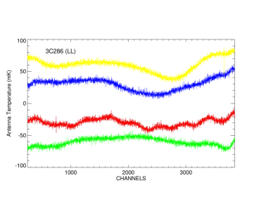
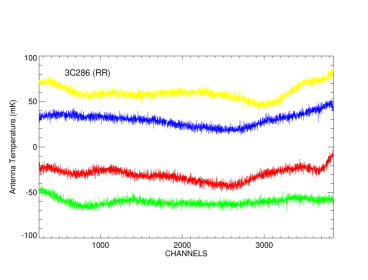
Figure 1: 3C 286 spectra where the antenna temperature is plotted as a function of channel number. The spectra have been offset for clarity. There are 4096 channels across a 50$\,{\rm MHz}$ bandwidth. A linear baseline was removed from each spectrum. Left Panel: All four ${}^{3}{\rm He}^{+}$ SPW spectra are shown as different colors for LL (top) and RR (bottom) circular polarizations. The sky frequency is shifted by 3, 6, and 9$\,{\rm MHz}$ (or 245, 490, and 735 channels) for each consecutive spectrum. Right Panel: The average ${}^{3}{\rm He}^{+}$ spectrum for LL (top) and RR (bottom) circular polarizations. The spectra were shifted to align them in frequency before averaging and therefore fewer channels are shown.

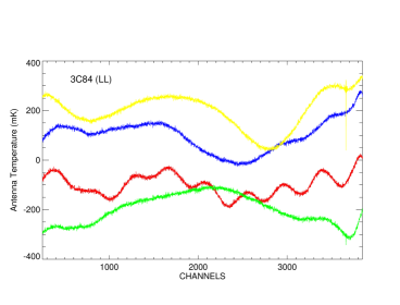
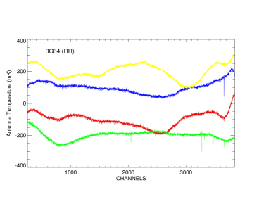
Figure 2: 3C 84 spectra where the antenna temperature is plotted as a function of channel number. See Figure 1 for details. The spectral baseline frequency structure seen in the left panels scales roughly with source continuum intensity. The 3C 84 continuum intensity is 5 times that of 3C 286 and the rms noise for 3C 84 is about 7 times larger than that of 3C 286.

3 ${}^{3}{\rm He}$ Abundances

For each source we generate spectra for all 8 sub-bands using the procedures discussed in §2, and perform the analyses described in §2.3 for the ${}^{3}{\rm He}^{+}$ transition. Table 3 summarizes the results. Listed are the source name, the Gaussian fit parameters and their associated 1-$\sigma$ errors, the rms noise in the line-free region, and the integration time. The Gaussian fits give the peak antenna temperature, the FWHM line width, and the LSR center velocity. The quantity of interest, however, is the ${}^{3}{\rm He}/{\rm H}$ abundance ratio by number. That is, to compare our results with theory we need to derive the abundance of ${}^{3}{\rm He}$ relative to H. This requires a model since the ${}^{3}{\rm He}^{+}$ hyperfine line intensity depends on the ${}^{3}{\rm He}^{+}$ column density, whereas both the free-free continuum and H RRL intensities depend on the emission measure or the integral of the density squared. The free-free thermal continuum intensity is used to derive the H abundance and so is a critical step in the derivation of the ${}^{3}{\rm He}/{\rm H}$ abundance ratio. We must also account for any neutral helium within the H ii region; that is, an ionization correction is necessary to convert the ${}^{3}{\rm He}^{+}/{\rm H^{+}}$ to a ${}^{3}{\rm He}/{\rm H}$ abundance ratio by number.

Table 3: ${}^{3}{\rm He}^{+}$ Spectral Line Parameters

	$T_{\rm L}$	$\sigma\,T_{\rm L}$	$\Delta{V}$	$\sigma\,\Delta{V}$	$V_{\rm LSR}$	$\sigma\,V_{\rm LSR}$	rms	$t_{\rm intg}$
Source	(mK)	(mK)	($\,{\rm km\,s^{-1}}$)	($\,{\rm km\,s^{-1}}$)	($\,{\rm km\,s^{-1}}$)	($\,{\rm km\,s^{-1}}$)	(mK)	(hr)
S206	3.796	0.076	20.88	0.55	$-25.37$	0.21	0.25	91.81
S209	1.963	0.147	22.40	1.94	$-50.83$	0.83	0.46	25.64
M16	4.749	0.150	18.63	0.90	$+27.21$	0.35	0.89	7.04
G29.9	4.843	0.092	27.31	0.93	$+98.64$	0.38	0.49	44.75
NGC 7538	3.814	0.190	25.90	1.80	$-61.83$	0.69	0.51	98.21

Here we use the numerical program NEBULA (Balser & Bania, 2018) to perform the radiative transfer of the ${}^{3}{\rm He}^{+}$ line, RRLs, and the free-free continuum emission through a model nebula. A detailed description of NEBULA is given in Balser (1995). Briefly, the model nebula is composed of only H and He within a three-dimension Cartesian grid with arbitrary density, temperature, and ionization structure. Each numerical cell consists of the following quantities: electron temperature, $T_{\rm e}$, electron density, $n_{\rm e}$, ${}^{4}{\rm He}^{+}/{\rm H^{+}}$ abundance ratio, ${}^{4}{\rm He}^{++}/{\rm H^{+}}$ abundance ratio, and the ${}^{3}{\rm He}^{+}/{\rm H^{+}}$ abundance ratio. Here we assume ${}^{4}{\rm He}^{++}/{\rm H^{+}}$ = 0.0 for all sources since the radiation field in Galactic H ii regions is not hard enough to doubly ionize He.

The radiative transfer is performed from the back of the grid to the front to produce the brightness distribution on the sky. To simulate an observation NEBULA calculates model spectra by convolving the brightness distribution with a Gaussian beam by the GBT’s HPBW at the ${}^{3}{\rm He}^{+}$ frequency. The ${}^{3}{\rm He}^{+}$ line is assumed to be in local thermodynamic equilibrium (LTE), but non-LTE effects and pressure broadening from electron impacts can be included for the RRLs. All spectra are broadened by thermal and microturbulent motions. In practice, each H ii region is modeled as a set of compact, uniform spheres constrained by Very Large Array (VLA) continuum images surrounded by a single halo component constrained by 140 Foot telescope continuum data to account for the total flux density (e.g., see Balser et al., 1995, 1999a). Additional, small scale structure is modeled by introducing a filling factor where gas is moved into higher density, small-scale clumps with no gas between clumps.

Table 4 summarizes the adopted NEBULA models for each source. Detailed information is given for each spherical, homogeneous component that includes the J2000 position, the linear size or diameter, $D$, the electron temperature, $T_{\rm e}$, the electron density, $n_{\rm e}$, the ${}^{4}{\rm He}^{+}/{\rm H^{+}}$ and ${}^{3}{\rm He}^{+}/{\rm H^{+}}$ abundance ratios by number, and the filling factor. The last component listed for each source is the halo component.

Table 4: H ii Region Models

	R.A.	decl.	$D$	$T_{\rm e}$	$n_{\rm e}$			Filling
	(J2000)	(J2000)	(pc)	($\,{\rm K}$)	($\,{\rm cm^{-3}}$)	${}^{4}{\rm He}^{+}/{\rm H^{+}}$	${}^{3}{\rm He}^{+}/{\rm H^{+}}$	Factor
S206
A	04:03:13.867	$+$51:18:32.02	0.865	9000	$5.498\times 10^{2}$	0.085	$1.89\times 10^{-5}$	1.00
B	04:03:13.753	$+$51:18:59.40	1.604	9000	$3.129\times 10^{2}$	0.085	$1.89\times 10^{-5}$	1.00
C	04:03:22.022	$+$51:17:39.26	0.902	9000	$2.742\times 10^{2}$	0.085	$1.89\times 10^{-5}$	1.00
D	04:03:19.237	$+$51:18:03.70	1.097	9000	$2.575\times 10^{2}$	0.085	$1.89\times 10^{-5}$	1.00
E	04:03:14.336	$+$51:18:05.08	1.166	9000	$2.474\times 10^{2}$	0.085	$1.89\times 10^{-5}$	1.00
Halo	04:03:15.870	$+$51:18:54.00	6.025	9000	$6.500\times 10^{1}$	0.085	$1.89\times 10^{-5}$	1.00
S209
A	04:11:06.133	$+$51:10:13.22	2.567	10500	$3.330\times 10^{2}$	0.070	$1.00\times 10^{-5}$	1.00
B	04:11:05.656	$+$51:09:31.09	3.395	10500	$2.065\times 10^{2}$	0.070	$1.00\times 10^{-5}$	1.00
C	04:11:08.602	$+$51:10:34.67	3.747	10500	$1.965\times 10^{2}$	0.070	$1.00\times 10^{-5}$	1.00
D	04:11:08.931	$+$51:08:57.27	3.063	10500	$1.668\times 10^{2}$	0.070	$1.00\times 10^{-5}$	1.00
Halo	04:11:06.740	$+$51:09:44.00	15.084	10500	$1.200\times 10^{1}$	0.070	$1.00\times 10^{-5}$	1.00
M16
A	18:18:50.252	$-$13:48:50.39	0.308	6000	$5.839\times 10^{2}$	0.080	$1.95\times 10^{-5}$	1.00
B	18:18:53.671	$-$13:49:37.35	0.336	6000	$4.408\times 10^{2}$	0.080	$1.95\times 10^{-5}$	1.00
C	18:18:53.666	$-$13:49:57.76	0.392	6000	$3.615\times 10^{2}$	0.080	$1.95\times 10^{-5}$	1.00
D	18:18:55.543	$-$13:51:47.90	0.315	6000	$4.413\times 10^{2}$	0.080	$1.95\times 10^{-5}$	1.00
Halo	18:18:52.650	$-$13:50:05.00	8.680	6000	$8.125\times 10^{1}$	0.080	$1.95\times 10^{-5}$	1.00
G29.9
A	18:46:09.470	$-$02.41.23.75	1.656	6500	$4.801\times 10^{2}$	0.070	$1.60\times 10^{-5}$	0.01
B	18:46:10.880	$-$02.41.58.91	1.469	6500	$4.409\times 10^{2}$	0.070	$1.60\times 10^{-5}$	0.01
Halo	18:46:09.280	$-$02:41:47.00	10.070	6500	$1.100\times 10^{2}$	0.070	$1.60\times 10^{-5}$	1.00
NGC 7538
A	23:13:30.694	$+$61:30:03.31	1.025	8000	$9.580\times 10^{2}$	0.083	$1.86\times 10^{-5}$	0.15
B	23:13:45.439	$+$61:28:19.51	0.196	8000	$4.009\times 10^{3}$	0.083	$1.86\times 10^{-5}$	0.15
C	23:13:30.663	$+$61:29:30.14	1.144	8000	$6.419\times 10^{2}$	0.083	$1.86\times 10^{-5}$	0.15
D	23:13:37.894	$+$61:29:13.57	0.949	8000	$5.807\times 10^{2}$	0.083	$1.86\times 10^{-5}$	0.15
Halo	23:13:32.050	$+$61:30:12.00	3.767	8000	$1.660\times 10^{2}$	0.083	$1.86\times 10^{-5}$	1.00

These H ii region NEBULA models are constrained using the following procedure:

1. Calculate ${\bf T}_{\bf\rm e}$. Use the single-dish H91$\alpha$ line-to-continuum ratio to calculate $T_{\rm e}$ assuming an optically thin nebula in LTE. Any non-LTE effects, including pressure broadening, should be small for the H91$\alpha$ RRL in H ii regions (see Shaver, 1980a, b). Assume a constant electron temperature for all components.

2. Calculate ⁴He⁺/H⁺. Use the line areas of the He91$\alpha$ and H91$\alpha$ RRLs to calculate the ${}^{4}{\rm He}^{+}/{\rm H^{+}}$ abundance ratio (e.g., Bania et al., 2007). Assume a constant ${}^{4}{\rm He}^{+}/{\rm H^{+}}$ abundance ratio for all components.

3. Model density structure. Use high spatial resolution continuum images (e.g., VLA data) near the ${}^{3}{\rm He}^{+}$ frequency to model the density structure assuming spherical, homogeneous spheres (e.g., Balser, 1995). This provides values for $n_{\rm e}$ and $D$ given $T_{\rm e}$, ${}^{4}{\rm He}^{+}/{\rm H^{+}}$, and $D_{\rm sun}$. Since H ii regions are typically resolved, use single-dish data to model any missing flux by assuming the missing emission is produced by a spherical, homogeneous halo.

4. Constrain halo density. Use NEBULA to generate the RRL brightness distributions on the sky, convolved with the GBT HPBW. Assume LTE with no pressure broadening. If necessary, adjust the halo electron density to match the H91$\alpha$ line intensity. The physical parameters of the halo component were derived from the single-dish data and thus stem from the total flux density of the source. Since we have added compact components contained with the single-dish telescope’s beam, the halo density needs to be slightly reduced.

5. Determine ³He⁺/H⁺ assuming LTE. Use NEBULA to calculate model ${}^{3}{\rm He}^{+}$ and RRL spectra from the sky brightness distributions assuming LTE. Compare these spectra with the GBT data using the many H and ${}^{4}{\rm He}$ RRLs observed. If the model RRL spectra match the data then adjust the ${}^{3}{\rm He}^{+}/{\rm H^{+}}$ abundance ratio until the line intensity is consistent with the data. Generating each model spectrum takes several hours of computing time so we compare the model and observed spectra by eye and do not try to minimize the rms over a large grid of models. Assume that ${}^{3}{\rm He}^{+}/{\rm H^{+}}$ is constant within the H ii region.

6. Determine ³He⁺/H⁺ assuming non-LTE. If the NEBULA model in step (5) is inconsistent with the GBT data, then check the assumption of LTE by running the NEBULA model again assuming non-LTE. Since pressure broadening is very sensitive to the local electron density, this can result in an overprediction of the RRL intensity for lines with higher principal quantum numbers (e.g., H142$\delta$ compared to H91$\alpha$). If the NEBULA models are still not consistent with the data include a filling factor. Experience has shown that density structure not detected with existing interferometer data mostly resides within the most compact components. That is, high spatial resolution data will reveal multiple clumps with a given component. Adjust the filling factor within the compact components to approximate this structure until the model matches the observations (see Balser et al., 1999a). By this process, set the model ${}^{3}{\rm He}^{+}/{\rm H^{+}}$ abundance ratio, assumed to be the same for all components, to match the data.

This procedure yields a single value of ${}^{3}{\rm He}^{+}/{\rm H^{+}}$ for each source. To derive ${}^{3}{\rm He}/{\rm H}$, however, requires an estimate of the amount of neutral helium within the H ii region. We characterize this by defining an ionization correction, $\kappa_{\rm i}$:

$$\kappa_{\rm i}=y_{4}/y_{4}^{+}=y_{3}/y_{3}^{+},$$ (1)

where the $y$-factors are the atomic and ionic abundance ratios by number and $y_{4}\equiv\,\,$${}^{4}{\rm He}/{\rm H}$, $y_{4}^{+}\equiv\,\,$${}^{4}{\rm He}^{+}/{\rm H^{+}}$, $y_{3}\equiv\,\,$${}^{3}{\rm He}/{\rm H}$, and $y_{3}^{+}\equiv\,\,$${}^{3}{\rm He}^{+}/{\rm H^{+}}$. Here we assume the ${}^{3}{\rm He}$ and ${}^{4}{\rm He}$ ionization zones are identical. The ionization correction is difficult to measure since there are no spectral lines at radio frequencies available to directly probe neutral helium, and thus determine $y_{4}$. Since most of the ${}^{4}{\rm He}$ is expected to be produced during BBN, with only a relatively small contribution from stellar evolution, many studies just assume $y_{4}=0.1$. Balser (2006) determined a small helium enrichment from stars of $\Delta{Y}/\Delta{Z}=1.41\pm\ 0.62$ in the Milky Way, where Y and Z are the helium and metal abundance fractions by mass (also see Carigi & Peimbert, 2008; Lagarde et al., 2012). So we expect a small $y_{4}$ radial abundance gradient. The relative abundance of metals with different ionization states provides constraints on the shape of the ionizing radiation field and therefore insight into how much neutral helium exists with the H ii region. For example, Deharveng et al. (2000) used the O⁺⁺/O abundance ratio to probe neutral helium in a sample of Galactic H ii regions. Using these methods only two Galactic H ii regions, M17 and S206, have been found to contain no neutral helium (Balser, 2006; Carigi & Peimbert, 2008). Since there is no evidence for a finite ${}^{4}{\rm He}^{++}/{\rm H^{+}}$ abundance ratio in M17 and S206, we assume that $y_{4}=y_{4}^{+}$ for these sources. Here we use the values of $y_{4}$ derived for M17 and S206 to determine a linear relationship between $y_{4}$ and the Galactocentric radius:

$$y_{4}=-1.75\times 10^{-3}\,R_{\rm gal}+1.05\times 10^{-1},$$ (2)

and assume that an H ii region’s $R_{\rm gal}$ sets the $y_{4}$ abundance ratio. Measuring the $y_{4}^{+}$ abundance ratio then yields the ionization correction for the nebula via Equation 1.

The NEBULA modeling results are summarized in a series of plots that compare the model spectra to the observed GBT spectra. The ${}^{3}{\rm He}^{+}$ spectrum for S206 is shown in Figure 3. The top panel plots the antenna temperature as a function of rest frequency. The black dots form the GBT spectrum and the solid red line is the NEBULA result. The solid red line is NOT a numerical fit to the data but a synthetic spectrum resulting from the radiative transfer through a model nebula. The vertical lines mark the location of the ${}^{3}{\rm He}^{+}$ transition (green) and various RRLs (gray). The bottom panel shows the residuals, (model $-$ data). Figures 4 and 5 show the results for the other 7 sub-bands in S206.

Previously, we compared the models and data by calculating the difference between Gaussian fit line parameters for each transition (c.f., Balser et al., 1999a). The uncertainty in the adopted ${}^{3}{\rm He}/{\rm H}$ abundance ratio came from the formal errors in the Gaussian fits to the line and continuum data. Here we take a different approach and use the residuals over the entire spectrum to give uncertainty estimates. This has the advantage of directly including in the derived uncertainty any deviation in the line shape from a pure Gaussian and as well as any spectral baseline structure over the entire spectrum. Specifically, we set the 1-$\sigma$ error in the ${}^{3}{\rm He}^{+}/{\rm H^{+}}$ abundance ratio to be the value that produces a change in the ${}^{3}{\rm He}^{+}$ line intensity equal to the rms. For the total uncertainty we assume a 5% error in the ionization correction that is added in quadrature.

Overall, the model spectra fit the data remarkably well. Inspection of the residuals for each sub-band, however, reveals significant deviations for the brightest RRLs. For example, the residuals for the H91$\alpha$ transition in Figure 4 have values as large as 10$\,{\rm mK}$. These larger residuals primarily result from the fact that the various components do not share the same LSR velocity; that is, there is velocity structure within the H ii region, that produces multiple spectral components blended in velocity. So the single-dish sees a spectral line that cannot be fit by a single Gaussian. This is only revealed for the brightest spectral lines where the SNR is high. Nevertheless, these effects are smaller than 5% of the line area. Results for the ${}^{3}{\rm He}^{+}$ sub-band in the remaining sources are shown in Figure 6. We give in the appendix comparisons between NEBULA model and GBT observed spectra for all the RRL transitions observed. Below we discuss each source separately.

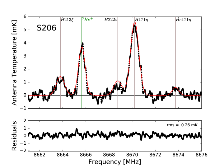
Figure 3: ${}^{3}{\rm He}^{+}$ spectrum of S206. Top Panel: The antenna temperature plotted as a function of rest frequency. The black dots are the observed GBT data. The solid red curve is the NEBULA model spectrum. It is not a Gaussian fit to the GBT data. The horizontal line is the zero level. The vertical lines mark the location of the ${}^{3}{\rm He}^{+}$ transition (green) and RRLs (gray). Bottom Panel: The residuals, model $-$ data, from the top panel. The rms of these residuals calculated across the entire sub-band is shown.

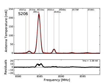
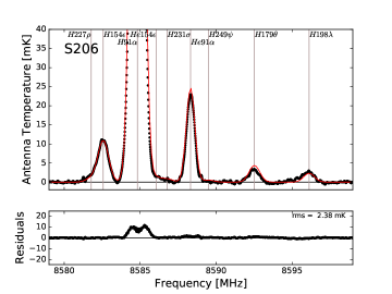
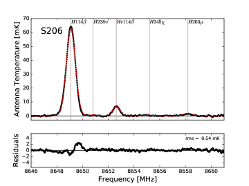
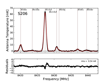
Figure 4: RRL spectra of S206 including the following sub-bands: H91$\alpha$ (top-left), expanded view of H91$\alpha$ (top-right), H114$\beta$ (bottom-left), and H115$\beta$ (bottom-right). See Figure 3 for details.

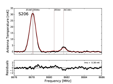
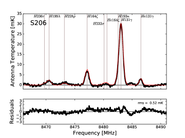
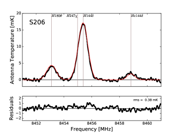
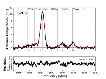
Figure 5: RRL spectra for S206 including the following sub-bands: H130$\gamma$ (top-left), H131$\gamma$ (top-right), H144$\delta$ (bottom-left), and H152$\epsilon$ (bottom-right). See Figure 3 for details.

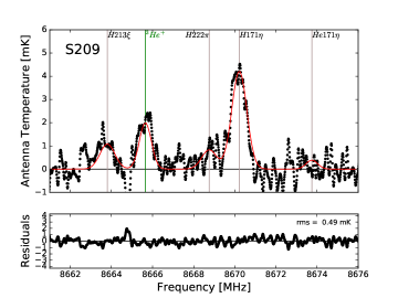
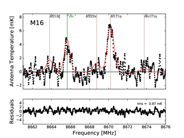
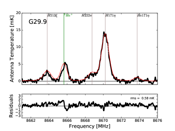
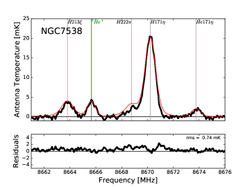
Figure 6: ${}^{3}{\rm He}^{+}$ spectrum of S209 (top-left), M16 (top-right), G29.9 (bottom-left), and NGC 7538 (bottom-right). See Figure 3 for details.

3.1 S206

S206 is a nearby, $D_{\rm sun}=3.3$$\,{\rm kpc}$, diffuse H ii region, but VLA continuum images do reveal some compact structures (Balser, 1995). The LTE NEBULA model matches the ${}^{3}{\rm He}^{+}$ spectrum very well with an ${\rm rms}=0.26$$\,{\rm mK}$, the lowest value in our sample (see Figure 3). There is no systematic trend in the RRL intensity with principal quantum number, n, indicating that non-LTE effects and pressure broadening are negligible (see Figures 4-5). The nebula is ionized by a single O4-O5 star and Fabry-Perot spectrophotometer data suggest that the H ii region should contain no neutral helium (Deharveng et al., 2000); therefore the ionization correction is $\kappa_{\rm i}=1.0$. We derive a ${}^{3}{\rm He}/{\rm H}$ abundance ratio of $1.89\pm\ 0.16\times 10^{-5}$ by number. This $1\,\sigma$ uncertainty implies an 8.5% accuracy in the abundance derivation.

3.2 S209

The large, diffuse H ii region S209 is the most distant in our sample with a Galactocentric radius of $R_{\rm gal}=16.2$$\,{\rm kpc}$. Spectrophotometry reveals an O9 and two B1 stars exciting S209 (Chini & Wink, 1984). The LTE NEBULA model contains several compact components (see Balser, 1995) and is a good fit to the data with a residual ${\rm rms}=0.49$$\,{\rm mK}$ in the ${}^{3}{\rm He}^{+}$ sub-band (Figure 6). Some instrumental baseline structure appears near the ${}^{3}{\rm He}^{+}$ transition, however, increasing the uncertainty of our measurement. This structure appears to exist in all scans and was not some intermittent feature (e.g., RFI). RRL data indicate that non-LTE effects are negligible (see Figures 10-11). A carbon line is visible in the brighter RRL transitions and arises from a primarily neutral photodissociation region (PDR) surrounding the ionized nebula (e.g., Wenger et al., 2013). Since the carbon emission line region is not part of the H ii region, and we only consider hydrogen and helium in our models, the NEBULA synthetic spectra do not include carbon lines. We determine a small ionization correction, $\kappa_{\rm i}=1.10$, and derive a ${}^{3}{\rm He}/{\rm H}$ abundance ratio of $1.10\pm\ 0.28\times 10^{-5}$ yielding a nominal uncertainty of 25%. The larger uncertainty is primarily due to a weak ${}^{3}{\rm He}^{+}$ line intensity (see Table 3).

3.3 M16

The Eagle nebula (M16) is a nearby, $D_{\rm sun}=2.0$$\,{\rm kpc}$, well-studied H ii region (White et al., 1999; Indebetouw et al., 2007). M16 is ionized by several O5-type stars (Hillenbrand et al., 1993). Using the VLA continuum data published in White et al. (1999), we model the Eagle nebula with several compact components and include a halo component from the 140 Foot continuum data. The NEBULA LTE model produces high-n RRLs that are a good fit to GBT spectra and therefore any non-LTE effects or pressure broadening should be negligible. Multiple velocity components are present in the GBT RRL spectra, however, with a weaker component at higher frequencies or lower velocities (see Figures 12-13). Nevertheless, the ${}^{3}{\rm He}^{+}$ sub-band residuals are well behaved with an ${\rm rms}=0.97$$\,{\rm mK}$. This is the largest ${}^{3}{\rm He}^{+}$ sub-band rms in our sample because of the short integration time on this source. A carbon RRL is also detected but as discussed above this transition arises from a PDR and not within the H ii region. Applying an ionization correction of $\kappa_{\rm i}=1.17$ yields a ${}^{3}{\rm He}/{\rm H}$ abundance ratio of $2.28\pm\ 0.48\times 10^{-5}$ and a nominal accuracy of 21%.

3.4 G29.9

The H ii region G29.9 is located near the large star formation complex associated with W43 at the end of the Galactic bar. There are few H ii regions within the extent of the bar (Bania et al., 2010), and moreover most H ii regions at these Galactic longitudes have uncertain distances. In our sample, G29.9 is the closest source to the Galactic Center with $R_{\rm gal}=4.4$$\,{\rm kpc}$. We did not obtain VLA continuum data for G29.9 in our previous work, so here we use a recent image from the GLOSTAR survey with the Jansky VLA (JVLA) at 5.8$\,{\rm GHz}$ (A. Brunthaler et al., in preparation). Figure 7 is the continuum image of G29.9 where the circle corresponds to the GBT HPBW.

We model G29.9 as two compact components based on the JVLA data and a halo component from the 140 Foot continuum (see Table 4). The LTE NEBULA model reveals non-LTE effects: the high-n RRL intensities are overpredicted by the model indicating pressure broadening. Figure 8 shows the RRL spectrum for the H115$\beta$ sub-band. The LTE NEBULA model (left panel) predicts brighter, narrower profiles. The non-LTE model including pressure broadening reduces these discrepancies, but the model RRL intensities for transitions with high n are still too large. We therefore apply a filling factor of 0.01 in the compact components to simulate higher local electron densities or additional density structure. The non-LTE models that include a clumpier medium are a better fit to the data as shown by the right panel in Figure 8. The feature to the right of the He115$\beta$ line corresponds to a blend between the C115$\beta$ and H215$\xi$ lines. Since we are not modeling carbon this feature is stronger than the NEBULA prediction. Simulations show that deriving the ${}^{3}{\rm He}/{\rm H}$ abundance ratio for sources with such structure have larger uncertainties (Balser et al., 1999a; Bania et al., 2007). To be conservative, we therefore use 3 times the rms of the residuals for the uncertainty in ${}^{3}{\rm He}^{+}/{\rm H^{+}}$.

The adopted NEBULA model for G29.9 is a reasonably good fit to the data with an ${\rm rms}=0.58$$\,{\rm mK}$ in the residuals of the ${}^{3}{\rm He}^{+}$ sub-band (Figure 6). There do appear to be multiple velocity components detected in the RRLs (see Figures 14-15). The low ${}^{4}{\rm He}^{+}/{\rm H^{+}}$ abundance ratio of 0.07 for G29.9 at $R_{\rm gal}=4.4$$\,{\rm kpc}$ produces a significant ionization correction of $\kappa_{\rm i}=1.39$. We derive a ${}^{3}{\rm He}/{\rm H}$ abundance ratio of $2.23\pm\ 0.76\times 10^{-5}$ yielding a nominal uncertainty of 34%.

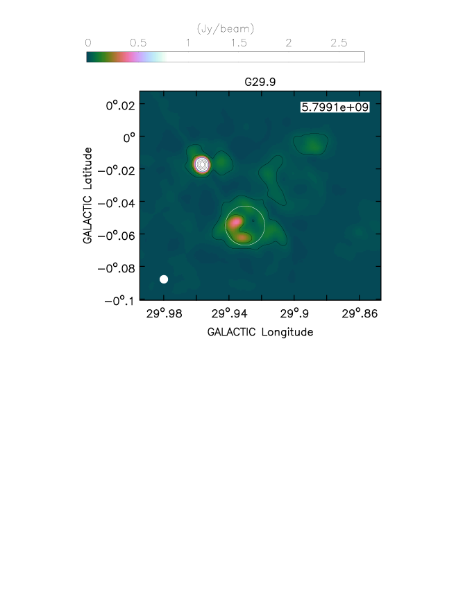
Figure 7: JVLA continuum image of G29.9 at 5.8$\,{\rm GHz}$. The contour levels are at 0.01, 0.05, 0.2, 0.4, 0.6, and 0.8 times the peak value of 2.76$\rm\,Jy\,beam^{-1}$. The rms noise in the image is 1$\rm\,mJy\,beam^{-1}$. The synthesized beam size is shown in the bottom-left corner. The white circle corresponds to the location and size of the GBT HPBW.

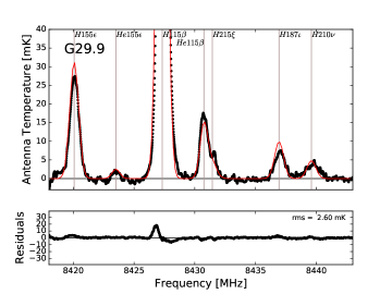
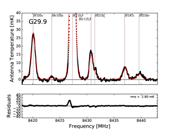
Figure 8: The H115$\beta$ sub-band for G29.9 assuming LTE (left) and including non-LTE effects (right). The C115$\beta$ line is visible to the right of the H115$\beta$ in the GBT data but carbon is not included in the models. See Figure 3 for details.

3.5 NGC 7538

NGC 7538 is a nearby, $D_{\rm sun}=2.8$, well-studied star formation region (e.g., Fallscheer et al., 2013; Luisi et al., 2016). The H ii region, also known as Sharpless 158 or S158, is a centrally diffuse source with a bright rim to the west. An O7 star located at the center of the nebula provides the ionizing photons (Deharveng et al., 1979). The VLA continuum data show several compact components with a very bright source to the south-east (Balser, 1995). The LTE NEBULA model does not provide a good fit to the GBT data. Similar to G29.9, non-LTE effects in the form of pressure broadening are present. Including pressure broadening and a filling factor of 0.15 for the compact components produces a reasonable fit to the data. To be conservative, we therefore use 3 times the rms of the residuals for the uncertainty in ${}^{3}{\rm He}^{+}/{\rm H^{+}}$.

The GBT baseline structure appears to be slightly worse for this source which explains some of the discrepancies between the model and data (see Figures 16-17). This is not unexpected since the total system temperature is higher for this brighter source and we have demonstrated that the baseline structure roughly scales with source intensity (see §2.4). For example, the continuum intensity for NGC 7538 is almost two times the next brightest source in our sample, G29.9. Nevertheless, the residuals in the ${}^{3}{\rm He}^{+}$ sub-band are reasonable with ${\rm rms}=0.74$$\,{\rm mK}$ (Figure 6). We derive an ionization correction of $\kappa_{\rm i}=1.06$ and a ${}^{3}{\rm He}/{\rm H}$ abundance ratio of $1.97\pm\ 1.08\times 10^{-5}$ giving a nominal uncertainty of 55%.

Based on the limited RRL data from the 140 Foot telescope, Bania et al. (2002) suggested that G29.9 and NGC 7538 were morphologically simple and therefore included them in their sample of sources with accurate ${}^{3}{\rm He}/{\rm H}$ determinations. The much richer RRL data set observed with the GBT show that these sources are not as simple as expected. Nevertheless, our NEBULA models match the data reasonably well and we include them in our analysis but with higher uncertainties.

4 The Time Evolution of the ${}^{3}{\rm He}$ Abundance

During the Big Bang era of primordial nucleosynthesis the light element ${}^{3}{\rm He}$ is predicted to be made in copious amounts with a final primordial ${}^{3}{\rm He}/{\rm H}$ abundance ratio of ${}^{3}{\rm He}/{\rm H}$ $\sim 10^{-5}$ by number (see Schramm & Wagoner, 1977; Boesgaard & Steigman, 1985; Cyburt, 2004, and references within). This primordial ${}^{3}{\rm He}$ abundance is further processed via stellar nucleosynthesis, but it is difficult to predict the net effect of the processes that produce and destroy ${}^{3}{\rm He}$ in stars. There is evidence that some stars do produce ${}^{3}{\rm He}$, however, since detection of ${}^{3}{\rm He}^{+}$ in a few PNe reveal abundances of ${}^{3}{\rm He}/{\rm H}$ $\sim 10^{-3}$, significantly higher than the primordial value (e.g., Balser et al., 2006).

Observations of ${}^{3}{\rm He}$ in Galactic H ii regions indicate a relatively flat ${}^{3}{\rm He}/{\rm H}$ radial abundance gradient across the Galactic disk, the ${}^{3}{\rm He}$ Plateau (Bania et al., 2002). Galactic chemical evolution models predict a higher rate of star formation in the central regions of the disk and we expect negative/positive radial gradients for elements that have a net production/destruction in stars (e.g., Chiappini et al., 1997; Schönrich & Binney, 2009; Lagarde et al., 2012; Minchev et al., 2014). The ${}^{3}{\rm He}$ Plateau, with zero radial gradient, was therefore interpreted as representing the primordial abundance with ${}^{3}{\rm He}/{\rm H}$ = $1.1\pm\ 0.2\times 10^{-5}$ (Bania et al., 2002). This value was independently confirmed with higher accuracy by combining results from the WMAP with BBN models (Romano et al., 2003).

The ${}^{3}{\rm He}$ Problem results from trying to reconcile the large ${}^{3}{\rm He}/{\rm H}$ abundance ratios found in a few PNe, consistent with standard stellar yields, with the essentially primordial values found in H ii regions (Galli et al., 1997). Rood et al. (1984) were the first to suggest that some sort of slow extra-mixing might be occurring to reduce the ${}^{3}{\rm He}$ abundance and that such mixing could also explain the depletion of ${}^{7}{\rm Li}$ in main-sequence stars and the low abundance ${}^{12}{\rm C}/^{13}{\rm C}$ ratios seen in low-mass RGB stars. Over the past 30 years the ${}^{3}{\rm He}$ Problem has galvanized a significant effort into improving stellar evolution models with more realistic mixing physics (e.g., Zahn, 1992; Charbonnel, 1995; Eggleton et al., 2006; Charbonnel & Zahn, 2007a). Lagarde et al. (2012) provide a potential solution to the ${}^{3}{\rm He}$ Problem by including the mixing effects of the thermohaline instability and rotation. Models that include this physics significantly reduce the present day ${}^{3}{\rm He}$ abundance. (They do not, however, deplete ${}^{3}{\rm He}$ below its primordial value.) Here we test these models by determining accurate ${}^{3}{\rm He}/{\rm H}$ abundance ratios in five H ii regions over a range of Galactocentric radii ($4.4\,{\rm kpc}<R_{\rm gal}<16.2\,{\rm kpc}$).

Figure 9 summarizes our results. Plotted is the present day ${}^{3}{\rm He}/{\rm H}$ abundance ratio as a function of $R_{\rm gal}$, corresponding to $\sim 10$$\,{\rm Gyr}$ of stellar and Galactic evolution that has occurred since the Milky Way formed. Our GBT H ii region results are shown as black circles. The magenta triangle corresponds to the ${}^{3}{\rm He}$ abundance in the local interstellar medium (LISM) from in situ measurements on the spacecraft Ulysses (Gloeckler & Geiss, 1996). The primordial ${}^{3}{\rm He}$ abundance, represented by the gray horizontal region, is based on BBN and WMAP results and their uncertainties (Cyburt et al., 2008, also see Cyburt et al. (2016); Coc & Vangioni (2017)). The models of Lagarde et al. (2012) are shown as three different curves. The top (solid red) curve corresponds to standard ${}^{3}{\rm He}$ stellar yields and is inconsistent with the present day H ii region ${}^{3}{\rm He}$ abundances. The two lower curves (dashed green and dotted cyan) include the thermohaline instability and rotation-induced mixing. They are slightly higher than the data but consistent with the notion that there is a small net production of ${}^{3}{\rm He}$ in stars. The models do not predict a linear relationship between ${}^{3}{\rm He}/{\rm H}$ and $R_{\rm gal}$, but for reference we show a linear fit to the data which has a slope of $-0.116\pm\ 0.022\,\times\,$$10^{-5}$ kpc^-1.

Clearly more accurate ${}^{3}{\rm He}/{\rm H}$ abundances are needed for H ii regions located at smaller $R_{\rm gal}$ where the models predict an upturn in the ${}^{3}{\rm He}$ abundance. The G29.9 ${}^{3}{\rm He}/{\rm H}$ abundance derivation may suffer from additional, unknown systematic error. Previously the sample of morphologically simple H ii regions at $R_{\rm Gal}\lesssim\ 4$$\,{\rm kpc}$ was extremely small due in part to the Galactic distribution of the H ii region population. New H ii region discovery surveys, however, have the potential to provide new targets in this critical $R_{\rm gal}$ zone (Bania et al., 2010, 2012; Anderson et al., 2011, 2015, 2018; Brown et al., 2017). Finally, a new generation of GCE models would improve our understanding of the Galactic chemical evolution of ${}^{3}{\rm He}$. It may be that beside the stellar ${}^{3}{\rm He}$ yields other assumptions made in the current GCE models are important.

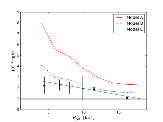
Figure 9: Evolution of ${}^{3}{\rm He}$ within the Milky Way disk. Plotted is the ${}^{3}{\rm He}/{\rm H}$ abundance ratio as a function of Galactocentric radius. The GBT results derived here for H ii regions are shown as black circles. The magenta triangle is the LISM abundance derived by Gloeckler & Geiss (1996) from their Ulysses measurement. The curves correspond to three models from Lagarde et al. (2012). These models predict the ${}^{3}{\rm He}/{\rm H}$ abundance ratio after 10$\,{\rm Gyr}$ of stellar processing has modified the primordial abundance produced during BBN. They are not fits to the H ii region ³He/H abundances derived from observations shown here. Model A (solid red) uses standard yields for all stars; model B (blue dashed) considers thermohaline instability and rotation-induced mixing for 96% of low-mass stars ($M\leq\ 2.5$$\,M_{\odot}$) and 100% of high-mass stars ($M>2.5$$\,M_{\odot}$); and model C (cyan dotted) considers thermohaline instability and rotation-induced mixing for all stars. The gray horizontal region is the primordial abundance range of ${}^{3}{\rm He}/{\rm H}$ = $1.00\pm\ 0.07\times 10^{-5}$ from WMAP and BBN (Cyburt et al., 2008). The green solid line is a linear fit to the data (H ii regions and LISM) using orthogonal distance regression which finds a slope of $-0.116\pm\ 0.022\,\times\,$$10^{-5}$ kpc^-1.

Charbonnel & Zahn (2007b) proposed that strong magnetic fields in RGB stars that evolved from Ap stars could inhibit mixing from the thermohaline instability and thereby explain the few PNe with high values of ${}^{3}{\rm He}/{\rm H}$. Lagarde et al. (2012) simulates the effects of such stars on the evolution of ${}^{3}{\rm He}$ (Model B), but the results are only slightly different than if thermohaline mixing was occurring in all stars (Model C). We cannot distinguish between these models with our H ii region data. A high ${}^{3}{\rm He}/{\rm H}$ abundance ratio derived for even a single PN would indicate that some mechanism must be at play to inhibit the extra mixing in this object. Extra-mixing should otherwise occur in all low-mass stars. There are three PNe with published ${}^{3}{\rm He}^{+}$ detections: NGC 3242 (Rood et al., 1992; Balser et al., 1997, 1999b), J320 (Balser et al., 2006), and IC 418 (Guzman-Ramirez et al., 2016). The ${}^{3}{\rm He}/{\rm H}$ abundance ratio derived for these detections range from $2\times 10^{-4}$ to $6\times 10^{-3}$, an order of magnitude higher than the abundances found in H ii regions.

Observations of the ${}^{3}{\rm He}^{+}$ spectral transition are challenging. Accurate measurement of these weak, broad lines requires significant integration time and a stable, well-behaved spectrometer (Balser et al., 1994). This is particularly true when observing ${}^{3}{\rm He}^{+}$ in PNe since the lines are weaker and broader than for H ii regions. Much effort went into detecting ${}^{3}{\rm He}^{+}$ in NGC 3242 using the Max-Planck Institut für Radioastronomie (MPIfR) 100$\,{\rm m}$ and the NRAO 140 Foot telescopes. Nevertheless, preliminary GBT observations of ${}^{3}{\rm He}^{+}$ in NGC 3242 do not confirm the MPIfR 100$\,{\rm m}$ result (Bania et al., 2010). One sign that there were problems with the NGC 3242 data was the large discrepancy between the model and observed intensity of the H171$\eta$ RRL (See Figure 3 in Balser et al., 1999b). Additional GBT observations toward NGC 3242 have been taken and we plan to perform detailed modeling of this PNe.

Guzman-Ramirez et al. (2016) report a ${}^{3}{\rm He}^{+}$ detection in IC 418 with a SNR of 5.7 using the National Aeronautics and Space Administration (NASA) Deep Space Station 63 (DSS-63). They have simultaneously observed many RRLs but do not provide any detailed models to assess their accuracy. For example, the ${}^{4}{\rm He}/{\rm H}$ abundance ratio is 0.11 and 0.037 for the 91$\alpha$ and 92$\alpha$ RRLs, respectively. These adjacent RRLs should produce the same result yet they are a factor of 3 different. We are therefore very suspicious of the claimed detection of ${}^{3}{\rm He}^{+}$ in IC 418.

The advantage of interferometers like the VLA is that much, but not all, of the instrumental baseline structure is correlated out. We therefore deem that the detection in J320 with the VLA is more robust. The SNR is only 4, but when averaging over a halo region the SNR increases to 9. Nevertheless, the limited bandwidth of the VLA did not allow the simultaneous observation of many RRLs to constrain the models and assess the spectral baseline stability. Observations with the much improved Jansky VLA would provide for a more robust evaluation.

5 Summary

Studies of ${}^{3}{\rm He}$ provide important constraints to Big Bang nucleosynthesis, stellar evolution, and Galactic evolution. Standard stellar evolution models that predict the production of copious amounts of ${}^{3}{\rm He}$ in low-mass stars, consistent with the high ${}^{3}{\rm He}/{\rm H}$ abundance ratios found in a few planetary nebulae, are at odds with the approximately primordial values determined for Galactic H ii regions. This inconsistency is called the ${}^{3}{\rm He}$ Problem. Models that include mixing from the thermohaline instability and rotation provide a mechanism to reduce the enhanced ${}^{3}{\rm He}/{\rm H}$ abundances during the RGB stage (Charbonnel & Lagarde, 2010; Lagarde et al., 2011). These yields together with GCE models predict modest ${}^{3}{\rm He}$ production by stars over the lifetime of the Milky Way (Lagarde et al., 2012). The scatter of the ${}^{3}{\rm He}$ Plateau abundances determined by Bania et al. (2002) is large and spans the range of abundances predicted by Lagarde et al. (2012).

Here we detect ${}^{3}{\rm He}^{+}$ emission in five morphologically simple Galactic H ii regions with the GBT over a wide range of Galactocentric radii: $4.4\,{\rm kpc}<R_{\rm gal}<16.2\,{\rm kpc}$. Our goal is to derive accurate abundance ratios for a small sample of sources to uncover any trend in the ${}^{3}{\rm He}/{\rm H}$ abundance with $R_{\rm gal}$, and to compare our results with the predictions of Lagarde et al. (2012). We use the radiative transfer program NEBULA, together with GBT measurements of over 35 RRL transitions, to constrain H ii region models and determine accurate ${}^{3}{\rm He}/{\rm H}$ abundance ratios. The RRLs are measured with high SNRs and allow us to assess the quality of the spectral baselines which is critical to measuring wide, weak lines accurately. We find that S209, S209, and M16 are indeed simple sources that are well characterized by LTE models. G29.9 and NGC 7538, however, contain density structure on spatial scales not probed by our VLA observations and also require non-LTE models; the ${}^{3}{\rm He}/{\rm H}$ abundance ratios derived for these sources are therefore less accurate. We apply an ionization correction to convert ${}^{3}{\rm He}^{+}/{\rm H^{+}}$ to ${}^{3}{\rm He}/{\rm H}$ using ${}^{4}{\rm He}$ RRLs since there may exist some neutral helium within the H ii region.

We determine a ${}^{3}{\rm He}/{\rm H}$ radial gradient of $-0.116\pm\ 0.022\,\times\,$$10^{-5}$ kpc^-1, consistent with the overall trend predicted by Lagarde et al. (2012). Our ${}^{3}{\rm He}/{\rm H}$ abundance ratios, however, are typically slightly less than the models that include thermohaline mixing. We do not have enough accuracy to determine whether or not strong magnetic fields in some stars could inhibit the thermohaline instability as predicted by (Charbonnel & Zahn, 2007b). More conclusive measurements of ${}^{3}{\rm He}^{+}$ in PNe would be useful to confirm that indeed some stars do produce significant amounts of ${}^{3}{\rm He}$.

Appendix A Galactic H ii Region Radio Recombination Line Spectra

For completeness we include RRL spectra for S209 (Figures 10-11), M16 (Figures 12-13), G29.9 (Figures 14-15), and NGC 7538 (Figures 16-17). Plotted in the top panel of each figure is the antenna temperature as a function of rest frequency. The black points display the observed spectrum and the red curve is the NEBULA model. The vertical lines mark the location of various RRL transitions. The residuals of the model and data are shown in the bottom panel of each figure.

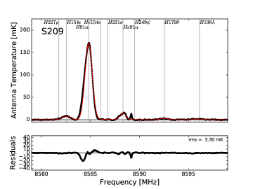
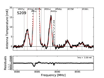
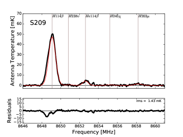
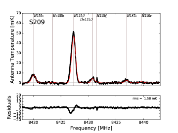
Figure 10: RRL spectra of S209 including the following sub-bands: H91$\alpha$ (top-left), expanded view of H91$\alpha$ (top-right), H114$\beta$ (bottom-left), and H115$\beta$ (bottom-right). See Figure 4 for details.

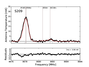
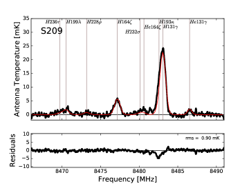
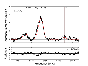
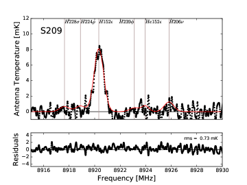
Figure 11: RRL spectra for S209 including the following sub-bands: H130$\gamma$ (top-left), H131$\gamma$ (top-right), H144$\delta$ (bottom-left), and H152$\epsilon$ (bottom-right). See Figure 5 for details.

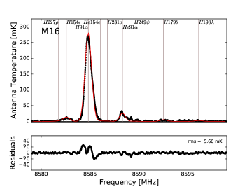
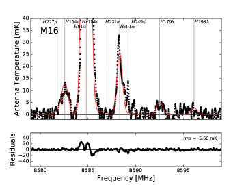
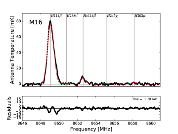
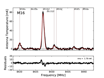
Figure 12: RRL spectra of M16 including the following sub-bands: H91$\alpha$ (top-left), expanded view of H91$\alpha$ (top-right), H114$\beta$ (bottom-left), and H115$\beta$ (bottom-right). See Figure 4 for details.

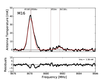
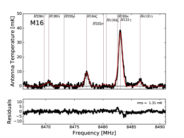
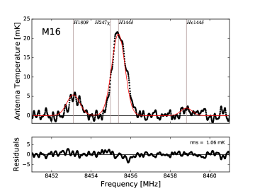
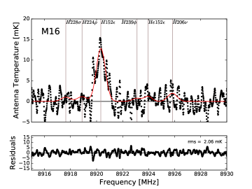
Figure 13: RRL spectra for M16 including the following sub-bands: H130$\gamma$ (top-left), H131$\gamma$ (top-right), H144$\delta$ (bottom-left), and H152$\epsilon$ (bottom-right). See Figure 5 for details.

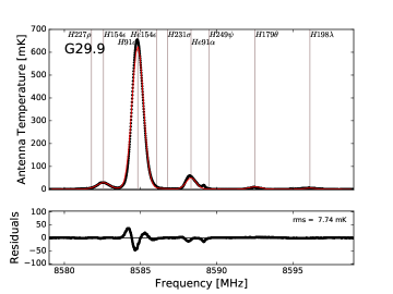
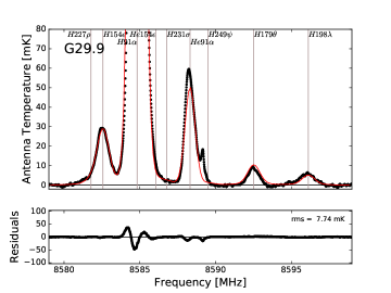
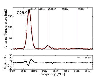
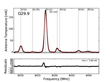
Figure 14: RRL spectra of G29.9 including the following sub-bands: H91$\alpha$ (top-left), expanded view of H91$\alpha$ (top-right), H114$\beta$ (bottom-left), and H115$\beta$ (bottom-right). See Figure 4 for details.

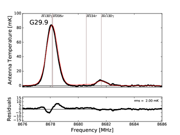
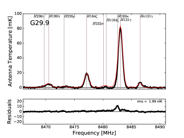
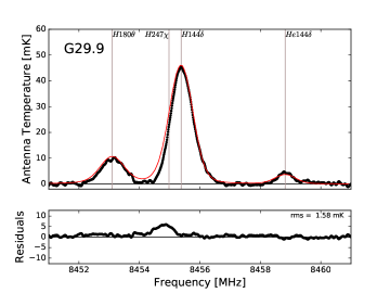
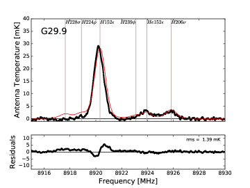
Figure 15: RRL spectra for G29.9 including the following sub-bands: H130$\gamma$ (top-left), H131$\gamma$ (top-right), H144$\delta$ (bottom-left), and H152$\epsilon$ (bottom-right). See Figure 5 for details.

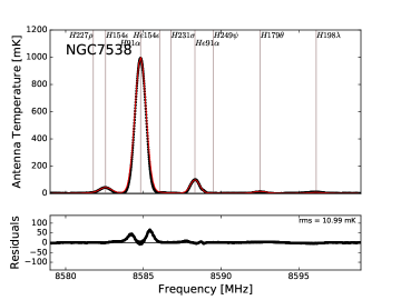
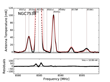
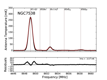
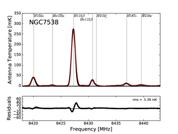
Figure 16: RRL spectra of NGC7538 including the following sub-bands: H91$\alpha$ (top-left), expanded view of H91$\alpha$ (top-right), H114$\beta$ (bottom-left), and H115$\beta$ (bottom-right). See Figure 4 for details.

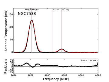
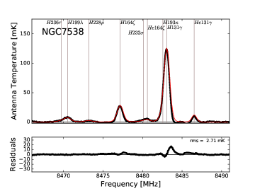
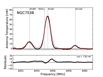
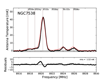
Figure 17: RRL spectra for NGC7538 including the following sub-bands: H130$\gamma$ (top-left), H131$\gamma$ (top-right), H144$\delta$ (bottom-left), and H152$\epsilon$ (bottom-right). See Figure 5 for details.

References

- Anderson et al. (2011) Anderson, L. D., Bania, T. M., Balser, D. S., & Rood, R. T. 2011, ApJS, 194, 32
- Anderson et al. (2015) Anderson, L. D., Armentrout, W. P., Johnstone, B. M., et al. 2015, ApJS, 221, 26
- Anderson et al. (2018) Anderson, L. D., Armentrout, W. P., Luisi, M., et al. 2018, ApJS, 234, 33
- Balser (1995) Balser, D. S. 1995, Ph.D. thesis, Boston Univ.
- Balser (2006) Balser, D. S. 2006, AJ, 132, 2326
- Balser & Bania (2018) Balser, D. S., & Bania, T. M. 2018, NEBULA: Radiative transfer code of ionized nebulae at radio wavelengths, Astrophysics Source Code Library, ascl:1809.009
- Balser et al. (1995) Balser, D. S., Bania, T. M., Rood, R. T., & Wilson, T. L. 1995, ApJS, 100, 371
- Balser et al. (1997) Balser, D. S., Bania, T. M., Rood, R. T., & Wilson, T. L. 1997, ApJ, 483, 320
- Balser et al. (1999a) Balser, D. S., Bania, T. M., Rood, R. T., & Wilson, T. L. 1999a, ApJ, 510, 759
- Balser et al. (1999b) Balser, D. S., Rood, R. T., & Bania, T. M. 1999b, ApJ, 522, L73
- Balser et al. (1994) Balser, D. S., Bania, T. M., Brockway, C. J., Rood, R. T., & Wilson, T. L. 1994, ApJ, 430, 667
- Balser et al. (2006) Balser, D. S., Goss, W. M., Bania, T. M., & Rood, R. T. 2006, ApJ, 640, 360
- Bania et al. (2012) Bania, T. M., Anderson, L. D., & Balser, D. S. 2012, ApJ, 759, 96
- Bania et al. (2010) Bania, T. M., Anderson, L. D., Balser, D. S., & Rood, R. T. 2010, ApJ, 718, L106
- Bania et al. (2007) Bania, T. M., Balser, D. S., Rood, R. T., & Wilson, T. L., & LaRacque, J. M. 2007, ApJ, 664, 915
- Bania et al. (2002) Bania, T. M., Rood, R. T., & Balser, D. S. 2002, Natur, 415, 54
- Bania et al. (1987) Bania, T. M., Rood, R. T., & Wilson, T. L. 1987, ApJ, 323, 30
- Bania et al. (2016) Bania, T., Wenger, T., Balser, D., & Anderson, L. 2016, TMBIDL: Single Dish Radio Astronomy Data Reduction Package, Astrophysics Source Code Library, ascl:1605.005
- Boesgaard & Steigman (1985) Boesgaard, A. M. & Steigman, G. T. 1985, ARA&A, 23, 319
- Boothroyd & Sackmann (1999) Boothroyd, A. I., & Sackmann, I.-J. 1999, ApJ, 510, 232
- Brown et al. (2017) Brown, C., Jordan, C., Dickey, J. M., et al. 2017, AJ, 154, 23
- Carigi & Peimbert (2008) Carigi, L., & Peimbert, M. 2008, RMxAA, 44, 341
- Charbonnel (1995) Charbonnel, C. 1995, ApJ, 453, L41
- Charbonnel et al. (1998) Charbonnel, C., Brown, J. A., & Wallerstein, G. 1998, A&A, 332, 204
- Charbonnel & Do Nascimento (1998) Charbonnel, C., & Do Nascimento, J. D., Jr. 1998, A&A, 336, 915
- Charbonnel & Lagarde (2010) Charbonnel, C., & Lagarde, N. 2010, A&A, 522, A10
- Charbonnel & Zahn (2007a) Charbonnel, C., & Zahn, J.-P. 2007a, A&A, 467, L15
- Charbonnel & Zahn (2007b) Charbonnel, C., & Zahn, J.-P. 2007b, A&A, 467, L29
- Chiappini et al. (1997) Chiappini, C., Matteucci, F., & Gratton, R. 1997, ApJ, 477, 765
- Chiappini et al. (2002) Chiappini, C., Renda, A., & Matteucci, F. 2002, A&A, 395, 789
- Chini & Wink (1984) Chini, R., & Wink, J. E. 1984, A&A, 139, L5
- Coc & Vangioni (2017) Coc, A., & Vangioni, E. 2017, IJMPE , 26, 1741002
- Cyburt (2004) Cyburt, R. H. 2004, Phys. Rev. D, 70, 023505
- Cyburt et al. (2008) Cyburt, R. H., Fields, B. D., & Olive, K. A. 2008, JCAP, 11, 12
- Cyburt et al. (2016) Cyburt, R. H., Fields, B. D., Olive, K. A., & Yeh, T.-H. 2016, RvMP, 88, 015004
- Dearborn et al. (1996) Dearborn, D. S. P., Steigman, G., & Tosi, M. 1996, ApJ, 465, 887
- Deharveng et al. (2000) Deharveng, L., Pea, M., Caplan, J., & Costero, R. 2000, MNRAS, 311, 329
- Deharveng et al. (1979) Deharveng, L., Lortet, M. C., & Testor, G. 1979, A&A, 71, 151
- Denissenkov (2010) Denissenkov, P. A. 2010, ApJ, 723, 563
- Denissenkov & Merryfield (2011) Denissenkov, P. A. & Merryfield, W. J. 2011, ApJ, 727, L8
- Eggleton et al. (2006) Eggleton, P. P., Dearborn, D. S. P., & Lattanzio, J. C. 2006, Sci, 314, 1580
- Fallscheer et al. (2013) Fallscheer, C, Reid, M. A., Di Francesco, J. et al. 2013, ApJ, 773, 102
- Fisher et al. (2003) Fisher, J. R., Norrod, R. D., & Balser, D. S. 2003, NRAO Electronics Division Internal Report, No. 312
- Forestini & Charbonnel (1997) Forestini, M., & Charbonnel, C. 1997, A&AS, 123, 241
- Galli et al. (1995) Galli, D., Palla, F., Ferrini, F., & Penco, U. 1995, ApJ, 443, 536
- Galli et al. (1997) Galli, D., Stanghellini, L., Tosi, M., & Palla, F., ApJ, 477, 218
- Geiss & Gloeckler (1998) Geiss, J., & Gloeckler, G. 1998, SSRv, 84, 239
- Ghigo et al. (2001) Ghigo, F., Maddalena, R., Balser, D., & Langston, G. 2001, GBT Commissioning Memo 10
- Gloeckler & Geiss (1996) Gloeckler, G., & Geiss, J. 1996, Natur, 381, 210
- Gordon (1976) Gordon, M. A., 1976, in Methods of Experimental Physics. Vol. 12. Astrophysics. Part C: Radio observations, 277