Valley engineering by strain in Kekulé-distorted graphene

Abstract

A Kekulé bond texture in graphene modifies the electronic band structure by folding the Brillouin zone and bringing the two inequivalent Dirac points to the center. This can result, in the opening of a gap (Kek-O) or the locking of the valley degree of freedom with the direction of motion (Kek-Y). We analyze the effects of uniaxial strain on the band structure of Kekulé-distorted graphene for both textures. Using a tight-binding approach, we introduce strain by considering the hopping renormalization and corresponding geometrical modifications of the Brillouin zone. We numerically evaluate the dispersion relation and present analytical expressions for the low-energy limit. Our results indicate the emergence of a Zeeman-like term due to the coupling of the pseudospin with the pseudomagnetic strain potential which separates the valleys by moving them in opposite directions away from the center of the Brillouin zone. For the Kek-O phase, this results in a competition between the Kekulé parameter that opens a gap and the magnitude of strain which closes it. While for the Kek-Y phase, in a superposition of two shifted Dirac cones. As the Dirac cones are much closer in the supperlattice reciprocal space that in pristine graphene, we propose strain as a control parameter for intervalley scattering.

I Introduction

In graphene, the electronic properties are dominated by the two inequivalent local minima in the conduction band, located at the high symmetry Brillouin zone points $\bm{K_{+}}$ and $\bm{K_{-}}$, and referred to the $K_{D}^{+}$ and $K_{D}^{-}$ valley, respectively. This endows low-energy electrons with an additional degree of freedomSchaibley , known as valley isospin. In pristine membranesneto2009electronic , these two valleys have gapless Dirac spectra, which are degenerate in energy, related by time-reversal symmetry, and well separated in reciprocal space by the Kekulé vector $\bm{G}=\bm{K_{+}}-\bm{K_{-}}$. However, if graphene is subject to a periodic perturbation, with a spatial periodicity associated with $\bm{G}$ (Kekulé distorsion), a superlattice with a tripled unit cell (of the size of a hexagonal ring) is formed. As a consequence, the two Dirac cones at opposite corners ($K_{D}^{+}$ and $K_{D}^{-}$) are folded onto the center $\Gamma$ of the new hexagonal superlattice Brillouin zoneChamon2007 . Almost twenty years ago, Claudio Chamon showed that a bond distortion mimicking the Kekulé structure for benzene (Kek-O) provides such a periodicity in graphene, which opens a gap by mixing the two valley speciesChamon2000 . Interestingly, graphene with a Kek-O distortion is also expected to show topological charge fractionalizationChamon2007 , and other topological propertieswakabayashi ; wu2016 .

Although experimentally achievable in analogues of graphenemanoharan ; li-phonons , up to now the Kek-O phase in graphene has not become a physical reality. Nevertheless, theoretical studies suggest that the Kek-O phase can be obtained by depositing graphene on top of a topological insulatorontop , by applying uniaxial strainSorella or by placing atoms adsorbed on its surfacecheianov . The latter proposal was pursued by Gutierrez et al.Gutierrez , who experimentally found another Kekulé distorsion, the Kekulé-Y (Kek-Y) phase, which consists of a periodic modification of the three bonds (in form of the letter Y) surrounding one of the atoms of the new hexagonal unit cell. Recently, Gamayun et al showed that this Kek-Y bond texture results in the locking of valley isospin with the direction of motion (momentum), breaking the valley degeneracy while preserving the massless character of the Dirac fermions. This effect opens a new way to control the valley degree of freedom in grapheneGamayun .

There have been several theoretical proposals to manipulate the valley degree of freedom in graphenerycerz2007valley ; Fujita2010 ; guinea2013 ; wang2014 ; grujic2014 ; ren2015 ; carrillo2016strained ; stegmann2016valley ; jones2017quantized ; wu2016full ; Cazalilla ; Asmar-minimal ; Luo2017 ; Beenakker ; Yee2017 ; Brown2018 ; settnes2017valley ; milovanovic2016strained ; Roche ; carrillo2018enhanced ; stegmann2018 ; zhai2018local ; ValleyPRL2018 , including the celebrated Valley Hall effectXiao2007 produced by Berry curvaturexiao-review , and the use of strainAMORIM20161 ; NaumisReview ; vozmediano2010gauge . The former has been recently observed in graphene superlattices by nonlocal transport measurementgorbachev2014 ; komatsu2018 . The effects of the latterCrommie ; Theory-LL01 ; Theory-LL02 are strong, measurable and expected to be valley asymmetricsettnes2017valley ; milovanovic2016strained ; Roche ; carrillo2018enhanced . In fact, both couple asymmetrically with each valley by breaking the inversion symmetry while preserving time reversal. Nevertheless, strain offers the advantage of being tunable and it is in intimate relation with the kekulé phase, since this phase is expected to appear in the presence of uniaxial strainSorella ; guinea . In general, uniaxial strain alters the band structure of graphene by (1) distorting the shape of the Brillouin zone, thus changing the geometrical position of the high symmetry points due to the modification of the lattice vectorsoliva-Leyva-PRB , and (2) moving the Dirac cones away from the high symmetry points, since it changes unevenly the three hopping energies connecting neighboring sitesPereira2009 . These two effects should be taken into account to obtain the low energy approximation for graphene, otherwise unphysical results are obtained even in the simplest casesoliva-Leyva-PRB ; oliva-leyva-physA .

Inspired by the results described above, in the present manuscript we evaluate the effect of uniaxial strain on Kekulé distorted graphene in both phases: Kek-O and Kek-Y. Using the tight binding approximation, we write the Hamiltonian for Kekulé-distorted graphene and introduce strain by changing the hopping integrals and atomic positions in the lattice. The layout of this paper is the following: In Section II, we present the model, as well as the resulting band structures. Section III is devoted to obtaining a low-energy effective Hamiltonian; and in Section IV, we provide the final conclusions and remarks.

II Hamiltonian for strained Kekulé distorted graphene

Let us start by considering a pure Kekulé pattern on unstrained graphene. The electronic properties are well described by a tight-binding Hamiltonian for a single $\pi$-orbital per carbon site Gamayun ,

$$H=-\sum_{\bm{r}}\sum_{j=1}^{3}t_{\bm{r},j}a_{\bm{r}}^{\dagger}b_{\bm{r}+\bm{\delta}_{j}}+H.c.,$$ (1)

where $\bm{r}$ runs over the atomic positions of graphene’s sublattice A, given by $\bm{r}=n_{1}\bm{a}_{1}+n_{2}\bm{a}_{2}$, with $n_{1}$ and $n_{2}$ integers. The lattice vectors are $\bm{a}_{1}=a(-\frac{\sqrt{3}}{2},\frac{3}{2})$, and $\bm{a}_{2}=a(\frac{\sqrt{3}}{2},\frac{3}{2})$, with $a=1.42$ Å. Each vector $\bm{\delta}_{i}$ points to one of the three nearest-neighbor sites belonging to sublattice B, and surrounding the site located at a given $\bm{r}$, as shown in Fig. 1 $[\bm{\delta}_{1}=a(\frac{\sqrt[]{3}}{2},-\frac{1}{2})$, $\bm{\delta}_{2}=-a(\frac{\sqrt[]{3}}{2},\frac{1}{2})$, and $\bm{\delta}_{3}=a(0,1)]$. The set of tight-binding parameters describing the bond-density wave of the Kekulé pattern is given byGamayun

$$\begin{split}t_{\bm{r},j}=t_{0}\Big{[}&1+\Delta e^{i(p\bm{K}_{+}+q\bm{K}_{-})\cdot\bm{\delta}_{j}+i\bm{G}\cdot\bm{r}}\\ &+\Delta^{*}e^{-i(p\bm{K}_{+}+q\bm{K}_{-})\cdot\bm{\delta}_{j}-i\bm{G}\cdot\bm{r}}\Big{]},\end{split}$$ (2)

where $t_{0}\approx 2.7eV$ is the hopping-parameter for pristine graphene, $\Delta=e^{i2\pi m/3}\Delta_{0}$ is the Kekulé coupling with amplitude $\Delta_{0}$ and $m$ an arbitrary integer number, $\bm{K}_{\pm}=\frac{2\pi}{9a}\sqrt{3}(\pm 1,\sqrt{3})$ are the high-symmetry points of graphene such that the Kekulé wave vector is $\bm{G}=\frac{4\pi}{9a}\sqrt{3}(1,0)$. Given that $p$ and $q$ are integers, the value of the Kekulé-distorted hopping-parameter $t_{\bm{r},j}$ oscillates in space between the values $t_{0}(1-\Delta_{0})$ and $t_{0}(1+2\Delta_{0})$, generating a Kekulé texture accordingly to the index Gamayun

$$\nu=1+q-p\mod 3,$$ (3)

with a Kek-O texture for $\nu=0$, and Kek-Y for $\nu=\pm 1$.

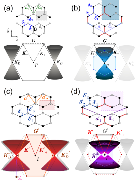
Figure 1: Lattices and Brillouin Zones for: (a) pristine graphene, (b) Kek-Y distorted graphene (red bonds), (c) strained graphene, and (d) Kek-Y distorted graphene with strain. The Kekulé and strained Kekulé vectors $\bm{G}$ and $\bm{G}^{\prime}$ are indicated in the upper side of the hexagonal Brillouin zones for each case. In a), the Dirac cones for pristine graphene are indicated in dark gray. In b), the gray Dirac cones are folded into a degenerate Dirac cone (in blue) to the $\Gamma$ point, while in c), the original Dirac cones (in gray) are deformed and translated to the points $\bm{K}_{D}^{\pm}$, as indicated in red. In d), the Dirac cones (gray) are folded into the $\Gamma$ point, but the strain breaks the degeneracy resulting in the overlapping of two shifted Dirac cones, both indicated in purple.

Let us now consider the effects of strain. When a strain field $\bm{u}=(u_{x}(x,y),u_{y}(x,y))$ is applied to pristine graphene, the atomic positions $\bm{r}$ change to,

$$\bm{r}^{\prime}=(1+\bar{\epsilon})\cdot\bm{r},$$ (4)

where $\bar{\epsilon}$ is the strain tensor with components NaumisReview ,

$$\epsilon_{ij}=\frac{1}{2}\left(\frac{\partial u_{j}}{\partial x_{i}}+\frac{\partial u_{i}}{\partial x_{j}}\right).$$ (5)

where $i=x,y$ and $j=x,y$. The local distance between neighbor atoms gets modified accordingly NaumisReview ,

$$\bm{\delta}_{j}^{\prime}=(1+\bar{\epsilon})\cdot\bm{\delta}j,$$ (6)

and similarly the basis vectors.

$$\bm{a}_{j}^{\prime}=(1+\bar{\epsilon})\cdot\bm{a}_{j},$$ (7)

as seen in Fig. 1.

Notice that the considered strain is uniform and thus space independent. This case also serves as a first approximation for smooth strain profiles. As the strain is uniform, it can be written as follows,

$$\bar{\epsilon}=\left[{\begin{array}[]{cc}\epsilon_{xx}&\epsilon_{xy}\\ \epsilon_{xy}&\epsilon_{yy}\\ \end{array}}\right]=\left[{\begin{array}[]{cc}\epsilon_{Z}&\epsilon_{S}\\ \epsilon_{S}&\epsilon_{A}\\ \end{array}}\right].$$ (8)

In the previous expression, the space-independent parameters ${{\epsilon}_{A}}$ and ${{\epsilon}_{Z}}$ denote uniaxial strain applied along the zigzag and armchair directions, respectively, and $\epsilon_{S}$ is the shear strain. This tensor can be parametrized in terms of $\epsilon$ (the magnitude of the applied strain), its angular direction $\theta$ (with respect to the $x$-axis), and $\rho$, the Poisson ratio which relates the strain components with a value of $\rho=0.165$ for grapheneBotello2018 ,

$$\bar{\epsilon}=\left[{\begin{array}[]{cc}\epsilon(\cos^{2}\theta-\rho\sin^{2}\theta)&\epsilon(1+\rho)\cos\theta\sin\theta\\ \epsilon(1+\rho)\cos\theta\sin\theta&\epsilon(\sin^{2}\theta-\rho\cos^{2}\theta)\\ \end{array}}\right].$$ (9)

In the absence of a Kekulé pattern, the tight-binding parameter for the strained lattice is given by NaumisReview

$$t_{j}=t_{0}e^{-\beta\left(\frac{|\bm{\delta}_{j}^{\prime}|}{a}-1\right)},$$ (10)

where $\beta$ is the Gruneissen parameter, estimated to be $\beta\approx 3$ for graphene. It is important to remark that second- and third-neighbor interactions are always present, which depend upon the bond torsion-angle Botello2018 . These effects will be neglected here as a first approximation.

Now, we can combine strain with a Kekulé pattern as follows: First, due to the modified distance between sites, the tight-binding parameter $t_{0}$ in Eq. 2 is replaced by $t_{j}$, defined by Eq. 10. Second, we need to keep the Kekulé density-wave bond ordering. Thus, we can proceed by observing that the phases of the pattern are preserved ifGamayun ,

$$(p\bm{K}_{+}+q\bm{K}_{-})\cdot\bm{\delta}_{j}+\bm{G}\cdot\bm{r}=(p\bm{K}_{+}^{\prime}+q\bm{K}_{-}^{\prime})\cdot\delta_{j}^{\prime}+\bm{G}^{\prime}\cdot\bm{r}^{\prime},$$ (11)

as long as we define,

$$\bm{K}_{\pm}^{\prime}=(1+\bar{\epsilon})^{-1}\cdot\bm{K}_{\pm},$$ (12a)

$$\bm{G}^{\prime}=\bm{K}_{+}^{\prime}-\bm{K}_{-}^{\prime}=(1+\bar{\epsilon})^{-1}\cdot\bm{G}.$$ (12b)

this constitutes a systematical procedure to introduce uniaxial strain to graphene supperlattices.

Although it is tempting to think of $\bm{K}_{\pm}^{\prime}$ as the reciprocal transformation of Eq. 4 for the high-symmetry points of the deformed lattice, in general, it turns out that the transformed reciprocal vectors of the high symmetry points of pristine graphene do not coincide with the high-symmetry points of the deformed lattice Brillouin zonePereira2009 ; NaumisReview . Moreover, strain changes the symmetry of the Bravais lattice. The high-symmetry points of the first Brillouin zone strained lattice must be labeled differently. As an example, the $\bm{K}_{\pm}$ points of the P6/mmm space group after a uniaxial strain are replaced by the $\bm{F}_{0}$ and $\bm{\Delta}_{0}$ points in the Cmmm space group NaumisReview . Also, we stress out that Dirac points $\bm{K}_{D}^{{}^{\prime}\pm}$ corresponding to the deformed lattice energy dispersion do not necessarily coincide neither with $\bm{K}_{\pm}^{\prime}$ nor with $\bm{F}_{0}$ or $\bm{\Delta}_{0}$. Fig. 1 brings a sketch of these general observations, and serves as a warning to avoid confusions about such aspectsNaumisReview .

The modification of the tunneling parameter [Eq. 2] and the change of the pattern phases [Eq. 11] caused by strain result in a new set of tight-binding parameters $\tilde{t}_{\bm{r}^{\prime},j}$,

$$\begin{split}\tilde{t}_{\bm{r}^{\prime},j}=t_{j}\Big{[}&1+\Delta e^{i(p\bm{K}_{+}^{\prime}+q\bm{K}_{-}^{\prime})\cdot\bm{\delta}_{j}^{\prime}+i\bm{G}^{\prime}\cdot\bm{r}^{\prime}}\\ &+\Delta^{*}e^{-i(p\bm{K}_{+}^{\prime}+q\bm{K}_{-}^{\prime})\cdot\bm{\delta}_{j}^{\prime}-i\bm{G}^{\prime}\cdot\bm{r}^{\prime}}\Big{]}.\end{split}$$ (13)

Therefore the new Hamiltonian for the applied strain on a Kekulé pattern is the following,

$$H=-\sum_{\bm{r}^{\prime}}\sum_{j}\tilde{t}_{\bm{r}^{\prime},j}a_{\bm{r}^{\prime}}^{\dagger}b_{\bm{r}^{\prime}+\bm{\delta}_{j}^{\prime}}+H.c..$$ (14)

Such a Hamiltonian can be written in reciprocal space by taking a Fourier transform of the anhilation/creation operators. The three terms in Eq. 13 lead to Hamiltonian $H(\bm{k})=H_{1}(\bm{k})+H_{2}(\bm{k})+H_{3}(\bm{k})$, where $H_{1}(\bm{k})$ is the contribution from the Fourier transform that arises from Eq. 14 by considering the first term in Eq. 13:

$$H_{1}(\bm{k}) =-\frac{1}{2\pi}\sum_{\bm{r}^{\prime},j}\int_{\bm{k},\bm{k^{\prime\prime}}}t_{j}a_{\bm{k}^{\prime\prime}}^{\dagger}b_{\bm{k}}e^{i\bm{k}\cdot\bm{\delta}_{j}^{\prime}}e^{i\bm{r}^{\prime}\cdot(\bm{k}-\bm{k}^{\prime\prime})}d^{2}kd^{2}k^{\prime\prime},$$ (15)

$$=-\int_{\bm{k}}\sum_{j}t_{j}a_{\bm{k}}^{\dagger}b_{\bm{k}}e^{i\bm{k}\cdot\bm{\delta}_{j}^{\prime}}d^{2}k,$$

$$=-\int_{\bm{k}}s^{\prime}(\bm{k})a_{\bm{k}}^{\dagger}b_{\bm{k}}d^{2}k,$$

where $s^{\prime}(\bm{k})$ is the dispersion relation for strained graphene without the Kekulé pattern,

$$s^{\prime}(\bm{k})=\sum_{j}t_{j}e^{i\bm{k}\cdot\bm{\delta}_{j}^{\prime}}.$$ (16)

The second term, $H_{2}(\bm{k})$, is

$$H_{2}(\bm{k}) =-\frac{\Delta}{2\pi}\sum_{r^{\prime},j}\int_{\bm{k},\bm{k}^{\prime\prime}}t_{j}a_{\bm{k}^{\prime\prime}}^{\dagger}b_{\bm{k}}e^{i(\bm{K}_{+}^{\prime}+q\bm{K}_{-}^{\prime})\cdot\bm{\delta}_{j}^{\prime}}e^{-i\bm{r}^{\prime}\cdot(\bm{k}^{\prime\prime}-[\bm{k}+\bm{G}^{\prime}])}d^{2}kd^{2}k^{\prime\prime},$$ (17)

$$=-\Delta\int_{\bm{k}}\sum_{j}t_{j}a_{\bm{k}+\bm{G}^{\prime}}^{\dagger}b_{\bm{k}}e^{i(\bm{k}+p\bm{K}_{+}^{\prime}+q\bm{K}_{-}^{\prime})\cdot\bm{\delta}_{j}^{\prime}}d^{2}k,$$

$$=-\Delta\int_{\bm{k}}s^{\prime}(\bm{k}+p\bm{K}_{+}^{\prime}+q\bm{K}_{-}^{\prime})a_{\bm{k}+\bm{G}^{\prime}}^{\dagger}b_{\bm{k}}d^{2}k.$$

The last term, $H_{3}(\bm{k})$, can be written in a similar way to $H_{2}(\bm{k})$. Therefore, the Hamiltonian in reciprocal space is

$$\begin{split}H(\bm{k})=&-s^{\prime}(\bm{k})a_{\bm{k}}^{\dagger}b_{\bm{k}}-\Delta s^{\prime}(\bm{k}+p\bm{K}_{+}^{\prime}+q\bm{K}_{-}^{\prime})a_{\bm{k}+\bm{G}^{\prime}}^{\dagger}b_{\bm{k}}\\ &-\Delta^{*}s^{\prime}(\bm{k}-p\bm{K}_{+}^{\prime}-q\bm{K}_{-}^{\prime})a_{\bm{k}-\bm{G}^{\prime}}^{\dagger}b_{\bm{k}}+H.c..\end{split}$$ (18)

This expression can be rewritten in terms of a $6\times 6$ matrix, by defining the column vector $c_{\bm{k}}=(a_{\bm{k}},a_{\bm{k}-\bm{G}^{\prime}},a_{\bm{k}+\bm{G}^{\prime}},b_{\bm{k}},b_{\bm{k}-\bm{G}^{\prime}},b_{\bm{k}+\bm{G}^{\prime}})$, resulting in,

$$H(\bm{k})=-c_{\bm{k}}^{\dagger}\begin{pmatrix}0&\Gamma\\ \Gamma^{\dagger}&0\\ \end{pmatrix}c_{\bm{k}},$$ (19)

where,

$$\Gamma=\begin{pmatrix}s^{\prime}(\bm{k})&\Delta s^{\prime}(\bm{k}-\bm{G}^{\prime}+p\bm{K}_{+}^{\prime}+q\bm{K}_{-}^{\prime})&\Delta^{*}s^{\prime}(\bm{k}+\bm{G}^{\prime}-p\bm{K}_{+}^{\prime}-q\bm{K}_{-}^{\prime})\\ \Delta^{*}s^{\prime}(\bm{k}-p\bm{K}_{+}^{\prime}-q\bm{K}_{-}^{\prime})&s^{\prime}(\bm{k}-\bm{G}^{\prime})&\Delta s^{\prime}(\bm{k}+\bm{G}^{\prime}+p\bm{K}_{+}^{\prime}+q\bm{K}_{-}^{\prime})\\ \Delta s^{\prime}(\bm{k}+p\bm{K}_{+}^{\prime}+q\bm{K}_{-}^{\prime})&\Delta^{*}s^{\prime}(\bm{k}-\bm{G}^{\prime}-p\bm{K}_{+}^{\prime}-q\bm{K}_{-}^{\prime})&s^{\prime}(\bm{k}+\bm{G}^{\prime})\\ \end{pmatrix}.$$ (20)

Eq. 20 can be further simplified by using the relation

$$s^{\prime}(\bm{k}+p\bm{K}^{\prime}_{+}+q\bm{K}_{-}^{\prime})=e^{i\frac{2\pi}{3}(p+q)}s^{\prime}(\bm{k}+(\nu-1)\bm{G}^{\prime}),$$ (21)

and defining $\tilde{\Delta}=e^{i\frac{2\pi}{3}(p+q)}\Delta$ and $s^{\prime}_{n}=s^{\prime}(\bm{k}+n\bm{G}^{\prime})$, to obtain,

$$\Gamma=\begin{pmatrix}s^{\prime}_{0}&\tilde{\Delta}s^{\prime}_{\nu+1}&\tilde{\Delta}^{*}s^{\prime}_{-\nu-1}\\ \tilde{\Delta}^{*}s^{\prime}_{1-\nu}&s^{\prime}_{-1}&\tilde{\Delta}s^{\prime}_{\nu}\\ \tilde{\Delta}s^{\prime}_{\nu-1}&\tilde{\Delta}^{*}s^{\prime}_{-\nu}&s^{\prime}_{1}\\ \end{pmatrix}.$$ (22)

As a result, the spectrum is symmetric around $E=0$ and is determined by $|\Gamma|^{2}=\Gamma^{\dagger}\Gamma$. To ilustrate this, we simply calculate

$$H^{2}(\bm{k})=-c_{\bm{k}}^{\dagger}\begin{pmatrix}|\Gamma|^{2}&0\\ 0&|\Gamma|^{2}\\ \end{pmatrix}c_{\bm{k}},$$ (23)

with characteristic polynomial,

$$\det\left(|\Gamma|^{2}-E^{2}(\bm{k})\right)=0.$$ (24)

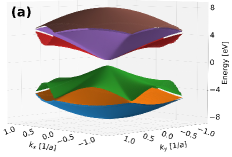
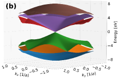
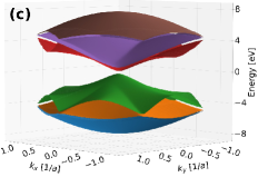
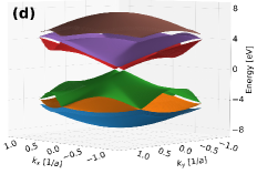
Figure 2: Energy dispersion for, a) Kek-O graphene, b) Kek-Y Graphene, c) Kek-O graphene with uniform strain in the $x$ direction ($\theta=0$), d) Kek-Y graphene with uniform strain in the $x$ direction. The plots were produced using $\Delta=0.05$ for all figures, and $\epsilon=0.03$ for c) and $\epsilon=0.05$ for d).

In Figure 2 we show a comparison between the energy dispersions for (a) graphene with a Kek-O pattern, (b) graphene with a Kek-Y pattern, (c) with a Kek-O pattern and strain, and (d) with a Kek-Y pattern and strain. From Fig. 2(a) and Fig. 2(c) it is clear that a gap is preserved for small values of $\epsilon$, although its size is considerable reduced when compared with the pure Kek-O pattern. This results from a competition between the Kekulé parameter that opens a gap and the magnitude of strain which closes it. Once the gap is closed, an increase of the strain results in two shifted Dirac cones (not shown).

Figure 2 (d) shows the results for a Kek-Y pattern with strain. Here, the effects of strain are much more important, as the central Dirac cones are no longer uniaxial, resulting in two separate Dirac cones. For this phase, strain preserves the massless character and moves the cones away from the center of the Brillouin zone. In Figure 1 we provide a short pictorial summary of the Dirac cones’ fate after applying a pure Kekulé, strain, or a Kekulé plus strain modulations. For the case of Kekulé plus strain, the tips of the two cones are much closer in reciprocal space than in the case of graphene. This suggests that strain can be used to control the distance between valleys to do valley engineering. As the electrical conductivityOliva2014 and the optical properties OlivaDicroism ; Oliva2016_PRB depend upon the distance in k-space of the cone tips, it is clear that strain valley engineering can be much more effective in Kekulé patterns than in pure graphene. In the following section, we will consider a low energy approximation that allows us to obtain a useful effective Dirac Hamiltonian for this system.

III Low-energy approximation

In order to obtain an effective Hamiltonian for low energies, we start by observing that the first row and column of the matrix $\Gamma$ given by Eq. 22 are negligible in such limit, since they correspond to the high energy bands depicted in brown and blue in Figure 2. As a result, we can redefine the column vector of annihilation operators as $u_{\bm{k}}=(a_{\bm{k}-\bm{G}^{\prime}},a_{\bm{k}+\bm{G}^{\prime}},b_{\bm{k}-\bm{G}^{\prime}},b_{\bm{k}+\bm{G}^{\prime}})$. The effective Hamiltonian now can be written as follows,

$$H_{Eff}=-u_{\bm{k}}^{\dagger}\begin{pmatrix}0&0&s^{\prime}_{-1}&\tilde{\Delta}s^{\prime}_{\nu}\\ 0&0&\tilde{\Delta}^{*}s^{\prime}_{-\nu}&s^{\prime}_{1}\\ s^{\prime*}_{-1}&\tilde{\Delta}s^{\prime*}_{-\nu}&0&0\\ \tilde{\Delta}^{*}s^{\prime*}_{\nu}&s^{\prime*}_{1}&0&0\\ \end{pmatrix}u_{\bm{k}}.$$ (25)

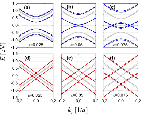
Figure 3: Energy dispersion relation around the $\Gamma$ point for Kekulé distorted graphene with parameter $\Delta=0.05$, and for different values of uniaxial strain along the $x$-axis ($\theta=0$). Panels (a-c) show the results for the Kek-O texture (blue curves) with $2.5\%$, $5\%$, and $7.5\%$ of strain, respectively. Panels (d-f) show (in red) the corresponding curves for the Kek-Y texture. The solid curves were obtained by solving numerically the Hamiltonian given by Eq.19, while the dashed curves were calculated by using the analytical expressions for the low energy approximation given by Eq. 30 and Eq. 34. The gray lines corresponds to the unstrained cases. Notice the good agreement between the numerical and low-energy approximation

.

Next, we proceed to expand Eq. 25 to first order in $\bm{k}$. To this end we can make an expansion of the energy dispersion $s^{\prime}_{n}$ around $n\bm{G}^{\prime}$. However, as other works have shown oliva-Leyva-PRB ; NaumisReview , it is necessary to expand around the true Dirac points, which are defined as the zeros of the deformed lattice energy dispersion, not located at the high-symmetry points of the strained-lattice, or at the original Dirac cones’ tips. These new Dirac points are given by $\bm{K}_{D}^{{}^{\prime}\pm}=\pm(\bm{G}^{\prime}+\bm{A})$, where $\bm{A}$ is the pseudo-magnetic vector potentialoliva-Leyva-PRB ; NaumisReview , whose explicit form depends upon the components of the strain tensor $\bar{\epsilon}$:

$$A_{x}=\frac{\beta}{2a}(\epsilon_{xx}-\epsilon_{yy}),\quad A_{y}=-\frac{\beta}{2a}(2\epsilon_{xy}).$$ (26)

By writing $s^{\prime}_{n}$ as $s^{\prime}(\bm{k}+n\bm{G}^{\prime}+n\bm{A}-n\bm{A})=s^{\prime}([\bm{k}-n\bm{A}]+n\bm{K}_{D}^{{}^{\prime}+})$ we can explicitly ensure that the expansion is performed around the true Dirac points. Then we return to $n\bm{G}^{\prime}$ through a translation of $-n\bm{A}$, such that

$$s^{\prime}_{n}\approx s^{\prime}(n\bm{K}_{D}^{{}^{\prime}+})+\nabla_{k}s^{\prime}(\bm{k})\rvert_{\bm{k}=n\bm{K}_{D}^{{}^{\prime}+}}\cdot(\bm{k}-n\bm{A})+O(\bm{k}^{2}).$$ (27)

Thus, the matrix elements of Eq. 25 can be expressed as follows:

$$s^{\prime}_{0}\approx 3\tilde{t_{0}}+iv_{f}a(\bm{A}\times\bm{p})_{z},$$ (28a)

$$s^{\prime}_{1}\approx-v_{f}[(\overline{p}_{x}-\hbar A_{x})-i[(\overline{p}_{y}-\hbar A_{y})],$$ (28b)

$$s^{\prime}_{-1}\approx v_{f}[(\overline{p}_{x}+\hbar A_{x})+i(\overline{p}_{y}+\hbar A_{y})],$$ (28c)

where $\tilde{t_{0}}=t_{0}[1-\frac{\beta\epsilon}{2}(1-\rho)]$, $\overline{\bm{p}}=(1+\bar{\epsilon}-\beta\bar{\epsilon})\bm{p}$, and we defined the Fermi velocity $v_{f}=3at_{0}/2\hbar$ as usual. Finally, we can write the Dirac-like equation for electrons in strained graphene with a Kekulé distorsion as,

$$\mathcal{H}\begin{pmatrix}\Psi_{-}\\ \Psi_{+}\end{pmatrix}=E\begin{pmatrix}\Psi_{-}\\ \Psi_{+}\end{pmatrix},$$ (29a)

$$\Psi_{-}=\begin{pmatrix}-\psi_{B,-}\\ \psi_{A,-}\\ \end{pmatrix},\quad\Psi_{+}=\begin{pmatrix}\psi_{A,+}\\ \psi_{B,+}\\ \end{pmatrix},$$ (29b)

$$\mathcal{H}=\begin{pmatrix}v_{f}\bm{\sigma}\cdot(\overline{\bm{p}}+\hbar\bm{A})&\tilde{\Delta}Q_{\nu}\\ \tilde{\Delta}^{*}Q_{\nu}^{\dagger}&v_{f}\bm{\sigma}\cdot(\overline{\bm{p}}-\hbar\bm{A})\end{pmatrix},$$ (29c)

$$Q_{\nu}=\left\{\begin{matrix}3\tilde{t_{0}}\sigma_{z}-iv_{f}a(\bm{A}\times\bm{p})_{z}\sigma_{0},&\nu=0\\ v_{f}[\nu\overline{p}_{x}-i\overline{p}_{y}]\sigma_{0}+\hbar v_{f}[A_{x}-i\nu A_{y}]\sigma_{z},&\nu=\pm 1\end{matrix}\right.,$$ (29d)

where $\psi_{s,v}$ is the wavefunction for sublattice $s\in\{A,B\}$ in the valley $v\in\{+,-\}$ and the Pauli matrices $\sigma_{i}$, $i\in\{0,x,y,z\}$ are acting in the pseudospin degree of freedom.

The energy eigenvalues of the Hamiltonian 29c can be obtained analytically for both Kekulé textures. For the Kek-O texture ($\nu=0$), we obtain the following expression,

$$E_{O,\pm}^{2}= v_{f}^{2}(|\overline{\bm{p}}|^{2}+\hbar^{2}\bm{|}A|^{2})+\Delta_{0}^{2}([3\tilde{t_{0}}]^{2}+[v_{f}a(\bm{A}\times\bm{p})_{z}]^{2})$$ (30)

$$\pm 2v_{f}\>\sqrt[]{v_{f}^{2}\hbar^{2}(\bm{A}\cdot\overline{\bm{p}})^{2}+\Delta_{0}^{2}(v_{f}^{2}a^{2}|\overline{\bm{p}}|^{2}(\bm{A}\times\bm{p})_{z}^{2}+2v_{f}\hbar a(3\tilde{t_{0}})(\bm{A}\times\bm{p})_{z}(\bm{A}\times\overline{\bm{p}})_{z}+\hbar^{2}(\tilde{3t_{0}})^{2}|\bm{A}|^{2})},$$

which recovers the result for the Kek-O unstrained grapheneGamayun and may be evaluated at ($k_{x},k_{y}$)=($0,0$) to find the condition for keeping the gapPark2015 ,

$$\epsilon<\frac{4|\Delta_{0}|}{\beta[(1+\rho)+2|\Delta_{0}|(1-\rho)]}$$ (31)

as well as its magnitude,

$$E_{Gap}=6t_{0}[|\Delta_{0}|-\frac{\beta\epsilon}{4}(1+\rho)-\frac{\beta\epsilon}{2}(1-\rho)|\Delta_{0}|]$$ (32)

This characterizes the competition between the Kekulé strength $\Delta_{0}$, and the magnitude of the applied strain $\epsilon$ to open and close the gap, and suggest a way to control this gap by strain. It has been pointed out that this gap becomes topologicalwakabayashi for negative values of $\Delta_{0}$. Notice that both equations are independent from the strain direction $\theta$, this is a consequence of the approximations made for small strain and low-energy. When the magnitude of strain equals the condition given by Eq. 31, the gap closes and the valence and conduction bands touches in just one point. For greater values of strain, the bands touch in two points (valleys) that split as strain increases. This is shown in the series of plots in Fig. 3(a)-3(b), where the dispersion relations around the center of the Brillouin zone for strained Kek-O graphene are presented. Gray lines are the dispersions for unstrained graphene with Kek-O texture. Blue continuous lines present the curves obtained numerically by calculating the eigenvalues of Eq.19 while dashed lines are the energies in the low energy approximation of Eq.30. They correspond to the eigenvalues of the effective Hamiltonian for the Kek-O texture given by,

$$\mathcal{H}_{O}= v_{f}\bm{\sigma}\cdot\overline{\bm{p}}\otimes\tau_{0}+\hbar v_{f}\bm{\sigma}\cdot\bm{A}\otimes\tau_{z}$$ (33)

$$+3\Delta_{0}t_{0}\sigma_{z}\otimes\tau_{x}+v_{\tau}a(\bm{A}\times\bm{p})_{z}\sigma_{0}\otimes\tau_{y},$$

where we have taken $\tilde{\Delta}=\Delta_{0}$, and used a second set of Pauli matrices $\tau_{x}$, $\tau_{y}$, $\tau_{z}$, with a unit matrix $\tau_{0}$ acting on valley space and defined the velocity $v_{\tau}=\Delta_{0}v_{f}$. Notice that the pseudomagnetic vector $\bm{A}$, as usual, appears as a momentum shift, nevertheless since it does not depend on space it can not give rise to a pseudomagnetic fieldvozmediano2010gauge ; AMORIM20161 ; NaumisReview .

For the Kek-Y texture ($\nu=\pm 1$), a gapless spectrum remains for all values of Keukulé and strain parameters, with energies given by,

$$E_{Y,\pm}^{2}= v_{f}^{2}(1+\Delta_{0}^{2})(|\overline{\bm{p}}|^{2}+\hbar^{2}|\bm{A}|^{2})$$ (34)

$$\pm\frac{v_{f}^{2}}{2}\,\sqrt[]{(1+\Delta_{0}^{2})^{2}(|\overline{\bm{p}}+\hbar\bm{A}|^{4}+|\overline{\bm{p}}-\hbar\bm{A}|^{4})-2|\overline{\bm{p}}+\hbar\bm{A}|^{2}|\overline{\bm{p}}-\hbar\bm{A}|^{2}(1-6\Delta_{0}^{2}+\Delta_{0}^{4})}.$$

In Fig. 3 we present a comparison between Eq. 30 and Eq. 34, with a calculation obtained from a numerical diagonalization of Eq. 19. The good agreement between both calculations validate our expressions for low-energy.

Finally, by taking $\nu=1$ and $\tilde{\Delta}=\Delta_{0}$, we obtain the low-energy effective Hamiltonian for the Kek-Y texture,

$$\mathcal{H}_{Y}= v_{f}\bm{\sigma}\cdot\overline{\bm{p}}\otimes\tau_{0}+\hbar v_{f}\bm{\sigma}\cdot\bm{A}\otimes\tau_{z}$$ (35)

$$+v_{\tau}\sigma_{0}\otimes\bm{\tau}\cdot\overline{\bm{p}}+\hbar v_{\tau}\sigma_{z}\otimes\bm{\tau}\cdot\bm{A}.$$

An equivalent expression is found for $\nu=-1$ and a complex $\tilde{\Delta}$.

When compared with the pure Kekulé effective Hamiltonian Gamayun , we observe two new terms, both containing $\bm{A}$. These two terms are $k$-independent and have a Zeeman-like structure, one in the pseudospin quantum number as it contains the product $\bm{\sigma}\cdot\bm{A}$, and the other in the valley quantum number (proportional to $\bm{\tau}\cdot\bm{A}$). The former is the leading term, since it depends linearly on $\epsilon$, while the latter depends on the product of $\epsilon\Delta$. Since the first term contains $\tau_{z}$, it splits the two valleys by moving each cone in opposite directions away from the center $\Gamma$ of the superlattice Brillouin zone, as shown in Fig.3 (d-f). The second term has a similar effect but in pseudospin space, nevertheless for modest values of strain and Kekulé distorsion it can be neglected. Although the first term is proportional to $\tau_{z}$ and the second is proportional to $\sigma_{z}$, both preserve the valley and pseudospin energy degeneracy.

IV Conclusions

We studied the effects upon the electronic properties of a space-independent strain in different types of Kekulé-patterns in graphene. For the Kek-O type, moderated values of strain preserve the gap although the size is changed. Above a certain strain threshold value, the gap closes leaving a two-Dirac-cones dispersion. For the Kek-Y type, strain splits the valleys along the direction of applied strain. However, as the valleys were folded before by the Kekulé pattern, it turns out that the distance in reciprocal space of the valleys is much closer than in pure graphene. This suggest that strain is useful to control the degree of intervalley scattering in Kekulé patterns. We also provided a low-energy Dirac effective Hamiltonian, which presents a Zeeman-like coupling between pseudospin and valleys to the pseudomagnetic vectorial potential.

References

- [1] John R Schaibley, Hongyi Yu, Genevieve Clark, Pasqual Rivera, Jason S Ross, Kyle L Seyler, Wang Yao, and Xiaodong Xu. Valleytronics in 2d materials. Nature Reviews Materials, 1(11):16055, 2016.
- [2] AH Castro Neto, F Guinea, Nuno MR Peres, Kostya S Novoselov, and Andre K Geim. The electronic properties of graphene. Reviews of modern physics, 81(1):109, 2009.
- [3] Chang-Yu Hou, Claudio Chamon, and Christopher Mudry. Electron fractionalization in two-dimensional graphenelike structures. Phys. Rev. Lett., 98:186809, May 2007.
- [4] Claudio Chamon. Solitons in carbon nanotubes. Phys. Rev. B, 62:2806–2812, Jul 2000.
- [5] Feng Liu, Minori Yamamoto, and Katsunori Wakabayashi. Topological edge states of honeycomb lattices with zero berry curvature. Journal of the Physical Society of Japan, 86(12):123707, 2017.
- [6] Long-Hua Wu and Xiao Hu. Topological properties of electrons in honeycomb lattice with detuned hopping energy. Scientific reports, 6:24347, 2016.
- [7] Kenjiro K Gomes, Warren Mar, Wonhee Ko, Francisco Guinea, and Hari C Manoharan. Designer dirac fermions and topological phases in molecular graphene. Nature, 483(7389):306, 2012.
- [8] Yizhou Liu, Chao-Sheng Lian, Yang Li, Yong Xu, and Wenhui Duan. Pseudospins and topological effects of phonons in a kekulé lattice. Phys. Rev. Lett., 119:255901, Dec 2017.
- [9] Zhuonan Lin, Wei Qin, Jiang Zeng, Wei Chen, Ping Cui, Jun-Hyung Cho, Zhenhua Qiao, and Zhenyu Zhang. Competing gap opening mechanisms of monolayer graphene and graphene nanoribbons on strong topological insulators. Nano Letters, 17(7):4013–4018, 2017. PMID: 28534404.
- [10] Sandro Sorella, Kazuhiro Seki, Oleg O. Brovko, Tomonori Shirakawa, Shohei Miyakoshi, Seiji Yunoki, and Erio Tosatti. Correlation-driven dimerization and topological gap opening in isotropically strained graphene. Phys. Rev. Lett., 121:066402, Aug 2018.
- [11] V.V. Cheianov, V.I. Fal’ko, O. Syljuåsen, and B.L. Altshuler. Hidden kekulé ordering of adatoms on graphene. Solid State Communications, 149(37):1499 – 1501, 2009.
- [12] Christopher Gutiérrez, Cheol-Joo Kim, Lola Brown, Theanne Schiros, Dennis Nordlund, Edward B Lochocki, Kyle M Shen, Jiwoong Park, and Abhay N Pasupathy. Imaging chiral symmetry breaking from kekulé bond order in graphene. Nature Physics, 12(10):950, 2016.
- [13] O V Gamayun, V P Ostroukh, N V Gnezdilov, İ Adagideli, and C W J Beenakker. Valley-momentum locking in a graphene superlattice with y-shaped kekulé bond texture. New Journal of Physics, 20(2):023016, 2018.
- [14] A Rycerz, J Tworzydło, and CWJ Beenakker. Valley filter and valley valve in graphene. Nature Physics, 3(3):172, 2007.
- [15] T. Fujita, M. B. A. Jalil, and S. G. Tan. Valley filter in strain engineered graphene. Applied Physics Letters, 97(4):043508, 2010.
- [16] Yongjin Jiang, Tony Low, Kai Chang, Mikhail I. Katsnelson, and Francisco Guinea. Generation of pure bulk valley current in graphene. Phys. Rev. Lett., 110:046601, Jan 2013.
- [17] J. Wang and S. Fischer. Topological valley resonance effect in graphene. Phys. Rev. B, 89:245421, Jun 2014.
- [18] Marko M. Grujić, Milan Ž. Tadić, and François M. Peeters. Spin-valley filtering in strained graphene structures with artificially induced carrier mass and spin-orbit coupling. Phys. Rev. Lett., 113:046601, Jul 2014.
- [19] Yafei Ren, Xinzhou Deng, Zhenhua Qiao, Changsheng Li, Jeil Jung, Changgan Zeng, Zhenyu Zhang, and Qian Niu. Single-valley engineering in graphene superlattices. Phys. Rev. B, 91:245415, Jun 2015.
- [20] R Carrillo-Bastos, C León, D Faria, A Latgé, Eva Y Andrei, and N Sandler. Strained fold-assisted transport in graphene systems. Physical Review B, 94(12):125422, 2016.
- [21] Thomas Stegmann and Nikodem Szpak. Current flow paths in deformed graphene: from quantum transport to classical trajectories in curved space. New Journal of Physics, 18(5):053016, 2016.
- [22] Gareth W Jones, Dario Andres Bahamon, Antonio H Castro Neto, and Vitor M Pereira. Quantized transport, strain-induced perfectly conducting modes, and valley filtering on shape-optimized graphene corbino devices. Nano letters, 17(9):5304–5313, 2017.
- [23] Qing-Ping Wu, Zheng-Fang Liu, Ai-Xi Chen, Xian-Bo Xiao, and Zhi-Min Liu. Full valley and spin polarizations in strained graphene with rashba spin orbit coupling and magnetic barrier. Scientific reports, 6, 2016.
- [24] Xian-Peng Zhang, Chunli Huang, and Miguel A Cazalilla. Valley hall effect and nonlocal transport in strained graphene. 2D Materials, 4(2):024007, 2017.
- [25] Mahmoud M. Asmar and Sergio E. Ulloa. Minimal geometry for valley filtering in graphene. Phys. Rev. B, 96:201407, Nov 2017.
- [26] Kun Luo, Tao Zhou, and Wei Chen. Probing the valley filtering effect by andreev reflection in a zigzag graphene nanoribbon with a ballistic point contact. Phys. Rev. B, 96:245414, Dec 2017.
- [27] C. W. J. Beenakker, N. V. Gnezdilov, E. Dresselhaus, V. P. Ostroukh, Y. Herasymenko, İ. Adagideli, and J. Tworzydło. Valley switch in a graphene superlattice due to pseudo-andreev reflection. Phys. Rev. B, 97:241403, Jun 2018.
- [28] Yee Sin Ang, Shengyuan A. Yang, C. Zhang, Zhongshui Ma, and L. K. Ang. Valleytronics in merging dirac cones: All-electric-controlled valley filter, valve, and universal reversible logic gate. Phys. Rev. B, 96:245410, Dec 2017.
- [29] Rory Brown, Niels R. Walet, and Francisco Guinea. Edge modes and nonlocal conductance in graphene superlattices. Phys. Rev. Lett., 120:026802, Jan 2018.
- [30] Mikkel Settnes, José Hugo García, and Stephan Roche. Valley-polarized quantum transport generated by gauge fields in graphene. arXiv preprint arXiv:1705.09085, 2017.
- [31] SP Milovanović and FM Peeters. Strained graphene hall bar. Journal of Physics: Condensed Matter, 29(7):075601, 2016.
- [32] Mikkel Settnes, Jose H Garcia, and Stephan Roche. Valley-polarized quantum transport generated by gauge fields in graphene. 2D Materials, 4(3):031006, 2017.
- [33] Ramon Carrillo-Bastos, Marysol Ochoa, Saúl A Zavala, and Francisco Mireles. Enhanced asymmetric valley scattering by scalar fields in non-uniform out-of-plane deformations in graphene. arXiv preprint arXiv:1806.04708, 2018.
- [34] Thomas Stegmann and Nikodem Szpak. Current splitting and valley polarization in elastically deformed graphene. arXiv preprint arXiv:1806.09576, 2018.
- [35] Dawei Zhai and Nancy Sandler. Local versus extended deformed graphene geometries for valley filtering. arXiv preprint arXiv:1806.11251, 2018.
- [36] Shu-guang Cheng, Haiwen Liu, Hua Jiang, Qing-Feng Sun, and X. C. Xie. Manipulation and characterization of the valley-polarized topological kink states in graphene-based interferometers. Phys. Rev. Lett., 121:156801, Oct 2018.
- [37] Di Xiao, Wang Yao, and Qian Niu. Valley-contrasting physics in graphene: Magnetic moment and topological transport. Phys. Rev. Lett., 99:236809, Dec 2007.
- [38] Di Xiao, Ming-Che Chang, and Qian Niu. Berry phase effects on electronic properties. Rev. Mod. Phys., 82:1959–2007, Jul 2010.
- [39] B. Amorim, A. Cortijo, F. de Juan, A.G. Grushin, F. Guinea, A. Gutiérrez-Rubio, H. Ochoa, V. Parente, R. Roldán, P. San-Jose, J. Schiefele, M. Sturla, and M.A.H. Vozmediano. Novel effects of strains in graphene and other two dimensional materials. Physics Reports, 617(Supplement C):1 – 54, 2016. Novel effects of strains in graphene and other two dimensional materials.
- [40] Gerardo G Naumis, Salvador Barraza-Lopez, Maurice Oliva-Leyva, and Humberto Terrones. Electronic and optical properties of strained graphene and other strained 2d materials: a review. Reports on Progress in Physics, 80(9):096501, 2017.
- [41] María AH Vozmediano, MI Katsnelson, and Francisco Guinea. Gauge fields in graphene. Physics Reports, 496(4):109–148, 2010.
- [42] RV Gorbachev, JCW Song, GL Yu, AV Kretinin, F Withers, Y Cao, A Mishchenko, IV Grigorieva, KS Novoselov, LS Levitov, et al. Detecting topological currents in graphene superlattices. Science, 346(6208):448–451, 2014.
- [43] Katsuyosih Komatsu, Yoshifumi Morita, Eiichiro Watanabe, Daiju Tsuya, Kenji Watanabe, Takashi Taniguchi, and Satoshi Moriyama. Observation of the quantum valley hall state in ballistic graphene superlattices. Science Advances, 4(5):eaaq0194, 2018.
- [44] N. Levy, S. A. Burke, K. L. Meaker, M. Panlasigui, A. Zettl, F. Guinea, A. H. Castro Neto, and M. F. Crommie. Strain-induced pseudo–magnetic fields greater than 300 tesla in graphene nanobubbles. Science, 329(5991):544–547, 2010.
- [45] Francisco Guinea, MI Katsnelson, and AK Geim. Energy gaps and a zero-field quantum hall effect in graphene by strain engineering. Nature physics, 6(1):30–33, 2010.
- [46] F. Guinea, A. K. Geim, M. I. Katsnelson, and K. S. Novoselov. Generating quantizing pseudomagnetic fields by bending graphene ribbons. Phys. Rev. B, 81:035408, Jan 2010.
- [47] L. González-Árraga, F. Guinea, and P. San-Jose. Modulation of kekulé adatom ordering due to strain in graphene. Phys. Rev. B, 97:165430, Apr 2018.
- [48] M. Oliva-Leyva and Gerardo G. Naumis. Understanding electron behavior in strained graphene as a reciprocal space distortion. Phys. Rev. B, 88:085430, Aug 2013.
- [49] Vitor M. Pereira, A. H. Castro Neto, and N. M. R. Peres. Tight-binding approach to uniaxial strain in graphene. Phys. Rev. B, 80:045401, Jul 2009.
- [50] M. Oliva-Leyva and Gerardo G. Naumis. Generalizing the fermi velocity of strained graphene from uniform to nonuniform strain. Physics Letters A, 379(40):2645 – 2651, 2015.
- [51] Andrés R. Botello-Méndez, Juan Carlos Obeso-Jureidini, and Gerardo G. Naumis. Toward an accurate tight-binding model of graphene’s electronic properties under strain. The Journal of Physical Chemistry C, 122(27):15753–15760, 2018.
- [52] M Oliva-Leyva and Gerardo G Naumis. Anisotropic ac conductivity of strained graphene. Journal of Physics: Condensed Matter, 26(12):125302, 2014.
- [53] M Oliva-Leyva and Gerardo G Naumis. Tunable dichroism and optical absorption of graphene by strain engineering. 2D Materials, 2(2):025001, 2015.
- [54] M. Oliva-Leyva and Gerardo G. Naumis. Effective dirac hamiltonian for anisotropic honeycomb lattices: Optical properties. Phys. Rev. B, 93:035439, Jan 2016.
- [55] Joon-Suh Park and Hyoung Joon Choi. Band-gap opening in graphene: A reverse-engineering approach. Phys. Rev. B, 92:045402, Jul 2015.
- [56] Christoph W Groth, Michael Wimmer, Anton R Akhmerov, and Xavier Waintal. Kwant: a software package for quantum transport. New Journal of Physics, 16(6):063065, 2014.