Measurements of $e^{+}e^{-}\to K_{S}^{0}K^{\pm}\pi^{\mp}\pi^{0}$ and $K_{S}^{0}K^{\pm}\pi^{\mp}\eta$ at center-of-mass energies from $3.90$ to $4.60~{}\mathrm{GeV}$

Abstract

Using $5.2\ \mathrm{fb}^{-1}$ $e^{+}e^{-}$ annihilation data samples collected with the BESIII detector, we measure the cross sections of $e^{+}e^{-}\to K_{S}^{0}K^{\pm}\pi^{\mp}\pi^{0}$ and $K_{S}^{0}K^{\pm}\pi^{\mp}\eta$ at center-of-mass energies from $3.90$ to $4.60$ GeV. In addition, we search for the charmonium-like resonance $Y(4260)$ decays into $K_{S}^{0}K^{\pm}\pi^{\mp}\pi^{0}$ and $K_{S}^{0}K^{\pm}\pi^{\mp}\eta$, and $Z_{c}^{0,\pm}(3900)$ decays into $K_{S}^{0}K^{\pm}\pi^{\mp,0}$ and $K_{S}^{0}K^{\pm}\eta$. Corresponding upper limits are provided since no clear signal is observed.

I Introduction

With the experimental progress in the past decade, many charmonium-like $(XYZ)$ states were observed, which can not be accommodated within the naive quark model and are proposed as the candidate of the hidden-charm exotic mesons XYZ_review1 ; XYZ_review2 . In this paper, we focus on the exotic states $Y(4260)$ and $Z_{c}(3900)$.

$Y(4260)$ was first observed in ISR process $e^{+}e^{-}\to\gamma_{\rm{ISR}}\pi^{+}\pi^{-}J/\psi$ by $BABAR$ PhysRevLett.95.142001 . In later experiments, $Y(4260)$ was also observed in $Y(4260)\to\pi^{0}\pi^{0}J/\psi$ Y4260_pi0jpsi . Recently, BESIII has observed a resonance around $4.23~{}\mathrm{GeV}$ in a open-charm process $e^{+}e^{-}\to\pi^{+}D^{0}D^{\star-}$ Y4260_piddstar . But no other open charm Y4260notseen1 ; Y4260notseen2 ; Y4260notseen3 ; Y4260notseen4 ; Y4260notseen5 ; Y4260notseen6 , hidden charm Y4260notseen7 ; Y4260notseen8 ; Y4260notseen9 and charmless Y4260notseen10 ; Y4260notseen11 ; Y4260notseen12 decay modes have be seen. Different interpretations were proposed to explain its structure, such as the charmonium states $4~{}^{3}{S_{1}}$ Y4260_4S_1 ; Y4260_4S_2 ; Y4260_4S_3 and $3~{}^{3}{D_{1}}$ Y4260_3D , hybrid charmonium Y4260_hybrid_1 ; Y4260_hybrid_2 , tetraquark state Y4260_4q_1 ; Y4260_4q_2 ; Y4260_4q_3 ; Y4260_4q_4 , molecular state Y4260_m_1 ; Y4260_m_2 ; Y4260_m_3 ; Y4260_m_4 ; Y4260_m_5 ; Y4260_m_6 , and non-resonance explanation Y4260_nonres1 ; Y4260_nonres2 ; Y4260_nonres3 .
The $Z_{c}(3900)$ was observed in the $J/\psi\pi^{\pm}$ invariant mass distribution of the $e^{+}e^{-}\to\pi^{+}\pi^{-}J/\psi$ process by the BESIII Collaboration PhysRevLett.110.252001 . Subsequently, additional $Z_{c}(3900)$ decay channels were observed, including $D\bar{D}^{*}+c.c$ PhysRevLett.112.022001 ; PhysRev.D92.092006 ; PhysRevLett.115.222002 , $D^{*}\bar{D}^{*}+c.c$ PhysRevLett.112.132001 ; PhysRevLett.115.182002 , and there are evidence for $Z_{c}(3900)$ decays into $\pi h_{c}$ PhysRevLett.111.242001 ; PhysRevLett.113.212002 . The $J^{P}$ of $Z_{c}(3900)$ was determined to be $1^{+}$ with a partial wave analysis of the $\pi^{+}\pi^{-}J/\psi$ final state Collaboration:2017njt . Since its discovery, many interpretations on the nature of the $Z_{c}(3900)$ have been proposed, such as a $D\bar{D}^{*}$ molecule ddmolecule , a tetra-quark state tetraquark , a cusp effect cusps , and dynamical generation through threshold effects threshold1 ; threshold2 .

Despite many interpretations, the natures of the $Y(4260)$ and $Z_{c}(3900)$ are still unclear. To comprehend these states, it is necessary to study more decay modes. All of the observed decay modes of the $Y(4260)$ and $Z_{c}(3900)$ are associated with the charm sector and no light hadron decay modes have been found yet lhd1 ; lhd2 ; PhysRev.D92.032009 . A search for light hadron decay modes of the $Y(4260)$ and $Z_{c}(3900)$ is complementary to previous studies and may help to distinguish between different theoretical models and to understand strong interaction effects in this energy region. Among the large number of potential light hadron decay modes, the branching fractions (BFs) of charmonium states decaying into $K_{S}K^{\pm}\pi^{\mp}\pi^{0}$ and $K_{S}K^{\pm}\pi^{\mp}\eta$ are usually large PDG . In four-body final state, there should be abundant intermediate states, which may supply more possible decay channels for searching $Y(4260)$ and $Z_{c}(3900)$. Furthermore, the existence of charged and neutral pions in the final states enable a study of isospin multiplets. In this paper, we present a measurement of the Born cross sections ($\sigma_{\rm{B}}$) for $e^{+}e^{-}\to K_{S}^{0}K^{\pm}\pi^{\pm}\pi^{0}$ and $K_{S}^{0}K^{\pm}\pi^{\mp}\eta$. We also report upper limits of $e^{+}e^{-}$ $\to$ $Y(4260)\to K_{S}^{0}K^{\pm}\pi^{\mp}\pi^{0}$, $e^{+}e^{-}$ $\to$ $Y(4260)\to K_{S}^{0}K^{\pm}\pi^{\mp}\eta$, $e^{+}e^{-}\to\pi^{\mp,0}Z_{c}(3900)^{\pm,0}\to K_{S}^{0}K^{\pm}\pi^{\mp}\pi^{0}$, and $e^{+}e^{-}\to\pi^{\mp}Z_{c}(3900)^{\pm}\to K_{S}^{0}K^{\pm}\pi^{\mp}\eta$.

II Detectors and Data samples

The BESIII detector Ablikim2010345 , operating at the BEPCII collider BEPCII , is a general purpose spectrometer with a geometrical acceptance of 93% of 4$\pi$ solid angle. It has four main components: (1) a small-cell, helium-based (60% He, 40% $\mbox{C}_{3}\mbox{H}_{8}$) multi-layer drift chamber (MDC) with 43 layers providing an average single-hit resolution of 135 $\mu$m, a momentum resolution of $0.5\%$ at 1.0 GeV/$c$ in a 1.0 T magnetic field, and a specific ionization energy loss ($dE/dx$) resolution better than 6%, (2) a time-of-flight (TOF) detector constructed of 5 cm thick plastic scintillators, with 176 strips of 2.4 m length in two layers in the barrel and 96 fans of the end-caps with time resolutions of 80 and 110 ps, respectively, which provide a 2$\sigma$ $K/\pi$ separation for momenta up to $\sim$ 1.0 GeV/$c$, (3) an electromagnetic calorimeter (EMC) consisting of 6240 CsI (Tl) crystals in a cylindrical barrel structure and two end-caps with an energy resolution of 2.5% (5%) at 1.0 GeV and a position resolution of 6 mm (9 mm) in the barrel (end-caps), and (4) a muon counter (MUC) consisting of resistive plate chambers (RPCs) in nine barrel and eight end-cap layers, which provide a 2 cm position resolution. More details of the BESIII detector can be found in Ref. Ablikim2010345 .

This analysis is based on $5.2\ \mathrm{fb}^{-1}$ $e^{+}e^{-}$ annihilation data samples Ablikim:2015nan collected with the BESIII detector at center-of-mass energies ($\sqrt{s}$) from 3.90 to 4.60 GeV Ablikim:2015zaa , which are listed in Table 1. Monte-Carlo (MC) simulations are used to optimize the event selection criteria, to study the detector acceptance and to understand the potential backgrounds. The geant4-based geant4 simulation software boost ref:boost is implemented to simulate the detector response, describe geometry and material, realize digitization, and incorporate time-dependent beam backgrounds. Six generic MC samples, equivalent to the integrated luminosity of the data at the energy points $4.009$, $4.230$, $4.260$, $4.360$, $4.420$ and $4.600$ $\mathrm{GeV}$ are generated to study the backgrounds. The primary known decay channels are generated using evtgen EVTGEN2 with the BFs set to the world average values PDG while the unknown decay modes are generated with lundcharm EVTGEN . Continuum hadronic events are generated with kkmc KKMC and QED processes such as Bhabha scattering, dimuon, and digamma events are generated with kkmc and babayaga Babayaga . To study the efficiency of each final state, a sample of $1\times 10^{5}$ signal events is generated at each energy point using kkmc, which simulates $e^{+}e^{-}$ annihilation, including beam energy spread and ISR effects.

III Data analysis

III.1 Measurement of $\sigma_{\rm{B}}(e^{+}e^{-}\to K_{S}^{0}K^{\pm}\pi^{\mp}\pi^{0})$ and $\sigma_{\rm{B}}(e^{+}e^{-}\to K_{S}^{0}K^{\pm}\pi^{\mp}\eta)$

Candidate events for $e^{+}e^{-}\to K_{S}^{0}K^{\pm}\pi^{\mp}\pi^{0}/\eta$, with $K_{S}^{0}\to\pi^{+}\pi^{-}$ and $\pi^{0}/\eta\to\gamma\gamma$ are selected according to the following steps. First, $K_{S}^{0}$ candidates are selected by looping over all pairs of oppositely charged tracks, which are assumed to be pions. Next, primary and secondary vertex fits SecondVFit are performed and the decay length of the secondary vertex fit is required to be greater than twice its uncertainty. Furthermore, the invariant mass of the pion pair is required to satisfy $|M(\pi^{+}\pi^{-})-M_{K_{S}^{0}}|<12$ MeV/$c^{2}$, where $M_{K_{S}^{0}}$ denotes the nominal mass of the $K_{S}^{0}$ PDG . If there are multiple $K_{S}^{0}$ candidates in one event, the one with the smallest $\chi^{2}$ from the secondary vertex fit is selected.

In addition to the two charged tracks that make up the $K_{S}^{0}$, two oppositely charged tracks are required. For the latter two charged tracks, the polar angle $\theta$ must satisfy $|\cos\theta|<0.93$ and the distance of closest approach to the interaction point must be less than $10.0~{}\mathrm{cm}$ and $1.0~{}\mathrm{cm}$ along the beam direction and in the plane perpendicular to the beam direction, respectively. The particle type for each charged track is determined by selecting the hypotheses with the highest probability, which is calculated with the combined information from TOF and $dE/dx$ measurements for different particle hypotheses. One charged track must be identified as a kaon and the other as a pion.

Photons are reconstructed from clusters deposited in the EMC, with the energy measured in the TOF included to improve reconstruction efficiency and energy resolution. At least two photons are required per event. The energy of a photon candidate is required to be larger than $25~{}\mathrm{MeV}$ in the barrel region ($|\cos\theta|<0.80$) or $50~{}\mathrm{MeV}$ in the end-cap region ($0.86<|\cos\theta|<0.92$). The cluster timing is required to be between $0$ and $700~{}\mathrm{ns}$ to suppress electronic noise and energy depositions unrelated to the event of interest. To eliminate showers associated with charged particles, the opening angle between a photon candidate and the extrapolated position of the closest charged track should be larger than $20$ degrees.

Finally, a four-constraint ($4\mathrm{C}$) kinematic fit imposing energy-momentum conservation is performed to the final states. Only events with $\chi^{2}_{\rm{4C}}<60$ are accepted. For events with more than two photon candidates, the photon pair with the smallest $\chi^{2}_{4\mathrm{C}}$ from the kinematic fit is accepted.

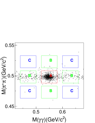
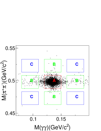
Figure 1: (Color online) The distributions of M($\pi^{+}\pi^{-}$) versus M($\gamma\gamma$) at $\sqrt{s}=4.258$ GeV. The top is the $\pi^{0}$ mode and the bottom is the $\eta$ mode. The boxes with mark “A” is the signal region and the boxes with mark “B” and “C” are sideband regions.

After the 4C kinematic fit, no peaking background is observed in the generic MC samples. The invariant mass distributions of $\pi^{+}\pi^{-}$ versus $\gamma\gamma$ at $4.258~{}\mathrm{GeV}$ are shown in Fig. 1 as an example in which obvious $K_{S}^{0}$ and $\pi^{0}/\eta$ peaks are observed. The signal regions are defined as $M(\pi^{+}\pi^{-})\in(0.488,0.508)~{}\mathrm{GeV}/c^{2}$, $M(\gamma\gamma)\in(0.12,0.15)~{}\mathrm{GeV}/c^{2}$ (for the $\pi^{0}$ mode) and $M(\gamma\gamma)\in(0.52,0.58)~{}\mathrm{GeV}/c^{2}$ (for the $\eta$ mode). The sideband regions are defined as $M(\pi^{+}\pi^{-})\in(0.463,0.483)\cup(0.513,0.533)~{}\mathrm{GeV}/c^{2}$, $M(\gamma\gamma)\in(0.08,0.11)\cup(0.16,0.19)~{}\mathrm{GeV}/c^{2}$ (for the $\pi^{0}$ mode) and $M(\gamma\gamma)\in(0.44,0.50)\cup(0.60,0.66)~{}\mathrm{GeV}/c^{2}$ (for the $\eta$ mode). The signal yields at each energy, presented in Tables 1 and 2, are obtained according to $N_{\rm{sig}}=N_{\rm{A}}-\sum N_{\rm{B}}/2+\sum N_{\rm{C}}/4$, where $N$ is the number of events and the subscript A denotes the signal region, and the subscripts B and C denote the sideband regions.

The Born cross section is calculated from

$$\sigma_{\rm{B}}=\frac{N_{\mathrm{sig}}}{\mathcal{L}\cdot\mathcal{B}\cdot\epsilon\cdot(1+\delta^{\mathrm{ISR}})\cdot\frac{1}{|1-\Pi(s)|^{2}}}\;,$$ (1)

where $\mathcal{L}$ is the integrated luminosity, $\epsilon$ is the detection efficiency, $\mathcal{B}$ is the product of the BF of $K_{S}^{0}\to\pi^{+}\pi^{-}$ and that of $\pi^{0}/\eta\to\gamma\gamma$  PDG , $\frac{1}{|1-\Pi(s)|^{2}}$ is the vacuum polarization correction factor VP , and $(1+\delta^{\rm{ISR}})$ is the ISR correction factor Kuraev:1985hb which is determined by the MC simulation programmer kkmc. The ISR factors are set to 1.0 to get the initial cross section lineshape as input to kkmc. From kkmc, the updated ISR factors are obtained, then the cross section lineshape is updated too. We repeat this process till both ISR factors and cross section converge.

The invariant mass distributions of any two or three final state particles at $\sqrt{s}=4.258~{}\rm{GeV}$ are shown in Figs. 2 and 3 as examples. There are some intermediate states observed in this four-body decay. To estimate the detection efficiency, a data-driven method is implemented to produce an exclusive MC sample that more closely resembles the data. This mixing MC sample includes intermediate resonances, such as $\rho(770)$ and $K^{*}(892)$, with couplings tuned to approximately match those appear in the data sample and is weighted according to the momentum distributions observed in the data sample. As illustrated in Figs. 2 and 3, the mixing MC sample gives a much better description of the data than a phase space (PHSP) MC sample. The observed cross sections are presented in Tables 1 and 2, and illustrated in Fig. 4.

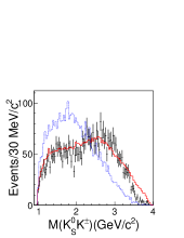
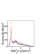
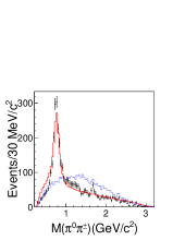
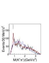
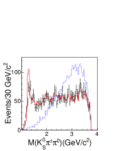
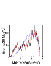
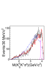
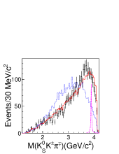
Figure 2: (Color online) Invariant mass distributions of any two or three final state particles for the $\pi^{0}$ mode at 4.258 GeV. The black dots with error bars are the data. The red solid lines are the mixing MC sample. The blue dashed lines are the PHSP MC sample. The pink dash-dotted lines in plot (i) and plot (j) are the MC shape of the $Z_{c}(3900)$ with an arbitrary scale.

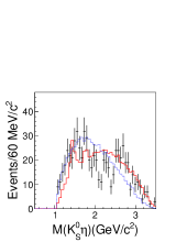
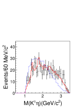
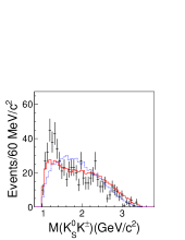
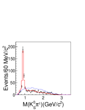
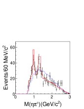
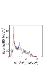
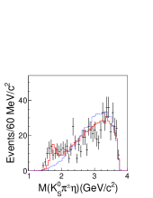
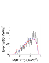
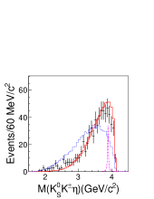
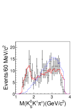
Figure 3: (Color online) Invariant mass distributions of any two or three final state particles for the $\eta$ mode at 4.258 GeV. The black dots with error bars are the data. The red solid lines are the mixing MC sample. The blue dashed lines are the PHSP MC sample. The pink dash-dotted line in plot (i) is the MC shape of the $Z_{c}(3900)$ with an arbitrary scale.

Table 1: Data sets and results of the Born cross section measurement for $e^{+}e^{-}\to K_{S}^{0}K^{\pm}\pi^{\mp}\pi^{0}$. The table includes the integrated luminosity $\mathcal{L}$, the number of observed signals events $N_{\rm{sig}}$, the efficiency $\epsilon$, the ISR correction factor $(1+\delta^{\rm{ISR}})$, the vacuum polarization correction factor $\frac{1}{|1-\Pi(s)|^{2}}$, and the Born cross section $\sigma_{\rm{B}}$. The first errors are statistical and the second ones are systematic. The details of systematic uncertainties are described in Sec. III.4.

$\sqrt{s}~{}(\mathrm{GeV})$	$\mathcal{L}~{}(\mathrm{pb^{-1}})$	$N_{\rm{sig}}$	$\epsilon~{}(\%)$	$(1+\delta^{\rm{ISR}})$	$\frac{1}{|1-\Pi(s)|^{2}}$	$\sigma_{\rm{B}}~{}(\mathrm{pb})$
3.896	52.61	$469\pm 22$	16.76	1.03	1.05	74.41 $\pm$ 3.47 $\pm$ 3.35
4.008	481.96	$3335\pm 58$	16.41	1.05	1.04	58.02 $\pm$ 1.01 $\pm$ 2.61
4.086	52.63	$~{}307\pm 18$	16.70	1.06	1.05	47.52 $\pm$ 2.73 $\pm$ 2.14
4.189	43.09	$~{}240\pm 16$	16.31	1.08	1.06	45.38 $\pm$ 2.94 $\pm$ 2.04
4.208	54.55	$~{}269\pm 17$	15.49	1.11	1.06	40.95 $\pm$ 2.50 $\pm$ 1.84
4.217	54.13	$~{}257\pm 16$	16.03	1.11	1.06	38.28 $\pm$ 2.40 $\pm$ 1.72
4.226	1091.74	$5235\pm 73$	15.90	1.10	1.06	39.23 $\pm$ 0.55 $\pm$ 1.77
4.242	55.59	$~{}255\pm 16$	16.02	1.10	1.06	37.46 $\pm$ 2.35 $\pm$ 1.69
4.258	825.67	$3850\pm 63$	15.52	1.12	1.05	38.65 $\pm$ 0.63 $\pm$ 1.74
4.308	44.90	$~{}199\pm 15$	15.55	1.11	1.05	36.86 $\pm$ 2.62 $\pm$ 1.66
4.358	539.84	$~{}2167\pm 47$	15.38	1.12	1.05	33.53 $\pm$ 0.72 $\pm$ 1.51
4.387	55.18	$~{}237\pm 16$	16.00	1.15	1.05	33.68 $\pm$ 2.20 $\pm$ 1.52
4.416	1073.56	$3934\pm 63$	15.21	1.14	1.05	30.38 $\pm$ 0.49 $\pm$ 1.37
4.467	109.94	$~{}378\pm 20$	15.87	1.17	1.06	26.70 $\pm$ 1.38 $\pm$ 1.20
4.527	109.98	$~{}364\pm 20$	15.35	1.17	1.06	26.51 $\pm$ 1.40 $\pm$ 1.19
4.575	46.67	$~{}149\pm 13$	15.15	1.19	1.06	24.87 $\pm$ 2.06 $\pm$ 1.12
4.600	566.93	$1612\pm 41$	15.49	1.16	1.06	22.71 $\pm$ 0.57 $\pm$ 1.02

Table 2: Same as TABLE 1 for $e^{+}e^{-}\to K_{S}^{0}K^{\pm}\pi^{\mp}\eta$.

$\sqrt{s}~{}(\mathrm{GeV})$	$\mathcal{L}~{}(\mathrm{pb^{-1}})$	$~{}~{}N_{\rm{sig}}$	$\epsilon~{}(\%)$	($1+\delta^{\rm{ISR}})$	$\frac{1}{|1-\Pi(s)|^{2}}$	$\sigma_{\rm{B}}~{}(\mathrm{pb})$
3.896	52.61	$76\pm 9$	18.22	1.02	1.05	$27.23\pm 3.22\pm 1.26$
4.008	481.96	$516\pm 24$	18.19	1.04	1.04	$19.88\pm 0.92\pm 0.94$
4.085	52.63	$~{}\,42\pm 7$	18.07	1.05	1.05	$14.71\pm 2.45\pm 0.70$
4.189	43.09	$~{}\,43\pm 7$	17.92	1.09	1.06	$17.75\pm 2.89\pm 0.84$
4.208	54.55	$~{}\,43\pm 7$	17.76	1.08	1.06	$14.20\pm 2.31\pm 0.61$
4.217	54.13	$~{}\,31\pm 6$	18.06	1.09	1.06	$10.05\pm 1.95\pm 0.41$
4.226	1091.74	$942\pm 31$	17.85	1.08	1.06	$15.61\pm 0.51\pm 0.64$
4.242	55.59	$~{}\,45\pm 7$	17.86	1.08	1.06	$14.63\pm 2.28\pm 0.60$
4.258	825.67	$655\pm 26$	17.75	1.08	1.05	$14.35\pm 0.57\pm 0.66$
4.308	44.90	$~{}\,32\pm 6$	17.59	1.12	1.05	$12.67\pm 2.38\pm 0.55$
4.358	539.84	$349\pm 19$	17.79	1.12	1.05	$11.38\pm 0.62\pm 0.51$
4.387	55.18	$~{}\,40\pm 6$	17.44	1.11	1.05	$13.05\pm 1.96\pm 0.62$
4.416	1073.56	$638\pm 26$	17.56	1.11	1.05	$10.62\pm 0.43\pm 0.49$
4.467	109.94	$~{}\,66\pm 8$	17.23	1.14	1.06	$10.62\pm 1.29\pm 0.52$
4.527	109.98	$~{}\,45\pm 7$	17.20	1.14	1.06	$~{}\,7.27\pm 1.31\pm 0.37$
4.575	47.67	$~{}\,27\pm 5$	17.29	1.15	1.06	$~{}\,9.23\pm 1.84\pm 0.49$
4.600	566.93	$288\pm 18$	17.20	1.18	1.06	$~{}\,8.67\pm 0.54\pm 0.43$

III.2 Upper limits of $e^{+}e^{-}$ $\to$ $Y(4260)$ $\to$ $K_{S}^{0}$$K^{\pm}$$\pi^{\mp}$$\pi^{0}$ and $e^{+}e^{-}$ $\to$ $Y(4260)$ $\to$ $K_{S}^{0}$$K^{\pm}$$\pi^{\mp}$$\eta$

Since there is no obvious structure in the line shapes of the Born cross sections for $e^{+}e^{-}\to K_{S}^{0}K^{\pm}\pi^{\mp}\pi^{0}$ and $e^{+}e^{-}\to K_{S}^{0}K^{\pm}\pi^{\mp}\eta$, as shown in Fig. 4, the upper limits of $Y(4260)$ $\to$ $K_{S}^{0}$ $K^{\pm}$ $\pi^{\mp}$ $\pi^{0}$ and $Y(4260)$ $\to$ $K_{S}^{0}$ $K^{\pm}$ $\pi^{\mp}$ $\eta$ are determined by fitting the line shapes with the function $\sigma_{\rm{B}}(\sqrt{s})=c_{0}\cdot{f(\sqrt{s})}+\rm{BW(\sqrt{s})}$. Here $f(\sqrt{s})=\frac{p_{0}}{(\sqrt{s})^{p_{1}}}$ describes the continuum process $e^{+}e^{-}\to K_{S}^{0}K^{\pm}\pi^{\mp}\pi^{0}/\eta$, the parameters $p_{0}$ and $p_{1}$ are determined by fitting the line shapes with only the continuum process. $\rm BW(\sqrt{s})$ given in Eq. (2)

$$\rm{BW(\sqrt{s})}=\frac{12\pi\Gamma_{\rm{e^{+}e^{-}}}\mathcal{B}\Gamma_{tot}}{(s-M^{2})^{2}+M^{2}\Gamma_{tot}^{2}}$$ (2)

is a relativistic Breit-Wigner function describing the resonance $Y(4260)$, where $\rm M$, $\Gamma_{\rm{tot}}$, and $\Gamma_{\rm{e^{+}e^{-}}}$ are the mass, full width, and electronic width of $Y(4260)$, respectively; $\mathcal{B}$ is the branching fraction of the decay $Y(4260)$ $\to$ $K_{S}^{0}$ $K^{\pm}$ $\pi^{\mp}$ $\pi^{0}/\eta$.
The mass and the full width of Y(4260) are set to the world average values $4230\pm 8~{}\mathrm{MeV/c^{2}}$ and $55\pm 19~{}\mathrm{MeV/c^{2}}$ PDG . The parameter $c_{0}$ is allowed to float during the fits, while the product $\Gamma_{\rm{e^{+}e^{-}}}\mathcal{B}$ increases from $0$ to $0.5$ $\mathrm{eV}$ in step length of $0.001~{}\mathrm{eV}$. For each value of it, a fitting estimator $Q^{2}$ defined by Eq. (3)

$$Q^{\rm{2}}=\sum\limits_{i}\frac{(\sigma_{\rm{B}_{i}}-h\cdot\sigma_{\rm{B}_{i}}^{\rm{fit}})^{2}}{\delta_{i}^{2}}+\frac{(h-1)^{2}}{\delta_{c}^{2}}$$ (3)

is obtained. Here $\sigma_{\rm{B}}$ and $\sigma_{\rm{B}}^{\rm{fit}}$ are the measured and fitted Born cross sections, $\delta_{i}$ is the energy dependent part of the total uncertainty, which includes the statistical uncertainty and the energy dependent part of systematic uncertainty, the $\delta_{c}$ is the energy independent part of the systematic uncertainty (the systematic uncertainties are described in detail in Sec. III.4), $h$ is a free parameter introduced to take into account the correlation of different energy points, and the subscript $i$ indicates the index of each energy point estimator . The $Q^{2}$ is used to calculate the likelihood $L$ = $e^{-0.5Q^{2}}$, whose normalized distribution is used to get the upper limits of $\Gamma_{\rm{e^{+}e^{-}}}\mathcal{B}$ at the $90\%$ confidence level (C.L.), which is determined to be $0.050~{}\mathrm{eV}$ and $0.19~{}\mathrm{eV}$ for the $\pi^{0}$ mode and the $\eta$ mode, respectively.

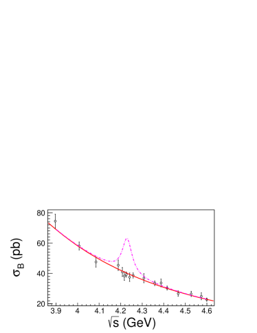
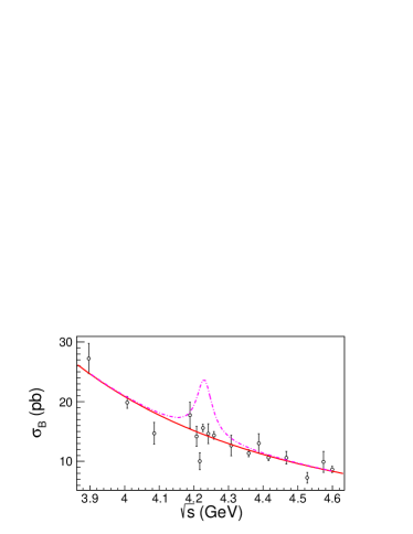
Figure 4: (Color Online) Line shapes of Born cross sections for $e^{+}e^{-}\rightarrow K_{S}^{0}K\pi\pi^{0}$ (a), and $e^{+}e^{-}\rightarrow K_{S}^{0}K\pi\eta$ (b). The dots with error bars are the measured Born cross sections. The solid red lines are the fitted results with the function $f(\sqrt{s})=\frac{p_{0}}{(\sqrt{s})^{p_{1}}}$ and parameters $p_{0}=(6.14\pm 1.54)\times 10^{6}~{}\mathrm{(pb)}\cdot(\mathrm{GeV})^{p_{1}}$ and $p_{1}=6.68\pm 0.17$ in the $\pi^{0}$ mode and $p_{0}=(1.86\pm 0.97)\times 10^{5}~{}\mathrm{(}pb)\cdot\mathrm{(GeV)}^{p_{1}}$ and $p_{1}=6.56\pm 0.36$ in the $\eta$ mode. The pink dash-dotted lines are the MC shape of the $Y(4260)$ with an arbitrary scale factor.

III.3 Upper limits on $\sigma_{\rm{B}}$$\big{(}$$e^{+}e^{-}$ $\to$ $\pi^{0,\mp}$ $Z^{0,\pm}_{c}(3900)$, $Z^{0,\pm}_{c}(3900)$ $\to$ $K_{S}^{0}$$K^{\pm}$$\pi^{\mp,0}/\eta$$\big{)}$

Since there is no obvious $Z_{c}(3900)$ signal in the invariant mass distributions of $K_{S}^{0}K^{\pm}\pi^{\mp,0}$ ($\pi^{0}$ mode) and $K_{S}^{0}K^{\pm}\eta$ ($\eta$ mode), as shown in Figs. 2 and 3, the upper limits at the $90\%$ C.L. for the production cross section $\sigma_{\rm{B}}\big{(}$$e^{+}e^{-}$ $\to$ $\pi$ $Z_{c}(3900)\big{)}$, with $Z_{c}(3900)$ $\to$ $K_{S}^{0}$ $K$ $\pi/\eta$ are determined with an unbinned maximum likelihood fit to the invariant mass of $K_{S}^{0}K\pi/\eta$ in the range $(3.7,4.1)~{}\mathrm{GeV}/c^{2}$, at the five energy points $4.226$, $4.258$, $4.358$, $4.416$, and $4.600$ $\mathrm{GeV}$. The contribution of non-$K_{S}^{0}$ or non-$\pi^{0}/\eta$ backgrounds is negligible. In the fit, the $Z_{c}(3900)$ signal is described by the MC simulated shape, and the mass and width of the $Z_{c}(3900)$ are set to theirs world average value $3886.6\pm 2.4$ $\mathrm{MeV}/c^{2}$ and $28.2\pm 2.6$ $\mathrm{MeV}/c^{2}$ PDG , respectively. The background is described by a second order polynomial function. The normalized likelihood distribution of the Born cross section $L(\sigma_{\rm{B}})$ is determined by changing the number of signal events from $0$ to $150$ with a step size of $1$. The upper limit (UL) at the $90\%$ C.L. is calculated by solving the equation

$$0.1=\int_{\rm{UL}}^{\infty}L(\sigma_{\rm{B}})d\sigma_{\rm{B}}\;,$$ (4)

The final upper limits are shown in Table 3, where all of the systematic uncertainties have been considered, the details of which are explained in Sec. III.4. The ratio

$$R=\frac{\sigma_{B}(e^{+}e^{-}\to\pi Z_{c}(3900)\to\pi K_{S}^{0}K\pi/\eta)}{\sigma_{B}(e^{+}e^{-}\to\pi Z_{c}(3900)\to\pi\pi J/\psi)}$$

is also given in Table 3, where the cross sections for $e^{+}e^{-}$ $\to$ $\pi^{\mp}Z_{c}(3900)^{\pm}\to\pi^{+}\pi^{-}J/\psi$ and $e^{+}e^{-}$ $\to$ $\pi^{0}Z_{c}(3900)^{0}\to\pi^{0}\pi^{0}J/\psi$ are from Ref. Collaboration:2017njt and Ref. PhysRevLett.115.112003 , respectively.

Table 3: Upper limits on $\sigma_{\rm{B}}\big{(}$$e^{+}e^{-}$ $\rightarrow$ $\pi$$Z_{c}(3900)$, $Z_{c}(3900)$$\to$$K_{S}^{0}$$K$$\pi/\eta\big{)}$, and its ratio (R) to $\sigma_{\rm{B}}(e^{+}e^{-}\to\pi Z_{c}(3900),\ Z_{c}(3900)\to\pi J/\psi)$ at the 90% C.L..

	$\sqrt{s}~{}(\rm{GeV})$	$\sigma_{\rm{B}}~{}(\mathrm{pb})$	R
$e^{+}e^{-}\rightarrow\pi^{0}Z_{c}(3900)^{0},$	4.226	$<0.24$	$<2.5\times 10^{-2}$
$Z_{c}(3900)^{0}\to K_{S}^{0}K^{\pm}\pi^{\mp}$	4.258	$<0.38$	$<1.2\times 10^{-1}$
	4.358	$<0.51$	$<2.6\times 10^{-1}$
	4.416	$<0.27$	-
	4.600	$<0.33$	-
$e^{+}e^{-}\rightarrow\pi^{\pm}Z_{c}(3900)^{\mp},$	4.226	$<0.17$	$<9.1\times 10^{-3}$
$Z_{c}(3900)^{\mp}\to K_{S}^{0}K^{\mp}\pi^{0}$	4.258	$<0.28$	$<5.6\times 10^{-2}$
	4.358	$<0.57$	-
	4.416	$<0.34$	-
	4.600	$<0.45$	-
$e^{+}e^{-}\rightarrow\pi^{\pm}Z_{c}(3900)^{\mp},$	4.226	$<0.18$	$<1.0\times 10^{-2}$
$Z_{c}(3900)^{\mp}\to K_{S}^{0}K^{\mp}\eta$	4.258	$<0.56$	$<1.4\times 10^{-1}$
	4.358	$<0.53$	-
	4.416	$<0.76$	-
	4.600	$<0.58$	-

III.4 Systematic Uncertainties

Various sources of systematic uncertainty are investigated in the $K_{S}^{0}K^{\pm}\pi^{\mp}\pi^{0}$ and $K_{S}^{0}K^{\pm}\pi^{\mp}\eta$ lineshape measurement. We assume that the systematic uncertainties associated with the physics model used in the MC simulation, the luminosity, tracking, PID, $\gamma$ reconstruction efficiency, $K^{0}_{S}$ reconstruction efficiency, ISR correction factor, vacuum polarization factor and quoted BFs are energy independent, while the other systematic effects are energy dependent.

For the $\pi^{0}$ mode, a data-driven MC method is developed to obtain the efficiency. To estimate the uncertainty of this method, one thousand testing samples of $e^{+}e^{-}\to K_{S}^{0}K^{\pm}\pi^{\mp}\pi^{0}$ are generated with eighteen different physics processes with random ratios, the ratio of each process is generated using uniform distribution between 0 to 1 and then normalized by the summation of these eighteen ratios. The difference between the estimated and the real efficiencies is fitted with a Gaussian function. The fit results give a mean of $0.4\%$ which is neglected, and a width of $0.9\%$ which is taken as the systematic uncertainty from the data-driven MC method. For the $\eta$ mode, which has much lower statistics than the $\pi^{0}$ mode, alternative mixing ratios are used to generate a new MC sample and the efficiency difference between the two MC samples is adopted as the systematic uncertainty.

The uncertainty on the integrated luminosity is estimated to be $1.0\%$ using Bhabha events Ablikim:2015nan .

Both the uncertainties of tracking and PID for charged tracks originating at the interaction point are determined to be $1.0\%$ per track using $J/\psi\to K_{S}^{0}K^{\pm}\pi^{\mp}$, $J/\psi\to p\bar{p}\pi^{+}\pi^{-}$, and $J/\psi\to\pi^{+}\pi^{-}\pi^{0}$ Ablikim:2011kv as control samples.

The uncertainty due to photon reconstruction efficiency is $1.0\%$ per photon, which is derived from studies of $J/\psi\to\rho^{0}\pi^{0},\rho^{0}\to\pi^{+}\pi^{-},\pi^{0}\to\gamma\gamma$ pi0_rec_eff .

The uncertainty associated with the $K_{S}^{0}$ reconstruction is studied using $J/\psi\rightarrow K^{*}(892)^{\pm}K^{\mp},K^{*}(892)^{\pm}\to K_{S}^{0}\pi^{\pm}$ and $J/\psi\rightarrow\phi K_{S}^{0}K^{\pm}\pi^{\mp}$ control samples and is estimated to be 1.2% Ks_err .

The ISR correction factor introduces a $1.0\%$ uncertainty since the termination condition of the recursion method used to get the correction factor is $1.0\%$ between the last two iterations.

The uncertainty due to the vacuum polarization factor is found to be negligible VP . The uncertainties of the quoted BFs are also considered.

The energy dependent ones include the systematic uncertainties from the choosing about mass window and sideband regions of $K_{S}^{0}$, $\pi^{0}$, and $\eta$ and the kinematic fit. The uncertainties associated with the $K_{S}^{0}$, $\pi^{0}$, and $\eta$ invariant mass regions are determined by changing them from $(0.488,0.508)$ to $(0.483,0.513)~{}\mathrm{GeV}/c^{2}$, $(0.12,0.15)$ to $(0.115,0.155)~{}\mathrm{GeV}/c^{2}$ and $(0.52,0.58)$ to $(0.51,0.59)~{}\mathrm{GeV}/c^{2}$ for the $K_{S}^{0}$, $\pi^{0}$ and $\eta$, respectively. The differences in the efficiencies are taken as the corresponding systematic uncertainties.

The uncertainties due to the side-band regions are determined by changing the side-band region to $M_{\eta}\in(0.44,0.47)\cup(0.63,0.66)~{}\mathrm{GeV}/c^{2}$, $M_{\pi^{0}}\in(0.08,0.095)\cup(0.175,0.19)~{}\mathrm{GeV}/c^{2}$ and $M_{K_{S}^{0}}\in(0.463,0.473)\cup(0.523,0.533)~{}\mathrm{GeV}/c^{2}$. The differences are taken as the associated systematic uncertainties.

The uncertainty associated with the kinematic fit is determined by comparing the efficiencies with and without corrections to the track helix parameters Ablikim:2012pg .

Assuming all sources of systematic uncertainties are independent, the total uncertainties are the sums of the individual values in quadrature (Table 4).

Table 4: Summary of systematic uncertainties (in %).

	$\sqrt{s}~{}(\rm{GeV})$	$3.896$	$4.008$	$4.085$	$4.189$	$4.208$	$4.217$	$4.226$	$4.242$	$4.258$	$4.308$	$4.358$	$4.387$	$4.416$	$4.467$	$4.527$	$4.575$	$4.600$
both mode	$\mathcal{L}$	1.0	1.0	1.0	1.0	1.0	1.0	1.0	1.0	1.0	1.0	1.0	1.0	1.0	1.0	1.0	1.0	1.0
	$K_{S}^{0}$ reconstruction	1.2	1.2	1.2	1.2	1.2	1.2	1.2	1.2	1.2	1.2	1.2	1.2	1.2	1.2	1.2	1.2	1.2
	Tracking	2.0	2.0	2.0	2.0	2.0	2.0	2.0	2.0	2.0	2.0	2.0	2.0	2.0	2.0	2.0	2.0	2.0
	PID	2.0	2.0	2.0	2.0	2.0	2.0	2.0	2.0	2.0	2.0	2.0	2.0	2.0	2.0	2.0	2.0	2.0
	$\gamma$ reconstruction	2.0	2.0	2.0	2.0	2.0	2.0	2.0	2.0	2.0	2.0	2.0	2.0	2.0	2.0	2.0	2.0	2.0
	$\rm{BF}_{K_{S}^{0}\rightarrow\pi^{+}\pi^{-}}$	0.1	0.1	0.1	0.1	0.1	0.1	0.1	0.1	0.1	0.1	0.1	0.1	0.1	0.1	0.1	0.1	0.1
	$(1+\delta^{ISR})$	1.0	1.0	1.0	1.0	1.0	1.0	1.0	1.0	1.0	1.0	1.0	1.0	1.0	1.0	1.0	1.0	1.0
$\pi^{0}$ mode	Mixing MC	0.9	0.9	0.9	0.9	0.9	0.9	0.9	0.9	0.9	0.9	0.9	0.9	0.9	0.9	0.9	0.9	0.9
	Kinematic fit	0.3	0.3	0.3	0.3	0.3	0.4	0.3	0.3	0.4	0.1	0.2	0.2	0.2	0.4	0.4	0.3	0.4
	$\pi^{0}$ mass interval	0.6	0.6	0.6	0.6	0.6	0.6	0.6	0.6	0.5	0.5	0.6	0.6	0.6	0.6	0.8	0.8	0.8
	$K_{S}^{0}$ mass interval	0.1	0.1	0.1	0.1	0.1	0.1	0.1	0.1	0.3	0.3	0.2	0.3	0.3	0.3	0.2	0.2	0.2
	side-band	0.2	0.2	0.2	0.2	0.1	0.1	0.1	0.1	0.1	0.1	0.1	0.1	0.1	0.1	0.1	0.1	0.1
	$\rm{BF}_{\pi^{0}\rightarrow\gamma\gamma}$	0.1	0.1	0.1	0.1	0.1	0.1	0.1	0.1	0.1	0.1	0.1	0.1	0.1	0.1	0.1	0.1	0.1
	Total	4.1	4.1	4.1	4.1	4.1	4.1	4.1	4.1	4.1	4.1	4.1	4.1	4.1	4.1	4.1	4.1	4.1
$\eta$ mode	Mixing MC	0.2	1.4	1.1	1.0	1.2	0.3	0.1	0.4	1.6	0.5	1.4	1.2	0.3	1.6	1.5	0.6	0.9
	Kinematic fit	0.3	0.2	0.2	0.2	0.2	0.2	0.2	0.3	0.3	0.2	0.1	0.3	0.4	0.1	0.2	0.2	0.2
	$\eta$ mass interval	1.6	1.6	1.6	1.6	0.6	0.6	0.6	0.6	0.9	0.9	1.0	0.4	0.4	0.4	1.7	1.7	1.7
	$K_{S}^{0}$ mass interval	1.7	1.7	1.7	1.7	0.7	0.7	0.7	0.7	1.4	1.4	1.1	2.1	2.1	2.1	2.3	2.3	2.3
	side-band	0.1	0.1	0.1	0.1	0.6	0.6	0.6	0.6	0.5	0.5	0.4	1.1	1.1	1.1	0.4	0.4	0.4
	$\rm{BF}_{\eta\rightarrow\gamma\gamma}$	0.5	0.5	0.5	0.5	0.5	0.5	0.5	0.5	0.5	0.5	0.5	0.5	0.5	0.5	0.5	0.5	0.5
	Total	4.6	4.8	4.7	4.7	4.3	4.1	4.1	4.1	4.6	4.4	4.5	4.8	4.7	4.9	5.1	4.9	5.0

The systematic uncertainties that affect the upper limits on $\sigma_{\rm{B}}\big{(}e^{+}e^{-}\to\pi Z_{c}(3900),Z_{c}(3900)\to K_{S}^{0}K\pi/\eta\big{)}$ are considered in two categories: multiplicative and non-multiplicative. The non-multiplicative systematic uncertainties on the signal shape and the background shape are considered by changing the signal shape to a Breit-Wigner function and varying the fit range, the parameters of the $Z_{c}(3900)$, and the order of the polynomial functions in the fit. The maximum upper limits are adopted for all combinations of these variations. The intermediate states in the $Z_{c}(3900)$ decay are considered by generating signal MC samples with alternative processes $Z_{c}(3900)\to K^{*}(892)K$, $K^{*}(892)\to K(K_{S}^{0})\pi$ ($\pi^{0}$ mode), and $Z_{c}(3900)\to a_{0}(980)\eta$, $a_{0}(980)\to K_{S}^{0}K$ ($\eta$ mode). The efficiency difference is considered as a multiplicative systematic uncertainty. All of the systematic uncertainties, which are listed in Table 4, excluding the side-band item and mixing MC item, are considered as the multiplicative systematic uncertainties. The effects of multiplicative systematic uncertainties are taken into account by convolving the distribution of $L(\sigma_{\rm{B}})$ with a probability distribution function of sensitivity $(S)$, which is assumed to be a Gaussian function with central value $\hat{S}$ and standard deviation $\delta_{S}$ smear :

$$L^{\prime}(\sigma_{\rm{B}})=\int_{0}^{1}L(\frac{S}{\hat{S}}\sigma_{\rm{B}})\cdot e^{-\frac{(S-\hat{S})^{2}}{2\delta_{\sc{s}}^{2}}}dS\;.$$ (5)

Here $S$ is the sensitivity that refers to the denominator of Eq. (1) and $\delta_{\sc{s}}$ is the total multiplicative systematic uncertainty. $L^{\prime}(\sigma_{\rm{B}})$ is the likelihood distribution of the Born cross section after the multiplicative systematic uncertainties are incorporated.

IV Summary

The Born cross sections for $e^{+}e^{-}\to K_{S}^{0}K^{\pm}\pi^{\mp}\pi^{0}$ and $K_{S}^{0}K^{\pm}\pi^{\mp}\eta$ are measured with data samples collected at center-of-mass energies from $3.90$ to $4.60~{}\mathrm{GeV}$. Since no clear structure is observed, the upper limits of the product $\Gamma_{\rm{e^{+}e^{-}}}\mathcal{B}$ $\big{(}$ $Y(4260)$ $\to$$K_{S}^{0}$$K^{\pm}$$\pi^{\mp}$$\pi^{0}$$\big{)}$ at $90\%$ C.L. is estimated to be less than $0.05~{}\mathrm{eV}$ and that of $\Gamma_{\rm{e^{+}e^{-}}}{\mathcal{B}}\big{(}Y(4260)\to$$K_{S}^{0}$$K^{\pm}$$\pi^{\mp}$$\eta$$\big{)}$ is estimated to be smaller than $0.19~{}\mathrm{eV}$. Ref. Ablikim:2016qzw reported four solutions of the product $\Gamma_{\rm{e^{+}e^{-}}}\mathcal{B}\big{(}Y(4260)\to$ $\pi^{+}\pi^{-}J/\psi\big{)}$, in which the maximum is $13.3\pm 1.4~{}\mathrm{eV}$ and the minimum is $1.5\pm 0.3~{}\mathrm{eV}$. Comparing them with our results, the branching fraction of the $Y(4260)$ decaying into $K_{S}^{0}K^{\pm}\pi^{\mp}\pi^{0}$ and $K_{S}^{0}K^{\pm}\pi^{\mp}\eta$ is much smaller, which indicates a much smaller coupling of the $Y(4260)$ to the light hadrons $K_{S}^{0}$$K^{\pm}$$\pi^{\mp}$$\pi^{0}$ and $K_{S}^{0}$$K^{\pm}$$\pi^{\mp}$$\eta$. We also search for $e^{+}e^{-}\to\pi Z_{c}(3900),\ Z_{c}(3900)\to K_{S}^{0}K\pi/\eta$ and no obvious $Z_{c}(3900)$ signal is observed in the charged nor neutral mode. The 90% C.L. upper limits on the cross sections are given at $\sqrt{s}=$ $4.226$, $4.258$, $4.358$, $4.416$, and $4.600~{}\mathrm{GeV}$. The absence of a signal suggests that the cross sections for light hadron decay modes are small and that the annihilation of $c\bar{c}$ in the $Y(4260)$ and $Z_{c}(3900)$ is suppressed. Additional exploration of light hadron decay modes is needed to confirm the hypotheses.