Pion electromagnetic form factor at high precision with implications to $a_{\mu}^{\pi\pi}$ and the onset of perturbative QCD

Abstract

We extend recently developed methods used for determining the electromagnetic charge radius and $a_{\mu}^{\pi\pi}$ to obtain a determination of the electromagnetic form factor of the pion, $F_{\pi}^{V}(t)$, in several significant kinematical regions, using a parametrization-free formalism based on analyticity and unitarity, with the inclusion of precise inputs from both timelike and spacelike regions. On the unitarity cut, below the first inelastic threshold, we use the precisely known phase of the form factor, known from $\pi\pi$ elastic scattering via the Fermi-Watson theorem, and above the inelastic threshold a conservative integral condition on the modulus. We also use as input the experimental values of the modulus at several energies in the elastic region, where the data from $e^{+}e^{-}\to\pi^{+}\pi^{-}$ and $\tau$ hadronic decays are mutually consistent, as well as the most recent measurements at spacelike momenta. The experimental uncertainties are implemented by Monte Carlo simulations. At spacelike values $Q^{2}=-t>0$ near the origin, our predictions are consistent and significantly more precise than the recent QCD lattice calculations. The determinations at larger $Q^{2}$ confirm the late onset of perturbative QCD for exclusive quantities. From the predictions of $|F_{\pi}^{V}(t)|^{2}$ on the timelike axis below 0.63 GeV, we obtain the hadronic vacuum polarization (HPV) contribution to the muon anomaly, $a_{\mu}^{\pi\pi}|_{\leq 0.63\,\text{GeV}}=(132.97\pm 0.70)\times 10^{-10}$, using input from both $e^{+}e^{-}$ annihilation and $\tau$ decay, and $a_{\mu}^{\pi\pi}|_{\leq 0.63\,\text{GeV}}=(132.91\pm 0.76)\times 10^{-10}$ using only $e^{+}e^{-}$ input. Our determinations can be readily extended to obtain such contributions in any interval of interest lying between $2m_{\pi}$ and 0.63 GeV.

I Introduction

The electromagnetic form factor of the pion, $F_{\pi}^{V}(t)$, defined by the matrix element

$$\langle\pi^{+}(p^{\prime})|J_{\mu}^{\rm elm}|\pi^{+}(p)\rangle=(p+p^{\prime})_{\mu}F_{\pi}^{V}(t),$$ (1)

where $t=q^{2}$ and $q=p-p^{\prime}$, is a fundamental observable of the strong interactions and a sensitive probe of the composite nature of the pion. An expansion near the origin to linear order in $t$, $F^{V}_{\pi}(t)=1+\langle r_{\pi}^{2}\rangle t/6$ exhibits the electromagnetic charge radius of the pion, which has recently been determined at high precision in Ref. [1] by a formalism based on analyticity and unitarity with phenomenological input. The result for the electromagnetic charge radius reads $r_{\pi}=\sqrt{\langle r_{\pi}^{2}\rangle}=(0.657\pm 0.003)$ fm, which reduced the error by a half from previous determinations. The work was achieved by adapting the techniques introduced in Ref. [2], where the two-pion contribution $a_{\mu}^{\pi\pi}$ to the anomalous magnetic moment of the muon was determined in a region where experimental data have significant lack of agreement. In this work, we adapt the methods introduced in these studies to the determination of the form factor itself in several kinematic regions of interest. In contrast to the prior investigations, where a single number was determined in each of them, in the present work we obtain the values of the form factor at a large number of points.

We recall that there is a large amount of information, both theoretical and experimental, on the pion vector form factor, making it one of the most investigated quantity in hadron physics. The form factor determination at high precision is of utmost importance to several observables including the low-energy dipion contribution to the muon $g-2$, and poses a significant challenge to experiment as well as to theory. Theoretical studies are based at low energies on nonperturbative approaches and effective theories of the type first formulated by Weinberg [3], and at large energies on perturbative QCD. In the framework of chiral perturbation theory (ChPT), the effective realization of QCD at low energies first formulated at one loop order with two [4] and three light quark flavours [5, 6], the pion vector form factor has been calculated up to two loops [7, 8, 9, 10, 11]. Lattice gauge theory has recently become another useful nonperturbative tool for the calculation of the form factor at low energies [13, 12].

The form factor is also a probe of energies at which asymptotic QCD predictions are expected to set in. Perturbative QCD predicts the behavior at large momenta along the spacelike axis, where $Q^{2}\equiv-t\gg 0$ [14]-[19]. The leading order (LO) asymptotic behavior is

$$F^{V,LO}_{\pi}(-Q^{2})\sim\frac{8\pi F_{\pi}^{2}\alpha_{s}(Q^{2})}{Q^{2}},\quad\quad Q^{2}\to\infty,$$ (2)

where $F_{\pi}=131\,\text{MeV}$ is the pion decay constant and $\alpha_{s}(Q^{2})=4\pi/[9\ln(Q^{2}/\Lambda^{2})]$ is the running strong coupling to one loop with three active light quark flavors. NLO corrections to (2) have been calculated in [20, 21].

The experimental information available on the pion form factor is very rich. This quantity was measured at spacelike values $Q^{2}>0$ with increasing precision from electron-pion scattering [22] and pion electro-production from nucleons [23, 24, 25, 26, 27, 28, 29, 30, 31, 32], the most precise being the recent results of the JLab collaboration [31, 32, 33]. On the timelike axis, for $t\geq 4m_{\pi}^{2}$, where the form factor is complex, its modulus has been measured from the cross section of the process $e^{+}e^{-}\to\pi^{+}\pi^{-}$ [34]-[46] and, using isospin symmetry, from the $\tau\to\pi\pi\nu\tau$ decay [47]-[51].

Due to the extensive experimental and theoretical information, the pion vector form factor is, compared with other hadronic quantities, a well-known function. However, the precision does not reach the same level for all timelike and spacelike momenta. A better precision is required on the spacelike axis, for checking the consistency with experimental data and for testing the calculations provided by lattice QCD at low momenta and perturbative QCD at larger momenta. On the timelike axis, at low energies the phase of the form factor is well known, being equal by Fermi-Watson theorem [52, 53] to the $\pi\pi$ scattering $P$-wave phase shift, which has been calculated with high precision using ChPT and Roy equations [54, 55, 56]. However, the modulus is poorly known, due to the difficulties of the experimental measurements in this region: only two experiments, BABAR [38] and KLOE [40, 41, 42] reported data at low energies, and unfortunately they are not consistent with each other.

This situation drastically affects the calculation of the hadronic vacuum polarization (HVP) contribution to the muon anomaly, $a_{\mu}=(g-2)_{\mu}/2$, a quantity which plays an important role for testing the standard model and finding possible signals of new physics. The great interest in the muon anomaly is motivated by the present discrepancy of about 3 to 4$\sigma$ between theory and experiment. New generation measurements of muon $g-2$ planned at Fermilab [57] and JPARC [58] are expected to produce results with experimental errors at the level of $16\times 10^{-11}$, a factor of 4 smaller compared to the Brookhaven measurement [59]. This requires a precision at the same level also for the theoretical result: see for instance Ref. [58] for an updated review, Refs. [60, 61] for most recent phenomenological determinations, and Ref. [62] for a recent lattice calculation.

Dispersion theory, which exploits analyticity and unitarity, is a powerful tool for performing the analytic continuation of the form factor to energies where it is not precisely known. The pion vector form factor is an analytic function in the complex $t$ plane cut along the real axis for $t\geq t_{+}$, where $t_{+}=4m_{\pi}^{2}$ is the first unitarity threshold. Moreover, it is normalized as $F_{\pi}^{V}(0)=1$, and satisfies the Schwarz reflection property $F_{\pi}^{V}(t^{*})=(F_{\pi}^{V}(t))^{*}$. It turns out that the standard dispersion relation, based on the Cauchy integral, is not suitable for $F_{\pi}^{V}(t)$, since it requires the knowledge of its imaginary part on the unitarity cut, which is not available in a straightforward way. On the other hand, as mentioned above, in the limit of exact isospin symmetry, the Fermi-Watson theorem [52, 53] states that below the first inelastic threshold, the phase of $F_{\pi}^{V}(t)$ is equal to the $P$-wave phase shift of $\pi\pi$ elastic scattering, which is better known. Many dispersion analyses of the pion vector form factor have been based on the so-called Omnès representation, which amounts to reconstruct an analytic function from its phase on the cut. However, this approach involves some assumptions on the phase above the inelastic threshold, where it is not known, and on the positions of the possible zeros in the complex plane. A related approach uses specific parametrizations which implement the analytic properties of the form factor. Recent analyses based on this approach are [63, 64].

In the present paper, we use a method based on analyticity and unitarity for calculating the form factor in kinematical regions where it is not precisely known, using the more precise input available in other energy regions. We implement the phase of the form factor along a part of the unitarity cut, where it is well known, and information on the modulus on the remaining part of the cut. Thus, our method is neither a standard dispersive representation, nor a specific parametrization for the analytic extrapolation in the complex momentum plane. The advantage is that we can implement only known input, avoiding to a large extent model-dependent assumptions about the behavior of the form factor in regions where it is less known. The price to be paid was the fact that we do not obtain definite values for the extrapolated quantity, but only optimal allowed ranges for it, in terms of the phenomenological input. This shortcoming has been overcome now as described below.

This method, proposed in [65] and presented in detail in the review [66], has been applied already in several papers [69, 67, 68, 70], where optimal bounds on the pion vector form factor in various energy regions have been derived. An important improvement has been achieved by implementing the statistical distribution of the experimental input by Monte Carlo simulations, which converted the analytic bounds into allowed intervals with definite confidence levels. This elaborate formalism was applied in Refs. [2] and [1] for the calculation with a remarkable accuracy of the low-energy HVP contribution to muon $g-2$ and the pion charge radius, respectively. In the present paper, we now complete the task of determining the form factor itself to equally remarkable accuracy.

The outline of this paper is as follows: in Sec. II we review the conditions used as input and formulate the objective of the paper as an extremal problem on a class of analytic functions. In Sec. III we give a detailed description of the information used as input, and in Sec. IV we describe the calculation of the bounds and the Monte Carlo simulation used for implementing the uncertainties of the input data. In this section we also explain the prescription of combining the predictions from different experiments applied in our work. Section V contains our results and Sec. VI a summary and our conclusions. In the Appendix, we present the solution of the functional extremal problem formulated in Sec. II, which is the mathematical basis of our approach.

II Extremal problem

Our aim is to make precision predictions for the pion vector form factor in several regions on both spacelike and timelike axis. In particular, we will be interested in the modulus $|F_{\pi}^{V}(t)|$ in the low energy region $t_{+}\leq t\leq(0.63\,\text{GeV})^{2}$ where $t_{+}=4m_{\pi}^{2}$, which will allow a new determination of the pion-pion contribution to the muon anomaly $a_{\mu}$ from this region. We will determine also the form factor $F_{\pi}^{V}(t)$ in the unphysical region $0\leq t\leq t_{+}$ and at spacelike values $t<0$.

We summarize below the conditions adopted as input. We implement first the normalization imposed by gauge invariance at $t=0$, expressed by:

$$F_{\pi}^{V}(0)=1.$$ (3)

An important ingredient is Fermi-Watson theorem [52, 53] mentioned above. Since this theorem is valid in the exact isospin limit, we must first remove the main isospin-violating effect in the pion vector form factor, known to arise from $\omega-\rho$ interference. We shall follow standard approach [71, 72] to do this, by defining a purely $I=1$ function $F(t)$ as

$$F(t)=F_{\pi}^{V}(t)/F_{\omega}(t),$$ (4)

where $F_{\omega}(t)$ includes the $I=0$ contribution due to $\omega$. Then Fermi-Watson theorem writes as

$${\rm Arg}[F(t+i\epsilon)]=\delta_{1}^{1}(t),\quad\quad t_{+}\leq t\leq t_{\text{in}},$$ (5)

where $\delta_{1}^{1}(t)$ is the phase-shift of the $P$-wave of $\pi\pi$ elastic scattering and $t_{\text{in}}$ is the first inelastic threshold.

Above the inelastic threshold $t_{\text{in}}$, where the phase is not known, we shall use the phenomenological information available on the modulus at intermediate energies, and perturbative QCD at high energies. Since the precision is not enough to impose the condition at each $t$ above $t_{\text{in}}$, we shall adopt a weaker condition, written as

$$\frac{1}{\pi}\int_{t_{\text{in}}}^{\infty}dt\rho(t)|F_{\pi}^{V}(t)|^{2}\leq I,$$ (6)

where $\rho(t)>0$ is a suitable positive-definite weight, for which the integral converges and an accurate evaluation of $I$ from the available information is possible.

We shall use, in addition, the experimental value of the form factor at one spacelike energy:

$$F_{\pi}^{V}(t_{s})=F_{s}\pm\epsilon_{s},\qquad t_{s}<0,$$ (7)

and the modulus at one energy in the elastic region of the timelike axis, where it is known with precision from experiment:

$$|F_{\pi}^{V}(t_{t})|=F_{t}\pm\epsilon_{t},\qquad t_{+}<t_{t}<t_{\text{in}}.$$ (8)

The aim of our work can be expressed as the following functional extremal problem: using as input the conditions (3)-(8), derive optimal upper and lower bounds on $|F_{\pi}^{V}(t)|$ on the unitarity cut below $0.63\,\text{GeV}$, and on $F_{\pi}^{V}(t)$ on the real axis for $t<t_{+}$.

The solution of the extremal problem and the algorithm for obtaining the bounds are presented for completeness in the Appendix. It will be applied in Sec. IV for making precise predictions on the form factor in the regions of interest. In Sec. III we shall describe the phenomenological information used as input.

III Input in the extremal problem

For the function $F_{\omega}(t)$, which accounts for the isospin violation due to $\omega$ resonance, we shall use the parametrization proposed in [71, 72]:

$$F_{\omega}(t)=1+\epsilon\frac{t}{(m_{\omega}-i\Gamma_{\omega}/2)^{2}-t},$$ (9)

with $\epsilon=1.9\times 10^{-3}$. This function is normalized as $F_{\omega}(0)=1$ and, due to the small value $\Gamma_{\omega}=8.49\,\text{MeV}$ [73], is highly peaked around $\sqrt{t}=m_{\omega}=782.65\,\text{MeV}$. In our treatment, we first converted the experimental values of $F_{\pi}^{V}(t)$ used as input in Eqs. (6), (7) and (8) to the isospin-conserving function $F(t)$ defined in (4), solved the extremal problem for this function and finally reinserted the factor $F_{\omega}(t)$ in the results. Actually, since we do not include the resonance region in our study, the corrections due to $F_{\omega}(t)$ are very small in all the kinematical regions considered, and are practically negligible for $t\leq 0$.

The first significant inelastic threshold $t_{\text{in}}$ for the pion form factor is due to the opening of the $\omega\pi$ channel, i.e., $\sqrt{t_{\text{in}}}=m_{\omega}+m_{\pi}=0.917\,\,\text{GeV}$. Below this threshold, we use in (5) the phase shift $\delta_{1}^{1}(t)$ obtained from dispersion relations and Roy equations applied to $\pi\pi$ scattering in Refs. [54, 55] and [56], which we denote as Bern and Madrid phase, respectively. Actually, in the calculation of the Bern phase, for the $P$-wave phase shift some input from previous data on the form factor was used at the matching point 0.8 GeV, which may raise doubts of a circular calculation (this problem was discussed recently also in [64]). However, we note that the Bern value at 0.8 GeV is practically identical to what has been called “constrained” fit to data (CFD) solution of the Madrid phase [56], which we adopt, and which is independent of form factor data. Actually, the error attached to this input to Bern phase is larger (more than double) than the uncertainty attached to the CFD solution, which reduces the possible bias. Moreover, as we shall explain later, in our determination we take the simple average of the results obtained with the two phase-shifts, which reduces further the potential bias produced by this input and practically avoids the danger of circularity.

We have calculated the integral (6) using the BABAR data [38] from $t_{\text{in}}$ up to $\sqrt{t}=3\,\,\text{GeV}$, smoothly continued with a constant value for the modulus in the range $3\,\,\text{GeV}\leq\sqrt{t}\leq 20\,\text{GeV}$, and a $1/t$ decreasing modulus at higher energies, as predicted by perturbative QCD [15, 14, 20, 21]. This choice is expected to overestimate the true value of the integral (see Refs. [70, 67, 68] for a detailed discussion), which has the effect of leading to weaker bounds due to a monotonicity property discussed in the Appendix. As concerns the weight $\rho(t)$, several choices have been investigated in [70], leading to stable results in most of the investigated regions. In the present work, we have adopted the weight $\rho(t)=1/t$, for which the contribution of the range above 3 GeV to the integral (6) is only of $1\%$. The value of $I$ obtained with this weight is [70]

$$I=0.578\pm 0.022,$$ (10)

where the uncertainty is due to the BABAR experimental errors. In the calculations we have used as input for $I$ the central value quoted in Eq. (10) increased by the error, which leads to the most conservative bounds due to the monotonicity property mentioned above.

On the spacelike axis at moderate and large $Q^{2}$ the form factor is extracted indirectly, from experimental measurements of the pion electro-production from a nucleon target, where a virtual photon couples to a pion in the cloud surrounding the nucleon. As a consequence, there are uncertainties associated with the off-shellness of the struck pion and the consequent extrapolation to the physical pion mass pole, which leads to uncertainties in the extraction of the form factor. The errors appear to be under control in the most recent determinations of $F_{\pi}$ Collaboration at JLab [31, 32], as shown in the subsequent analysis [33]. Therefore, as spacelike input (7) we have used the values [31, 32]

$$F_{\pi}^{V}(-1.60\,\,\text{GeV}^{2})=0.243\pm 0.012_{-0.008}^{+0.019},$$

$$F_{\pi}^{V}(-2.45\,\,\text{GeV}^{2})=0.167\pm 0.010_{-0.007}^{+0.013}.$$ (11)

We mention that we do not use as input the data on the spacelike axis near the origin, obtained from $e\pi$ scattering by NA7 Collaboration [22]. We shall however compare our predictions for this region with the NA7 data and with the lattice calculations [12].

A major role in increasing the strength of the bounds is played by condition (8). We shall take $0.65\,\text{GeV}\leq\sqrt{t_{t}}\leq 0.71\,\text{GeV}$, since in this region the modulus measured by various experiments exhibits smaller variations than in other energy regions and a higher degree of mutual consistency. Moreover, this region is close to the region of interest and therefore has a stronger effect on improving the bounds than the input from higher energies. The $e^{+}e^{-}$ data are taken below 0.705 GeV and the $\tau$-decay data below 0.710 GeV, with the exception of one datum from CLEO that corresponds to an energy of 0.712 GeV. Since this last datum is at an energy that is only marginally higher than the upper limit of the aforementioned energy range, it is included in the analysis.

The numbers of experimental points from various experiments, used as input in our analysis, are summarized in Table 1. We emphasize that in this region the $e^{+}e^{-}$-annihilation and $\tau$-decay experiments are fully consistent, so it is reasonable to use all the experiments on an equal footing.

Experiment	Number of points
CMD2 [34]	2
SND [37]	2
BABAR [38, 39]	26
KLOE 2011 [41]	8
KLOE 2013 [42]	8
BESIII [46]	10
CLEO [47]	3
ALEPH [48, 49]	3
OPAL [50]	3
Belle [51]	2

Table 1: Number of points in the region $0.65\,\text{GeV}\leq\sqrt{t}\leq 0.71\,\text{GeV}$ where the modulus is measured by the $e^{+}e^{-}$ annihilation and $\tau$-decay experiments considered in the analysis.

The extraction of the values of timelike modulus $|F_{\pi}^{V}(t)|$ from the cross-section of the process $e^{+}e^{-}\to\pi^{+}\pi^{-}$ and the spectral function measured in $\tau$-decay experiments requires the application of several corrections, described in detail in Appendix B of [2]. In particular, for the $e^{+}e^{-}$ experiments the isospin correction due to $\omega$ has been applied as discussed above, and the vacuum polarization has been removed from the data.

IV Determination of the form factor and its uncertainty

Using the algorithm presented in the Appendix, we obtain an allowed range for the value of $F_{\pi}^{V}(t)$ (or $|F_{\pi}^{V}(t)|$) at an arbitrary point $t<t_{\text{in}}$ for every set of specific values of the input quantities. However, with the exception of the exact condition $F_{\pi}^{V}(0)=1$, the input quantities are known only with some uncertainties. One of the key aspects of our calculation is the proper statistical treatment of the errors. This is achieved by randomly sampling each of the input quantities with specific distributions: the phase of $F_{\pi}^{V}(t)$, which is the result of a theoretical calculation, is assumed to be uniformly distributed, while for the spacelike and the timelike data, which are known from experimental measurements, we adopt Gaussian distribution with the measured central value as mean and the quoted error (the biggest error for spacelike data where the errors are asymmetric) as standard deviation.

For each point from the input statistical sample, if the input values are compatible, we calculate from Eq. (39) upper and lower bounds on $F_{\pi}^{V}(t)$ (or $|F_{\pi}^{V}(t)|$). Since all the values between the extreme points are equally allowed, we uniformly generate values of $F_{\pi}^{V}(t)$ (or $|F_{\pi}^{V}(t)|$) in between the bounds. For convenience, the minimal separation between the generated points was set at $10^{-3}$ and for allowed intervals smaller than this limit no intermediate points were created. In this way, for each input from one spacelike $t_{s}<0$ and one timelike $t_{t}$ in the region $(0.65-0.71)\,\text{GeV}$, we obtain a large sample of values of $F_{\pi}^{V}(t)$ (or $|F_{\pi}^{V}(t)|$). The results proved to be stable against the variation of the size of the random sample and the minimal separation mentioned above.

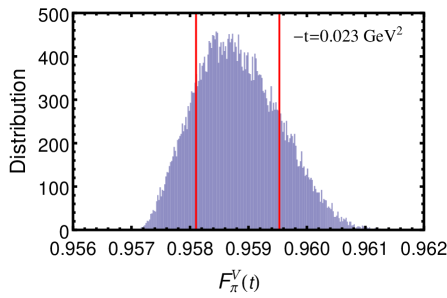
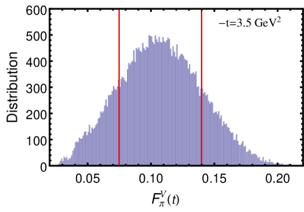
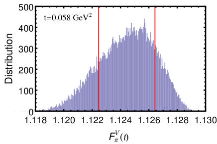
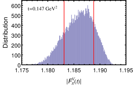
Figure 1: Statistical distributions of the output values of the form factor at two spacelike points (upper panel) and two timelike points, one below and the other above the unitarity threshold $t_{+}$ (lower panel). In the calculation, we used the Bern phase, the input from the spacelike point $t_{s}=-1.6\,\text{GeV}^{2}$, and the modulus at the timelike point $\sqrt{t_{t}}=0.699\,\text{GeV}$ measured by BABAR [38]. The vertical lines indicate the 68.3% confidence limit (CL) intervals).

In Fig. 1, we present for illustration the distributions of the output values of the form factor at several points of interest (two spacelike points in the upper panel, and two timelike points, one below and the other above the unitarity threshold, in the lower panel). The histograms have been obtained using as input the Bern phase, the value at the spacelike point $t_{s}=-1.6\,\text{GeV}^{2}$, and the modulus at one timelike point measured by BABAR [38]. Similar results have been obtained using as input the Madrid phase and other experimental data. One can see that the distributions are very close to a Gaussian and allow the extraction of the mean value and the standard deviation (defined as the 68.3% confidence limit (CL) intervals) for the values of interest $F_{\pi}^{V}(t)$ or its modulus.

The next step is to take the average of the results obtained with input from various measurements. Since the degrees of correlations between the measurements at different energies are expected to vary from one experiment to another, we perform first the average of the values obtained with input from each experiment. As argued in [74], the most robust average of a set of $n$ measurements $a_{i}$ is the weighted average

$$\bar{a}=\sum_{i=1}^{n}w_{i}a_{i},\quad w_{i}=\frac{1/\delta a_{i}^{2}}{\sum_{j=1}^{n}1/\delta a_{j}^{2}},$$ (12)

where $\delta a_{i}$ is the error of $a_{i}$.

For the best estimation of the error in the case of unknown correlations, the prescription proposed in [74] is to define a function $\chi^{2}(f)$

$$\chi^{2}(f)=\sum_{i,j=1}^{n}(a_{i}-\bar{a})(C(f)^{-1})_{ij}(a_{j}-\bar{a})$$ (13)

in terms of the covariance matrix $C(f)$ with elements

$$C_{ij}=\begin{cases}\delta a_{i}\delta a_{i}&\quad\quad\text{if $i=j$},\\ f\delta a_{i}\delta a_{j}&\quad\quad\text{if $i\neq j$}.\end{cases}\$$ (14)

The parameter $f$ denotes the fraction of the maximum possible correlation: for $f=0$ the measurements are treated as uncorrelated, for $f=1$ as fully (100%) correlated.

If $\chi^{2}(0)<n-1$, the data might indicate the existence of a positive correlation. The prescription proposed in [74] is to increase $f$ until $\chi^{2}(f)=n-1$. With the solution $f$ of this equation, the standard deviation $\sigma(\bar{a})$ of $\bar{a}$ is determined from the variance [74]

$$\sigma^{2}(\bar{a})=\left(\sum_{i,j=1}^{n}(C(f)^{-1})_{ij}\right)^{\!\!-1}.$$ (15)

On the other hand, a value $\chi^{2}(0)>n-1$ is an indication that the individual errors are underestimated. If the ratio $\chi^{2}(0)/(n-1)$ is not very far from 1, the procedure suggested in [74, 73] is to rescale the variance $\sigma^{2}(\bar{a})$ calculated with (15) by the factor $\chi^{2}(0)/(n-1)$.

In our work, this procedure was applied first for combining the results obtained with a definite input phase, a specified input (III) from the spacelike region, and different measurements in the timelike region available from each experiment listed in Table 1. In most cases, a large degree of error correlation between the results obtained with different timelike energies was found, as indicated by values close to 1 of the parameter $f$ derived from data. Then the results obtained with the two phases, Bern and Madrid, were combined in a conservative way by taking the simple average of the central values and of the uncertainties. The same conservative average was used for combining the results obtained with the two spacelike data (III).

The last step was to combine the individual values obtained with measurements by the different experiments listed in Table 1. Again, the error correlation for these values is difficult to assess a priori. Therefore, we have applied the same data-driven procedure described above for finding the correlations. Since, as discussed in [2], the data from $e^{+}e^{-}$-annihilation and $\tau$-decay experiments are consistent in the region $0.65-0.71$ GeV, the results from all the 10 experiments in Table 1 can be combined into a single central value and standard deviation which we quote as the error.

V Results

We have applied the procedure described above for deriving central values and standard deviations for $F_{\pi}^{V}(t)$ in three energy regions: small spacelike momenta $Q^{2}=-t\leq 0.25\,\text{GeV}^{2}$, where measurements are available from NA7 experiment [22], larger spacelike momenta, up to $Q^{2}\leq 8.5\,\text{GeV}^{2}$, and the unphysical timelike region $0<t<t_{+}$ below the unitarity threshold. We have also derived central values and standard deviations for the modulus $|F_{\pi}^{V}(t)|$ in the region above the unitarity threshold, below $\sqrt{t}=0.63\,\text{GeV}$, and have used these results for a new determination of the HVP contribution from energies below $0.63\,\text{GeV}$ to the muon $g-2$. In the following subsections we present the results for each kinematical region, namely small spacelike momenta, large spacelike momenta, unphysical timelike momenta, and timelike momenta on the unitarity cut below 0.63 GeV. The implications of these determinations are also studied in each of these subsections.

V.1 Small spacelike momenta

At small spacelike momenta squared, $Q^{2}\leq 0.25\,\text{GeV}^{2}$, the pion form factor has been measured from $ep$ elastic scattering by the NA7 experiment [22], considered for a long time a landmark experiment. Recently, the ETM collaboration [12] reported the most precise lattice calculations of $F_{\pi}^{V}(-Q^{2})$ for small $Q^{2}$. The comparison with the lattice results has been actually the main motivation for choosing this kinematical region in our study. It turns out that our predictions for the form factor in this region are very precise: the errors, obtained by the procedure described in the previous section, vary from 0.0005 near the origin to 0.003 at the end of the region.

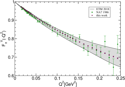
Figure 2: The predictions for the pion form factor in the spacelike region near the origin derived in this work, compared with the experimental results of the NA7 Collaboration [22] and the lattice calculations of the ETM Collaboration [12].

In Fig. 2, we present the values of the form factor calculated in this work at a number of spacelike points below $0.25\,\text{GeV}^{2}$. Also shown are the experimental data from Ref. [22] and the results of the lattice calculation reported in Ref. [12], shown as a band which includes all the uncertainties. One can see that our results are consistent with the lattice values, and are much more precise. It is a challenge for the future lattice calculations to increase the precision to the level reached by the phenomenological determination based on analyticity and unitarity.

It may be noted that our procedure can be extended further as there is no real constraint on the range of values to be probed in this sector, but for practical purposes, our determination has been limited to the same range as in the lattice study and in the NA7 experiment.

V.2 Large spacelike momenta and the onset of perturbative QCD

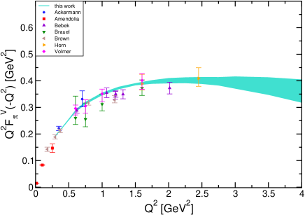
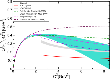
Figure 3: The pion form factor calculated in this work on the spacelike axis, represented as a band which includes the total error. Left panel: comparison with experimental data. Right panel: comparison with perturbative QCD at LO and NLO, and with several nonperturbative models.

It has long been known that in the case of the pion form factor the asymptotic regime described by the dominant term (2) of perturbative QCD sets in quite slowly, due to the complexity of soft, nonperturbative processes in QCD in the intermediate $Q^{2}$ region. Several nonperturbative approaches have been proposed for the study of the pion form factor, including QCD sum rules [75], quark-hadron local duality [76, 77, 78, 79], extended vector meson dominance [80], light-cone sum rules [81, 82, 83], sum rules with nonlocal condensates [84, 85, 86], AdS/QCD models [87, 88], $k_{T}$ factorization method [89], dispersion relations treatment [90], covariant spectator theory [91], and Dyson-Schwinger equation framework [92]. In particular, the onset of the asymptotic regime in the presence of Sudakov corrections [93] and large $N_{c}$ Regge approaches [94] is expected to be quite slow. Constructing a fully valid model to describe the form factor at intermediate energies in fundamental QCD still remains a major theoretical challenge.

Measurements of the spacelike form factor for spacelike momenta are reported in Refs. [23, 24, 25, 26, 27, 28, 29, 30, 31, 32], the most precise being the recent results of the JLab collaboration [31, 32] quoted in Eq. (III). The lack of precise experimental data in the higher $Q^{2}$ region is a major obstacle to confirm or discard the theoretical models available. The calculation presented in this work provides an alternative way for testing the onset of the asymptotic QCD regime and the validity of various theoretical models proposed for intermediate energies.

In the left panel of Fig. 3, the predictions of this work for $Q^{2}<4\,\text{GeV}^{2}$, represented as a cyan band which includes the full error, are compared with some of the experimental data. We recall that in our calculation the only input from the spacelike axis consists of the points given in Eq. (III), denoted as Horn in Fig. 3. The increased precision of our determinations is due to the timelike information. One can see that, except for a few points, the experimental measurements are in general agreement with our determinations.

At higher spacelike momenta, the precision of our predictions starts to diminish, since the extrapolation is more sensitive to the values of the form factor at intermediate timelike energies, for which no precise information is available. To account for this, we have adopted the conservative, weaker condition (6). Up to $Q^{2}$ around $8\,\text{GeV}^{2}$, the precision nevertheless is acceptable, allowing us to probe the onset of the asymptotic regime predicted by factorization and perturbative QCD. In the right panel of Fig. 3, we compare our predictions shown in cyan band with perturbative QCD at LO and NLO, and with some theoretical models. The gray band corresponds to the NLO result obtained by varying the renormalization scale in suitable range following [21]

At first sight we note that perturbative QCD at LO can not reliably describe the form factor at $Q^{2}\leq 7$ GeV². Though the description improves at NLO it is still unreliable for $Q^{2}\leq 5.5$ GeV². We limit ourselves only to these conservative statements, since precisely at the energies where the NLO and our predictions start to become compatible, our procedure meets its natural limitations. This can be seen in the fact that our band hits the $x$-axis in right panel of Fig. 3, while there are strong arguments (cf. for instance Ref. [71]) that this form factor cannot have zeros on the spacelike axis. Therefore, we refrain from making definite statements for higher $Q^{2}$, in view of the fact that this is the region where our method lacks the precision that it has in the other three regimes considered in this work.

As we discussed above, there are many theoretical models in the literature for addressing the properties of the form factors in this region. For illustration, we have considered the predictions from four of these as typical examples. For instance, the theoretical models proposed in [78, 82] appear to be consistent with the phenomenological band, while the predictions of [88, 94] appear to be too high.

We note finally that the results derived in this work are consistent with those derived in our previous work [67], being more precise, since we now included information on the modulus of the form factor on the timelike axis and used extensive Monte Carlo simulations for the error analysis.

V.3 Unphysical timelike region

No experimental information or QCD lattice calculations are available for the pion form factor in the unphysical timelike region between the origin and the unitarity threshold $t_{+}$. For this region our method allows to make very precise predictions. In Table 2, we list the central values and the errors on $F_{\pi}^{V}(t)$ at several unphysical timelike points. This region cannot be accessed by experiment, but it can be by the lattice, in principle, so our results can be viewed as a benchmark for lattice predictions in the future.

$\sqrt{t}$ GeV	$F_{\pi}^{V}(t)$
0.140	$1.037\pm 0.001$
0.197	$1.078\pm 0.001$
$0.242$	$1.124\pm 0.001$
$0.279$	$1.176\pm 0.002$

Table 2: Central values and errors on $F_{\pi}^{V}(t)$ in the timelike region below the unitarity threshold $\sqrt{t_{+}}=2m_{\pi}$.

In this region the predictions of chiral perturbation theory are expected to be most accurate. The precise determinations in table 2 can be used to determine the curvature $c$ and higher shape parameter $d$ of the Taylor expansion $F^{V}_{\pi}(t)=1+\langle r_{\pi}^{2}\rangle t/6+ct^{2}+dt^{3}+\mathcal{O}(t^{4})$.

V.4 Low energies above the unitarity threshold and the contribution to muon $g-2$

As mentioned in the Introduction, above the unitarity threshold, where the form factor is a complex function, its modulus is extracted from the cross section of the $e^{+}e^{-}\to\pi^{+}\pi^{-}$ process, or, using isospin symmetry, from the hadronic decay of the $\tau$ lepton. The $\tau$ decay has been for a long time the most precise source of information, in spite of the nontrivial corrections that are required to convert the measured spectral functions into genuine values of $|F_{\pi}^{V}(t)|$. However, the accuracy of the $e^{+}e^{-}$ experiments improved gradually, the extraction of the modulus being based at present almost exclusively on them.

At low energies, the modulus of the form factor is poorly known, due to the difficulties of the experimental measurements in this region: only two experiments, BABAR [38] and KLOE [40, 41, 42] reported data at low energies, and unfortunately they are not consistent among them. Our method allows a precise determination of $|F_{\pi}^{V}(t)|$ at low energies. In Fig. 4 we present our results, together with the experimental values of BABAR [38] and KLOE [41, 42]. For convenience, we show the values of the modulus squared, which enter directly into the calculation of the two-pion contribution to the muon magnetic anomaly. One can see that our predictions are much more precise than the available experimental results, especially at energies below 0.5 GeV.

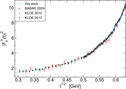
Figure 4: Our predictions for the modulus squared of the pion form factor on the cut below 0.63 GeV, compared with BABAR and KLOE experimental data.

For completeness, we list in Table 3 the central values and the uncertainties of the modulus squared of the form factor at several energies below $0.63\,\text{GeV}$.

$\sqrt{t}$ GeV	$|F_{\pi}^{V}(t)|^{2}$	$\sqrt{t}$ GeV	$|F_{\pi}^{V}(t)|^{2}$
0.281	$1.389\pm 0.004$	$0.437$	$2.485\pm 0.014$
0.283	$1.397\pm 0.004$	$0.455$	$2.712\pm 0.016$
0.285	$1.405\pm 0.004$	$0.472$	$2.978\pm 0.019$
0.291	$1.431\pm 0.004$	$0.490$	$3.291\pm 0.022$
0.297	$1.456\pm 0.004$	$0.507$	$3.664\pm 0.025$
0.314	$1.536\pm 0.005$	$0.525$	$4.111\pm 0.028$
0.332	$1.626\pm 0.006$	$0.542$	$4.653\pm 0.031$
0.349	$1.728\pm 0.007$	$0.560$	$5.318\pm 0.034$
0.367	$1.842\pm 0.008$	$0.577$	$6.144\pm 0.036$
0.384	$1.972\pm 0.009$	$0.595$	$7.174\pm 0.031$
0.402	$2.120\pm 0.011$	$0.612$	$8.498\pm 0.028$
0.419	$2.290\pm 0.012$	$0.630$	$10.177\pm 0.005$

Table 3: Central values and errors on $|F_{\pi}^{V}(t)|^{2}$ in the range from two-pion threshold to 0.63 GeV.

We shall use now these results for making a new determination of the low-energy pion-pion contribution to the muon anomaly. The leading order (LO) two-pion contribution to $a_{\mu}$ from energies below $\sqrt{t_{up}}$, which does not contain the vacuum polarization but includes one-photon final-state radiation (FSR), is expressed in terms of $F_{\pi}^{V}(t)$ as

$$a_{\mu}^{\pi\pi}|_{\leq\sqrt{t_{up}}}=\frac{\alpha^{2}m_{\mu}^{2}}{12\pi^{2}}\int_{t_{+}}^{t_{\text{up}}}\frac{dt}{t}K(t)\ \beta^{3}_{\pi}(t)\ F_{\rm FSR}(t)\ |F_{\pi}^{V}(t)|^{2}.$$ (16)

In this relation, $\beta_{\pi}^{3}(t)=(1-4m_{\pi}/t)^{3/2}$ is the two-pion phase space relevant for $e^{+}e^{-}\to\pi^{+}\pi^{-}$ annihilation,

$$K(t)=\int_{0}^{1}du(1-u)u^{2}(t-u+m_{\mu}^{2}u^{2})^{-1}$$ (17)

is the QED kernel function [95], which exhibits a drastic increase at low $t$, and

$$F_{\rm FSR}(t)=\left(1+\frac{\alpha}{\pi}\,\eta_{\pi}(t)\right)$$ (18)

is the FSR correction, calculated in scalar QED [96, 97].

Using the central values of $|F_{\pi}^{V}(t)|^{2}$ given in Table 3, the integral (16) gives $(132.97\pm 0.07)\times 10^{-10}$, where we quoted an uncertainty due to the method of integration. In order to estimate the statistical error $\sigma_{a_{\mu}}$ of this result, we shall apply the standard error propagation, expressed in our case as

$$\sigma_{a_{\mu}}=\left[\int_{t_{+}}^{t_{\text{up}}}\int_{t_{+}}^{t_{\text{up}}}dtdt^{\prime}\ {\rm Cov}(t,t^{\prime})\ W(t)W(t^{\prime})\right]^{1/2},$$ (19)

where

$$W(t)=\frac{\alpha^{2}m_{\mu}^{2}}{12\pi^{2}}\ \frac{K(t)}{t}\ \beta^{3}_{\pi}(t)\ F_{\rm FSR}(t),$$ (20)

and ${\rm Cov}(t,t^{\prime})$ is the covariance matrix describing the correlation of the errors on $|F_{\pi}^{V}|^{2}$ at two points $t$ and $t^{\prime}$. For a most conservative estimate, we assume fully correlated errors, which means that we take

$${\rm Cov}(t,t^{\prime})=\sigma(t)\sigma(t^{\prime}),$$ (21)

where $\sigma(t)$ is the error on $|F_{\pi}^{V}(t)|^{2}$, determined by the procedure described in Sec. IV. Then the integral (19) gives an error of $0.69\times 10^{-10}$. Adding to this the integration error quoted above, we finally obtain

$$a_{\mu}^{\pi\pi}|_{\leq 0.63\,\text{GeV}}=(132.97\pm 0.70)\times 10^{-10}.$$ (22)

For further comparison, we quote also the result obtained using the timelike input on the modulus in the range (0.65-0.71) GeV only from the $e^{+}e^{-}$ experiments:

$$a_{\mu}^{\pi\pi}|_{\leq 0.63\,\text{GeV}}=(132.91\pm 0.76)\times 10^{-10}.$$ (23)

The values (22) and (23) are fully consistent with our previous results $(133.26\pm 0.72)\times 10^{-10}$ and $(133.02\pm 0.77)\times 10^{-10}$, respectively, obtained in [2] for the same quantities with a slightly different method. The difference stems from the fact that in Ref. [2] we generated the statistical distribution of the integral (16) directly from Monte Carlo simulations, without deriving the modulus squared of the form factor at each energy below 0.63 GeV.

We quote also the result $a_{\mu}^{\pi\pi}|_{\leq 0.63\,\text{GeV}}=132.5(1.1)\times 10^{-10}$ of the recent analysis [64], which exploits analyticity and unitarity by using an extended Omnès representation of the form factor in a global fit of the phenomenological data on $e^{+}e^{-}\to\pi^{+}\pi^{-}$ from energies below 1 GeV and the NA7 experiment. We note also that the direct integration of the interpolation of the $e^{+}e^{-}$ data below 0.63 GeV, proposed in [61], gives $a_{\mu}^{\pi\pi}|_{\leq 0.63\,\text{GeV}}=(131.12\pm 1.03)\times 10^{-10}$.

It may be noted that the explicit values listed in Table 3 for this region allow an evaluation of the dipion contribution to the muon anomaly in any interval of interest.

VI Discussion and Conclusions

In the present work we have obtained high-precision predictions for the pion electromagnetic form factor in several kinematical regions of interest. We have used a method based on analyticity and unitarity, which does not involve standard dispersion relations or specific parametrizations. The input, summarized in Sec. II, consists of the phase of the form factor on a part of the unitarity cut and a conservative integral condition on the modulus squared on the remaining part. The experimental values at some discrete points on the timelike and the spacelike axes are also included.

Using the solution of a functional extremal problem formulated in Sec. II and discussed in the Appendix, we have derived optimal upper and lower bounds on the values of the form factor (or its modulus) in the regions of interest, which are expressed only in terms of the adopted input and involve no model-dependent assumptions. A key element of our method is the determination of the central values and the errors from statistical distributions obtained from a large set of pseudo-data, and the conservative combination of the results from various experiments using data-driven error correlations. We emphasize that, since we do not use a specific parametrization for the form factor and the analytic bounds do not involve model-dependent assumptions, there are no additional systematic errors in our approach. Thus, the Monte Carlo simulations described in Sec. IV give the full errors of our predictions for the form factor.

We mention that the same technique has been applied in [1] for a precise extraction of the pion electromagnetic charge radius, and in [2] for a direct calculation of the two-pion low-energy contribution to muon $g-2$.

The high-precision determinations of the form factor (or its modulus) in several significant kinematical regions are presented in Sec. V. In particular, on the spacelike axis at low $Q^{2}$ our results are much more precise than the recent lattice calculations [12], and at larger $Q^{2}$ we confirm our previous conclusion [67] that the asymptotic regime of perturbative QCD is away from the region $Q^{2}\leq 7\,\text{GeV}^{2}$.

On the timelike axis, we derived high-precision values of the modulus squared of the form factor on the unitarity cut below $0.63\,\text{GeV}$, shown in Fig. 4 and Table 3. Our predictions are much more precise than the experimental values available in this region from BABAR and KLOE experiments, especially below 0.5 GeV. Also, in Sec. V, the determinations we provide in the unphysical timelike region could serve as a benchmark for theoretical probes in this region.

From the precise values given in Table 3, we have performed a new determination of the two-pion contribution from low energies to the muon $g-2$. Our results for $a_{\mu}^{\pi\pi}|_{\leq 0.63\,\text{GeV}}$ are given in Eqs. (22) and (23), where the first uses the input from both $e^{+}e^{-}$ and $\tau$ experiments, and the second only from $e^{+}e^{-}$ experiments. These results are consistent with the values derived in our previous work [2], where the technique of rigorous analytic bounds and Monte Carlo simulations has been applied in a slightly different way, by deriving a statistical distribution directly for the quantity $a_{\mu}^{\pi\pi}|_{\leq 0.63\,\text{GeV}}$.

As seen from the values quoted at the end of the previous section, our results are consistent with the prediction of the recent analysis [64] based on analyticity and unitarity, while the result obtained from the direct integration of the data [61] is slightly lower. We emphasize that we do not use as input experimental data from energies below 0.63 GeV or from NA7 experiment. Thus, our prediction for $a_{\mu}^{\pi\pi}|_{\leq 0.63\,\text{GeV}}$ is to a certain extent complementary to the determination of the analysis performed in [64], which exploits analyticity and unitarity in a different way and uses as input low-energy data.

This work represents the state of the art in an important low-energy sector of the Standard Model, which is going to be tested at the upcoming Fermilab experiment E969. In contrast to our prior publications [1, 2], which were focused on the determination of a single number, here we have obtained an extensive tabulation of the values of the electromagnetic form factor in several significant kinematical regions. Using these determinations, the value of the dipion contribution to the muon anomaly remains consistent with the value reported earlier, proving the robustness of the approach.

The present work combines strong theoretical inputs with modern Monte Carlo methods along with high precision experimental information and phase shift information in regions where experiments are in agreement to shed light on regions where either experiments do not have sufficient precision or where there are significant disagreements, or regions which are not directly accessible by experiment. It also offers a test to theoretical predictions based on very different approaches to strong interaction phenomenology.

Acknowledgments

We would like to thank Urs Wenger for useful correspondence. B.A. acknowledges support from the MSIL Chair of the Division of Physical and Mathematical Sciences, Indian Institute of Science. I.C. acknowledges support from the Ministry of Research and Innovation of Romania, Contract No. PN 18090101/2018. D.D. is supported by the DST, Government of India, under INSPIRE Fellowship (No. DST/INSPIRE/04/2016/002620).

Appendix A Solution of the extremal problem

Using the approach proposed in [65], the extremal problem formulated at the end of Sec. II can be reduced to a standard analytic interpolation problem [98] (also known as a Meiman problem [99]). We review in what follows the main steps of the proof. As discussed in Sec. III, we first remove from the form factor the isospin-violating correction $F_{\omega}(t)$, so in what follows we shall consider the function $F(t)$ defined in (4). The next step is to introduce a function $h(t)$ by writing

$$F(t)={\cal{O}}(t)h(t),$$ (24)

where ${\cal{O}}(t)$ is the Omnès function defined as

$${\cal{O}}(t)=\exp\left(\displaystyle\frac{t}{\pi}\int^{\infty}_{t_{+}}dt^{\prime}\displaystyle\frac{\delta(t^{\prime})}{t^{\prime}(t^{\prime}-t)}\right).$$ (25)

In this relation, $\delta(t)$ is equal to $\delta_{1}^{1}(t)$ at $t\leq t_{\text{in}}$ and is an arbitrary smooth (Lipschitz continuous) function above $t_{\text{in}}$, which approaches asymptotically $\pi$.

From the Fermi-Watson theorem (5), it follows that $h(t)$ is real on the real axis below $t_{\text{in}}$, since the phase of $F(t)$ is exactly compensated by the phase of ${\cal{O}}(t)$. Taking into account the fact that $h(t)$ satisfies the Schwarz reflection property, this implies that it is holomorphic on the real axis below $t_{\text{in}}$, having a branch cut only for $t\geq t_{\text{in}}$.

In terms of $h(t)$, the equality (6) can be written as

$$\frac{1}{\pi}\int_{t_{\text{in}}}^{\infty}dt\,\rho(t)|{\cal{O}}(t)|^{2}|h(t)|^{2}\leq I.$$ (26)

This relation can be written in a canonical form if we perform the conformal transformation,

$$\tilde{z}(t)=\frac{\sqrt{t_{\text{in}}}-\sqrt{t_{\text{in}}-t}}{\sqrt{t_{\text{in}}}+\sqrt{t_{\text{in}}-t}},$$ (27)

and express the factors multiplying $|h(t)|^{2}$ in terms of an outer function, i.e. a function analytic and without zeros in the unit disk $|z|<1$. In practice, it is convenient to construct it as a product of two outer functions [65, 66]: the first one, denoted as $w(z)$, has the modulus equal to $\sqrt{\rho(t)\,|{\rm d}t/{\rm d}\tilde{z}(t)|}$. For the choice $\rho(t)=1/t$, it is given by the simple expression

$$w(z)=\sqrt{\frac{1-z}{1+z}}.$$ (28)

The second outer function, denoted as $\omega(z)$, has the modulus equal to $|{\cal{O}}(t)|$, and can be calculated by the integral representation

$$\omega(z)=\exp\left(\displaystyle\frac{\sqrt{t_{\text{in}}-\tilde{t}(z)}}{\pi}\int^{\infty}_{t_{\text{in}}}\displaystyle\frac{\ln|{\cal{O}}(t^{\prime})|\,{\rm d}t^{\prime}}{\sqrt{t^{\prime}-t_{\text{in}}}(t^{\prime}-\tilde{t}(z))}\right).$$ (29)

If we define the function $g(z)$ by

$$g(z)=w(z)\,\omega(z)\,h(\tilde{t}(z)),$$ (30)

where $\tilde{t}(z)$ is the inverse of $z=\tilde{z}(t)$ defined in Eq.(27), the condition (26) can be written with no loss of information as

$$\frac{1}{2\pi}\int^{2\pi}_{0}{\rm d}\theta|g(\zeta)|^{2}\leq I,\qquad\zeta=e^{i\theta}.$$ (31)

This condition leads to rigorous correlations among the values of the analytic function $g(z)$ and its derivatives at points inside the holomorphy domain, $|z|<1$ (for a proof and earlier references see Ref. [66]) In particular, in our case this amounts to the positivity condition

$${\cal D}\geq 0$$ (32)

of the determinant ${\cal D}$ defined as

$${\cal D}=\left|\begin{array}[]{c c c c c c}I-g(0)^{2}&\xi_{1}&\xi_{2}&\xi_{3}\\ \xi_{1}&\displaystyle\frac{z^{2}_{1}}{1-z^{2}_{1}}&\displaystyle\frac{z_{1}z_{2}}{1-z_{1}z_{2}}&\displaystyle\frac{z_{1}z_{3}}{1-z_{1}z_{3}}\\ \xi_{2}&\displaystyle\frac{z_{1}z_{2}}{1-z_{1}z_{2}}&\displaystyle\frac{z_{2}^{2}}{1-z_{2}^{2}}&\displaystyle\frac{z_{2}z_{3}}{1-z_{2}z_{3}}\\ \xi_{3}&\displaystyle\frac{z_{1}z_{3}}{1-z_{1}z_{3}}&\displaystyle\frac{z_{2}z_{3}}{1-z_{2}z_{3}}&\displaystyle\frac{z_{3}^{2}}{1-z_{3}^{2}}\\ \end{array}\right|,$$ (33)

where the real values $z_{n}\in(-1,1)$ are defined as

$$z_{n}=\tilde{z}(t_{n}),$$ (34)

in terms of the two points $t_{1}=t_{s}$ and $t_{2}=t_{t}$ used as input and the value $t_{3}$ where we want to calculate bounds on the form factor, and

$$\xi_{n}=g(z_{n})-g(0),\quad 1\leq n\leq 3.$$ (35)

The inequality (32) defines an allowed domain for the real values $g(z_{n})$. For $n=1$ and $n=3$ with $t<t_{+}$, we have from Eqs. (24) and (30)

$$g(z_{n})=w(z_{n})\,\omega(z_{n})\,F(t_{n})/{\cal{O}}(t_{n}),$$ (36)

while for $n=2$ and $n=3$ with $t>t_{+}$

$$g(z_{n})=w(z_{n})\,\omega(z_{n})\,|F(t_{n})|/|{\cal{O}}(t_{n})|,$$ (37)

where the modulus $|{\cal{O}}(t)|$ of the Omnès function is obtained from (25) by the principal value (PV) Cauchy integral

$$|{\cal{O}}(t)|=\exp\left(\frac{t}{\pi}\text{\rm PV}\int^{\infty}_{t_{+}}dt^{\prime}\displaystyle\frac{\delta(t^{\prime})}{t^{\prime}(t^{\prime}-t)}\right).$$ (38)

One can show that for each specific input, the determinant (33) is a concave quadratic function of the unknown value $F(t_{3})$ for $t_{3}<t_{+}$, or the modulus $|F(t_{3})|$ for $t_{3}>t_{+}$, so the inequality (32) can be written as

$$Ax^{2}+2Bx+C\geq 0,\quad A\leq 0,$$ (39)

where $x=F(t_{3})$ or $x=|F(t_{3})|$. This inequality leads to a definite allowed range for $x$ if $B^{2}-AC\geq 0$ and has no solution if $B^{2}-AC<0$. The latter case occurs when the phenomenological input adopted is inconsistent with analyticity.

From the inequality (39), one can obtain upper and lower bounds on $F(t_{3})$ (or $|F(t_{3})|$), expressed in terms of the adopted input. Finally, the isospin correction is applied back according to (4), for obtaining the desired bounds on the form factor $F_{\pi}^{V}(t)$.

One can prove [65, 66], that the bounds are optimal and their values do not depend on the unknown phase of the form factor above the inelastic threshold $t_{\text{in}}$ (the dependence of the Omnès function (25) on the arbitrary phase $\delta(t)$ for $t>t_{\text{in}}$ is compensated exactly by the corresponding dependence of the outer function (29)). Furthermore, for a fixed weight $\rho(t)$ in (6), the bounds become stronger/weaker when the value of the value of $I$ is decreased or increased, respectively. These properties make the formalism model independent and robust against the uncertainties from the high energy region.

References

- [1] B. Ananthanarayan, I. Caprini and D. Das, Electromagnetic charge radius of the pion at high precision, Phys. Rev. Lett. 119, 132002 (2017) [arXiv:1706.04020 [hep-ph]].
- [2] B. Ananthanarayan, I. Caprini, D. Das and I. Sentitemsu Imsong, Precise determination of the low-energy hadronic contribution to the muon from analyticity and unitarity: An improved analysis, Phys. Rev. D 93, 116007 (2016), [arXiv:1605.00202 [hep-ph]].
- [3] S. Weinberg, Phenomenological lagrangians, Physica A 96, 327 (1979).
- [4] J. Gasser and H. Leutwyler, Chiral perturbation theory to one loop, Annals Phys. 158, 142 (1984).
- [5] J. Gasser and H. Leutwyler, Chiral perturbation theory: expansions in the mass of the strange quark, Nucl. Phys. B 250, 465 (1985).
- [6] J. Gasser and H. Leutwyler, Low-energy expansion of meson form-factors, Nucl. Phys. B 250 (1985) 517.
- [7] J. Gasser and U.G. Meissner, Chiral expansion of pion form-factors beyond one loop, Nucl. Phys. B 357, 90 (1991) .
- [8] G. Colangelo, M. Finkemeier and R. Urech, Tau decays and chiral perturbation theory, Phys. Rev. D 54, 4403 (1996) [arXiv:hep-ph/9604279].
- [9] J. Bijnens, G. Colangelo and P. Talavera, The vector and scalar form factors of the pion to two loops, JHEP 9805, 014 (1998) [arXiv:hep-ph/9805389].
- [10] J.Bijnens and P. Talavera, Pion and kaon electromagnetic form factors, JHEP 0203, 046 (2002) [arXiv:hep-ph/0203049].
- [11] J. Bijnens, G. Colangelo and P. Talavera, The vector and scalar form-factors of the pion to two loops, JHEP 9805, 014 (1998), [hep-ph/9805389].
- [12] C. Alexandrou et al. [ETM Collaboration], Pion vector form factor from lattice QCD at the physical point, Phys. Rev. D 97, 014508 (2018), [arXiv:1710.10401 [hep-lat]].
- [13] S. Aoki et al., Review of lattice results concerning low-energy particle physics, Eur.Phys.J. C77, 112 (2017), [arXiv:1607.00299 [hep-lat]].
- [14] G. P. Lepage and S. J. Brodsky, Exclusive processes in quantum chromodynamics: Evolution equations for hadronic wave functions and the form factors of mesons, Phys. Lett. B 87, 359 (1979).
- [15] G. R. Farrar and D. R. Jackson, The pion form factor, Phys. Rev. Lett. 43, 246 (1979).
- [16] G. P. Lepage and S. J. Brodsky, Exclusive processes in perturbative Quantum Chromodynamics, Phys. Rev. D 22, 2157 (1980).
- [17] A. V. Efremov and A. V. Radyushkin, Factorization and asymptotical behavior of pion form-factor in QCD, Phys. Lett. B 94, 245 (1980).
- [18] V. L. Chernyak and A. R. Zhitnitsky, Asymptotic behavior of hadron form-factors in quark model. (In Russian), JETP Lett. 25, 510 (1977) [Pisma Zh. Eksp. Teor. Fiz. 25, 544 (1977)].
- [19] V. L. Chernyak and A. R. Zhitnitsky, Asymptotic Behavior of Exclusive Processes in QCD, Phys. Rept. 112, 173 (1984).
- [20] B. Melic, B. Nizic and K. Passek, Complete next-to-leading order perturbative QCD prediction for the pion form-factor, Phys. Rev. D 60, 074004 (1999) [arXiv:hep-ph/9802204].
- [21] B. Melic, B. Nizic and K. Passek, On the PQCD prediction for the pion form-factor, hep-ph/9908510.
- [22] S.R. Amendolia et al. [NA7 Collaboration], A measurement of the space - like pion electromagnetic form-factor, Nucl. Phys. B 277, 168 (1986).
- [23] C.N. Brown et al., Coincidence electroproduction of charged pions and the pion form-factor, Phys. Rev. D 8, 92 (1973).
- [24] C.J. Bebek et al., Further measurements of forward-charged-pion electroproduction at large , Phys. Rev. D 9, 1229 (1974).
- [25] C. J. Bebek et al., Measurement of the pion form-factor up to = 4-GeV2, Phys. Rev. D 13 (1976) 25.
- [26] H. Ackermann et al., Determination of the longitudinal and the transverse part in electroproduction, Nucl. Phys. B 137, 294 (1978).
- [27] C.J. Bebek et al., Electroproduction of single pions at low epsilon and a measurement of the pion form-factor up to , Phys. Rev. D 17, 1693 (1978).
- [28] P. Brauel et al., Electroproduction of And final states above the resonance region, Z. Phys. C 3, 101 (1979).
- [29] J. Volmer et al. [The Jefferson Lab Collaboration], New results for the charged pion electromagnetic form-factor, Phys. Rev. Lett. 86, 1713 (2001), [arXiv:nucl-ex/0010009].
- [30] V. Tadevosyan et al. [Jefferson Lab Collaboration], Determination of the pion charge form factor for Q2=0.60-1.60 GeV2, Phys. Rev. C 75, 055205 (2007), [arXiv:nucl-ex/0607007].
- [31] T. Horn et al. [Jefferson Lab Collaboration], Determination of the Charged Pion Form Factor at and 2.45 (GeV/c)2, Phys. Rev. Lett. 97, 192001 (2006), [arXiv:nucl-ex/0607005].
- [32] G.M. Huber et al. [Jefferson Lab Collaboration], Charged pion form factor between and 2.45 GeV2. II. Determination of, and results for, the pion form factor, Phys. Rev. C 78, 045203 (2008), [arXiv:0809.3052 [nucl-ex]].
- [33] G.M. Huber et al. [Jefferson Lab Collaboration], Separated response function ratios in exclusive, forward electroproduction, Phys. Rev. Lett. 112, 182501 (2014), [arXiv:1404.3985 [nucl-ex]].
- [34] R. R. Akhmetshin et al. [CMD-2 Collaboration], High-statistics measurement of the pion form factor in the rho-meson energy range with the CMD-2 detector, Phys. Lett. B 648, 28 (2007), [hep-ex/0610021].
- [35] R. R. Akhmetshin et al. [CMD-2 Collaboration], Reanalysis of hadronic cross-section measurements at CMD-2, Phys. Lett. B 578, 285 (2004), [hep-ex/0308008].
- [36] V. M. Aulchenko et al., Measurement of the cross section with the CMD-2 detector in the 370 - 520-MeV c.m. energy range, JETP Lett. 84, 413 (2006) [Pisma Zh. Eksp. Teor. Fiz. 84, 491 (2006)], [hep-ex/0610016].
- [37] M. N. Achasov et al., Update of the cross-section measured by SND detector in the energy region 400-MeV 1000-MeV, J. Exp. Theor. Phys. 103, 380 (2006) [Zh. Eksp. Teor. Fiz. 130, 437 (2006)], [hep-ex/0605013].
- [38] B. Aubert et al. [BaBar Collaboration], Precise measurement of the Cross Section with the initial state radiation method at BABAR, Phys. Rev. Lett. 103, 231801 (2009), [arXiv:0908.3589 [hep-ex]].
- [39] J. P. Lees et al. [BaBar Collaboration], Precise measurement of the cross section with the initial state radiation method at BABAR, Phys. Rev. D 86, 032013 (2012), [arXiv:1205.2228 [hep-ex]].
- [40] F. Ambrosino et al. [KLOE Collaboration], Measurement of and the dipion contribution to the muon anomaly with the KLOE detector, Phys. Lett. B 670, 285 (2009), [arXiv:0809.3950 [hep-ex]].
- [41] F. Ambrosino et al. [KLOE Collaboration], Measurement of from threshold to 0.85 GeV2 using initial state radiation with the KLOE detector, Phys. Lett. B 700, 102 (2011), [arXiv:1006.5313 [hep-ex]].
- [42] D. Babusci et al. [KLOE Collaboration], Precision measurement of and determination of the contribution to the muon anomaly with the KLOE detector, Phys. Lett. B 720, 336 (2013), [arXiv:1212.4524 [hep-ex]].
- [43] R. R. Akhmetshin et al., Current status of luminosity measurement with the CMD-3 detector at the VEPP-2000 collider, JINST 9, C09003 (2014).
- [44] V. M. Aulchenko et al. [SND Collaboration], Measurement of the cross section in the center-of-mass energy range 1.22-2.00 GeV with the SND detector at the VEPP-2000 collider, Phys. Rev. D 91, no. 5, 052013 (2015), [arXiv:1412.1971 [hep-ex]].
- [45] G. V. Fedotovich et al., Preliminary results of measurements of hadronic cross sections with the CMD-3 detector at the VEPP-2000 electron-positron collider, Phys. Atom. Nucl. 78, no. 5, 591 (2015) [Yad. Fiz. 78, 635–646 (2015)].
- [46] M. Ablikim et al. [BESIII Collaboration], Measurement of the cross section between 600 and 900 MeV using initial state radiation, Phys. Lett. B 753, 629 (2016), [arXiv:1507.08188 [hep-ex]].
- [47] S. Anderson et al. [CLEO Collaboration], Hadronic structure in the decay , Phys. Rev. D 61, 112002 (2000), [hep-ex/9910046].
- [48] S. Schael et al. [ALEPH Collaboration], Branching ratios and spectral functions of decays: Final ALEPH measurements and physics implications, Phys. Rept. 421, 191 (2005), [hep-ex/0506072].
- [49] M. Davier, A. Höcker, B. Malaescu, C. Z. Yuan and Z. Zhang, Update of the ALEPH non-strange spectral functions from hadronic decays, Eur. Phys. J. C 74, no. 3, 2803 (2014), [arXiv:1312.1501 [hep-ex]].
- [50] K. Ackerstaff et al. [OPAL Collaboration], Measurement of the strong coupling constant alpha(s) and the vector and axial vector spectral functions in hadronic tau decays, Eur. Phys. J. C 7, 571 (1999), [hep-ex/9808019].
- [51] M. Fujikawa et al. [Belle Collaboration], High statistics study of the decay, Phys. Rev. D 78, 072006 (2008), [arXiv:0805.3773 [hep-ex]].
- [52] E. Fermi, Lectures on pions and nucleons, Nuovo Cim. 2S1, 17 (1955) [Riv. Nuovo Cim. 31, 1 (2008)].
- [53] K. M. Watson, Some general relations between the photoproduction and scattering of mesons, Phys. Rev. 95, 228 (1954).
- [54] B. Ananthanarayan, G. Colangelo, J. Gasser and H. Leutwyler, Roy equation analysis of scattering, Phys. Rept. 353, 207 (2001), [hep-ph/0005297].
- [55] I. Caprini, G. Colangelo and H. Leutwyler, Regge analysis of the scattering amplitude, Eur. Phys. J. C 72, 1860 (2012), [arXiv:1111.7160 [hep-ph]].
- [56] R. Garcia-Martin, R. Kaminski, J. R. Pelaez, J. Ruiz de Elvira and F. J. Yndurain, The pion-pion scattering amplitude. IV: Improved analysis with once subtracted Roy-like equations up to 1100 MeV, Phys. Rev. D 83, 074004 (2011), [arXiv:1102.2183 [hep-ph]].
- [57] G. Venanzoni [Muon g-2 Collaboration], The new muon experiment at Fermilab, Nucl. Phys. Proc. Suppl. 225-227, 277 (2012).
- [58] T. Mibe [J-PARC g-2 Collaboration], Measurement of muon g-2 and EDM with an ultra-cold muon beam at J-PARC, Nucl. Phys. Proc. Suppl. 218 (2011) 242.
- [59] G. W. Bennett et al. [Muon g-2 Collaboration], Final report of the muon E821 anomalous magnetic moment measurement at BNL, Phys. Rev. D 73, 072003 (2006), [hep-ex/0602035].
- [60] M. Davier, A. Hoecker, B. Malaescu and Z. Zhang, Reevaluation of the hadronic vacuum polarisation contributions to the Standard Model predictions of the muon and using newest hadronic cross-section data, Eur. Phys. J. C 77, 827 (2017), [arXiv:1706.09436 [hep-ph]].
- [61] A. Keshavarzi, D. Nomura and T. Teubner, Muon and : a new data-based analysis, Phys. Rev. D 97, 114025 (2018), [arXiv:1802.02995 [hep-ph]].
- [62] T. Blum et al. [RBC and UKQCD Collaborations], Calculation of the hadronic vacuum polarization contribution to the muon anomalous magnetic moment, Phys. Rev. Lett. 121, 022003 (2018), [arXiv:1801.07224 [hep-lat]].
- [63] C. Hanhart et al., The branching ratio revisited, Eur. Phys. J. C77, 98 (2017), Erratum: Eur.Phys. J. C78, 450 (2018), [arXiv:1611.09359 [hep-ph]].
- [64] G. Colangelo, M. Hoferichter and P. Stoffer, Two-pion contribution to hadronic vacuum polarization, [arXiv:1810.00007 [hep-ph]].
- [65] I. Caprini, Dispersive and chiral symmetry constraints on the light meson form-factors, Eur. Phys. J. C 13, 471 (2000), [hep-ph/9907227].
- [66] G. Abbas, B. Ananthanarayan, I. Caprini, I. Sentitemsu Imsong and S. Ramanan, Theory of unitarity bounds and low energy form factors, Eur. Phys. J. A 45, 389 (2010), [arXiv:1004.4257 [hep-ph]].
- [67] B. Ananthanarayan, I. Caprini and I. S. Imsong, Spacelike pion form factor from analytic continuation and the onset of perturbative QCD, Phys. Rev. D 85, 096006 (2012), [arXiv:1203.5398 [hep-ph]].
- [68] B. Ananthanarayan, I. Caprini, D. Das and I. S. Imsong, Model independent bounds on the modulus of the pion form factor on the unitarity cut below the threshold, Eur. Phys. J. C 72, 2192 (2012), [arXiv:1209.0379 [hep-ph]].
- [69] B. Ananthanarayan, I. Caprini, D. Das and I. Sentitemsu Imsong, Parametrisation-free determination of the shape parameters for the pion electromagnetic form factor, Eur. Phys. J. C 73, 2520 (2013), [arXiv:1302.6373 [hep-ph]].
- [70] B. Ananthanarayan, I. Caprini, D. Das and I. S. Imsong, Two-pion low-energy contribution to the muon with improved precision from analyticity and unitarity, Phys. Rev. D 89, no. 3, 036007 (2014), [arXiv:1312.5849 [hep-ph]].
- [71] H. Leutwyler, Electromagnetic form factor of the pion, in: Continuous advances in QCD 2002, eds. K. A. Olive, M. A. Shifman, and M. B. Voloshin, World Scientific, Singapore, pp. 23–40, (2003), [arXiv:hep-ph/0212324].
- [72] C. Hanhart, A new parameterization for the pion vector form factor, Phys. Lett. B 715, 170 (2012), [arXiv:1203.6839 [hep-ph]].
- [73] M. Tanabashi et al. [Particle Data Group], Review of Particle Physics, Phys. Rev. D 98 (2018) no.3, 030001.
- [74] M. Schmelling, Averaging correlated data, Phys. Scripta 51, 676 (1995).
- [75] B. L. Ioffe and A. V. Smilga, Pion form-factor at intermediate momentum transfer in QCD, Phys. Lett. 114B, 353 (1982).
- [76] V. A. Nesterenko and A. V. Radyushkin, Sum rules and pion form-factor in QCD, Phys. Lett. 115B, 410(1982).
- [77] A.V. Radyushkin, Quark - hadron duality and intrinsic transverse momentum, Acta Phys. Polon. B 26, 2067 (1995), [hep-ph/9511272].
- [78] A. V. Radyushkin, QCD calculations of pion electromagnetic and transition form-factors, [hep-ph/0106058].
- [79] V. Braguta, W. Lucha and D. Melikhov, Pion form-factor at spacelike momentum transfers from local-duality QCD sum rule, Phys. Lett. B 661, 354 (2008), [arXiv:0710.5461 [hep-ph]].
- [80] C.A. Dominguez, Electromagnetic form-factor of the pion: vector mesons or quarks?, Phys. Rev. D 25, 3084 (1982).
- [81] V.M. Braun and I.E. Halperin, Soft contribution to the pion form-factor from light cone QCD sum rules, Phys. Lett. B 328, 457 (1994), [hep-ph/9402270].
- [82] V.M. Braun, A. Khodjamirian and M. Maul, Pion form-factor in QCD at intermediate momentum transfers, Phys. Rev. D 61, 073004 (2000) [arXiv:hep-ph/9907495].
- [83] J. Bijnens and A. Khodjamirian, Exploring light cone sum rules for pion and kaon form-factors, Eur. Phys. J. C 26, 67 (2002), [hep-ph/0206252].
- [84] A.P. Bakulev and A.V. Radyushkin, Nonlocal condensates and QCD sum rules for the pion form-factor, Phys. Lett. B 271, 223 (1991).
- [85] A.P. Bakulev, K. Passek-Kumericki, W. Schroers and N.G. Stefanis, Pion form factor in QCD: From nonlocal condensates to NLO analytic perturbation theory, Phys. Rev. D 70, 033014 (2004) [Erratum-ibid. D 70, 079906 (2004)], [arXiv:hep-ph/0405062].
- [86] A.P. Bakulev, A.V. Pimikov and N.G. Stefanis, QCD sum rules with nonlocal condensates and the spacelike pion form factor, Phys. Rev. D 79, 093010 (2009), [arXiv:0904.2304 [hep-ph]].
- [87] H. R. Grigoryan and A. V. Radyushkin, Pion form-factor in chiral limit of hard-wall AdS/QCD model, Phys. Rev. D 76, 115007 (2007), [arXiv:0709.0500 [hep-ph]].
- [88] S. J. Brodsky and G. F. de Teramond, Light-front dynamics and AdS/QCD correspondence: the pion form factor in the space- and timelike regions, Phys. Rev. D 77, 056007 (2008), [arXiv:0707.3859 [hep-ph]].
- [89] S. Cheng and Z. J. Xiao, Time-like pion electromagnetic form factors in factorization with the next-to-leading-order twist-3 contribution, Phys. Lett. B 749, 1 (2015), [arXiv:1505.02909 [hep-ph]].
- [90] M. Gorchtein, P. Guo and A. P. Szczepaniak, Asymptotic Behavior of Pion Form Factors, arXiv:1106.5252 [hep-ph].
- [91] E. P. Biernat, F. Gross, T. Peña and A. Stadler, Pion electromagnetic form factor in the Covariant Spectator Theory, Phys. Rev. D 89, no. 1, 016006 (2014), [arXiv:1310.7465 [hep-ph]].
- [92] L. Chang, I. C. Cloët, C. D. Roberts, S. M. Schmidt and P. C. Tandy, Pion electromagnetic form factor at spacelike momenta, Phys. Rev. Lett. 111, no. 14, 141802 (2013), [arXiv:1307.0026 [nucl-th]].
- [93] T. Gousset and B. Pire, Timelike form-factors at high-energy, Phys. Rev. D 51, 15 (1995), [hep-ph/9403293].
- [94] E. Ruiz Arriola and W. Broniowski, Pion electromagnetic form factor, perturbative QCD, and large-N(c) Regge models, Phys. Rev. D 78, 034031 (2008), [arXiv:0807.3488 [hep-ph]].
- [95] A. Czarnecki and W. J. Marciano, The muon anomalous magnetic moment: A harbinger for ‘new physics’, Phys. Rev. D 64, 013014 (2001), [hep-ph/0102122].
- [96] H. Czyz, A. Grzelinska, J. H. Kuhn and G. Rodrigo, The radiative return at and -factories: FSR for muon pair production at next-to-leading order, Eur. Phys. J. C 39, 411 (2005), [hep-ph/0404078].
- [97] Y. M. Bystritskiy, E. A. Kuraev, G. V. Fedotovich and F. V. Ignatov, The cross sections of the muons and charged pions pairs production at electron-positron annihilation near the threshold, Phys. Rev. D 72, 114019 (2005), [hep-ph/0505236].
- [98] P. Duren, Theory of Spaces, Academic Press, New York, 1970.
- [99] N.N. Meiman, Analytic expressions for upper limits of coupling constants in quantum field theory, Sov. Phys. JETP 17, 830 (1963).