Dynamics of a quantum oscillator coupled with a three-level $\Lambda-$ type emitter

Abstract

We investigate the quantum dynamics of a quantum oscillator coupled with the most upper state of a three-level $\Lambda-$ type system. The two transitions of the three-level emitter, possessing orthogonal dipole moments, are coherently pumped with a single or two electromagnetic field sources, respectively. We have found ranges for flexible lasing or cooling phenomena referring to the quantum oscillator’s degrees of freedom. This is due to asymmetrical decay rates and quantum interference effects leading to population transfer among the relevant dressed states of the emitter’s subsystem with which the quantum oscillator is coupled. As an appropriate system can be considered a nanomechanical resonator coupled with the most excited state of the three-level emitter fixed on it. Alternatively, if the upper state of the $\Lambda-$type system possesses a permanent dipole then it can couple with a cavity electromagnetic field mode which can be in the terahertz domain, for instance. In the latter case, we demonstrate an effective electromagnetic field source of terahertz photons.

I Introduction

Lasing and cooling effects are among the most studied ones due to their enormous potential applications in the micro- or nano-world rew_art1 ; n_las ; d_las ; las_c ; fon_l . Presently, quantum technologies qt ; qt1 ; qt2 require precise tools allowing a complete control of the quantum interaction between light and matter and, of course, the above mentioned phenomena occurring in a wide range of systems. Particularly, certain quantum systems offer additional control mechanisms via externally applied coherent light sources and, therefore, cooling phenomenon was successfully demonstrated in few-level atomic systems eit_theor ; eit_cool ; ek ; plenio1 , for instance. On the other side, various optomechanical systems are intensively investigated recently because of their extreme sensitivity to ultra-weak perturbations rew_art2 ; rew_art3 . Thereby, cooling or lasing in these systems are of fundamental interest as well las_c ; xe ; phon_las ; cool_exp1 ; cool_exp2 . Furthermore, artificially created atomiclike systems such as quantum dots or quantum wells are also suitable for modern applications and exhibit an advantage with respect to engineering of their dipole moments, transition frequencies, etc. qwell ; qdots ; victor . In these circumstances, ground-state cooling of a nanomechanical resonator with a triple quantum dot via quantum interference effects was demonstrated in gxl1 , see also gxl2 ; plenio2 ; plenio3 . Enhanced nanomechanical resonator’s phonon emission via multiple excited quantum dots was demonstrated as well, in Ref. vpm . Moreover, among other applications of these systems or various optoelectronical schemes is the generation of electromagnetic field in the terahertz domain. The importance of the terahertz waves towards sensing, imaging, spectroscopy or data communications is highly recognized thz1 ; thz2 ; thz3 . In this context, quantum systems possessing permanent dipoles were shown to generate terahertz light tera1 ; tera2 ; terra ; tera3 ; tera4 . Additionally, they exhibit bare-state population inversion as well as multiple spectral lines and squeezing mmk ; gagik ; paspalakis .

Thus, there is an increased interest for novel quantum systems exhibiting lasing in a broad parameter range or cooling of micro- or nano-scale devices. From this point of view, here, we investigate a laser pumped $\Lambda-$type three-level system the upper state of which is being coupled with a quantum oscillator described by a quantized single-mode boson field. More specifically, as a quantum oscillator can serve a vibrational mode of a nanomechanical resonator containing the three-level emitter or, respectively, an electromagnetic cavity mode field if the upper state of the three-level sample, embedded in the cavity, possesses a permanent dipole. The frequency of the quantum oscillator is significant smaller than all other frequencies involved to describe the model, however, it is of the order of the generalized Rabi frequency characterizing the laser-pumped three-level qubit. In concordance to the dressed-state picture of the three-level system, we have identified two resonance conditions determining the oscillator’s quantum dynamics, namely, when the quantum oscillator’s frequency is close to the doubled generalized Rabi frequency or just to the generalized Rabi frequency, respectively. Correspondingly, we treat these two situations separately. We have found steady-state lasing or cooling regimes in both situations for the quantum oscillator’s field mode, however, for asymmetrical spontaneous decay rates corresponding to each three-level qubit’s transition. The mechanisms responsible for these effects are completely different for the two situations. In the case when the doubled generalized Rabi frequency is close to the oscillator’s one, the model is somehow similar to a two-level system interacting with a quantized field mode where the spontaneous decay pumps both levels. On the other side, if the oscillator’s frequency lies near resonance with the generalized Rabi frequency, then the sample is close to an equidistant three-level system where the single-mode quantum oscillator interacts with both qubit’s transitions. The latter situation includes single- or two-quanta processes accompanied by quantum interference effects among the involved dressed-states leading to deeper cooling regimes and flexible ranges for lasing effects. This is different from other related schemes based on electromagnetically induced transparency processes gxl1 ; gxl2 ; plenio2 ; plenio3 . In the case the model contains an electromagnetic cavity mode, which describes the quantum oscillator, then its frequency can be in the terahertz domain and, thus, we demonstrate an effective coherent electromagnetic field source of such photons. While lasing or cooling effects are available for two-level systems as well d_las ; las_c ; fon_l , three-level ones may have an advantage in the sense that show improved results for the same parameters involved. This may help when there are only certain accessible parameter ranges. Furthermore, certain realistic novel systems are described by a three-level model. For instance, as a concrete $\Lambda-$type system may be taken a laser-pumped color center emitter embedded on a vibrating membrane where strong coupling strengths can be achieved via vacuum dispersive forces plenio3 . Few coupled quantum dots are appropriate systems too gxl2 ; qpd . Also, as alternative systems can be asymmetrical real or artificial few-level molecules possessing permanent dipoles, $d_{\alpha\alpha}\not=0$ tera1 ; tera2 ; terra ; tera3 ; tera4 ; mmk ; gagik ; paspalakis ; gong ; qw . If $d_{11}\gg\{d_{22},d_{33}\}$, then an electromagnetic resonator mode can couple with the upper state of the $\Lambda-$type system via its permanent dipole.

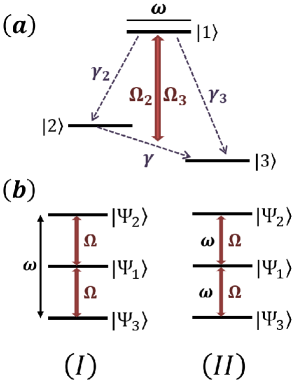
Figure 1: (a) The schematic of the model: A laser pumped three-level $\Lambda-$type system the upper state of which, $|1\rangle$, is coupled with a quantum oscillator mode of frequency $\omega$. The oscillator can be described by a single mode of a nano-mechanical resonator containing the three-level emitter. Alternatively, if the upper state of the three-level system possesses a permanent dipole then it can couple with an electromagnetic cavity mode which can be in the terahertz ranges, for instance. Here, the pumping laser’s frequencies are equal to the average transition frequency of the three-level emitter $(\omega_{12}+\omega_{13})/2$. $\Omega_{2}$ and $\Omega_{3}$ are the corresponding laser-qubit coupling strengths, i.e. the Rabi frequencies, whereas $\gamma^{\prime}s$ are the respective spontaneous decay rates. (b) The semi-classical laser-qubit dressed-state picture where each bare-state level is dynamically split in three dressed-states $\{|\Psi_{2}\rangle,|\Psi_{1}\rangle,|\Psi_{3}\rangle\}$. Resonances occur at: (I) $\omega=2\Omega$ or (II) $\omega=\Omega$, respectively, where $\Omega$ is the generalized Rabi frequency.

The article is organized as follows. In Sec. II we describe the analytical approach and the system of interest, while in Sec. III we analyze the obtained results. The summary is given in Sec. IV.

II Theoretical framework

The Hamiltonian describing a quantum oscillator of frequency $\omega$ coupled with a laser-pumped $\Lambda-$type three-level system, see Fig. 1(a), in a frame rotating at $(\omega_{12}+\omega_{13})/2$, is:

$$H = \hbar\omega b^{\dagger}b+\frac{\hbar\omega_{23}}{2}(S_{22}-S_{33})+\hbar gS_{11}(b+b^{\dagger})$$ (1)

$$- \hbar\sum_{\alpha\in\{2,3\}}\Omega_{\alpha}(S_{1\alpha}+S_{\alpha 1}).$$

We have assumed here that as a pumping electromagnetic field source it can act a single laser of frequency $\omega_{L}$ pumping both arms of the emitter or, respectively, two lasers fields $\{\omega_{L1},\omega_{L2}\}$ each driving separately the two transitions of the $\Lambda-$ type sample possessing orthogonal transition dipoles. Additionally, we have also considered that $\omega_{L1}=\omega_{L2}\equiv(\omega_{12}+\omega_{13})/2$, see Fig. 1(a). Here $\omega_{\alpha\beta}$ are the frequencies of $|\alpha\rangle\leftrightarrow|\beta\rangle$ three-level qubit’s transitions, $\{\alpha,\beta\in 1,2,3\}$. The components entering in the Hamiltonian (1) have the usual meaning, namely, the first and the second terms describe the free energies of the quantum oscillator and the atomic subsystem, respectively, whereas the third one accounts for their mutual interaction via the most upper-state energy level with $g$ being the respective coupling strength. The last term represents the atom-laser interaction and $\{\Omega_{2},\Omega_{3}\}$ are the corresponding Rabi frequencies associated with a particular driven transition. Note that if the upper state of the investigated model contains a permanent dipole then the external coherent light sources interact with it as well. The corresponding Hamiltonian is: $H_{pd}=\hbar S_{11}\sum_{i\in\{2,3\}}G_{i}\cos{(\omega_{Li}t)}$, where $G_{i}=d_{11}E_{i}/\hbar$ with $E_{i}$ being the lasers amplitudes. However, the Hamiltonian $H_{pd}$ can be considered as rapidly oscillating, because $\omega_{Li}\gg G_{i}$, and being further neglected. Thus, the Hamiltonian (1) and the analytical approach developed here allow to treat concomitantly both situations, namely, when either a nanomechanical resonator or an electromagnetic cavity is taken as a quantum oscillator. Finally, the three-level qubit’s operators, $S_{\alpha\beta}=|\alpha\rangle\langle\beta|$, obey the commutation relation $[S_{\alpha\beta},S_{\beta^{\prime}\alpha^{\prime}}]$=$\delta_{\beta\beta^{\prime}}S_{\alpha\alpha^{\prime}}$ - $\delta_{\alpha^{\prime}\alpha}S_{\beta^{\prime}\beta}$ whereas those of the quantum oscillator’s: $[b,b^{\dagger}]=1$ and $[b,b]=[b^{\dagger},b^{\dagger}]=0$, respectively.

In the Born-Markov approximations agarwal_2014 ; gardiner ; wals , the whole quantum dynamics of this complex model can be monitored via the following master equation:

$$\dot{\rho} + \frac{i}{\hbar}[H,\rho]=-\sum_{\alpha\in\{2,3\}}\gamma_{\alpha}[S_{1\alpha},S_{\alpha 1}\rho]-\gamma[S_{23},S_{32}\rho]$$ (2)

$$- \kappa(1+\bar{n})[b^{\dagger},b\rho]-\kappa\bar{n}[b,b^{\dagger}\rho]+H.c..$$

The right-hand side of Eq. (2) describes the emitter’s damping due to spontaneous emission as well as the quantum oscillator’s damping effects with $\bar{n}=1/[\exp{(\hbar\omega/k_{B}T)}-1]$ being the mean oscillator’s quanta number due to the environmental thermostat at temperature $T$. Here $k_{B}$ is the Boltzmann constant, $\gamma$’s are the corresponding decay rates of the three-level qubit, see Fig. 1(a), while $\kappa$ describes the quantum oscillator’s leaking rate, respectively. The physics behind our model can be easier highlighted if we turn to the three-level qubit-laser dressed-state picture given by the transformation:

$$|1\rangle = \sin{\theta}|\Psi_{1}\rangle-\frac{\cos{\theta}}{\sqrt{2}}\bigl{(}|\Psi_{2}\rangle+|\Psi_{3}\rangle\bigr{)},$$

$$|2\rangle = \frac{\cos{\theta}}{\sqrt{2}}|\Psi_{1}\rangle+\frac{1}{2}(1+\sin{\theta})|\Psi_{2}\rangle-\frac{1}{2}(1-\sin{\theta})|\Psi_{3}\rangle,$$

$$|3\rangle = -\frac{\cos{\theta}}{\sqrt{2}}|\Psi_{1}\rangle+\frac{1}{2}(1-\sin{\theta})|\Psi_{2}\rangle-\frac{1}{2}(1+\sin{\theta})|\Psi_{3}\rangle,$$

where $\sin{\theta}=\omega_{23}/(2\Omega)$ and $\cos{\theta}=\sqrt{2}\Omega_{0}/\Omega$ with $\Omega=\sqrt{2\Omega^{2}_{0}+(\omega_{23}/2)^{2}}$ being the generalized Rabi frequency whereas $\Omega_{2}=\Omega_{3}\equiv\Omega_{0}$. Applying the transformation (LABEL:DRS) to the Hamiltonian $(\ref{HM})$ one arrives at the corresponding Hamiltonian’s expression in the dressed-state picture, i.e., $H=H_{0}+H_{d}+H_{1}+H_{2}$, where

$$H_{0} = \hbar\omega b^{\dagger}b+\hbar\Omega R_{z},$$

$$H_{d} = \hbar g\bigl{(}\sin^{2}{\theta}R_{11}+\cos^{2}{\theta}(R_{22}+R_{33})/2\bigr{)}\bigl{(}b+b^{\dagger}\bigr{)},$$

$$H_{1} = \hbar g\cos^{2}{\theta}\bigl{(}R_{32}+R_{23}\bigr{)}\bigl{(}b+b^{\dagger}\bigr{)}/2,$$

$$H_{2} = -\hbar g\frac{\sin{2\theta}}{2\sqrt{2}}\bigl{(}R_{21}+R_{13}+H.c.\bigr{)}\bigl{(}b+b^{\dagger}\bigr{)},$$ (4)

with $R_{z}=R_{22}-R_{33}$. Here the dressed-state three-level qubit’s operators are: $R_{\alpha\beta}=|\Psi_{\alpha}\rangle\langle\Psi_{\beta}|$ and obeying the same commutation relations as the old ones. In the interaction picture, characterized by the unitary operator

$$U(t)=\exp{(iH_{0}t/\hbar)},$$ (5)

$H_{d}$ can be considered as a fast oscillating one and omitted from the dynamics, while the last two Hamiltonians transforms as:

$$H_{1I} = \bar{g}\bigl{(}R_{23}e^{2i\Omega t}+H.c.\bigr{)}\bigl{(}b^{\dagger}e^{i\omega t}+H.c.\bigr{)},$$

$$H_{2I} = -\tilde{g}\bigl{(}(R_{21}+R_{13})e^{i\Omega t}+H.c.\bigr{)}\bigl{(}b^{\dagger}e^{i\omega t}+H.c.\bigr{)},$$

where

$$\bar{g}=\hbar g\cos^{2}{\theta}/2,$$ (7)

whereas

$$\tilde{g}=\hbar g\sin{2\theta}/(2\sqrt{2}).$$ (8)

Analyzing the above Hamiltonians one can observe that the quantum dynamics of our model is determined by two resonances (see Fig. 1b), namely, $(I)$ at

$$2\Omega=\omega,$$ (9)

and $(II)$ at

$$\Omega=\omega.$$ (10)

Therefore, in what follows, we shall treat these two cases separately. Thus, the Hamiltonian for the first situation, $(I)$, will be

$$H=\bar{\delta}b^{\dagger}b+\bar{g}\bigl{(}R_{32}b^{\dagger}+bR_{23}\bigr{)},$$ (11)

while for the second case, $(II)$, is

$$H=\tilde{\delta}b^{\dagger}b-\tilde{g}\bigl{(}(R_{12}+R_{31})b^{\dagger}+b(R_{21}+R_{13})\bigr{)},$$ (12)

where, respectively, $\bar{\delta}=\omega-2\Omega$ whereas $\tilde{\delta}=\omega-\Omega$. Additionally, applying the dressed-state transformation (LABEL:DRS) to the corresponding damping part of the master equation (2), followed by the operation (5), one arrives at a master equation, see Appendix A, which allows to obtain an exact system of equations describing the quantum dynamics of the examined system. Note that rapidly oscillating components in the above Hamiltonians, i.e. (11,12), as well as in the final master equation (18) were dropped, meaning that $\Omega\gg\{g,\gamma,\gamma_{2},\gamma_{3}\}$.

In what follows, we shall compare the two situations, i.e. $(I)$ and $(II)$, for the same parameters range and discuss the physics behind.

III Results and Discussions

The equations of motion, for the first situation $(I)$, describing the oscillator’s quantum dynamics (i.e., mean quanta number and its quantum statistics, qubit’s populations etc.) can be obtained with the help of Eq. (18):

$$\dot{P}^{(0)}_{n} = i\bar{g}(P^{(5)}_{n}-P^{(3)}_{n})-2\kappa\bar{n}\bigl{(}(n+1)P^{(0)}_{n}$$

$$- nP^{(0)}_{n-1}\bigr{)}-2\kappa(1+\bar{n})\bigl{(}nP^{(0)}_{n}-(n+1)$$

$$\times P^{(0)}_{n+1}\bigr{)},$$

$$\dot{P}^{(1)}_{n} = i\bar{g}(P^{(5)}_{n}-P^{(3)}_{n})-2\kappa\bar{n}\bigl{(}(n+1)P^{(1)}_{n}$$

$$- nP^{(1)}_{n-1}\bigr{)}-2\kappa(1+\bar{n})\bigl{(}nP^{(1)}_{n}-(n+1)$$

$$\times P^{(1)}_{n+1}\bigr{)}+\gamma^{(1)}_{0}P^{(0)}_{n}-\gamma^{(1)}_{1}P^{(1)}_{n},$$

$$\dot{P}^{(2)}_{n} = i\bar{g}(P^{(5)}_{n}+P^{(3)}_{n})-2\kappa\bar{n}\bigl{(}(n+1)P^{(2)}_{n}$$

$$- nP^{(2)}_{n-1}\bigr{)}-2\kappa(1+\bar{n})\bigl{(}nP^{(2)}_{n}-(n+1)$$

$$\times P^{(2)}_{n+1}\bigr{)}+\gamma^{(2)}_{0}P^{(0)}_{n}-\gamma^{(2)}_{1}P^{(1)}_{n}-\gamma^{(2)}_{2}P^{(2)}_{n},$$

$$\dot{P}^{(3)}_{n} = i\bar{\delta}P^{(4)}_{n}-i\bar{g}n(P^{(1)}_{n}-P^{(2)}_{n}-P^{(1)}_{n-1}$$

$$- P^{(2)}_{n-1})-\kappa(1+\bar{n})\bigl{(}(2n-1)P^{(3)}_{n}-2(n+1)$$

$$\times P^{(3)}_{n+1}+2P^{(5)}_{n}\bigr{)}-\kappa\bar{n}\bigl{(}(2n+1)P^{(3)}_{n}$$

$$- 2nP^{(3)}_{n-1}\bigr{)}-\gamma^{(3)}_{3}P^{(3)}_{n},$$

$$\dot{P}^{(4)}_{n} = i\bar{\delta}P^{(3)}_{n}-\kappa(1+\bar{n})\bigl{(}(2n-1)P^{(4)}_{n}+2P^{(6)}_{n}$$

$$- 2(n+1)P^{(4)}_{n+1}\bigr{)}-\kappa\bar{n}\bigl{(}(2n+1)P^{(4)}_{n}$$

$$- 2nP^{(4)}_{n-1}\bigr{)}-\gamma^{(4)}_{4}P^{(4)}_{n},$$

$$\dot{P}^{(5)}_{n} = i\bar{\delta}P^{(6)}_{n}+i\bar{g}(n+1)(P^{(1)}_{n}+P^{(2)}_{n}-P^{(1)}_{n+1}$$

$$+ P^{(2)}_{n+1})-\kappa(1+\bar{n})\bigl{(}(2n+1)P^{(5)}_{n}$$

$$- 2(n+1)P^{(5)}_{n+1}\bigr{)}-\kappa\bar{n}\bigl{(}(2n+3)P^{(5)}_{n}$$

$$- 2nP^{(5)}_{n-1}-2P^{(3)}_{n}\bigr{)}-\gamma^{(5)}_{5}P^{(5)}_{n},$$

$$\dot{P}^{(6)}_{n} = i\bar{\delta}P^{(5)}_{n}-\kappa\bar{n}\bigl{(}(2n+3)P^{(6)}_{n}-2nP^{(6)}_{n-1}$$ (13)

$$- 2P^{(4)}_{n}\bigr{)}-\kappa(1+\bar{n})\bigl{(}(2n+1)P^{(6)}_{n}$$

$$- 2(n+1)P^{(6)}_{n+1}\bigr{)}-\gamma^{(6)}_{6}P^{(6)}_{n}.$$

Here $\gamma^{(1)}_{0}=\bigl{(}(\gamma^{(-)}+\gamma^{(+)})\sin^{2}{\theta}+\gamma\cos^{2}{\theta}(1+\sin^{2}{\theta})\bigr{)}/2$, $\gamma^{(1)}_{1}=2\gamma^{(0)}_{0}+(\gamma^{(-)}+\gamma^{(+)})\sin^{2}{\theta}/2+3\gamma\cos^{2}{\theta}(1+\sin^{2}{\theta})/4$, $\gamma^{(2)}_{0}=\bigl{(}(\gamma^{(+)}-\gamma^{(-)})\sin^{2}{\theta}-2\gamma\sin{\theta}\cos^{2}{\theta}\bigr{)}/2$, $\gamma^{(2)}_{1}=2(\Gamma^{(-)}-\Gamma^{(+)})+(\gamma^{(+)}-\gamma^{(-)})\sin^{2}{\theta}/2-\gamma\sin{\theta}\cos^{2}{\theta}/2$, $\gamma^{(2)}_{2}=2\bigl{(}\gamma^{(0)}_{0}+\Gamma^{(-)}+\Gamma^{(+)}+\gamma\cos^{2}{\theta}(1+\sin^{2}{\theta})/8\bigr{)}$ and $\gamma^{(3)}_{3}=(\gamma_{2}+\gamma_{3})\cos^{2}{\theta}/2+2\gamma^{(0)}_{0}+\Gamma^{(-)}+\Gamma^{(+)}+\gamma\cos^{2}{\theta}(1+\sin^{2}{\theta})/4$ with $\gamma^{(4)}_{4}=\gamma^{(5)}_{5}=\gamma^{(6)}_{6}=\gamma^{(3)}_{3}$. Further, $\gamma^{(\pm)}=\gamma_{2}(1\pm\sin{\theta})^{2}+\gamma_{3}(1\mp\sin{\theta})^{2}$, $\Gamma^{(\pm)}=\gamma^{(\pm)}\cos^{2}{\theta}/8+\gamma(1\mp\sin{\theta})^{4}/16$, $\gamma^{(\pm)}_{0}=\pm\bigl{(}\gamma_{3}(1\mp\sin{\theta})-\gamma_{2}(1\pm\sin{\theta})\bigr{)}\sin{\theta}\cos^{2}{\theta}/2$ and $\gamma^{(0)}_{0}=(\gamma_{2}+\gamma_{3})\cos^{4}{\theta}/4$. To arrive at the system of equations (13), first we obtained the corresponding equations for variables: $\rho^{(0)}=\rho_{11}+\rho_{22}+\rho_{33}$, $\rho^{(1)}=\rho_{22}+\rho_{33}$, $\rho^{(2)}=\rho_{22}-\rho_{33}$, $\rho^{(3)}=b^{\dagger}\rho_{23}-\rho_{32}b$, $\rho^{(4)}=b^{\dagger}\rho_{23}+\rho_{32}b$, $\rho^{(5)}=\rho_{23}b^{\dagger}-b\rho_{32}$, $\rho^{(6)}=\rho_{23}b^{\dagger}+b\rho_{32}$, where $\rho_{\alpha\beta}=\langle\alpha|\rho|\beta\rangle$, and then projecting on the Fock states $|n\rangle$, i.e., $P^{(i)}_{n}=\langle n|\rho^{(i)}|n\rangle$, $\{i\in 0\cdots 6\}$ and $n\in\{0,\infty\}$, see also quang . Thus, the analytical approach developed here allows us to obtain an exact system of equations describing the quantum dynamics of the composed system laser pumped spontaneously damped qubit plus leaking phonon mode within the rotating wave, Born-Markov and secular approximations, respectively, and to extract the variables of interest with the help of the traced density operator over the corresponding degrees of freedom.

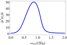
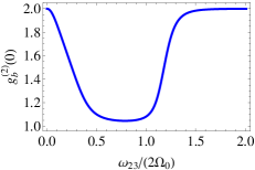
Figure 2: (a) The mean quanta number of the quantum oscillator $\langle b^{\dagger}b\rangle/\bar{n}$ and (b) its second-order correlation function $g^{(2)}_{b}(0)$ versus $\omega_{23}/(2\Omega_{0})$ for the situation (I). Here $g/\gamma_{2}=4$, $\gamma_{3}/\gamma_{2}=0.1$, $\gamma/\gamma_{2}=0$, $\kappa/\gamma_{2}=10^{-3}$, $\omega/\gamma_{2}=50$, $\Omega_{0}/\gamma_{2}=20$ and $\bar{n}=1$.

In order to solve the infinite system of Eq. (13), we truncate it at a certain maximum value $n=n_{max}$ so that a further increase of its value, i.e. $n_{max}$, does not modify the obtained results. Thus, the steady-state mean quanta’s number is expressed as:

$$\langle b^{\dagger}b\rangle=\sum^{n_{max}}_{n=0}nP_{n}^{(0)},$$ (14)

with

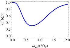
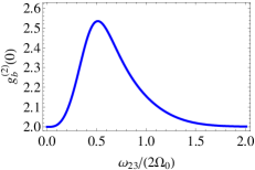
Figure 3: (a) The scaled mean quanta number of the quantum oscillator $\langle b^{\dagger}b\rangle/\bar{n}$ and (b) the corresponding second-order correlation function $g^{(2)}_{b}(0)$ against the scaled control parameter $\omega_{23}/(2\Omega_{0})$ for the situation (I). Here $g/\gamma_{3}=4$, $\gamma_{2}/\gamma_{3}=0.1$, $\gamma/\gamma_{3}=0$, $\kappa/\gamma_{3}=10^{-3}$, $\omega/\gamma_{3}=50$, $\Omega_{0}/\gamma_{3}=20$ and $\bar{n}=15$.

$$\sum^{n_{max}}_{n=0}P_{n}^{(0)}=1,$$ (15)

while its steady-state second-order correlation function is defined as usual glauber , namely,

$$g^{(2)}_{b}(0) = \frac{\langle b^{\dagger}b^{\dagger}bb\rangle}{\langle b^{\dagger}b\rangle^{2}}$$ (16)

$$= \frac{1}{\langle b^{\dagger}b\rangle^{2}}\sum^{n_{max}}_{n=0}n(n-1)P_{n}^{(0)}.$$

Respectively, the steady-state mean value of the dressed-state inversion operator, $\langle R_{z}\rangle=\langle R_{22}\rangle-\langle R_{33}\rangle$, can be obtained as follows:

$$\langle R_{z}\rangle=\sum^{n_{max}}_{n=0}P^{(2)}_{n}.$$ (17)

Figure (2) shows the steady-state behaviors of the mean quanta number and its quantum statistics based on Eqs. (13) and Exps. (14,15,16). The maximum for $\langle b^{\dagger}b\rangle$ occurs around $\bar{\delta}=0$, i.e., at the resonance when the quanta’s frequency $\omega$ equals the dressed-state splitting frequency $2\Omega$ due to pumping lasers. Importantly here, the quanta’s statistics is near Poissonian meaning that we have obtained lasing regimes in our system, see Figs. 2(a,b). Also, lasing is taking place if $\gamma_{3}/\gamma_{2}\ll 1$. In this case $\langle R_{22}\rangle>\langle R_{33}\rangle$, that is, we have dressed-state population inversion and this is the reason for lasing effect, see Fig. 6(a). To avoid any confusion via lasing we mean generation of quantum oscillator’s quanta possessing Poissonian statistics, i.e., $g^{(2)}_{b}(0)=1$. Respectively, Figure (3) depicts the cooling regimes in this system, under situation (I). This happens when $\gamma_{2}/\gamma_{3}\ll 1$ meaning that $\langle R_{22}\rangle<\langle R_{33}\rangle$ leading to quanta’s absorption processes, see Fig. 6(b). The minimum in the mean quanta number followed by an increased second-order correlation function $g^{(2)}_{b}(0)$ occur around $\bar{\delta}=0$, that is, at resonance condition, see Figs. 3(a,b).

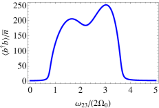
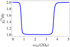
Figure 4: (a) The mean quanta number of the quantum oscillator $\langle b^{\dagger}b\rangle/\bar{n}$ and (b) its second-order correlation function $g^{(2)}_{b}(0)$ versus $\omega_{23}/(2\Omega_{0})$ for the situation (II) with $\gamma_{3}/\gamma_{2}\ll 1$. All other parameters are as in Figure (2).

Further, for the sake of comparison, we will keep the same parameters and shall investigate the quantum dynamics for the second situation, i.e. $(II)$. The respective equations of motion describing the quantum oscillator’s dynamics as well as the quantum emitter’s one are given in Appendix B, i.e., Eqs. (LABEL:aa1). Particularly, Fig. 4(a) shows the mean quanta’s number of the quantum oscillator in this case, whereas Fig. 4(b) depicts the corresponding behavior of the second-order quanta’s correlation function as a function of $\omega_{23}/(2\Omega_{0})$ when $\gamma_{3}/\gamma_{2}\ll 1$. Remarkably, one can observe a wide plateau where the quanta’s statistics is Poissonian while its quantum oscillator’s mean quanta number vary from small to larger numbers. Thus, we have a clear lasing effect in this setup. Compared with the corresponding case, but for the first situation (I), i.e. Fig. (2), here, there are generated more quanta of the quantum oscillator followed by a broader lasing regime which is more convenient for potential applications, see Fig. (4) and Fig. (2). In this context, if the upper state $|1\rangle$ of the three-level emitter has a permanent dipole then it can couple with a single cavity electromagnetic field mode of terahertz frequency, for instance. In this case, we have obtained a coherent electromagnetic field source generating terahertz photons. Regarding external applied field intensities $I$: For transition wavelengths of the order of $1\mu m$, spontaneous decay rates within the range $10^{9}-10^{10}$Hz, and the corresponding THz interval for the Rabi frequencies $\Omega\sim 10^{11}-10^{12}$Hz, one obtains $I$ within few to several $kW/cm^{2}$ which correspond to moderate laser intensities. Respectively, Fig. 5(a) emphasizes the cooling regime in the examined system, and for the second situation $(II)$, occurring when $\gamma_{2}/\gamma_{3}\ll 1$. The second-order correlation function increases respectively, see Fig. 5(b), demonstrating enhanced phonon-phonon or photon-photon correlations depending on the model we have in mind. Compared with Fig. (3) describing same things but for the first situation (I), the cooling is significantly enhanced in the second case $(II)$ while keeping identical parameters, see Fig. (5) and Fig. (3). The steady-state mean value of dressed-state inversion operator $\langle R_{z}\rangle$, in the lasing regime, behave differently in this case, compare Fig. 7(a) with Fig. 6(a). In the second situation (II), $\langle R_{z}\rangle$ approaches zero values, while the mean quanta’s number is large, although has a minimum, see Fig. 4(a). As we shall explain below, these behaviors are due to quantum interference effects. However, cooling occurs for $\langle R_{22}\rangle<\langle R_{33}\rangle$ facilitating quanta’s absorption processes, see Fig. 7(b). Note that we have carefully checked the convergence of our results with respect to various values for $n_{max}$.

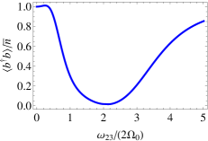
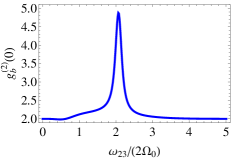
Figure 5: (a) The scaled mean quanta number of the quantum oscillator $\langle b^{\dagger}b\rangle/\bar{n}$ and (b) its second-order correlation function $g^{(2)}_{b}(0)$ versus $\omega_{23}/(2\Omega_{0})$ for the situation (II) with $\gamma_{2}/\gamma_{3}\ll 1$. All other parameters are as in Figure (3).

Although both situations $(I)$ and $(II)$ show cooling or lasing phenomena, the mechanisms behind them are completely different. If $\gamma_{2}\not=\gamma_{3}$ and $\gamma=0$, the first situation $(I)$ resembles a two-level system $\{|\Psi_{2}\rangle,|\Psi_{3}\rangle\}$ of frequency $2\Omega$ interacting, respectively, with a quantum oscillator of frequency $\omega$, with $2\Omega\approx\omega$, see also d_las . The spontaneous decay acts in both directions, i.e. $|\Psi_{2}\rangle\leftrightarrow|\Psi_{3}\rangle$, with a corresponding impact on cooling or lasing effects. The cross-correlation terms from the Master Equation (18) do not influence the quantum dynamics in this case from the simply reason that they do not enter at all in the equations of motion (13). On the other side, the second situation $(II)$ is close to an equidistant three-level system $|\Psi_{2}\rangle\leftrightarrow|\Psi_{1}\rangle\leftrightarrow|\Psi_{3}\rangle$, where each transition being of frequency $\Omega$ interacts as well with the quantum oscillator possessing the frequency $\omega$, however, with $\Omega\approx\omega$. In this case transitions may take place via single oscillator’s quanta processes among the dressed-state $|\Psi_{2}\rangle\leftrightarrow|\Psi_{1}\rangle\leftrightarrow|\Psi_{3}\rangle$ or, respectively, involving two-quanta effects among the dressed-states $|\Psi_{2}\rangle\leftrightarrow|\Psi_{3}\rangle$. This also means that cross-correlation terms from the Master Equation (18) do influence the quantum dynamics in this case. This is clearly elucidated also if one inspects the variables $\rho^{(i)},\{i\in 0\cdots 16\}$, given in the Appendix B, since it contain single or two-quanta processes appearing concomitantly. The various decay paths among the dressed-states involved $|\Psi_{2}\rangle\leftrightarrow|\Psi_{1}\rangle\leftrightarrow|\Psi_{3}\rangle$ lead to quantum interference effects, see also Eq. (18), although the dipole moments corresponding to the two bare transitions of the $\Lambda-$type sample are orthogonal to each other. These cross-correlations agarwal ; ficek_book ; kiffner among the dressed-states contribute to a more flexible domain for lasing and deeper cooling regimes compared to the situation $(I)$ and for the same parameters involved. Thus, one can conclude that quantum interference effects via single- or two-quanta processes distinguish the situation $(II)$, described by the Hamiltonian (12), from the corresponding one characterized by the Hamiltonian (11), i.e., the case $(I)$. This is also the reason that the three-level emitter’s population dynamics behave differently as well in these two cases, compare Fig. (6) and Fig. (7). Notice that when $\omega_{23}/2\Omega_{0}\to 0$ then the quantum emitter lies in the state $|\Psi\rangle=\bigl{(}|3\rangle-|2\rangle\bigr{)}/\sqrt{2}$, whereas $\langle b^{\dagger}b\rangle/\bar{n}=1$ and $g^{(2)}_{b}(0)=2$, see Figs. (2-5), meaning that the quantum oscillator’s mode is in a thermal state and no cooling or lasing effects take place, respectively. Here, these phenomena occur for $\omega_{23}/2\Omega_{0}\not=0$, when some population resides on the higher upper state $|1\rangle$, which is distinct from other related schemes based, however, on coherent population trapping effects or electromagnetically induced transparency phenomenon gxl1 ; gxl2 ; plenio2 ; plenio3 . Furthermore, we have observed that there are no cooling effects for both cases described here, $(I)$ or $(II)$, if $\gamma_{2}=\gamma_{3}$ while $\gamma=0$. However, the phenomenon it will appear as you increases $\gamma$ while keeping $\gamma_{2}=\gamma_{3}$. Finally, the temperatures ranges considered here are within several Kelvins for phonon cooling effects to few hundreds of Kelvins for coherent THz photon generation, respectively.

IV Summary

Summarizing, we have investigated a laser-pumped three-level $\Lambda-$type system the upper state of which is being coupled with a quantum oscillator characterized by a single quantized leaking mode. We have identified two distinct situations leading to cooling or lasing effects of the quantum oscillator’s degrees of freedom and have described the mechanisms behind them. Particularly, we have demonstrated that the interplay between single- or two-quanta processes accompanied by quantum interference effects among the induced emitter’s dressed-states are responsible for flexible lasing or deeper cooling effects, respectively. This leads also to mutual influences between the quantum oscillator’s dynamics and the three-level emitter’s quantum dynamics, respectively. The coherent terahertz photons generation is identified as one of the possible application resulting from this study.

Appendix A The master equation

Below, one can find the final Master Equation used to obtain the corresponding equations of motion describing the quantum dynamics of both the quantum oscillator as well as of the three-level $\Lambda-$type emitter, that is,

$$\dot{\rho} + \frac{i}{\hbar}[H,\rho]=-\gamma_{2}[R^{(+)},R^{(+)}\rho]-\gamma_{3}[R^{(-)},R^{(-)}\rho]$$ (18)

$$- \frac{\sin^{2}{\theta}}{4}\gamma^{(+)}[R_{12},R_{21}\rho]-\frac{\sin^{2}{\theta}}{4}\gamma^{(-)}[R_{13},R_{31}\rho]$$

$$- \gamma^{(0)}_{0}\bigl{(}[R_{21},R_{12}\rho]+[R_{31},R_{13}\rho]\bigr{)}-\Gamma^{(+)}[R_{32},R_{23}\rho]$$

$$- \Gamma^{(-)}[R_{23},R_{32}\rho]-\frac{\gamma^{(+)}_{0}}{2}\bigl{(}[R_{12},R_{13}\rho]+[R_{31},R_{21}\rho]\bigr{)}$$

$$- \frac{\gamma^{(-)}_{0}}{2}\bigl{(}[R_{21},R_{31}\rho]+[R_{13},R_{12}\rho]\bigr{)}-\frac{\gamma}{4}\cos^{4}{\theta}$$

$$\times [\frac{1}{2}(R_{22}+R_{33})-R_{11},\bigl{(}\frac{1}{2}(R_{22}+R_{33})-R_{11}\bigr{)}\rho]$$

$$- \frac{\gamma}{8}\cos^{2}{\theta}(1-\sin{\theta})^{2}[R_{12}+R_{31},(R_{21}+R_{13})\rho]$$

$$- \frac{\gamma}{8}\cos^{2}{\theta}(1+\sin{\theta})^{2}[R_{21}+R_{13},(R_{12}+R_{31})\rho]$$

$$- \kappa(1+\bar{n})[b^{\dagger},b\rho]-\kappa\bar{n}[b,b^{\dagger}\rho]+H.c.,$$

where $R^{(\pm)}$=$\frac{\sin{2\theta}}{2\sqrt{2}}R_{11}\mp\frac{\cos{\theta}}{2\sqrt{2}}(1\pm\sin{\theta})R_{22}\pm\frac{\cos{\theta}}{2\sqrt{2}}(1\mp\sin{\theta})R_{33}$. The following terms: $[R_{12},R_{13}\rho]$, $[R_{31},R_{21}\rho]$ $[R_{21},R_{31}\rho]$ and $[R_{13},R_{12}\rho]$ as well as their Hermitian conjugate parts characterize the cross-damping effects or quantum interference phenomena agarwal ; ficek_book ; kiffner . As an exercise, we present the equations of motion for the dressed-state populations of the three-level emitter in the absence of the quantum oscillator, that is $g=0$,

$$\langle\dot{R}_{22}\rangle = \gamma^{(+)}_{11}\langle R_{11}\rangle-\gamma^{(+)}_{22}\langle R_{22}\rangle+\gamma^{(+)}_{33}\langle R_{33}\rangle,$$

$$\langle\dot{R}_{33}\rangle = \gamma^{(-)}_{11}\langle R_{11}\rangle+\gamma^{(-)}_{33}\langle R_{22}\rangle-\gamma^{(-)}_{22}\langle R_{33}\rangle,$$

$$\langle R_{11}\rangle = 1-\langle R_{22}\rangle-\langle R_{33}\rangle.$$ (19)

Here, $\gamma^{(\pm)}_{11}=\gamma^{(\pm)}\sin^{2}{\theta}/2+\gamma\cos^{2}{\theta}(1\mp\sin{\theta})^{2}/4$, $\gamma^{(\pm)}_{22}=2\gamma^{(0)}_{0}+\Gamma^{(\mp)}/2+\gamma\cos^{2}{\theta}(1\pm\sin{\theta})^{2}/4$ and $\gamma^{(\pm)}_{33}=\gamma^{(\pm)}\cos^{2}{\theta}/4+\gamma(1\mp\sin{\theta})^{4}/8$. One can observe that the cross-correlation terms from the Master Equation (18) do not contribute to population quantum dynamics given by Eqs. (19). However, their influence will appear in the presence of the quantum oscillator, i.e. when $g\not=0$, and this is clearly shown here, compare Fig. (6) and Fig. (7). The steady-state solutions of the above system of equations are:

$$\langle R_{22}\rangle = \bigl{(}\gamma^{(+)}_{11}\gamma^{(-)}_{22}+\gamma^{(-)}_{11}\gamma^{(+)}_{33}\bigr{)}/\bigl{(}\gamma^{(+)}_{11}(\gamma^{(-)}_{22}+\gamma^{(-)}_{33})$$

$$+ \gamma^{(+)}_{22}(\gamma^{(-)}_{11}+\gamma^{(-)}_{22})+\gamma^{(+)}_{33}(\gamma^{(-)}_{11}-\gamma^{(-)}_{33})\bigr{)},$$

whereas the solution for $\langle R_{33}\rangle$ can be obtained from Exp. (LABEL:ssqp) via an exchange of upper signs, i.e. $(\pm)\to(\mp)$.

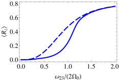
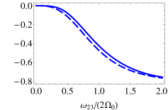
Figure 6: The mean dressed-state inversion operator $\langle R_{z}\rangle=\langle R_{22}\rangle-\langle R_{33}\rangle$ as a function of $\omega_{23}/(2\Omega_{0})$ obtained in the steady-state for the first situation (I). (a) $\gamma_{3}/\gamma_{2}\ll 1$ whereas (b) $\gamma_{2}/\gamma_{3}\ll 1$. The solid lines are obtained with the full system of equations (13), while the dashed lines in the absence of the quantum oscillator, i.e. with Exp. (LABEL:ssqp). All other parameters are as in Fig. (2) and Fig. (3), respectively.

Fig. (6) and Fig. (7) depict the steady-state values of the dressed-state inversion operator $\langle R_{z}\rangle$ for the both cases studied here, $(I)$ and $(II)$, and in the presence of the quantum oscillator (solid lines) as well as in its absence (dashed curves), respectively. One can observe that there is a clear difference between the cases with $g=0$ and $g\not=0$ in the lasing regimes, compare Fig. 6(a) and Fig. 7(a). As it was described above, this distinction is due to cross-correlation terms or quantum interference effects arising in the second case (II). Correspondingly, in the cooling regimes the quantum oscillator’s influence on the steady-state mean value of the qubit inversion operator is not quite significant, although still visible.

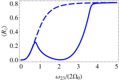
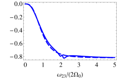
Figure 7: The same as in Fig. (6) but for the second case (II). The solid lines are obtained with the full system of equations of motion (LABEL:aa1), while the dashed lines with Exp. (LABEL:ssqp). All other parameters are as in Fig. (4) and Fig. (5), respectively.

Appendix B The equations of motion when $\omega\approx\Omega$, i.e., for the case (II)

Here, we shall present the equations of motion for the second situation $(II)$ obtained with the help of the Master Equation (18), that is,

$$\dot{P}^{(0)}_{n} = i\tilde{g}(P^{(3)}_{n}-P^{(5)}_{n}-P^{(9)}_{n}+P^{(7)}_{n})-2\kappa\bar{n}\bigl{(}(n+1)P^{(0)}_{n}$$

$$- nP^{(0)}_{n-1}\bigr{)}-2\kappa(1+\bar{n})\bigl{(}nP^{(0)}_{n}-(n+1)P^{(0)}_{n+1}\bigr{)},$$

$$\dot{P}^{(1)}_{n} = i\tilde{g}(P^{(7)}_{n}-P^{(9)}_{n})-2\kappa\bar{n}\bigl{(}(n+1)P^{(1)}_{n}-nP^{(1)}_{n-1}\bigr{)}$$

$$- 2\kappa(1+\bar{n})\bigl{(}nP^{(1)}_{n}-(n+1)P^{(1)}_{n+1}\bigr{)}+\tilde{\gamma}^{(1)}_{0}P^{(0)}_{n}$$

$$- \tilde{\gamma}^{(1)}_{1}P^{(1)}_{n}-\tilde{\gamma}^{(1)}_{2}P^{(2)}_{n},$$

$$\dot{P}^{(2)}_{n} = -i\tilde{g}(P^{(9)}_{n}+P^{(7)}_{n})-2\kappa\bar{n}\bigl{(}(n+1)P^{(2)}_{n}-nP^{(2)}_{n-1}\bigr{)}$$

$$- 2\kappa(1+\bar{n})\bigl{(}nP^{(2)}_{n}-(n+1)P^{(2)}_{n+1}\bigr{)}+\tilde{\gamma}^{(2)}_{0}P^{(0)}_{n}$$

$$+ \tilde{\gamma}^{(2)}_{1}P^{(1)}_{n}-\tilde{\gamma}^{(2)}_{2}P^{(2)}_{n},$$

$$\dot{P}^{(3)}_{n} = i\tilde{\delta}P^{(4)}_{n}-\tilde{\gamma}^{(3)}_{3}P^{(3)}_{n}+\tilde{\gamma}^{(3)}_{7}P^{(7)}_{n}$$

$$+ i\tilde{g}(n(2P^{(0)}_{n}-P^{(1)}_{n-1}-P^{(2)}_{n-1})-(2n+1)P^{(1)}_{n})$$

$$- \kappa(1+\bar{n})\bigl{(}(2n-1)P^{(3)}_{n}-2(n+1)P^{(3)}_{n+1}$$

$$+ 2P^{(9)}_{n}\bigr{)}-\kappa\bar{n}\bigl{(}(2n+1)P^{(3)}_{n}-2nP^{(3)}_{n-1}\bigr{)},$$

$$\dot{P}^{(4)}_{n} = i\tilde{\delta}P^{(3)}_{n}-i\tilde{g}P^{(12)}_{n}-\kappa(1+\bar{n})\bigl{(}(2n-1)P^{(4)}_{n}$$

$$+ 2P^{(10)}_{n}-2(n+1)P^{(4)}_{n+1}\bigr{)}-\kappa\bar{n}\bigl{(}(2n+1)P^{(4)}_{n}$$

$$- 2nP^{(4)}_{n-1}\bigr{)}-\tilde{\gamma}^{(4)}_{4}P^{(4)}_{n}+\tilde{\gamma}^{(4)}_{8}P^{(8)}_{n},$$

$$\dot{P}^{(5)}_{n} = i\tilde{\delta}P^{(6)}_{n}+i\tilde{g}\bigl{(}P^{(11)}_{n}+(n+1)(P^{(1)}_{n+1}-P^{(2)}_{n+1})$$

$$- 2(n+1)(P^{(0)}_{n}-P^{(1)}_{n})\bigr{)}$$

$$- \kappa(1+\bar{n})\bigl{(}(2n+1)P^{(5)}_{n}-2(n+1)P^{(5)}_{n+1}\bigr{)}$$

$$- \kappa\bar{n}\bigl{(}(2n+3)P^{(5)}_{n}-2nP^{(5)}_{n-1}-2P^{(7)}_{n}\bigr{)}$$

$$- \tilde{\gamma}^{(5)}_{5}P^{(5)}_{n}+\tilde{\gamma}^{(5)}_{9}P^{(9)}_{n},$$

$$\dot{P}^{(6)}_{n} = i\tilde{\delta}P^{(5)}_{n}+i\tilde{g}P^{(12)}_{n}-\kappa\bar{n}\bigl{(}(2n+3)P^{(6)}_{n}-2nP^{(6)}_{n-1}$$

$$- 2P^{(8)}_{n}\bigr{)}-\kappa(1+\bar{n})\bigl{(}(2n+1)P^{(6)}_{n}-2(n+1)$$

$$\times P^{(6)}_{n+1}\bigr{)}-\tilde{\gamma}^{(6)}_{6}P^{(6)}_{n}+\tilde{\gamma}^{(6)}_{10}P^{(10)}_{n},$$

$$\dot{P}^{(7)}_{n} = i\tilde{\delta}P^{(8)}_{n}+i\tilde{g}\bigl{(}P^{(13)}_{n}+n(P^{(1)}_{n}-P^{(2)}_{n})-2n(P^{(0)}_{n-1}$$

$$- P^{(1)}_{n-1})\bigr{)}-\kappa\bar{n}\bigl{(}(2n+1)P^{(7)}_{n}-2nP^{(7)}_{n-1}\bigr{)}$$

$$- \kappa(1+\bar{n})\bigl{(}(2n-1)P^{(7)}_{n}-2(n+1)P^{(7)}_{n+1}$$

$$+ 2P^{(5)}_{n}\bigr{)}+\tilde{\gamma}^{(7)}_{3}P^{(3)}_{n}-\tilde{\gamma}^{(7)}_{7}P^{(7)}_{n},$$

$$\dot{P}^{(8)}_{n} = i\tilde{\delta}P^{(7)}_{n}+i\tilde{g}P^{(14)}_{n}-\kappa\bar{n}\bigl{(}(2n+1)P^{(8)}_{n}-2nP^{(8)}_{n-1}\bigr{)}$$

$$- \kappa(1+\bar{n})\bigl{(}(2n-1)P^{(8)}_{n}-2(n+1)P^{(8)}_{n+1}$$

$$+ 2P^{(6)}_{n}\bigr{)}+\tilde{\gamma}^{(8)}_{4}P^{(4)}_{n}-\tilde{\gamma}^{(8)}_{8}P^{(8)}_{n},$$

$$\dot{P}^{(9)}_{n} = i\tilde{\delta}P^{(10)}_{n}+i\tilde{g}\bigl{(}2(n+1)(P^{(0)}_{n+1}-P^{(1)}_{n+1})-(n+1)$$

$$\times (P^{(1)}_{n}+P^{(2)}_{n})-P^{(15)}_{n}\bigr{)}-\kappa(1+\bar{n})\bigl{(}(2n+1)P^{(9)}_{n}$$

$$- 2(n+1)P^{(9)}_{n+1}\bigr{)}-\kappa\bar{n}\bigl{(}(2n+3)P^{(9)}_{n}-2nP^{(9)}_{n-1}$$

$$- 2P^{(3)}_{n}\bigr{)}+\tilde{\gamma}^{(9)}_{5}P^{(5)}_{n}-\tilde{\gamma}^{(9)}_{9}P^{(9)}_{n},$$

$$\dot{P}^{(10)}_{n} = i\tilde{\delta}P^{(9)}_{n}-i\tilde{g}P^{(16)}_{n}-\kappa\bar{n}\bigl{(}(2n+3)P^{(10)}_{n}-2nP^{(10)}_{n-1}$$

$$- 2P^{(4)}_{n}\bigr{)}-\kappa(1+\bar{n})\bigl{(}(2n+1)P^{(10)}_{n}-2(n+1)$$

$$\times P^{(10)}_{n+1}\bigr{)}+\tilde{\gamma}^{(10)}_{6}P^{(6)}_{n}-\tilde{\gamma}^{(10)}_{10}P^{(10)}_{n},$$

$$\dot{P}^{(11)}_{n} = 2i\tilde{\delta}P^{(12)}_{n}+i\tilde{g}\bigl{(}nP^{(5)}_{n}-(n+1)P^{(3)}_{n}\bigr{)}-2\kappa(1+\bar{n})$$

$$\times \bigl{(}nP^{(11)}_{n}-(n+1)P^{(11)}_{n+1}+P^{(15)}_{n}\bigr{)}-2\kappa\bar{n}\bigl{(}(n+1)$$

$$\times P^{(11)}_{n}-nP^{(11)}_{n-1}-P^{(13)}_{n}\bigr{)}-\tilde{\gamma}^{(11)}_{11}P^{(11)}_{n},$$

$$\dot{P}^{(12)}_{n} = 2i\tilde{\delta}P^{(11)}_{n}+i\tilde{g}\bigl{(}nP^{(6)}_{n}-(n+1)P^{(4)}_{n}\bigr{)}-2\kappa(1+\bar{n})$$

$$\times \bigl{(}nP^{(12)}_{n}-(n+1)P^{(12)}_{n+1}+P^{(16)}_{n}\bigr{)}-2\kappa\bar{n}\bigl{(}(n+1)$$

$$\times P^{(12)}_{n}-nP^{(12)}_{n-1}-P^{(14)}_{n}\bigr{)}-\tilde{\gamma}^{(12)}_{12}P^{(12)}_{n},$$

$$\dot{P}^{(13)}_{n} = 2i\tilde{\delta}P^{(14)}_{n}+i\tilde{g}\bigl{(}(n-1)P^{(7)}_{n}-nP^{(3)}_{n-1}\bigr{)}-2\kappa(1+\bar{n})$$

$$\times \bigl{(}(n-1)P^{(13)}_{n}-(n+1)P^{(13)}_{n+1}+2P^{(11)}_{n}\bigr{)}-2\kappa n\bar{n}$$

$$\times \bigl{(}P^{(13)}_{n}-P^{(13)}_{n-1}\bigr{)}-\tilde{\gamma}^{(13)}_{13}P^{(13)}_{n},$$

$$\dot{P}^{(14)}_{n} = 2i\tilde{\delta}P^{(13)}_{n}+i\tilde{g}\bigl{(}(n-1)P^{(8)}_{n}-nP^{(4)}_{n-1}\bigr{)}-2\kappa(1+\bar{n})$$

$$\times \bigl{(}(n-1)P^{(14)}_{n}-(n+1)P^{(14)}_{n+1}+2P^{(12)}_{n}\bigr{)}-2\kappa n\bar{n}$$

$$\times \bigl{(}P^{(14)}_{n}-P^{(14)}_{n-1}\bigr{)}-\tilde{\gamma}^{(14)}_{14}P^{(14)}_{n},$$

$$\dot{P}^{(15)}_{n} = 2i\tilde{\delta}P^{(16)}_{n}+i\tilde{g}\bigl{(}(n+1)P^{(5)}_{n}-(n+2)P^{(9)}_{n}\bigr{)}$$

$$- 2\kappa(1+\bar{n})(1+n)\bigl{(}P^{(15)}_{n}-P^{(15)}_{n+1}\bigr{)}-2\kappa\bar{n}$$

$$\times \bigl{(}(n+2)P^{(15)}_{n}-nP^{(15)}_{n-1}-2P^{(11)}_{n}\bigr{)}-\tilde{\gamma}^{(15)}_{15}P^{(15)}_{n},$$

$$\dot{P}^{(16)}_{n} = 2i\tilde{\delta}P^{(15)}_{n}+i\tilde{g}\bigl{(}(n+1)P^{(6)}_{n+1}-(n+2)P^{(10)}_{n}\bigr{)}$$

$$- 2\kappa(1+\bar{n})(1+n)\bigl{(}P^{(16)}_{n}-P^{(16)}_{n+1}\bigr{)}-2\kappa\bar{n}$$

$$\times \bigl{(}(n+2)P^{(16)}_{n}-nP^{(16)}_{n-1}-2P^{(12)}_{n}\bigr{)}-\tilde{\gamma}^{(16)}_{16}P^{(16)}_{n}.$$

Here $\tilde{\gamma}^{(1)}_{0}=\gamma^{(1)}_{0}$, $\tilde{\gamma}^{(1)}_{1}=\gamma^{(1)}_{1}$, $\tilde{\gamma}^{(1)}_{2}=\gamma\sin{\theta}\cos^{2}{\theta}/2$, $\tilde{\gamma}^{(2)}_{0}=\gamma^{(2)}_{0}$, $\tilde{\gamma}^{(2)}_{1}=-\gamma^{(2)}_{1}$, $\tilde{\gamma}^{(2)}_{2}=\gamma^{(2)}_{2}$, $\tilde{\gamma}^{(3)}_{3}=\gamma_{2}\cos^{2}{\theta}(1+3\sin{\theta})^{2}/8$ + $\gamma_{3}\cos^{2}{\theta}(1-3\sin{\theta})^{2}/8$ + $(\gamma^{(+)}+\gamma^{(-)})\sin^{2}{\theta}/4+\gamma^{(0)}_{0}+\Gamma^{(-)}$ + $9\gamma\cos^{4}{\theta}/16$ + $\gamma\cos^{2}{\theta}\bigl{(}(1+\sin{\theta})^{2}+(1-\sin{\theta})^{2}/2\bigr{)}/4$, $\tilde{\gamma}^{(3)}_{7}=\gamma^{(+)}_{0}+\gamma\cos^{2}{\theta}(1-\sin{\theta})^{2}/4$, $\tilde{\gamma}^{(4)}_{4}=\tilde{\gamma}^{(3)}_{3}$, $\tilde{\gamma}^{(4)}_{8}=\tilde{\gamma}^{(3)}_{7}$, $\tilde{\gamma}^{(5)}_{5}=\gamma_{2}\cos^{2}{\theta}(1-3\sin{\theta})^{2}/8$ + $\gamma_{3}\cos^{2}{\theta}(1+3\sin{\theta})^{2}/8$ + $(\gamma^{(+)}+\gamma^{(-)})\sin^{2}{\theta}/4+\gamma^{(0)}_{0}+\Gamma^{(+)}$ + $9\gamma\cos^{4}{\theta}/16$ + $\gamma\cos^{2}{\theta}\bigl{(}(1-\sin{\theta})^{2}+(1+\sin{\theta})^{2}/2\bigr{)}/4$, $\tilde{\gamma}^{(5)}_{9}=\gamma^{(-)}_{0}+\gamma\cos^{2}{\theta}(1+\sin{\theta})^{2}/4$, $\tilde{\gamma}^{(6)}_{6}=\tilde{\gamma}^{(5)}_{5}$, $\tilde{\gamma}^{(6)}_{10}=\tilde{\gamma}^{(5)}_{9}$, $\tilde{\gamma}^{(7)}_{7}=\tilde{\gamma}^{(6)}_{6}$, $\tilde{\gamma}^{(7)}_{3}=\tilde{\gamma}^{(6)}_{10}$, $\tilde{\gamma}^{(8)}_{8}=\tilde{\gamma}^{(7)}_{7}$, $\tilde{\gamma}^{(8)}_{4}=\tilde{\gamma}^{(7)}_{3}$, $\tilde{\gamma}^{(9)}_{5}=\gamma^{(+)}_{0}+\gamma\cos^{2}{\theta}(1-\sin{\theta})^{2}/4$, $\tilde{\gamma}^{(9)}_{9}=\tilde{\gamma}^{(3)}_{3}=\tilde{\gamma}^{(10)}_{10}$, $\tilde{\gamma}^{(10)}_{6}=\tilde{\gamma}^{(9)}_{5}$, $\tilde{\gamma}^{(11)}_{11}=(\gamma_{2}+\gamma_{3})\cos^{2}{\theta}/2+2\gamma^{(0)}_{0}+\Gamma^{(-)}+\Gamma^{(+)}+\gamma\cos^{2}{\theta}(1+\sin^{2}{\theta})/4$, and $\tilde{\gamma}^{(11)}_{11}=\tilde{\gamma}^{(12)}_{12}=\tilde{\gamma}^{(13)}_{13}=\tilde{\gamma}^{(14)}_{14}=\tilde{\gamma}^{(15)}_{15}=\tilde{\gamma}^{(16)}_{16}$.

The system of equations (LABEL:aa1) can be obtained if one first get the equations of motion for the variables: $\rho^{(0)}=\rho_{11}+\rho_{22}+\rho_{33}$, $\rho^{(1)}=\rho_{22}+\rho_{33}$, $\rho^{(2)}=\rho_{22}-\rho_{33}$, $\rho^{(3)}=b^{\dagger}\rho_{21}-\rho_{12}b$, $\rho^{(4)}=b^{\dagger}\rho_{21}+\rho_{12}b$, $\rho^{(5)}=\rho_{13}b^{\dagger}-b\rho_{31}$, $\rho^{(6)}=\rho_{13}b^{\dagger}+b\rho_{31}$, $\rho^{(7)}=b^{\dagger}\rho_{13}-\rho_{31}b$, $\rho^{(8)}=b^{\dagger}\rho_{13}+\rho_{31}b$, $\rho^{(9)}=\rho_{21}b^{\dagger}-b\rho_{12}$, $\rho^{(10)}=\rho_{21}b^{\dagger}+b\rho_{12}$, $\rho^{(11)}=b^{\dagger}\rho_{23}b^{\dagger}+b\rho_{32}b$, $\rho^{(12)}=b^{\dagger}\rho_{23}b^{\dagger}-b\rho_{32}b$, $\rho^{(13)}=b^{\dagger 2}\rho_{23}+\rho_{32}b^{2}$, $\rho^{(14)}=b^{\dagger 2}\rho_{23}-\rho_{32}b^{2}$, $\rho^{(15)}=\rho_{23}b^{\dagger 2}+b^{2}\rho_{32}$, $\rho^{(16)}=\rho_{23}b^{\dagger 2}-b^{2}\rho_{32}$, using the Master Equation (18) and then projecting them on the Fock states $|n\rangle$, i.e., $P^{(i)}_{n}=\langle n|\rho^{(i)}|n\rangle$, $\{i\in 0\cdots 16\}$, and $n\in\{0,\infty\}$. Together with Exps. (14,15,16,17,LABEL:ssqp) one can obtain the interested quantities like the mean quanta’s number of the quantum oscillator or its quantum statistics described by the second-order correlation function as well as qubit’s populations, see Figs. (4), (5), (6) and (7).

References

• (1) D. Leibfried, R. Blatt, C. Monroe, and D. Wineland, Quantum dynamics of single trapped ions, Rev. Mod. Phys. 75, 281 (2003).
• (2) M. Khajavikhan, A. Simic, M. Katz, J. H. Lee, B. Slutsky, A. Mizrahi, V. Lomakin, and Y. Fainman, Thresholdless nanoscale coaxial lasers, Nature 482, 204 (2012).
• (3) J. Zakrzewski, M. Lewenstein, and Th. W. Mossberg, Theory of dressed-state lasers. I. Effective Hamiltonians and stability properties, Phys. Rev. A 44, 7717 (1991).
• (4) I. Wilson-Rae, P. Zoller, and A. Imamoglu, Laser Cooling of a Nanomechanical Resonator Mode to its Quantum Ground State, Phys. Rev. Lett. 92, 075507 (2004).
• (5) J. Kabuss, A. Carmele, T. Brandes, and A. Knorr, Optically Driven Quantum Dots as Source of Coherent Cavity Phonons: A Proposal for a Phonon Laser Scheme, Phys. Rev. Lett. 109, 054301 (2012).
• (6) M. Fleischhauer, A. Imamoglu, and J. P. Marangos, Electromagnetically induced transparency: Optics in coherent media, Rev. Mod. Phys. 77, 633 (2005).
• (7) H. J. Kimble, The quantum internet, Nature 453, 1023 (2008).
• (8) D. D. Awschalom, R. Hanson, J. Wrachtrup, and B. B. Zhou, Quantum technologies with optically interfaced solid-state spins, Nature Photonics 12, 516 (2018).
• (9) G. Morigi, J. Eschner, and C. H. Keitel, Ground State Laser Cooling Using Electromagnetically Induced Transparency, Phys. Rev. Lett. 85, 4458 (2000).
• (10) C. F. Roos, D. Leibfried, A.Mundt, F. Schmidt-Kaler, J. Eschner, and R. Blatt, Experimental Demonstration of Ground State Laser Cooling with Electromagnetically Induced Transparency, Phys. Rev. Lett. 85, 5547 (2000).
• (11) J. Evers, and C. H. Keitel, Double-EIT ground-state laser cooling without blue-sideband heating, Europhys. Lett. 68, 370 (2004).
• (12) J. Cerrillo, A. Retzker, and M. B. Plenio, Fast and Robust Laser Cooling of Trapped Systems, Phys. Rev. Lett. 104, 043003 (2010).
• (13) Y. Greenberg, Y. Pashkin, and E. Il’ichev, Nanomechanical resonators, Phys. Usp. 55, 382 (2012).
• (14) M. Aspelmeyer, T. J. Kippenberg, and F. Marquardt, Cavity optomechanics, Rev. Mod. Phys. 86, 1391 (2014).
• (15) K. Xia, and J. Evers, Ground State Cooling of a Nanomechanical Resonator in the Nonresolved Regime via Quantum Interference, Phys. Rev. Lett. 103, 227203 (2009).
• (16) K. Vahala, M. Herrmann, S. Knünz, V. Batteiger, G. Saathoff, T. W. Hänsch, and Th. Udem, A phonon laser, Nature Physics 5, 682 (2009).
• (17) C. Schäfermeier, H. Kerdoncuff, U. B. Hoff, H. Fu, A. Huck, J. Bilek, G. I. Harris, W. P. Bowen, T. Gehring, and U. L. Andersen, Quantum enhanced feedback cooling of a mechanical oscillator using nonclassical light, Nature Communications 7:13628 (2016).
• (18) J. B. Clark, F. Lecocq, R. W. Simmonds, J. Aumentado, and J. D. Teufel, Sideband cooling beyond the quantum backaction limit with squeezed light, Nature 541, 191 (2017).
• (19) G. B. Serapiglia, E. Paspalakis, C. Sirtori, K. L. Vodopyanov, and C. C. Phillips, Laser-Induced Quantum Coherence in a Semiconductor Quantum Well, Phys. Rev. Lett. 84, 1019 (2000).
• (20) A. Beveratos, I. Abram, J.-M. Gerard, and I. Robert-Philip, Quantum optics with quantum dots: Towards semiconductor sources of quantum light for quantum information processing, Eur. Phys. J. D 68, 377 (2014).
• (21) V. Ceban, Phase-dependent quantum interferences with three-level artificial atoms, Romanian Journal of Physics 62, 207 (2017).
• (22) J.-p. Zhu, and G.-x. Li, Ground-state cooling of a nanomechanical resonator with a triple quantum dot via quantum interference, Phys. Rev. A 86, 053828 (2012).
• (23) G.-x. Li, and J.-p. Zhu, Ground-state cooling of a mechanical resonator coupled to two coupled quantum dots, J. Phys. B: At. Mol. Opt. Phys. 44, 195502 (2011).
• (24) H.-K. Lau, and M. B. Plenio, Laser cooling of a high-temperature oscillator by a three-level system, Phys. Rev. B 94, 054305 (2016).
• (25) M. Abdi, and M. B. Plenio, Quantum Effects in a Mechanically Modulated Single-Photon Emitter, Phys. Rev. Lett. 122, 023602 (2019).
• (26) V. Ceban, P. Longo, and M. A. Macovei, Fast phonon dynamics of a nanomechanical oscillator due to cooperative effects, Phys. Rev. A 95, 023806 (2017).
• (27) G. Ducournau, Terahertz science: Silicon photonics targets terahertz region, Nature Photonics 12, 574 (2018).
• (28) T. Harter, S. Muehlbrandt, S. Ummethala, A. Schmid, S. Nellen, L. Hahn, W. Freude, and C. Koos, Silicon–plasmonic integrated circuits for terahertz signal generation and coherent detection, Nature Photonics 12, 625 (2018).
• (29) Sh. Du, K. Yoshida, Ya Zhang, I. Hamada, and K. Hirakawa, Terahertz dynamics of electron–vibron coupling in single molecules with tunable electrostatic potential, Nature Photonics 12, 608 (2012).
• (30) O. V. Kibis, G. Ya. Slepyan, S. A. Maksimenko, and A. Hoffmann, Matter Coupling to Strong Electromagnetic Fields in Two-Level Quantum Systems with Broken Inversion Symmetry, Phys. Rev. Lett. 102, 023601 (2009).
• (31) F. Oster, C. H. Keitel, and M. Macovei, Generation of correlated photon pairs in different frequency ranges, Phys. Rev. A 85, 063814 (2012).
• (32) S. De Liberato, C. Ciuti and Ch. C. Phillips, Terahertz lasing from intersubband polariton-polariton scattering in asymmetric quantum wells, Phys. Rew. B 87, 241304(R) (2013).
• (33) M. Miri, F. Zamani, and H. Alipoor, Two tunneling-coupled two-level systems with broken inversion symmetry: tuning the terahertz emission, Jr. Opt. Soc. Am. B 33, 1873 (2016).
• (34) I. Yu. Chestnov, V. A. Shahnazaryan, A. P. Alodjants, and I. A. Shelykh, Terahertz Lasing in Ensemble of Asymmetric Quantum Dots, ACS Photonics 4(11), 2726 (2017).
• (35) M. Macovei, M. Mishra, and C. H. Keitel, Population inversion in two-level systems possessing permanent dipoles, Phys. Rev. A 92, 013846 (2015).
• (36) G. Yu. Kryuchkyan, V. Shahnazaryan, O. V. Kibis, and I. A. Shelykh, Resonance fluorescence from an asymmetric quantum dot dressed by a bichromatic electromagnetic field, Phys. Rev. A 95, 013834 (2017).
• (37) M. A. Anton, S. Maede-Razavi, F. Carreno, I. Thanopulos, and E. Paspalakis, Optical and microwave control of resonance fluorescence and squeezing spectra in a polar molecule, Phys. Rev. A 96, 063812 (2017).
• (38) D. Hiluf, and Y. Dubi, Phonon as environmental disturbance in three level system, arXiv:1803.08327v1.
• (39) F. Zhou, Y. Niu, and S. Gong, Electromagnetically induced transparency in a three-level lambda system with permanent dipole moments, J. Chem. Phys. 131, 034105 (2009).
• (40) S. Kocinac, Z. Ikonic, and V. Milanovic, Second Harmonic Generation at the Quantum-Interference Induced Transparency in Semiconductor Quantum Wells: The Influence of Permanent Dipole Moments, IEEE Jr. Quant. Electr. 37(7), 873 (2001).
• (41) G. S. Agarwal, Quantum Optics (Cambridge University Press, 2014).
• (42) C. W. Gardiner and P. Zoller, Quantum Noise (Springer, Berlin, 2004).
• (43) D. F. Walls and G. J. Milburn, Quantum Optics (Springer, Berlin, 2008).
• (44) T. Quang and H. Freedhoff, Atomic population inversion and enhancement of resonance fluorescence in a cavity, Phys. Rev. A 47, 2285 (1993).
• (45) R. J. Glauber, The Quantum Theory of Optical Coherence, Phys. Rev. 130, 2529 (1963).
• (46) G. S. Agarwal, Quantum Statistical Theories of Spontaneous Emission and their Relation to other Approaches (Springer, Berlin, 1974).
• (47) Z. Ficek and S. Swain, Quantum Interference and Coherence: Theory and Experiments (Springer, Berlin, 2005).
• (48) M. Kiffner, M. Macovei, J. Evers, and C. H. Keitel, Vacuum induced processes in multilevel atoms, Prog. Opt. 55, 85 (2010).