Discovery of the Odderon by TOTEM experiments and the FMO approach

Abstract

This paper is an extended version of the talk by B. Nicolescu at the XLVIII International Symposium on Multiparticle Dynamics (ISMD2018) at Singapore, 3-7 September, 2018. Theoretical basis and history of the Froissaron and Maximal Odderon (FMO) approach for elastic $pp$ and $\bar{p}p$ scattering is presented. Precise formulation of the FMO model at any momentum transfer squared $t$ is given. The model is applied to description and analysis of the experimental data in a wide interval of energy $\sqrt{s}$ and $t$. The special attention is given for the latest TOTEM data at 13 TeV, both at $t=0$ and at $t\neq 0$ and to their interpretation in the FMO model. It is emphasized that the last TOTEM results can be considered as clear evidence for the first experimental observation of the Odderon, predicted theoretically about 50 years ago.

1 Introduction

Recently, the TOTEM experiment released the following values at $\sqrt{s}=13$ TeV of $pp$ total cross section $\sigma^{pp}$ and $\rho^{pp}$ parameter TOTEM-1 ; TOTEM-2

$$\sigma^{pp}=110\pm 6\quad\text{mb},\qquad\rho^{pp}=0.098\pm 0.01\quad(0.10\pm 0.01)$$ (1)

The value of $\sigma^{pp}$ is in good agreement with the standard best COMPETE prediction COMPETE but is in violent disagreement with the COMPETE prediction for $\rho^{pp}$ (which is much higher than the experimental value). This is the first problem we have to solve before drawing conclusions about the discovery of the Odderon (which is absent in the COMPETE approach). On the other hand, the experimental value of $\rho^{pp}$ is in perfect agreement with the AvilaâGauronâNicolescu (AGN) model AGN , which includes the Odderon and which predicts a value of 0.105. In fact, the AGN model was the only model which correctly predicted $\rho^{pp}$ but it predicted also higher values of $\sigma^{pp}$ than the TOTEM values, a discrepancy which might be connected with the ambiguities in continuing the amplitudes in the non-forward region. This is the second problem we have to solve before drawing conclusions about the discovery of the Odderon. The third task is to extend the new FMO, model which fixes the first two problems, for $t\neq 0$ and to compare it with the newest TOTEM data on differential cross section at $\sqrt{s}=13$ TeV.

Part of this program was realized in the Refs. MN-0 ; MN-1 ; MN-2 . Here we give only the main, principal results obtained in this direction. Many additional results and details can be found in the refs. MN-0 ; MN-1 ; MN-2 .

2 Theoretical justification and history of the FMO approach

The aforementioned AGN model is not the only realization of Froissaron and Maximal Odderon (FMO) approach to high energy elastic hadron scattering. The general principles and basic strict results of Quantum Field Theory and Analytic $S$-matrix theory can not determine in an unique way the amplitudes of elastic scattering. At the same time they (many of them as well as references of original papers, where they have been obtained,can be found in review Eden ) strongly restrict the arbitrariness in construction of the models. Additional restrictions for the model are given by available experimental data.

In this Section we discuss the theoretical constraints which should be satisfied in any model of elastic scattering and some additional assumptions which lead to FMO-type models. Omitting the details of the strict results and assumptions we rather give the list of those that are important in Froissaron anf Maximal Odderon approach to high energy elastic scattering of hadrons (moreover we concentrate on $pp$ and $\bar{p}p$ elastic scattering.) As usually, as it is made for processes at high energy, we consider proton and antiproton as spin-less particles.

2.1 Rigorous results and assumptions important for FMO model

Froissart-Martin-Lukaszuk bound. It follows from unitarity and analyticity of amplitude that

$$\sigma_{t}(s)\leq C\ln^{2}(s/s_{0}),\qquad C\leq\dfrac{\pi}{m_{\pi}^{2}}.$$ (2)

Here and in what follows we take $s_{0}=1$ Gev.

In Regge theory the contribution of Regge pole with trajectory $\alpha(0)$ to the elastic scattering amplitude has at high $s$ the form

$$F(s,t)\propto(-is/s_{0})^{\alpha(t)}.$$ (3)

From the Eq. (2) one can obtain the unitarity bound for the intercept of trajectory

$$\sigma_{t}(s)\approx\dfrac{1}{s}\text{Im}F(s,0)\propto(s/s_{0})^{\alpha(0)-1}\qquad\Rightarrow\qquad\alpha(0)\leq 1.$$ (4)

Pomeranchuk theorems.

$$\begin{array}[]{lll}\text{1. If}&\sigma_{t}^{ab,\bar{a}b}(s)\to const&\text{at}\quad s\to\infty\quad\text{then}\quad\sigma_{t}^{ab}(s)-\sigma_{t}^{\bar{a}b}(s)\to 0\\ \text{2. If}&\sigma_{t}^{ab,\bar{a}b}(s)\to\infty&\text{at}\quad s\to\infty\quad\text{then}\quad\sigma_{t}^{ab}(s)/\sigma_{t}^{\bar{a}b}(s)\to 1\end{array}$$ (5)

Eden theorem. In accordance with crossing symmetry we consider two terms, crossing-even (CE) and crossing-odd (CO), of amplitudes.

$$F^{pp}(s,t)\equiv F^{pp}(z_{t},t)=F_{+}(z_{t},t)+F_{-}(z_{t},t),$$ (6)

$$F^{\bar{p}p}(s,t)\equiv F^{\bar{p}p}(z_{t},t)=F_{+}(z_{t},t)-F_{-}(z_{t},t)$$ (7)

$$F_{\pm}(\pm z_{t},t)=\pm F_{\pm}(z_{t},t)$$ (8)

where $-z_{t}=\cos\theta_{t}=1+2s/(t-4m^{2})$.

Generally, the Eden theorem claims that
if at $s\to\infty$

$$\sigma^{ab}_{\bar{a}b}(s)\sim C\ln^{\mu_{+}}(s/s_{0})\pm D\ln^{\mu_{-}}(s/s_{0})$$ (9)

and if $\mu_{+}\leq 2$ then

$$\mu_{-}\leq\mu_{+}/2+1.$$ (10)

Thus for difference of cross sections we have

$$\Delta\sigma=|\sigma^{ab}(s)-\sigma^{\bar{a}b}(s)|\leq 2D\ln^{\mu_{+}/2}(s/s_{0}).$$ (11)

Cornille-Martin theorem Cornille-Martin is an analog of the second Pomeranchuk theorem.

If $s\to\infty$ and $|t|\leq t_{0}/\ln^{2}(s/s_{0})\to 0$ where $t_{0},s_{0}$ are constants then

$$\dfrac{d\sigma^{\bar{p}p}}{dt}\big{/}\dfrac{d\sigma^{pp}}{dt}\to 1.$$ (12)

Auberson-Kinoshita-Martin theorem is very important for a construction of FMO model at $t\neq 0$. It was proved AKM that in the case when $\sigma_{t}(s)\propto\ln^{2}(s/s_{0}),\quad s_{0}=const$ at $s\to\infty$

$$A_{\pm}(s,t)/A_{\pm}(s,0)=f(\tau)\quad\text{where}\quad\tau=r\sqrt{-t}\ln(s/s_{1}).\quad s_{1}=const.$$ (13)

Dispersion relations in an integral form can be derived from analyticity of the amplitude and Cauchy theorem. At high energy the derivative dispersion relations BKS KN for amplitudes are useful for construction of FMO model.

$$\begin{array}[]{ll}\text{Re}[F_{+}(z_{t},t)/s]&=\quad\left[\dfrac{\pi}{2}\dfrac{\partial}{\partial\xi}+\cdots\right]\text{Im}[F_{+}(z_{t},t)/s],\\ \dfrac{\pi}{2}\dfrac{\partial}{\partial\xi}\text{Re}[F_{-}(z_{t},t)/s]&=-\left[1-\dfrac{1}{3}\left(\dfrac{\pi}{2}\dfrac{\partial}{\partial\xi}\right)^{2}+\cdots\right]\text{Im}[F_{-}(z_{t},t)/s]\end{array}$$ (14)

Unitarity bounds for partial and impact parameters amplitude. There is well known unitarity equation for $s$-channel partial amplitude

$$\text{Im}\,a_{l}(s)=\dfrac{1}{16\pi}\sqrt{1-4m^{2}/s}\,|a_{l}(s)|^{2}+\text{inelastic contribution}.$$ (15)

Inelastic contribution is positive, therefore we have the important bounds for partial amplitudes at $s\geq 4m^{2}$

$$0\leq\text{Im}a_{l}(s)\leq|a_{l}(s)|^{2}\leq 1.$$ (16)

Similarly one can obtain the unitarity equation for impact parameter amplitude

$$\text{Im}H(s,b)=|H(s,b)|^{2}+G_{inel}(s,b),\qquad H(s,b)=\dfrac{1}{8\pi s}\int\limits_{0}^{\infty}dqqJ_{0}(bq)F(s,-q^{2}).$$ (17)

with the bounds

$$0\leq\text{Im}H(s,b)\leq|H(s,b)|^{2}\leq 1.$$ (18)

Maximality principle for strong interactions was formulated for the first time in 1962 by G. Chew Chew for simple Regge poles. Later it was reformulated as the following:

”The cross sections of hadron interactions at high energies should saturate the asymptotic bounds in their functional form.“

This principle was taken as a ground for construction of the models of Froissaron (which can be named as Maximal Pomeron) and of Maximal Odderon. In fact, Froissaron realizes the maximality principle for total cross sections while the Maximal Odderon makes the same for difference of $|\sigma_{t}^{\bar{p}p}-\sigma_{t}^{pp}|$. Thus for elastic $pp$ and $\bar{p}p$ scattering the FMO model in its maximal variant is a model in which

$$\sigma_{t}^{pp,\bar{p}p}(s)\propto\ln^{2}(s/s_{0})\qquad\text{and}\qquad|\sigma_{t}^{pp}(s)-\sigma_{t}^{\bar{p}p}(s)|\propto\ln(s/s_{0})$$ (19)

2.2 Short history of FMO approach

The first realizaion of the maximality in strong interactions was considered in 1973 by L. Łukaszuk and B. Nicolescu LN .

In 1975 K. Kang and B. Nicolescu KN considered in detail the model at $t=0$ comparing it with the experimental data available at the time.

The name Odderon for the first time was proposed by D. Joynson, E. Leader, B. Nicolescu and C. Lopez in JLNL two years after the first paper of Łukaszuk and B. Nicolescu .

The detailed investigation of unitarity and analyticity of Maximal Odderon was performed by P. Gauron, Łukaszuk and B. Nicolescu GLN . It was shown in this paper that FMO model does not contradicts the main theorems and bounds on amplitudes and observable quantities obtained in $S$-matrix theory.

Then FMO model was developed and improved in many papers, the last of them in particular AGN model (R. Avila, P. Gauron and B. Nicolescu) AGN and its minor modification MN-AGN were published in 2007-2008. The low values of $\rho_{pp}$ at LHC (but with too high value of $\sigma_{t}$) were predicted AGN . The alternative for AGN model EM was suggested in 2007. In this model another form for the Froissaron and Maximal Odderon terms had been considered.

New stage in developing the FMO approach is caused by the TOTEM measurement and results obtained at 13 TeV.

3 Formulation of the FMO model at any $t$

Our aim to construct the FMO model for $pp$ and $\bar{p}p$ amplitudes and then to compare the model with the experimental data on $\sigma_{t}(s)$, $\rho(s)$ and $d\sigma(s)/dt$ which are related with amplitudes as

$$\begin{array}[]{ll}\sigma_{t}(s)&=\dfrac{1}{\sqrt{s(s-4m^{2})}}\text{Im}F(s,0),\\ \dfrac{d\sigma_{el}}{dt}&=\dfrac{1}{64\pi ks(s-4m^{2})}|F(s,t)|^{2}\end{array}$$ (20)

where $k=0.3893797\,\,\text{mb}\cdot\text{GeV}^{2}$. With this normalization the amplitudes have dimension $\text{mb}\cdot\text{GeV}^{2}$.

The amplitudes of proton-proton and antiproton-proton scattering are defined by Eqs. (6)-(8) In the FMO model CE (crossing-even) and CO (crossing-odd) terms of amplitudes are defined as sums of the asymptotic contributions $F^{H}(s,t)$, $F^{MO}(s,t)$ and Regge pole contributions which are important at the intermediate and relatively low energies

$$\begin{array}[]{l}F_{+}(z_{t},t)=F^{H}(z_{t},t)+F^{R_{+}}(z_{t},t),\\ F_{-}(z_{t},t)=F^{MO}(z_{t},t)+F^{R_{-}}(z_{t},t)\end{array}$$ (21)

where $F^{H}(z_{t},t)$ denotes the Froissaron contribution and $F^{MO}(z_{t},t)$ denotes the Maximal Odderon contribution. $F^{R_{\pm}}(z_{t},t)$ stand for the standard Pomeron, Odderon, secondary reggeons and their double exchanges. Their specific form will be defined in the next two subsections.

3.1 Froissaron and Maximal Odderon contributions in FMO amplitudes

We assume that in FMO model at $s\to\infty$

$$\sigma_{t}(s)\propto\ln^{2}(s/s_{0}),\qquad\Delta\sigma(s)=|\sigma_{t}^{pp}-\sigma_{t}^{\bar{p}p}|\propto\ln(s/s_{0})$$ (22)

It means that we consider $\mu_{+}=2$ and $\mu_{-}=1$ in the Eqs. (9,10). One can show from the AKM theorem (13) or making use the simple arguments from EM that the partial amplitude for the main Froissaron term at $\omega=j-1\approx 0$ has the form

$$\varphi_{\pm}(\omega,t)=\binom{i}{1}\dfrac{\beta_{\pm}(\omega,t)}{\left[\omega^{2}+\omega^{2}_{\pm}\right]^{3/2}},\qquad\omega_{\pm}=r_{\pm}\sqrt{-t/t_{0}},\quad t_{0}=1\text{GeV}^{2}.$$ (23)

Constructing the FMO model we assume (it is only one of the possibilities, another alternatives would be considered in further investigations) that in accordance with a structure of the singularity of $\varphi_{\pm}(\omega,t)$ at $\omega^{2}+\omega_{0\pm}^{2}=0$ ($\omega_{0\pm}^{2}=R_{\pm}^{2}q_{\perp}^{2})$ the functions $\beta_{\pm}(\omega,t)$ depend on $\omega$ through the variable $\kappa_{\pm}=(\omega^{2}+\omega_{0\pm}^{2})^{1/2}$. Then they can be expanded in powers of $\kappa_{\pm}$.

$$\beta_{\pm}(\omega,t)=\beta_{\pm,1}(t)+(\omega^{2}+\omega_{0}^{2})^{1/2}\beta_{\pm,2}(t)+(\omega^{2}+\omega_{0}^{2})\beta_{\pm,3}(t).$$ (24)

Thus we have the following CE and CO amplitudes in the FMO model

$$\begin{array}[]{rl}\dfrac{-i}{z}F^{H}(z_{t},t)&=H_{1}\zeta^{2}\dfrac{2J_{1}(r_{+}\tau\zeta)}{r_{+}\tau\zeta}\Phi^{2}_{H,1}(t)+H_{2}\zeta\dfrac{\sin(r_{+}\tau\zeta)}{r_{+}\tau\zeta}\Phi^{2}_{H,2}(t)+(H_{3}-C^{P})\Phi^{2}_{H,3}(t),\\ \Phi_{H,i}(t)&=\exp(b^{H}_{i}q_{+}),\quad i=1.2,\\ \Phi_{H,3}(t)&=h\exp(b^{H}_{3}q_{+})+(1-h)\exp(b^{H}_{4}q_{+}),\\ q_{+}&=2m_{\pi}-\sqrt{4m_{\pi}^{2}-t}.\\ \end{array}$$ (25)

$$\begin{array}[]{rl}\dfrac{1}{z}F^{MO}(z_{t},t)&=O_{1}\zeta^{2}\dfrac{2J_{1}(r_{-}\tau\zeta)}{r_{-}\tau\zeta}\Phi^{2}_{O,1}(t)+O_{2}\zeta\dfrac{\sin(r_{-}\tau\zeta)}{r_{-}\tau\zeta}\Phi^{2}_{O,2}(t)+(O_{3}+C^{O})\Phi^{2}_{O,3}(t),\\ \Phi_{O,i}(t)&=\exp(b^{O}_{i}q_{-}),\quad i=1,2,\\ \Phi_{O,3}(t)&=o\exp(b^{O}_{3}q_{-})+(1-o)\exp(b^{O}_{4}q_{-}),\\ q_{-}&=3m_{\pi}-\sqrt{9m_{\pi}^{2}-t}.\\ \end{array}$$ (26)

The third terms in Eq. (24) mimic the contribution of simple Regge poles with intercepts one. Comparing the model with data we have found that the best description is achieved when these terms are chosen in a simplified form as is given in Eqs. (25,26).

3.2 Standard Pomeron and Odderon, PP, PO and OO cuts, secondary reggeons in FMO model

The full form of the FMO amplitudes is defined as follows

$$\begin{array}[]{l}F_{+}(z_{t},t)=F^{H}(z_{t},t)+F^{P}(z_{t},t)+F^{R_{+}}(z_{t},t)+F^{PP}(z_{t},t)+F^{OO}(z_{t},t),\\ F_{-}(z_{t},t)=F^{MO}(z_{t},t)+F^{R_{-}}(z_{t},t)+F^{PO}(z_{t},t)\end{array}$$ (27)

where $F^{H}(z_{t},t)$ denotes the Froissaron contribution and $F^{MO}(z_{t},t)$ denotes the Maximal Odderon contribution. and where $F^{P}(z_{t},t),F^{O}(z_{t},t)$ are simple $j$-pole Pomeron and Odderon contributions and $F^{R_{+}}(z_{t},t),F^{R_{-}}(z_{t},t)$ are effective $f$ and $\omega$ simple $j$-pole ($j$ is an angular momenta of these reggeons) contributions. $F^{PP}(z_{t},t)$, $F^{OO}(z_{t},t),$ $F^{PO}(z_{t},t),$ are double $PP,OO,PO$ cuts, correspondingly. We consider the model at $t\neq 0$ and at energy $\sqrt{s}>19$ GeV, so we neglect the rescatterings of secondary reggeons with $P$ and $O$. In the considered kinematical region they are small. Besides, because $f$ and $\omega$ are effective, they can take into account small effects from the cuts. The standard Regge pole contributions have the form

$$F^{{\cal R}_{\pm}}(z_{t},t)=-\binom{1}{i}2m^{2}C^{{\cal R}_{\pm}}(t)(-iz_{t})^{\alpha_{\pm}(t)}$$ (28)

where ${\cal R}_{\pm}=P,O,R_{+},R_{-}$ and $\alpha_{P}(0)=\alpha_{O}(0)=1$. The factor $2m^{2}=z_{t}/z_{t}(t=0)$ (at $s\gg m^{2}$) is inserted in amplitudes $F^{R_{\pm}}(z_{t},t)$ in order to have the normalization for amplitudes and dimension of coupling constants (in mb) coinciding with those in the ref. MN-0 .

For secondary reggeons we have considered the functions in the exponential form $C^{R_{\pm}}(t)=C^{R_{\pm}}e^{2b_{R_{\pm}}t}$ while for $P$ and $O$ they are chosen in a more general form

$$\begin{array}[]{ll}C^{P,O}(t)&=C^{P,O}\left[\Psi^{P,O}(t)\right]^{2},\\ \Psi^{P,O}(t)&=c^{P,O}e^{b_{1}^{P,O}t}+(1-c^{P,O})e^{b_{2}^{P,O}t}.\end{array}$$ (29)

which allow to take into account some possible effects of non-exponential behavior of coupling function.

The double cuts are written in a simplified form as compared with their exact form. Because of free parameters $b$ in the exponents they can be considered also as effective $PP,OO,PO$ cuts. Namely,

$$\begin{array}[]{ll}F^{PP}(z_{t},t)&=-\dfrac{2m^{2}C^{PP}}{\ln(-iz_{t})}\left(-iz_{t}\right)^{\alpha_{PP}(t)}e^{2b^{PP}t},\quad\alpha_{PP}(t)=1+\alpha^{\prime}_{PP}t,\quad\alpha^{\prime}_{PP}=\alpha^{\prime}_{P}/2,\\ F^{OO}(z_{t},t)&=-\dfrac{2m^{2}C^{OO}}{\ln(-iz_{t})}\left(-iz_{t}\right)^{\alpha_{OO}(t)}e^{2b^{OO}t},\quad\alpha_{OO}(t)=1+\alpha^{\prime}_{OO}t,\quad\alpha^{\prime}_{OO}=\alpha^{\prime}_{O}/2,\\ F^{PO}(z_{t},t)&=i\dfrac{2m^{2}C^{PO}}{\ln(-iz_{t})}\left(-iz_{t}\right)^{\alpha_{PO}(t)}e^{2b^{PO}t},\quad\alpha_{PO}(0)=1+\alpha^{\prime}_{PO}t,\quad\alpha^{\prime}_{PO}=\dfrac{\alpha^{\prime}_{P}\alpha^{\prime}_{O}}{\alpha^{\prime}_{P}+\alpha^{\prime}_{O}}.\end{array}$$ (30)

4 Comparison of the FMO model with experimental data

We give here the results of the fit to the data in the following region of $s$ and $|t|$.

$$\begin{array}[]{llllll}\text{for}\quad\sigma_{tot}(s),\rho(s)&\text{at}\quad 5&\text{GeV}&\leq\sqrt{s}&\leq 13&\text{TeV},\\ \text{for}\quad d\sigma(s,t)/dt&\text{at}\quad 9&\text{GeV}&\leq\sqrt{s}&\leq 13&\text{TeV}\\ \text{and}&\text{at}\quad 0.05&\text{GeV}^{2}&\leq|t|&\leq 5&\text{GeV}^{2}.\end{array}$$

The $t$-region is chosen in such a way that we can ignore the contribution of the Coulumb part of amplitudes which in given region are one order of magnitude or less than 1% of the nuclear amplitude.

For 13 TeV TOTEM data we used the data at $t=0$ for $\sigma_{tot}$ TOTEM-1 and $\rho$ TOTEM-2 and data for $d\sigma/dt$ at $t\neq 0$ presented at the 4th Elba Workshop on Forward Physics @ LHC Energy by F.Nemes Nemes-2018 and at the 134th open LHCC meeting by F. Ravera Ravera-2018 .

4.1 Total $pp$ and $\bar{p}p$ cross sections and parameters $\rho_{pp}$ and $\rho_{pp}\bar{p}p$

4.1.1 FMO model in its maximal form at $t=0$

In the Ref. MN-0 the $pp$ and $\bar{p}p$ amplitudes were defined in accordance with Eqs. (6, 7) and (27) without $PP,PO,OO$ terms. The contributions of Froissaron and Odderon ($F^{H}_{+}(z)$ and $F^{MO}_{-}(z_{t})$, correspondingly) are parameterized at $t=0$ in terms of 6 parameters,

$$\begin{array}[]{ll}F^{H}_{+}(z)&=i(s-2m^{2})[H_{1}\ln^{2}(-iz)+H_{2}\ln(-iz)+H_{3}],\\ F^{MO}_{-}(z)&=(s-2m^{2})[O_{1}\ln^{2}(-iz)+O_{2}\ln(-iz)+O_{3}]\end{array}$$ (31)

The standard Pomeron and Odderon in MN-0 were included to constant terms $H_{3}$ and $O_{3}$, correspondingly, because they give constant contributions at $t=0$. The contributions of the secondary reggeons contain additionally 4 parameters

$$F^{R}_{\pm}(z)=-\binom{1}{i}C^{R}_{\pm}(-iz)^{\alpha_{\pm}(0)}$$ (32)

Quality of the fit is shown at the Table 1 and in the Fig. 1. The values of parameters and more details are given in MN-0 .

Observable	Number of points	$\chi^{2}/N_{p}$
$\sigma_{tot}^{pp}$	110	0.8486
$\sigma_{tot}^{\bar{p}p}$	59	0.8662
$\rho^{pp}$	66	1.6088
$\rho^{\bar{p}p}$	11	0.5468
$\chi^{2}/\text{dof}$		1.0871

Table 1: Number of experimental points $N_{p}$ and $\chi^{2}/N_{p}$ for $\sigma_{tot}$ and $\rho$ in the fit with FMO model

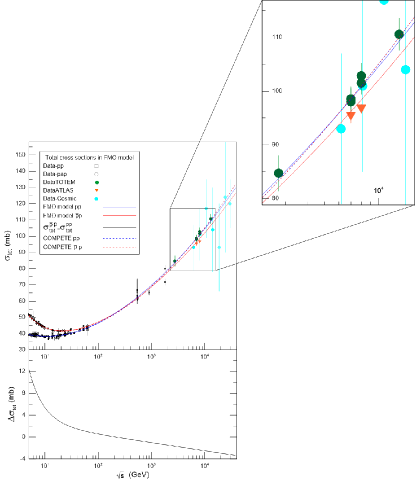
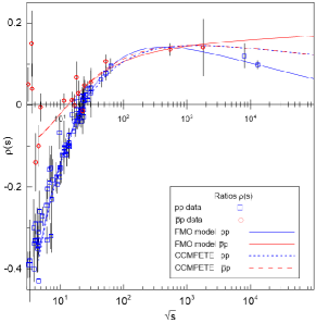
Figure 1: Total cross sections and ratios of the real to imaginary part of the forward elastic amplitude in FMO model (solid lines). The curves (dashed lines) of the best COMPETE fit COMPETE are shown also for a comparison

This study shows that, the new TOTEM datum $\rho_{pp}$ = 0.1$\pm$ 0.01 can be considered as the first certain experimental discovery of the Odderon, namely in its maximal form.

4.1.2 FMO model in a more general form at $t=0$

It is important to check if the Froissaron-Maximal Odderon (FMO) approach is the only model in agreement with the LHC data. We put the question: is the maximality of strong interactions not only in agreement with experimental data but it is even required by them? To find the answer on the question we have considered the generalized the FMO approach by relaxing the $\ln^{2}(s/s_{0})$ constraints both in the even-and odd-under-crossing amplitude MN-1 .

So, we considered the following form of the amplitudes:

$$F^{H}_{+}(z)=i(s-2m^{2})[H_{1}\ln^{\mu_{+}}(-iz)+H_{2}\ln^{\mu_{+}-1}(-iz)+H_{3}],$$ (33)

$$F^{MO}_{-}(z)=(s-2m^{2})[O_{1}\ln^{\mu_{-}}(-iz)+O_{2}\ln^{\mu_{-}-1}(-iz)+O_{3}],$$ (34)

$$F^{R}_{\pm}(z)\equiv\binom{P,R_{+}}{O,R_{-}}=-\binom{1}{i}C^{R}_{\pm}(-iz)^{\alpha_{\pm}(0)}.$$ (35)

For $\mu_{+}=\mu_{-}=2$ and $\alpha_{P}(0)=\alpha_{O}(0)=1$ we get exactly the FMO model of the ref. MN-0 . Our aim is verify which values of $\mu_{+}$ and $\mu_{-}$, as well as which values of $\alpha_{P}(0)$ and $\alpha_{O}(0)$ are the best for fitting all existing experimental data on $\sigma_{tot}(s)$ and $\rho(s)$.

The parameters $\mu_{+}$ and $\mu_{-}$ are not arbitrary. They are constrained by analyticity, unitarity, crossing-symmetry and positivity of cross sections (see Eqs. (9-11)).

The results of fitting are quite spectacular (see the details in MN-1 ): the values of $\mu_{+}$ and $\mu_{-}$ come back to the saturation values $\mu_{+}=2$ and $\mu_{-}=2$. Intercepts $\alpha_{P}(0)$ of Pomeron when it is free comes back to the value $\alpha_{P}(0)=1$. Thus we show that, in spite of a considerable freedom of a large class of amplitudes, the experimental data choose the maximal form of the FMO model, namely the maximal growth with energy of $\sigma_{tot}(s)$ and the maximal growth of the difference $|\sigma_{tot}^{pp}(s)-\sigma_{tot}^{\bar{p}p}(s)|$ Eden .

5 FMO and experimental data on $d\sigma(s,t)/dt$

The FMO model defined by Eqs. (25-30) was applied to describe simultaneously the $pp$ and $\bar{p}p$ total cross sections $\sigma_{t}^{pp}(s),\,\,\sigma_{t}^{\bar{p}p}$, ratios $\rho^{pp}(s),\,\,\rho^{\bar{p}p}(s)$ and differential cross sections $d\sigma^{pp}(s,t)/dt,\,\,d\sigma^{\bar{p}p}(s,t)/dt$ in the region of $s$ and $t$ described in the beginning of the Section 4.

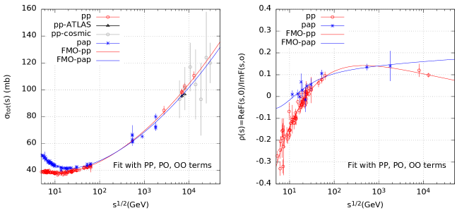
Figure 2: Total $pp$ and $\bar{p}p$ cross sections (left panel) and ratios $\rho^{pp}$ and $\rho^{\bar{p}p}$ (right panel) in the FMO model

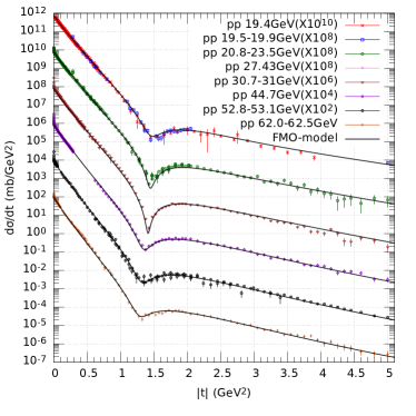
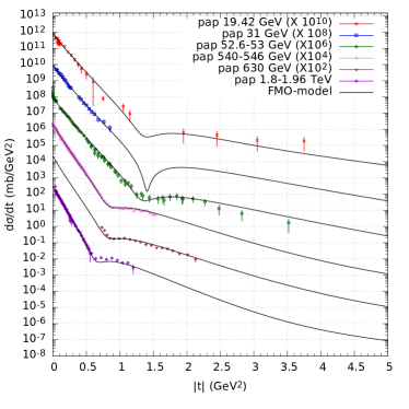
Figure 3: $pp$ (left panel) and $\bar{p}p$ (right panel) differential cross sections at 19 GeV $<\sqrt{s}<$ 2 TeV in FMO model

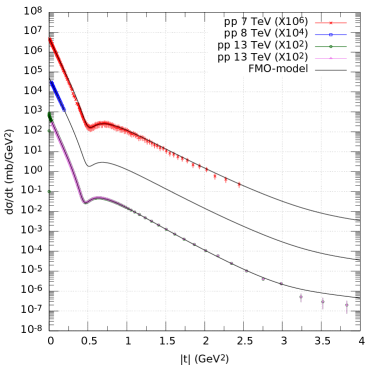
Figure 4: Differential $pp$ cross sections at LHC energies in FMO model

6 Conclusion

The TOTEM experiments firmly established the experimental existence of the Odderon, 45 years after its theoretical prediction. The Froissaron-Maximal Odderon (FMO) approach is the only existing model which describes the totality of experimental data (including the TOTEM results) in a wide range of energies and momentum transfers.

Acknowledgement The authors thank Prof. S. Giani, Prof. K. Osterberg, Prof. T. CsÃrgà and Dr. J. Kaspar for their very useful comments.

References

- (1) G. Antchev et al. ,CERN-EP-2017-321-V2, 2017; arXiv:1712.06153, [hep-ex].
- (2) G. Antchev et al., CERN-EP-2017-335, 2017.
- (3) J.R. Cudell et al., Phys.Rev.Lett. 89 (2002) 201801, 1.
- (4) R.F. Avila, P. Gauron, B. Nicolescu, Eur.Phys.J. C49 (2007) 581.
- (5) E. Martynov, B. Nicolescu, Phys. Lett., B778 (2018) 414.
- (6) E. Martynov, B. Nicolescu, Phys. Lett., B786 (2018) 207.
- (7) E. Martynov, B. Nicolescu, arXiv:1808.08580,[hep-ph].
- (8) R.J. Eden, Rev. Mod. Phys. 43 (1971) 15.
- (9) H. Cornille and A. Martin, Phys. Lett 40B (1972) 671.
- (10) G. Auberson, T. Kinoshita and A. Martin, Phys. Rev. D 3 (1971) 3185.
- (11) J.B. Bronzan, G.L. Kane, U.P. Sukhatme, Phys.Lett. 49B (1974) 272.
- (12) K. Kang, B. Nicolescu, Phys.Rev. D11 (1975) 2461.
- (13) G.F. Chew, Rev. Mod. Phys. 34 (1962) 394.
- (14) L. Łukazsuk, B. Nicolescu, Lett. al Nuovo Cimento 8 (1973), 405.
- (15) D. Joynson, E. Leader, B. Nicolescu, C. Lopez, IL Nuovo CIimento, 30A (1975) 345.
- (16) P. Gauron, L. Łukazsuk, B. Nicolescu, Physics Letters, B 294 (1992) 298.
- (17) E. Martynov, B. Nicolescu, ]Eur.Phys.J. C56 (2008) 57.
- (18) E. Martynov, Phys.Rev., D76 (2007) 074030, 1; Phys.Rev., D87 (2013) 40186, 1.
- (19) F. Nemes, Oral presentation at the 4th Elba Workshop on Forward Physics @ LHC Energy, Elba, Italy, 24-26 May, 2018. https://indico.cern.ch/event/705748/timetable/ .
- (20) F. Ravera, Oral presentation at the 134th LHCC Meeting, CERN, 30 May, 2018. https://indico.cern.ch/event/726320/ .