On-line parameter and state estimation of an air handling unit model: experimental results using the modulating function method

Abstract

This paper considers the on-line implementation of the modulating function method, for parameter and state estimation, for the model of an air-handling unit, central element of HVAC systems. After recalling the few elements of the method, more attention is paid on issues related to its on-line implementation, issues for which we use two different techniques. Experimental results are obtained after implementation of the algorithms on a heat flow experiment, and they are compared with conventional techniques (conventional tools from Matlab for parameter estimation, and a simple Luenberger observer for state estimation) for their validation.

1 Introduction

The challenges of the clear evidence of climate change [13] bring in the front-line new regulations which aim to reduce the green-house gas emissions in all sectors. A notable amount of emissions as well as energy consumption is accounted by buildings, both in the industrial and residential sector. According to [34] the need for heating is going to decrease while the cooling demand in buildings is going to increase in the coming decades due to the climate change. In this respect, heating ventilation and air conditioning (HVAC) systems with higher energy efficiency and better building designs are continuously researched and developed.

To facilitate the transition towards reducing the energy consumption and the green-house gas emissions, mathematical models of buildings have been intensively used. The simulation tools available today [10] and the ongoing research offer a high variety of possibilities when it comes to design optimization [21], renewable integration [41], retrofitting [14], on-line fault detection diagnosis [7] and even optimized real-time control.

The HVAC system is one very important part of the building, which in Europe is estimated to share $76\%$ of the total energy use [17]. The duty of this system is to ensure a comfortable indoor environment by regulating the temperature and the air quality. The well-functioning of the HVAC system will contribute also to an optimal energy consumption. Several subsystems are considered when modeling an HVAC system, as explained in [36]. Among them, the air handling unit (AHU) is the subsystem whose role is to condition the air circulated through the building. Different models have been proposed in the literature for modeling an AHU: physical models described by partial differential equations used by most of the simulation tools available [10], transfer functions [4], data-driven models [2], and hybrid models or reduced-order models (ROM) [3].

The latter lead to many possibilities as they easily link to estimation and control scenarios where real-time capabilities are important. In this paper, we investigate the use of the so-called modulating function method to perform both state and parameter estimation on a continuous-time ROM based on a simple thermal-electrical analogy [15]. In comparison with more conventional approaches using discrete-time such as Kalman filtering, performing both state and parameter estimation in continuous-time relates better to the formalism in which the system is originally modeled and ensures the convergence of the estimates to the real values when sampling time approaches zero [39]. Compared to their discrete-time counterparts estimating either parameters or state components is the necessity of considering time derivatives. The modulating function technique, originally introduced by Shinbrot [38], allows to circumvent this issue elegantly, with the use of fixed-length time integrals of the measured signals, akin continuous-time FIR filtering. This offers the additional advantages of giving estimates after a fixed and predetermined amount of time, contrary to usual Kalman-based filtering methods. Originally proposed towards parameter estimation, the modulating function method was more recently extended to include state estimation [23] [19].

Many studies considering the modulating function approach showed satisfactory performance, but mostly in simulations using artificial data [19] or sources generated from real profiles [5]. In contrast to that and to the best of our knowledge, not many applications can be found in the literature dealing with experiments done on actual measurements, to the notable exception of [11], where Hartley modulating functions are used to estimate the parameters of a thyristor driven DC-motor.

This paper addresses the question of real-time deterministic parameter and state estimation of an air handling unit using the modulating function method. The corresponding algorithms are implemented in Matlab/Simulink on an actual heat flow model and experimental results based on noisy measurements are presented. While the model itself is easy to develop and implement, performing estimation of its parameters and states is still a challenge given the actual distributed nature of these parameters, which are also subject to possible changes over time. In doing so, we also look at practical aspects related to implementation issues for using the modulating function method in an on-line situation, and which we believe has been less considered in the literature. Preliminary results were reported in [18].

After this introduction, we start this paper by briefly explaining the principle of an HVAC system and that of an AHU, and give a simple reduced-order model (ROM) of the latter (section 2). Then, the basics of the modulating function method are recalled for both parameter and the state estimation in a state-space context (section 3). A following section is more specifically addressed to issues that are more prone to arise in an on-line scenario, i.e. possible singularities coming from the choice of the modulating function, and ease of implementation of the moving-horizon version in a block diagram environment such as Simulink. For this, we use two different techniques, each one dedicated to these two specific issues (section 4). We validate the proposed techniques on a heat flow model and discuss our experimental results (section 5). Brief concluding remarks end this paper (section 6).

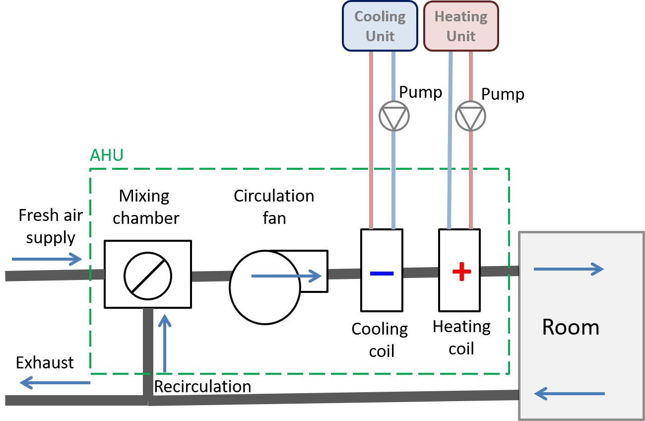
Figure 1: Air flow diagram through a typical fan coil compact HVAC

2 Heat Flow Model of an AHU

2.1 System description

The HVAC system within a building can be configured in many different ways with regards to the buildings’ layout and purpose, application or users’ needs. It usually contains a variety of components such as chillers, cooling towers, condensing boilers, AHUs, heat pumps, heat recovery units, fans, control valves, pipes, etc. as described, for example, in [36]. The air flow in a typical compact HVAC system can be represented by the schematic diagram shown in Fig. 1. The heating and cooling coils are part of separate networks with complex units that deliver cold or heat based on requirements. Similar representations can be seen in [12] or [8].

An important component of the HVAC system is the AHU (marked with green dashed box in Fig. 1). The role of this component is to condition the air that is used for the ventilation of the rooms in order to maintain a comfortable indoor environment in terms of temperature and air quality. In this unit, the fresh air is mixed with air coming from the rooms in a mixing chamber, then is circulated by a constant air volume flow fan over a cooling/heating coil. Based on the needs, the air is heated or cooled accordingly, so that the temperature at the exit of the unit achieves prescribed values.

2.2 Mathematical modeling

Many models have been developed to represent the dynamic heat flow behavior of an AHU. In the existing literature, the models that have been developed range from the use basic physics [37] to advanced data mining algorithms such as artificial neural networks and other machine learning techniques [1]. An overview of the variety of these models can be found in [4].

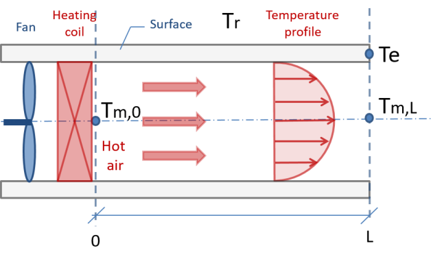
Figure 2: Internal heat flow profile

The heat flow which is considered here is schematically represented in Fig. 2. It simply consist of a fan, a heating coil, and a duct where temperature sensors can be placed. As expected from basic considerations, the temperature profile of the flowing medium, as well as the heat transfer coefficients typically varies with the length $L$ of the duct (see for example [6]). However, in the present application, only the temperature at the exit of the unit is of interest as it is typically the one which one wants to regulate. Hence we will, in the following, consider the measured temperature $T_{m,L}$, hereafter simply shortened as $T_{m}$. In order to model this heat flow, we resort to second-order linear ROM. A similar albeit first-order model is described in [3].

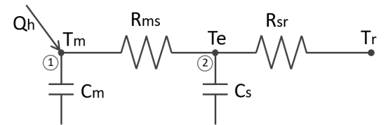
Figure 3: RC network analogy of the heat flow

The proposed 2-nd order linear model uses the resistance capacitor (RC) network analogy depicted in Fig. 3. In order to develop the model, we first write a flow balance equation for each node. Hence, we get

$$C_{m}\frac{dT_{m}}{dt}=\frac{1}{R_{ms}}(T_{e}-T_{m})+Q_{h}$$ (1)

for node 1, representing the air inside the unit, where $T_{m}$ is the measured temperature in the AHU and $T_{e}$ is the envelope/surface temperature of the AHU, while $Q_{h}$ is the heating/cooling load added in the AHU. The constant parameters of this flow balance equation are $C_{m}$, the summed heat capacity of the sensor and of the air inside the unit and $R_{ms}$, the thermal resistance between the temperature sensor and the envelope of the unit.
For node 2, the surface/envelope of the unit, we have the differential relation

$$C_{s}\frac{dT_{e}}{dt}=\frac{1}{R_{ms}}(T_{m}-T_{e})+\frac{1}{R_{sr}}(T_{r}-T_{e})\\$$ (2)

where $T_{r}$ is the temperature of the room surrounding the unit. In equation (2), constant parameters are $C_{s}$, the heat capacity of the envelope of the AHU, $R_{ms}$, the thermal resistance between the sensor and the surface of the unit, and $R_{sr}$, the total thermal resistance between the surface of the unit and the room.

From (1)-(2), it is simple to obtain the state-space representation

$$\dot{\mathbf{x}} =\mathbf{Ax}+\mathbf{Bu}$$ (3)

$$y =\mathbf{Cx}$$ (4)

where, defining the state vector and the input vector as

$$\mathbf{x}=\left[T_{m},T_{e}\right]^{T},$$ (5)

and

$$\mathbf{u}=\left[Q_{h},T_{r}\right]^{T}$$ (6)

while assuming we only measure the temperature at the end of the unit, i.e. $y=T_{m}$, we have the matrices

$$\mathbf{A}=\begin{bmatrix}-\frac{1}{C_{m}R_{ms}}&\frac{1}{C_{m}R_{ms}}\\ \frac{1}{C_{s}R_{ms}}&-(\frac{1}{C_{s}R_{ms}}+\frac{1}{C_{s}R_{sr}})\\ \end{bmatrix},$$ (7)

$$\mathbf{B}=\begin{bmatrix}\frac{1}{C_{m}}&0\\ 0&\frac{1}{C_{s}R_{sr}}\\ \end{bmatrix},$$ (8)

$$\mathbf{C}=\begin{bmatrix}1&0\end{bmatrix}.$$ (9)

3 The Modulating Function Method: parameter and state estimation

In this section, we briefly recall the basics of the modulating function method. For the sake of clarity, we do so on single-input single-output systems, with the multiple-input case as a direct extension.

The modulating function method being primarily based on an input-output description of a dynamical system, we start, as a preliminary by transforming our state-space presentation (3)-(4). Hence, considering the $n$-dimensional case where $\mathbf{x}\in\mathbb{R}^{n}$, $u\in\mathbb{R}$ and $y\in\mathbb{R}$, we differentiate the output equation (4) $n-1$ times and get the well-known expression

$$\bar{\mathbf{y}}=\mathbb{O}\mathbf{x}+\mathbf{T}\bar{\mathbf{u}}$$ (10)

where $\bar{\mathbf{y}}=[y,\dot{y},...,y^{(n-1)}]^{T}$ and $\bar{\mathbf{u}}=[u,\dot{u},...,u^{(n-1)}]^{T}$. Matrix $\mathbb{O}$ is the well-known observability matrix of the Kalman criterion and matrix $\mathbf{T}$ is the system specific Toeplitz matrix given by

$$\mathbf{T}=\begin{bmatrix}\mathbf{0}&\mathbf{0}&\ldots&\mathbf{0}\\ \mathbf{C}\mathbf{B}&\mathbf{0}&\ddots&\vdots\\ \vdots&\vdots&\ddots&\mathbf{0}\\ \mathbf{C}\mathbf{A}^{n-2}\mathbf{B}&\mathbf{C}\mathbf{A}^{n-3}\mathbf{B}&\dots&\mathbf{0}\\ \end{bmatrix}.$$ (11)

Then, differentiating equation (4) one more time and isolating $\mathbf{x}$ in expression (10), we get

$$y^{(n)}=\mathbf{C}\mathbf{A}^{n}\mathbb{O}^{-1}(\bar{\mathbf{y}}-\mathbf{T}\bar{\mathbf{u}})+\mathbf{C}\mathbb{C}^{R}\bar{\mathbf{u}}\\$$ (12)

where the reversed controllability matrix $\mathbb{C}^{R}$ is given by

$$\mathbb{C}^{R}=[\mathbf{A}^{(n-1)}\mathbf{B},\mathbf{A}^{(n-2)}\mathbf{B},...,\mathbf{A}\mathbf{B},\mathbf{B}].$$ (13)

Note that an obvious condition for expression (12) to be defined is the observability of state-space representation (3)-(4). We thus have the input-output form

$$y^{(n)}=-\mathbf{a}^{T}\bar{\mathbf{y}}+\mathbf{b}^{T}\bar{\mathbf{u}}$$ (14)

where $\mathbf{a}^{T}=\mathbf{C}\mathbf{A}^{n}\mathbb{O}^{-1}=[a_{0},a_{1},...,a_{n-1}]$ and $\mathbf{b}^{T}=\mathbf{C}\mathbb{C}^{R}-\mathbf{C}\mathbf{A}^{n}\mathbb{O}^{-1}\mathbf{T}=[b_{0},b_{1},...,b_{n-1}]$. Defining then the vector $\mathbf{Y}$ as $\mathbf{Y}=[\bar{\mathbf{y}}^{T},\bar{\mathbf{u}}^{T}]^{T}$, the following parametric form is obtained

$$y^{(n)}=\mathbf{Y}^{T}\bm{\uptheta},$$ (15)

where the unknown parameter vector $\bm{\uptheta}\in\mathbb{R}^{2n}$ is given by $\bm{\uptheta}=[-\mathbf{a}^{T},\mathbf{b}^{T}]^{T}$. In case a constant and unknown disturbance $d$ is impacting the system’s behavior at the same level as the input, expression (15) can be simply modified such that $\mathbf{Y}_{d}=[1,\mathbf{Y}^{T}]^{T}$ replaces $\mathbf{Y}$ and $\bm{\uptheta}_{d}=[d,\bm{\uptheta}^{T}]^{T}$ replaces $\bm{\uptheta}$.

Before proceeding, let us first recall the definition of a modulating function (see [23], [19]).

Definition 1.

The sufficiently smooth function $\varphi:[0,T]\rightarrow\mathbb{R}$ is called a modulating function (of order $k$) if at least one of its boundaries and its derivatives up to order $k$ equals zero, i.e. if

$$\varphi^{(i)}(0)\cdot\varphi^{(i)}(T)=0,i=\overline{0,k-1}.$$ (16)

A modulating function where $\varphi^{(i)}(0)=0$ and $\varphi^{(i)}(T)\neq 0$ (for $i=\overline{0,k-1}$) is called a left modulating function, while a modulating function with $\varphi^{(i)}(0)\neq 0$ and $\varphi^{(i)}(T)=0$ is called a right modulating function. If a modulating function is such that we have $\varphi^{(i)}(0)=\varphi^{(i)}(T)=0$, then it is called a total modulating function.

Note a more general definition of a modulating function (see [19]) allows to include expanding horizons, allowing thus to include alternative integral approaches [28] [35].

In this paper, we are interested in on-line estimation. Regarding parameter estimation, we hereby use the following receding-horizon integral operator on the signal $y(t)$, using a total modulating function given by [30]

$$L^{i}[y]:=\int_{t-T}^{t}(-1)^{i}\varphi^{(i)}(\tau-t+T)y(\tau)d\tau.$$ (17)

where $i=\overline{0,k-1}$ and $T>0$. Due to the fact that $\varphi(t)$ is a total modulating function and by simple integration by parts, operator (17) has the important property that

$$L^{0}[y^{(i)}]=L^{i}[y].$$ (18)

Then, applying operator $L^{0}[\cdot]$ on each time-varying signal of (15), and using property (18), we are able to avoid both explicit time-derivatives of measured signals and unknown initial conditions to get

$$z=\mathbf{w}^{T}\bm{\uptheta},$$ (19)

where

$$z=L^{n}[y]$$ (20)

and

$$\mathbf{w}=[L^{0}[y],L^{1}[y],...,L^{n-1}[y],L^{0}[u],L^{1}[u],...,L^{n-1}[u]]^{T}.$$ (21)

Finally, we can obtain an estimate of parameter vector $\bm{\uptheta}$ by either proceeding to a conventional receding-horizon Gramian-based estimator [32] [33] over a horizon $T^{\prime}>0$, or aggregate a sufficient number of expressions (19), each one obtained with a different total modulating function, so that with $m_{t}\geq 2n$ total modulating functions, we get the set of linear equations

$$\mathbf{z}=\mathbf{W}^{T}\bm{\uptheta}$$ (22)

where $\mathbf{z}=[z_{1},z_{2},...,z_{m_{t}}]^{T}$ and $\mathbf{W}=[\mathbf{w}_{1},\mathbf{w}_{2},...,\mathbf{w}_{m_{t}}]$. In this case, we can in principle directly get the parameter vector estimate by computing

$$\hat{\bm{\uptheta}}=\left(\mathbf{W}\mathbf{W}^{T}\right)^{-1}\mathbf{W}\mathbf{z}$$ (23)

or, alternatively, proceed by adding another receding-horizon stage similar to the Gramian-based estimator alluded to above in order to remove noise further, and define the estimate as

$$\hat{\bm{\uptheta}}=\left(\int_{t-T^{\prime}}^{t}\mathbf{W}(\tau)\mathbf{W}^{T}(\tau)d\tau\right)^{-1}\int_{t-T^{\prime}}^{t}\mathbf{W}(\tau)\mathbf{z}(\tau)d\tau.$$ (24)

Turning now to state estimation, we resort to an integral operator based, this time, on a left modulating function, and given by

$$L^{i}_{l}[y]:=\int_{t-T}^{t}(-1)^{i}\varphi_{l}^{(i)}(\tau-t+T)y(\tau)d\tau,$$ (25)

where $\varphi_{l}(t)\in[0,T]$ is a left modulating function. Because of the fact that $\varphi_{l}(T)\neq 0$, we have

$$L^{0}_{l}[y^{(i)}]=\sum_{k=0}^{i-1}(-1)^{k}\varphi_{l}^{(k)}(T)y^{(i-1-k)}(t)+L^{i}_{l}[y].$$ (26)

Proceeding then by applying operator $L^{0}_{l}[.]$ on each signal of (14), we get the expression

$$\bm{\upvarphi}_{l}\bar{\mathbf{y}}+\mathbf{a}^{T}\bm{\Gamma}_{l}\bar{\mathbf{y}}-\mathbf{b}^{T}\bm{\Gamma}_{l}\bar{\mathbf{u}}=\mathbf{b}^{T}\mathbf{L}_{l}[u]-\mathbf{a}^{T}\mathbf{L}_{l}[y]-L_{l}^{n}[y]$$ (27)

where

$$\bm{\upvarphi}_{l}=[(-1)^{n-1}\varphi_{l}^{(n-1)}(T),(-1)^{n-2}\varphi_{l}^{(n-2)}(T),\ldots,(-1)^{0}\varphi_{l}^{(0)}(T)],$$ (28)

$$\bm{\Gamma}_{l}\!=\!\mbox{$\begin{bmatrix}0&0&\cdots&0\\[1.72218pt] (-1)^{0}\varphi_{l}^{(0)}(T)&0&\ddots&\vdots\\[1.72218pt] \vdots&\ddots&\ddots&0\\[1.72218pt] (-1)^{n-2}\varphi_{l}^{(0)}(T)&\ldots&(-1)^{0}\varphi_{l}^{(0)}(T)&0\end{bmatrix}$}$$ (29)

and

$$\mathbf{L}_{l}[y]=\left[L^{0}_{l}[y],L^{1}_{l}[y],...,L^{n-1}_{l}[y]\right]^{T}$$ (30)

(and similarly for $\mathbf{L}_{l}[u]$).
Noticing then that

$$\left(\bm{\upvarphi}_{l}+\mathbf{a}^{T}\bm{\Gamma}_{l}\right)\mathbf{T}=\mathbf{b}^{T}\bm{\Gamma}_{l},$$ (31)

expression (27) can be put into a form similar to (19), i.e. we have

$$z_{l}=\mathbf{w}_{l}^{T}\left(\bar{\mathbf{y}}-\mathbf{T}\bar{\mathbf{u}}\right),$$ (32)

where

$$z_{l}=\mathbf{b}^{T}\mathbf{L}_{l}[u]-\mathbf{a}^{T}\mathbf{L}_{l}[y]-L_{l}^{n}[y]$$ (33)

and

$$\mathbf{w}_{l}=\left(\bm{\upvarphi}_{l}+\mathbf{a}^{T}\bm{\Gamma}_{l}\right)^{T}.$$ (34)

Combining then $m_{l}\geq n$ left modulating functions, we obtain, similarly to (22), the expression

$$\mathbf{z}_{l}=\mathbf{W}_{l}^{T}\left(\bar{\mathbf{y}}-\mathbf{T}\bar{\mathbf{u}}\right),$$ (35)

which, defining the state corresponding to an observability canonical form as

$$\bar{\mathbf{x}}=\bar{\mathbf{y}}-\mathbf{T}\bar{\mathbf{u}},$$ (36)

leads to its estimate $\hat{\bar{\mathbf{x}}}$ with an expression similar to (23). Alternatively, we can also estimate the original state of the system (3)-(4) by either using (10) or the simple transformation

$$\hat{\mathbf{x}}=\mathbb{O}^{-1}\hat{\bar{\mathbf{x}}}.$$ (37)

4 Implementing the modulating function method for on-line applications

4.1 Using time-varying modulating functions

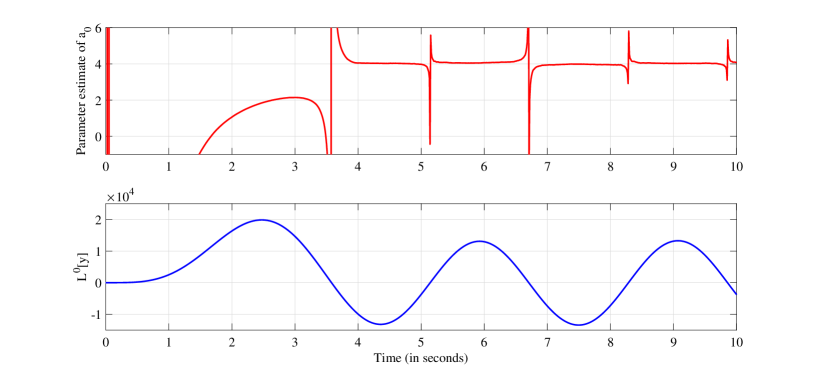
Figure 4: Parameter estimate $\hat{a}_{0}$ (top) and operator $L^{0}[y]$ (bottom) for the oscillator example (38).

Early works on the use of the modulating function method for offline identification of unknown parameters (see for example [31]) start with the definition of a set of specific and predefined modulating functions, which can take different forms (ie Hartly, splines, trigonometric functions, etc). Once a sufficient number of modulating functions are used, one can get a parameter estimate directly by simple inversion, as in (22). However, when considering an on-line and receding-horizon situation, this can generally lead, especially with the presence of noise on the measurements, to singularity issues. For example, considering the trivial system

$$\ddot{y}+a_{0}y=0,$$ (38)

applying the modulating function method would simply lead to

$$\hat{a}_{0}=-\frac{L^{2}[y]}{L^{0}[y]},$$ (39)

where the denominator of (39) could create difficulties. As an illustration, we have simulated the sinusoidal signal $y(t)=15\sin 2t$, corrupted with a uniform noise. As can be seen in Fig. 4, the estimate of $a_{0}$, obtained with the fixed total modulating function $\varphi(t)=t^{2}(t-T)^{2}$, shows singularities around the time when the signal $L^{0}[y](t)$ has its zero-crossings (see also similar spiking behaviors in Figure 3 of [9]). Seeing $L^{0}[y](t)=<\varphi,y>$ as a dot product between two functions, one has therefore an orthogonality issue between these functions.

While one way to go around this issue typically consists of using a gradient or recursive least-squares algorithm (or even using more modulating functions), another possibility is to continuously redefine the modulating functions based on the current batch of the measured signals $y(t)$ and $u(t)$.
Indeed, setting the number of total modulating functions to $m_{t}=2n$, we impose a normalizing constraint represented as

$$\mathbf{W}=\mathbf{I}_{m_{t}}\text{.}$$ (40)

In this way, we are simply bypassing the matrix inversion of (22) or (24). Realizing this constraint hence consists of finding the set of $m_{t}$ modulating functions that will fulfil (40). Since $\mathbf{W}$ is composed of $m_{t}$ vectors (21), where $L^{i}[y]$ is given by (17), we have a set of $m_{t}$ integro-differential equations, where the unknowns are the $m_{t}$ total modulating functions $\varphi_{k}$’s, which are also constrained at both their boundaries due to their total modulating function nature.

Let us then transform this set of integro-differential equations into integral equations by considering the $n$-th order derivative of $\varphi(t)$ arising in expression (20), and define the new function $\alpha:[0,T]\rightarrow\mathbb{R}$ as

$$\alpha(t):=\varphi^{(n)}(t).$$ (41)

Then, using the anti-derivative notation

$$f^{(-i)}(\tau):=\int_{0}^{\tau}\int_{0}^{\tau_{i}}...\int_{0}^{\tau_{2}}f(\tau_{1})d\tau_{1}\,d\tau_{2}\,\ldots\,d\tau_{i},$$ (42)

the right boundaries of the derivatives of a total modulating function $\varphi(t)$ can simply be re-written as

$$\alpha^{(-i)}(T)=0\hskip 14.22636pt,i=\overline{1,n}.$$ (43)

while the zero left boundary conditions are simply fulfilled thanks to the successive integration of $\alpha$. Thus, integral operator can now be re-written as

$$L^{i}[y]:=\int_{t-T}^{t}(-1)^{i}\alpha^{(i-n)}(\tau-t+T)y(\tau)d\tau,$$ (44)

so that $\mathbf{w}$ in (21) only consists of integrals of $\alpha$. Hence, expression (40) is now a set of integral equations. Grouping the right boundary conditions (43) similarly, we also get

$$\bm{\Gamma}=\mathbf{0}_{n\times m_{t}},$$ (45)

where $\bm{\Gamma}=[\bm{\upalpha}_{1},\bm{\upalpha}_{2},...,\bm{\upalpha}_{m_{t}}]$, with each vector $\bm{\upalpha}_{j}$ composed by all boundary conditions (43) for this specific modulating function, i.e. $\bm{\upalpha}_{j}=[\alpha_{j}^{(-n)},\alpha_{j}^{(-n+1)},...,\alpha_{j}^{(-1)}]^{T}$.
Combining finally (40) with (45), we have a system of linear integral equations, which is simple to solve numerically (details of this numerical method are given in Appendix A). Once a function $\alpha(\cdot)$ is obtained for each instant $t$, constraint (40) is fulfilled, and Gramian-like expression (24) is simply replaced with

$$\hat{\bm{\uptheta}}(t)=\frac{1}{T^{\prime}}\int_{t-T^{\prime}}^{t}{\mathbf{z}}(\tau)d\tau.$$ (46)

As for state estimation, it is also possible to normalize $\mathbf{W}_{l}$ similarly so that we have the state estimate

$$\hat{\mathbf{x}}=\mathbb{O}^{-1}\mathbf{z}_{l}.$$ (47)

The most notable difference with parameter estimation, is that, since $\mathbf{W}_{l}$ in (35) does not depend directly on the measured signals, the $m_{l}=n$ left modulating functions $\varphi_{l,j}(\cdot)$ can be chosen once and for all $t$. Note that a similar kind of normalization was also mentioned in the context of least-squares observers (see [29]).

4.2 Direct continuous-time implementation

When needing to choose a particular estimation method, one can obviously focus on performance in terms of the best possible match between the output of the considered plant and its corresponding predicted output using the parameter estimates. However, other factors can also be under consideration, such as ease of implementation, portability of the code, etc. Regarding the on-line use of modulating functions, the latter are usually first discretized (as they would be in the previous subsection or as in [9] and [30]). However, modern tools for simulation and control such as Matlab/Simulink allows one to program systems and algorithms directly in a continuous-time setting, thus allowing for the additional advantage of being able to consider non-regular samplings. In this section, we present one way to do that, with in mind direct continuous-time implementation, as opposed to looking primarly at performance.
To do so, we first begin by introducing a function $\psi:[0,T]\rightarrow\mathbb{R}$, which we will refer to as reversed modulating function, and where $\psi(\cdot)$ is such that

$$\psi(t):=\varphi(T-t)$$ (48)

where $\varphi(\cdot)$ is our usual modulating function of the very basic following definition 1. In this case, note that, because of reversal (48), a left reversed modulating function corresponds to a right modulating function, and vice-versa. Then, replace operator (17) with

$$M^{i}[y]:=\int_{t-T}^{t}\psi^{(i)}(t-\tau)y(\tau)d\tau.$$ (49)

The advantage of (49), is that, besides its slightly simpler expression than (17), it is directly put under a usual convolution form. Note, also similarly to (18), we have the property that $M^{0}[y^{(i)}]=M^{i}[y]$.
Next, we notice that many modulating functions defined in the literature can be expressed by the solution of a differential equation. For example, the total modulating function $\varphi(t)=t^{2}(t-T)^{2}$ used for example (38) is the solution of differential equation $\varphi^{(4)}(t)=0$. Hence, we introduce the following state-space representation

$$\dot{\bm{\chi}} =\mathbf{\Lambda}\bm{\chi},\,\,\,\bm{\chi}(0)=\mathbf{l}$$ (50)

$$\psi =\mathbf{\Sigma}\bm{\chi}$$ (51)

where the state vector $\bm{\chi}\in\mathbb{R}^{n_{\psi}}$.Thus, integral operator (49) can easily be rewritten using some advantages of state-space representations. For example, $M^{0}[y]$ can be rewritten as

$$M^{0}[y]=\int_{t-T}^{t}\mathbf{\Sigma}e^{\mathbf{\Lambda}(t-\tau)}\mathbf{l}\,y(\tau)d\tau.$$ (52)

and similarly for the other $M^{i}[y]$’s. Defining now the new vector $\bm{\xi}_{y}\in\mathbb{R}^{n_{\psi}}$ as

$$\bm{\xi}_{y}:=\int_{0}^{t}e^{\mathbf{\Lambda}(t-\tau)}\mathbf{l}\,y(\tau)d\tau,$$ (53)

then it can be shown that

$$M^{0}[y]=\mathbf{\Sigma}\left[\bm{\xi}_{y}(t)-e^{\mathbf{\Lambda}T}\bm{\xi}_{y}(t-T)\right]$$ (54)

where vector $\bm{\xi}_{y}(t)$ is obtained as the solution of differential equation

$$\dot{\bm{\xi}}_{y}=\mathbf{\Lambda}\bm{\xi}_{y}+\mathbf{l}y.$$ (55)

Interestingly, assuming now that system (50) is stable means that filter (55)-(54) can be used to implement $M^{0}[y]$ in software tools such as Matlab/Simulink without having to proceed to a preliminary discretization (the same is of course valid for $M^{0}[u]$, with a state vector $\bm{\xi}_{u}$). Note that computing $M^{i}[y]$ is not more difficult, and we would simply have

$$M^{i}[y]=\mathbf{\Sigma}\mathbf{\Lambda}^{i}\left[\bm{\xi}_{y}(t)-e^{\mathbf{\Lambda}T}\bm{\xi}_{y}(t-T)\right].$$ (56)

Gathering now the $M^{i}[y]$ terms similarly to (30), we have

$$\mathbf{M}[y]=\mathbb{O}_{MF}\left[\bm{\xi}_{y}(t)-e^{\mathbf{\Lambda}T}\bm{\xi}_{y}(t-T)\right],$$ (57)

where

$$\mathbf{M}[y]=\left[M^{0}[y],M^{1}[y],...,M^{n-1}[y]\right]^{T}$$ (58)

and

$$\mathbb{O}_{MF}=\left[\mathbf{\Sigma}^{T},(\mathbf{\Sigma\Lambda})^{T},...,(\mathbf{\Sigma\Lambda}^{n-1})^{T}\right]^{T}.$$ (59)

From there, we end up with regression (19) again, where

$$\mathbf{w}=\left[\mathbf{M}^{T}[y],\mathbf{M}^{T}[u]\right]^{T}$$ (60)

while $z$ is given by

$$z=M^{n}[y].$$ (61)

In case one wants to favor speed over precision, it is possible to use a single total (reversed) modulating function and use a Gramian-based expression in order to get the parameter estimate. Another advantage of using expressions such as (52) or (54), where the modulating function is generated by a stable system, is that similar expressions can also be used to obtain the parameter estimates themselves. Indeed, as in [32], we can use a generalized Gramian expression where the kernel is generated thanks to a reversed modulating function. Indeed, multiply each term of (19) by $\psi(t-\tau)\mathbf{w}(\tau)$ and integrate to get

$$\int_{t-T}^{t}\psi(t-\tau)\mathbf{w}(\tau)z(\tau)d\tau=\int_{t-T}^{t}\psi(t-\tau)\mathbf{w}(\tau)\mathbf{w}^{T}(\tau)d\tau\,\bm{\uptheta}$$ (62)

which can be rewritten as

$$M^{0}[\mathbf{h}]=M^{0}[\mathbf{G}]\bm{\uptheta}$$ (63)

where we have vector $\mathbf{h}=\mathbf{w}z$ and matrix $\mathbf{G}=\mathbf{w}\mathbf{w}^{T}$. Proceeding in the same manner as we did from expressions (49) to (57), we can define, for $M^{0}[\mathbf{h}]$, the filter equations

$$\dot{\bm{\xi}}_{\mathbf{h}} =\underline{\mathbf{\Lambda}}\bm{\xi}_{\mathbf{h}}+\underline{\mathbf{l}}\mathbf{h}$$ (64)

$$M^{0}[\mathbf{h}] =\underline{\mathbf{\Sigma}}\left[\bm{\xi}_{\mathbf{h}}(t)-e^{\underline{\mathbf{\Lambda}}T}\bm{\xi}_{\mathbf{h}}(t-T)\right]$$ (65)

where $\bm{\xi}_{\mathbf{h}}\in\mathbb{R}^{2nn_{\psi}}$, and where $\underline{\mathbf{\Lambda}}=\mathbf{\Lambda}\otimes\mathbf{I}_{2n}$, $\underline{\mathbf{l}}=\mathbf{l}\otimes\mathbf{I}_{2n}$ and $\underline{\mathbf{\Sigma}}=\mathbf{\Sigma}\otimes\mathbf{I}_{2n}$ (with $\otimes$ for the Kronecker symbol). For $M^{0}[\mathbf{G}]$, we have same kind of filter, this time with a matrix differential equation

$$\dot{\bm{\Xi}}_{\mathbf{G}} =\underline{\mathbf{\Lambda}}\bm{\Xi}_{\mathbf{G}}+\underline{\mathbf{l}}\mathbf{G}$$ (66)

$$M^{0}[\mathbf{G}] =\underline{\mathbf{\Sigma}}\left[\bm{\Xi}_{\mathbf{G}}(t)-e^{\underline{\mathbf{\Lambda}}T}\bm{\Xi}_{\mathbf{G}}(t-T)\right]$$ (67)

where $\bm{\Xi}_{\mathbf{G}}\in\mathbb{R}^{2nn_{\psi}\times 2n}$. Finally, an estimate of parameter vector $\bm{\uptheta}$ is obtained by simple inversion as

$$\hat{\bm{\uptheta}}=\left(M^{0}[\mathbf{G}]\right)^{-1}M^{0}[\mathbf{h}].$$ (68)

Interestingly, and moving now to state estimation, the method simply consists in repeating the steps (32) to (37) by taking into account that left modulating integral operators $L^{i}_{l}[y]$ and $L^{i}_{l}[u]$ are replaced by the right reversed modulating integral operators $M^{i}_{r}[y]$ and $M^{i}_{r}[u]$, where we have the property

$$M^{0}_{r}[y^{(i)}]=\sum_{k=0}^{i-1}\psi_{r}^{(k)}(0)y^{(i-1-k)}(t)+M^{i}_{r}[y]$$ (69)

(note, therefore, that steps (60) through (68) are obviously not necessary).

5 Case study

As a case study, a heat flow experimental chamber produced by Quanser company is considered. This plant reproduces the thermodynamics of an Air Handling Unit of an HVAC system. A few technical details related to the experimental set-up will be first introduced, while results of on-line parameter and state estimation and their validation will be presented afterwards.

5.1 Quanser heat flow chamber

The heat flow experiment (Fig. 5) consists of a fiber-glass chamber equipped with a fan blowing over an electric heating coil. Both the fan and the heater can be controlled externally with a $0-5V$ input signal. The air temperature inside the box is measured by three temperature sensors positioned equidistantly. Additionally, we make use of the Quanser Q8-USB Data Acquisition Board in order to enable the communication between the computer and the experimental chamber.

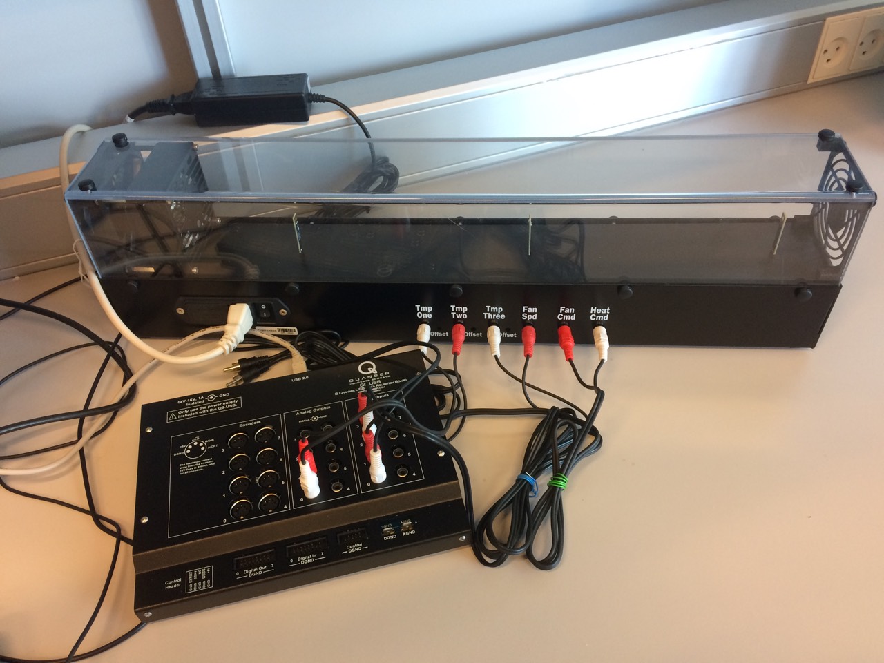
Figure 5: Quanser Heat Flow Experimental setup

5.2 Initial set-up and simulation environment

In the literature, the considered system model for control applications is usually of first order model (with or without time delay) [27][40]. However, in practice, a second-order model can have its importance, as the surface does not only represent the envelope/box storing heat but also other components (fans, dampers, filters). In a faulty situation where the box /components inside get overheated and can be damaged, estimating the box temperature can generate important information, and help in fault detection. The set-up will be used both for parameter estimation and state estimation scenarios where the latter uses the results of the former. Because the chamber is located in a closed indoor environment and the experiment is conducted on short time interval, we will assume that the room temperature ($T_{r}$) is unknown but constant during the experiment. In order to stay close to an actual operation of a constant flow AHU, the fan is operating with a constant speed during the whole experiment.

5.3 On-line parameter estimation

Using steps (10) to (15) on state-space representation (3)-(9), we obtain the ordinary differential equation

$$y^{(2)}=-a_{1}y^{(1)}-a_{0}y+b_{1}u^{(1)}+b_{0}u+d$$ (70)

where $y(t)=T_{m}(t)$ is the measured output, $u(t)$ is the input $Q_{h}$, and $a_{1}$, $a_{0}$, $b_{1}$, $b_{0}$ and $d$ are the unknown coefficients of the equation, the last one, $d$ representing the impact of the unknown input $T_{r}$ mentioned above, and considered here as a disturbance. These coefficients are related to the parameters of system (1)-(2) as follows:

$$a_{0}=\frac{1}{C_{m}R_{ms}C_{s}R_{sr}}$$ (71)

$$a_{1}=\frac{1}{C_{s}R_{ms}}+\frac{1}{C_{s}R_{sr}}+\frac{1}{C_{m}R_{ms}}$$ (72)

$$b_{0}=\frac{1}{C_{m}C_{s}R_{ms}}+\frac{1}{C_{m}C_{s}R_{sr}}$$ (73)

$$b_{1}=\frac{1}{C_{m}}$$ (74)

$$d=\frac{1}{C_{m}R_{ms}C_{s}R_{sr}}T_{r}$$ (75)

To perform the parameter estimation we have used the integration period $T=2000\ sec$ with a sampling time $T_{s}=2\ sec$, thus giving a total of $1000$ samples. The additional receding horizon interval for obtaining the estimates is $T^{\prime}=2000\ sec$.

Input profile and persistence of excitation

A key point in parameter estimation is the persistence of excitation of the input signal. Reliable estimates will be obtained if the input signal is sufficiently rich so that the observed response contains the required information to perform the estimation process. As specified in [24], if a specific matrix characteristic of the input signal is non-singular, the input is considered to be persistent. It is well-known that, when estimating the parameters of a system with an input signal having enough persistence of excitation, the estimated parameters approach their true values [20]. However, it is worth mentioning that, unfortunately, not enough attention has been given to the consideration of persistent inputs in building models and thus not many studies can be found on this topic [22].

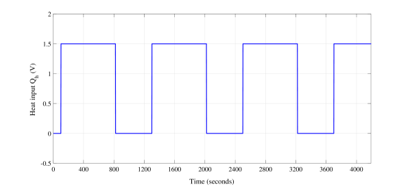
Figure 6: Input profile for parameter estimation

The considered input signal for parameter estimation is a pulse function shown in Fig. 6. This signal is informative enough to capture the dynamics of the heating chamber and obtain the estimates. The amplitude of signal is selected to $1.5V$ to change the temperature of chamber up to around $30^{\circ C}$. The period of the signal is $1200\ sec$ which is long enough for the plant to reach at least $80\%$ of its final value.

Estimates obtained using the modulating function

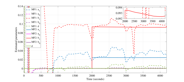
Figure 7: Estimated parameters

The results of parameter estimation using the modulating function method described in section 3 are presented in Fig. 7. The results are given for both methods: the time-vayring modulating function technique (continuous lines) and the direct continuous-time technique (dashed lines). As expected, the direct continuous-time technique, using only one modulating function, does not perform as well as the time-varying technique (although it is computationally more efficient). The latter shows quite good results and converges to an almost constant value after the additional receding horizon interval $T^{\prime}$.

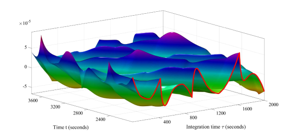
Figure 8: Evolution of the modulation function

Relating to the time-vayring modulating function method presented in section 4.1, Fig. 8 shows how one of the total modulating functions (corresponding in this case to $a_{1}$) evolves over time. The modulating function is a signal of length $T=2000sec$, and the figure shows its evolution from $t=2000$ to $t=3700$ (the curve highlighted in red is MF at time obtained $t=2000sec$). As it can be seen, the amplitude of the MF is constantly adapting to new incoming data/measurements that are fed on-line to the estimator.

5.4 Validation

Since there is no upfront knowledge about the real values of the parameters, we will compare the results of the modulating function method with the results of two well-known estimation methods available in the System Identification Toolbox for Matlab [25]. These two methods, applicable to continuous-time systems, are the Transfer Function method and the Grey-box estimation method. Moreover, for further validation of the results, the system output is reconstructed using the estimated parameters compared with the real measurements.

5.4.1 Continuous Transfer Function Estimation

The first method used for comparison is the “tfest” function of Matlab which estimates a continuous transfer function for the given data. In this method the input and output of the model are filtered using a pre-filter $L(s)$, and the differential equation of the system is written in a regression form with respect to the filtered signals. The parameters are then estimated to minimize the prediction error.

Matlab uses different numerical search methods to estimate the parameters iteratively. In case of selecting the default setting, a combination of four line search algorithms ’Subspace Gauss-Newton least squares search’, ’Levenberg-Marquardt least squares search’, ’Adaptive subspace Gauss-Newton search’, and ’Steepest descent least squares search’ methods will be applied and the first descent direction leading to a reduction in estimation cost is used.

In order to initialize the parameters, different algorithms are available in Matlab. The algorithm used in this study is the instrument variable approach in which the parameters are estimated using the least-squares method [16] and [26].

5.4.2 Grey-Box Model Estimation

The second method used for comparison is the grey-box model estimation using the “idgrey” function of Matlab. This method directly uses the parametric state-space representation of the system given in (3)-(4) and minimizes the prediction error.
Matlab uses the same numerical search methods as explained in section 5.4.1. However, contrary to the transfer function estimation technique, the initial value for the parameters should be given by the user.

Table 1: Summary of estimated parameters

	Grey-box	Transfer      Function	Modulating Function
$a_{0}$	1.2312e-06	1.454e-05	9.958e-6
$a_{1}$	0.0258	0.02447	0.02449
$b_{0}$	4.1891e-05	7.385e-05	6.81e-5
$b_{1}$	0.098591	0.09188	0.09236
$d$	1.2312e-06	3.3891e-04	2.1770e-04

Table 1 shows the estimated parameters using the MF method together with those obtained by the transfer function and grey-box approaches. As it can be seen, the results of the MF method are very close to the results of the transfer function method, while there is a discrepancy in some parameters with when compared to the grey-box method. The comparison is more clear in Fig. 9 where the output of the estimated models are plotted together and compared with the measured data. The goodness of the fit is $96.95\%$, $96.51\%$ and $97.42\%$, for the modulating function, transfer function and gray-box methods, respectively, which confirms the validity of the proposed MF method.

The main reason for achieving a slightly different (better) result by grey-box estimation method is that the reported goodness of fit was based on non-filtered measured data which matches the structure of grey-box method. The grey-box method works on the original input-output signals whereas the other two methods, i.e. modulating function and transfer function methods, use a pre-filter for the input-output signals ($L(s)$ in transfer function method and the modulating integral operators in the MF method). Therefore the optimization algorithm in the MF and transfer function methods minimizes the filtered error while the reported goodness of fit was based on the original error. In case we would define the goodness of fit based on filtered signals, a higher fit would be achieved for MF and transfer function methods.

Another important point that should be mentioned is that our implementation of the MF method is on-line while the other two methods are iterative and off-line. In particular, the convergence of the grey-box method highly depends on the initial guess for the parameters (in this study, the estimated parameters from MF method are considered as initial guess for the grey-box method). Therefore, achieving a result in the order of off-line methods in finite time further attests the acceptable performance of our results.

     

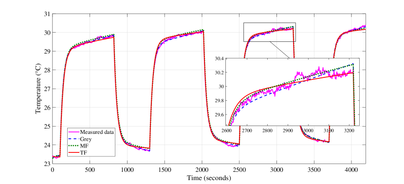
Figure 9: Validation - measured vs. simulated model output

5.5 On-line state estimation

Given the estimated parameters from previous section, it is straightforward to apply the method described in section 3 to obtain the state estimates. Here, both $T_{m}$ and $T_{s}$ are estimated on-line using an integration interval $T=50sec$ with sampling period $T_{s}=1sec$.

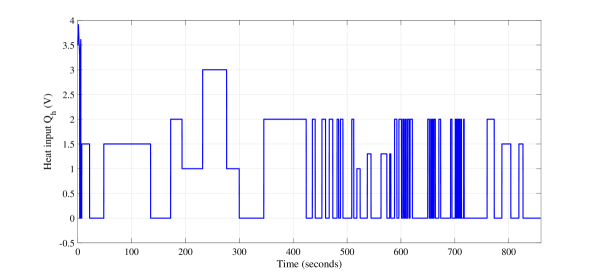
Figure 10: Input profile for state estimation

In a normal operation set-up, the requirements for the temperature at the exit of the AHU might not vary too much in a short time interval. However, to test the proposed state estimation algorithm in different work conditions, a pseudo random input profile shown in Fig. 10 is applied to the system. This is not a common operating profile, but it helps to visualize the state estimator and evaluate its behavior.

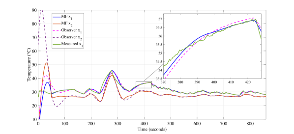
Figure 11: Measured vs. estimated temperature inside the heating chamber using the modulating function and simple observer.

In Fig. 11, it can be observed that the estimated temperature inside the chamber is very close to the noisy measured temperature. Also, as expected, the value for the state representing the envelope temperature of the chamber is lower than the temperature inside, and follows the same heating profile which is in perfect concordance with the heating input profile. The estimated states are comparably good with the ones obtained from a standard observer. In this specific case, the convergence of the states is faster due to the fixed integration interval, which ensures convergence after the first receding horizon window.

6 Conclusion

A 2nd order model is presented in this paper to represent the heat flow in the air handling unit present in compact HVAC systems. To facilitate the real-time applications of the model we have proposed an unconventional method, the modulating function, with two different implementation approaches.

As a case study, a heat flow experiment by Quanser, whose thermodynamics are very close to those of an AHU, is considered. The on-line parameter and state estimation algorithms were implemented in Matlab/Simulink. The results underline the potential of this approach, showing a good match between the measured and estimated parameters and states. A good convergence of the parameters was observed having as a baseline the parameters estimated with standard estimation methods: the transfer function method and the grey-box method. Moreover, using several (as opposed to only one) modulating functions gives a better estimation of the parameters compared with an approach that uses only one, at the cost of speed although the latter one mentioned requires less resources to implement and run. The method can be successfully used for on-line state estimation as well, the results being comparable good with a standard observer.

Appendix A - Numerical integration

For implementing the proposed estimation method a simple Riemann sum is used, taking into account that the signals $y(t)$ and $\mathbf{u}(t)$ are in practice sampled at regular intervals. Therefore, for the simple boundary condition (43), with $i=1$, we use the approximation

$$\alpha^{(-1)}(T)=\int_{t-T}^{t}\alpha(\tau-t+T)\,d\tau\approx\displaystyle\sum_{k=1}^{N}T_{s}\underline{\upalpha}(k)=T_{s}{\mathbf{1}}^{T}\underline{\bm{\upalpha}}$$ (76)

where $N$ is the number of samples over the interval, $T_{s}$ is the sampling period, and $\underline{\upalpha}(k)$ is the sampled value of function $\alpha$ at iteration $k$, which gives the vector $\underline{\bm{\upalpha}}^{T}=[\underline{\upalpha}(1),\underline{\upalpha}(2),...,\underline{\upalpha}(N+1)]^{T}$. Vector ${\mathbf{1}}$ is a vector of dimension $N$ containing only ones. Using a similar reasoning, $\alpha^{(-1)}(\tau)$ can be approximated as

$$\alpha^{(-1)}(\tau)=\int_{t-T}^{\tau}\alpha(\sigma-t+T)d\sigma\approx\displaystyle\sum_{l=1}^{k}T_{s}\underline{{\upalpha}}(l)=:\underline{{\upalpha}}^{(-1)}(k)$$ (77)

so that

$$\underline{\bm{\upalpha}}^{(-1)}=T_{s}\mathbf{Q}\underline{\bm{\upalpha}}$$ (78)

where $\underline{\bm{\upalpha}}^{(-1)T}=[\underline{{\upalpha}}^{(-1)}(1),\underline{{\upalpha}}^{(-1)}(2),...,\underline{{\upalpha}}^{(-1)}(N+1)]^{T}$, while the matrix $\mathbf{Q}$ is a lower triangular matrix of ones given by

$$\mathbf{Q}=\begin{bmatrix}1&0&\dots&0\\ \vdots&\ddots&\ddots&\vdots\\ 1&\dots&1&0\\ 1&1&\dots&1\\ \end{bmatrix}.$$ (79)

Hence, for $i=2$, condition (43) gives

$$\alpha^{(-2)}(T)=\int_{t-T}^{t}\alpha^{(-1)}(\tau-t+T)\,d\tau\approx T_{s}^{2}{\mathbf{1}}^{T}\mathbf{Q}\underline{\bm{\upalpha}}.$$ (80)

and for $i=\overline{3,n}$:

$$\alpha^{(-i)}(T)=\int_{t-T}^{t}\alpha^{(-i+1)}(\tau-t+T)\,d\tau\approx T_{s}^{i}{\mathbf{1}}^{T}\mathbf{Q}^{i-1}\underline{\bm{\upalpha}}.$$ (81)

The operators $L^{i}[y]$ of $\mathbf{w}$ in (44) can be similarly approximated, so that

$$\begin{split}L^{i}[y]:=\int_{t-T}^{t}(-1)^{i}\alpha^{(i-n)}(\tau-t+T)y(\tau)d\tau\\ \approx(-1)^{i}T_{s}^{n-i+1}\underline{{\mathbf{y}}}^{T}\mathbf{Q}^{n-i}\underline{\bm{\upalpha}},i=\overline{0,n-1}\end{split}$$ (82)

Likewise are defined the remaining terms of $\mathbf{w}$ in (44), where vector $\underline{{\mathbf{y}}}$ in (82) is replaced by $\underline{{\mathbf{u}}}$. Taking now $m_{t}=2n$ modulating functions, $\mathbf{W}$ in (40) can thus be approximated by

$$\mathbf{W}\approx\underline{\mathbf{W}}=\underline{\mathbf{K}}\,\underline{\underline{\upalpha}}$$ (83)

where $\underline{\underline{\bm{\upalpha}}}=[\underline{{\bm{\upalpha}}}_{1},\underline{{\bm{\upalpha}}}_{2},...,\underline{{\bm{\upalpha}}}_{m_{t}}]$ and the matrix $\underline{\mathbf{K}}$ is given by

$$\underline{\mathbf{K}}=\begin{bmatrix}(-1)^{0}T_{s}^{n+1}\underline{{\mathbf{y}}}^{T}\mathbf{Q}^{n}\\ \vdots\\ (-1)^{n-1}T_{s}^{2}\underline{{\mathbf{y}}}^{T}\mathbf{Q}\\ (-1)^{0}T_{s}^{n+1}\underline{{\mathbf{u}}}^{T}\mathbf{Q}^{n}\\ \vdots\\ (-1)^{n-1}T_{s}^{2}\underline{{\mathbf{u}}}^{T}\mathbf{Q}\\ \end{bmatrix}.$$ (84)

Proceeding similarly with the discrete approximation of $\mathbf{\Gamma}$ in (45), it can be expressed

$$\mathbf{\Gamma}\approx\underline{\mathbf{\Gamma}}=\underline{\mathbf{B}}\,\underline{\underline{\upalpha}}$$ (85)

where

$$\underline{\mathbf{B}}=\begin{bmatrix}T_{s}^{n}{\mathbf{1}}^{T}\mathbf{Q}^{n-1}\\ \vdots\\ T_{s}^{2}{\mathbf{1}}^{T}\mathbf{Q}\\ T_{s}{\mathbf{1}}^{T}\end{bmatrix}.$$ (86)

Then, matrix $\underline{\underline{\bm{\upalpha}}}$ is obtained by simple pseudoinversion, i.e.

$$\underline{\underline{\bm{\upalpha}}}=\begin{bmatrix}\underline{\mathbf{K}}\\ \underline{\mathbf{B}}\end{bmatrix}^{+}\begin{bmatrix}\mathbf{I}_{m_{\phi}}\\ \mathbf{0}_{n\times m_{\phi}}\end{bmatrix}.$$ (87)

The discrete approximation of $\mathbf{z}$ is given by

$$\mathbf{z}\approx\underline{\mathbf{z}}=T_{s}\underline{{\mathbf{y}}}^{T}\underline{\underline{\bm{\upalpha}}}.$$ (88)

The parameter estimate vector is finally obtained after applying the simple discretized version of receding-horizon expression (46).

References

- [1] A. Afram, A. S. Fung, F. Janabi-Sharifi, and K. Raahemifar, “Development and performance comparison of low-order black-box models for a residential hvac system,” Journal of Building Engineering, vol. 15, pp. 137–155, 2018.
- [2] A. Afram and F. Janabi-Sharifi, “Review of modeling methods for hvac systems,” Applied Thermal Engineering, vol. 67, no. 1-2, pp. 507–519, 2014.
- [3] ——, “Gray-box modeling and validation of residential hvac system for control system design,” Applied Energy, vol. 137, pp. 134–150, 2015.
- [4] Z. Afroz, G. Shafiullah, T. Urmee, and G. Higgins, “Modeling techniques used in building hvac control systems: A review,” Renewable and Sustainable Energy Reviews, 2017.
- [5] S. Asiri, S. Elmetennani, and T.-M. Laleg-Kirati, “Moving-horizon modulating functions-based algorithm for online source estimation in a first-order hyperbolic partial differential equation,” Journal of Solar Energy Engineering, vol. 139, no. 6, p. 061007, 2017.
- [6] T. L. Bergman and F. P. Incropera, Fundamentals of heat and mass transfer. John Wiley & Sons, 2011.
- [7] M. Bonvini, M. D. Sohn, J. Granderson, M. Wetter, and M. A. Piette, “Robust on-line fault detection diagnosis for hvac components based on nonlinear state estimation techniques,” Applied Energy, vol. 124, pp. 156 – 166, 2014. [Online]. Available: http://www.sciencedirect.com/science/article/pii/S0306261914002311
- [8] Y. Chen and S. Treado, “Development of a simulation platform based on dynamic models for hvac control analysis,” Energy and Buildings, vol. 68, pp. 376–386, 2014.
- [9] T. B. Co and S. Ungarala, “Batch scheme recursive parameter estimation of continuous-time systems using the modulating functions method,” Automatica, vol. 33, no. 6, pp. 1185–1191, 1997.
- [10] D. B. Crawley, J. W. Hand, M. Kummert, and B. T. Griffith, “Contrasting the capabilities of building energy performance simulation programs,” Building and Environment, vol. 43, no. 4, pp. 661 – 673, 2008, part Special: Building Performance Simulation.
- [11] S. Daniel-Berhe and H. Unbehauen, “Experimental physical parameter estimation of a thyristor driven dc-motor using the hmf-method,” Control Engineering Practice, vol. 6, no. 5, pp. 615–626, 1998.
- [12] D. Dey and B. Dong, “A probabilistic approach to diagnose faults of air handling units in buildings,” Energy and Buildings, vol. 130, pp. 177 – 187, 2016.
- [13] O. Edenhofer and K. Seyboth, “Intergovernmental panel on climate change (ipcc),” in Encyclopedia of Energy, Natural Resource, and Environmental Economics, J. F. Shogren, Ed. Waltham: Elsevier, 2013, pp. 48 – 56. [Online]. Available: http://www.sciencedirect.com/science/article/pii/B9780123750679001285
- [14] Y. Fan and X. Xia, “Building retrofit optimization models using notch test data considering energy performance certificate compliance,” Applied Energy, vol. 228, pp. 2140 – 2152, 2018. [Online]. Available: http://www.sciencedirect.com/science/article/pii/S0306261918310729
- [15] G. Fraisse, C. Viardot, O. Lafabrie, and G. Achard, “Development of a simplified and accurate building model based on electrical analogy,” Energy and buildings, vol. 34, no. 10, pp. 1017–1031, 2002.
- [16] H. Garnier, M. Mensler, and A. Richard, “Continuous-time model identification from sampled data: implementation issues and performance evaluation,” International journal of Control, vol. 76, no. 13, pp. 1337–1357, 2003.
- [17] M. Gruber, A. Trüschel, and J.-O. Dalenbäck, “Alternative strategies for supply air temperature control in office buildings,” Energy and Buildings, vol. 82, pp. 406–415, 2014.
- [18] A. Ionesi and J. Jouffroy, “On-line parameter estimation of an air handling unit model: experimental results using the modulating function method,” in 2018 IEEE International Conference on Advanced Intelligent Mechatronics (AIM), July 2018.
- [19] J. Jouffroy and J. Reger, “Finite-time simultaneous parameter and state estimation using modulating functions,” in Control Applications (CCA), 2015 IEEE Conference on. IEEE, 2015, pp. 394–399.
- [20] H. K. Khalil, “Adaptive output feedback control of nonlinear systems represented by input-output models,” IEEE Transactions on Automatic Control, vol. 41, no. 2, pp. 177–188, Feb 1996.
- [21] F. Kheiri, “A review on optimization methods applied in energy-efficient building geometry and envelope design,” Renewable and Sustainable Energy Reviews, vol. 92, pp. 897 – 920, 2018. [Online]. Available: http://www.sciencedirect.com/science/article/pii/S1364032118302624
- [22] X. Li and J. Wen, “Review of building energy modeling for control and operation,” Renewable and Sustainable Energy Reviews, vol. 37, pp. 517–537, 2014.
- [23] D.-Y. Liu, T.-M. Laleg-Kirati, W. Perruquetti, and O. Gibaru, “Non-asymptotic state estimation for a class of linear time-varying systems with unknown inputs,” in the 19th World Congress of the International Federation of Automatic Control 2014, 2014.
- [24] L. Ljung, Ed., System Identification (2Nd Ed.): Theory for the User. Upper Saddle River, NJ, USA: Prentice Hall PTR, 1999.
- [25] L. Ljung, “System identification toolbox for use with MATLAB,” 2007.
- [26] ——, Experiments with identification of continuous time models. Linköping University Electronic Press, 2009.
- [27] H. Malek, Y. Luo, and Y. Chen, “Identification and tuning fractional order proportional integral controllers for time delayed systems with a fractional pole,” Mechatronics, vol. 23, no. 7, pp. 746 – 754, 2013, 1. Fractional Order Modeling and Control in Mechatronics 2. Design, control, and software implementation for distributed MEMS (dMEMS).
- [28] A. Mathew and F. Fairman, “Identification in the presence of initial conditions,” IEEE Transactions on Automatic Control, vol. 17, no. 3, pp. 394–396, 1972.
- [29] A. Medvedev, “Continuous least-squares observers with applications,” IEEE Transactions on Automatic Control, vol. 41, no. 10, pp. 1530–1537, Oct 1996.
- [30] M. Noack, T. Botha, H. A. Hamersma, V. Ivanov, J. Reger, and S. Els, “Road profile estimation with modulation function based sensor fusion and series expansion for input reconstruction,” in Advanced Motion Control (AMC), 2018 IEEE 15th International Workshop on. IEEE, 2018, pp. 547–552.
- [31] A. Pearson and F. Lee, “On the identification of polynomial input-output differential systems,” IEEE Transactions on Automatic Control, vol. 30, no. 8, pp. 778–782, 1985.
- [32] J. Reger and J. Jouffroy, “On algebraic time-derivative estimation and deadbeat state reconstruction,” in Proceedings of the 48h IEEE Conference on Decision and Control (CDC) held jointly with 2009 28th Chinese Control Conference, Dec 2009, pp. 1740–1745.
- [33] ——, “Algebraische ableitungsschätzung im kontext der rekonstruierbarkeit (algebraic time-derivative estimation in the context of reconstructibility),” at-Automatisierungstechnik, vol. 56, no. 6 (2008), pp. 324–331, 2008.
- [34] J. M. Rey-Hernández, C. Yousif, D. Gatt, E. Velasco-Gómez, J. S. José-Alonso, and F. J. Rey-Martínez, “Modelling the long-term effect of climate change on a zero energy and carbon dioxide building through energy efficiency and renewables,” Energy and Buildings, vol. 174, pp. 85 – 96, 2018. [Online]. Available: http://www.sciencedirect.com/science/article/pii/S0378778817335764
- [35] D. C. SAHA and G. P. RAO, “Identification of lumped linear systems in the presence of unknown initial conditions via poisson moment functionals,” International Journal of Control, vol. 31, no. 4, pp. 637–644, 1980.
- [36] H. Satyavada and S. Baldi, “An integrated control-oriented modelling for hvac performance benchmarking,” Journal of Building Engineering, vol. 6, pp. 262–273, 2016.
- [37] H. Setayesh, H. Moradi, and A. Alasty, “A comparison between the minimum-order & full-order observers in robust control of the air handling units in the presence of uncertainty,” Energy and Buildings, vol. 91, pp. 115–130, 2015.
- [38] M. Shinbrot, “On the analysis of linear and nonlinear systems,” Trans. ASME, vol. 79, no. 3, pp. 547–552, 1957.
- [39] H. Unbehauen and P. Rao, “Identification of continuous-time systems: a tutorial,” IFAC Proceedings Volumes, vol. 30, no. 11, pp. 973–999, 1997.
- [40] K. Yamada, “Modified pid controllers for minimum phase systems and their practical application,” in Proceedings of The, 2005, pp. 457–460.
- [41] Y. Zhou, “Evaluation of renewable energy utilization efficiency in buildings with exergy analysis,” Applied Thermal Engineering, vol. 137, pp. 430 – 439, 2018. [Online]. Available: http://www.sciencedirect.com/science/article/pii/S1359431117362361