An Application of Global ILC Algorithm over Large Angular Scales to Estimate CMB Posterior Using Gibbs Sampling

Abstract

In this work, we formalize a new technique to investigate joint posterior density of Cosmic Microwave Background (CMB) signal and its theoretical angular power spectrum given the observed data, using the global internal-linear-combination (ILC) method first proposed by Sudevan & Saha (2017). We implement the method on low resolution CMB maps observed by WMAP and Planck satellite missions, using Gibbs sampling, assuming that the detector noise is negligible on large angular scales of the sky. The main products of our analysis are best fit CMB cleaned map and its theoretical angular power spectrum along with their error estimates. We validate the methodology by performing Monte Carlo simulations that includes realistic foreground models and noise levels consistent with WMAP and Planck observations. Our method has an unique advantage that the posterior density is obtained without any need to explicitly model foreground components. Secondly, the power spectrum results with the error estimates can be directly used for cosmological parameter estimations.

1. Introduction

Since the discovery of Cosmic Microwave Background (CMB) (Penzias & Wilson, 1965) rapid advancements in the field of its observation made it possible to map the primordial signal over the entire sky with increasingly higher resolution (Smoot et al., 1991; Bennett et al., 2013; Planck Collaboration et al., 2018b). Accurate measurement of temperature (and polarization) anisotropy of CMB, which arguably forms one of the cornerstones of the precision era of modern precision cosmology, provides us with a wealth of knowledge regarding the geometry, composition and the origin of the Universe (e.g., see Planck Collaboration et al. (2018a) and references therein). However, the observed CMB signal in the microwave region is strongly contaminated due to foreground emissions due to different astrophysical sources present within and outside our galaxy. Hence the challenge is to accurately recover the CMB signal for cosmological analysis, by minimizing contributions from various foregrounds emissions.

For reliable estimation of cosmological parameters, a desirable property of a CMB reconstruction method is that it produces both, the best guesses for the signal and its angular power spectrum along with their corresponding error (and bias, if any) estimates. Eriksen et al. (2004b, 2007, 2008a, 2008b); Planck Collaboration et al. (2016a, c) propose and implement a Gibbs sampling (Geman & Geman, 1984) approach to jointly estimate the CMB map, its angular power spectrum and all foreground components along with their error estimates using WMAP (Hinshaw et al., 2013) and Planck (Planck Collaboration et al., 2018b) observations. Eriksen et al. (2006); Gold et al. (2011) use a maximum likelihood approach to reconstruct simultaneously CMB and foreground components using prior information about CMB and detector noise covariance matrices and foreground models. Although, these methods are extremely useful for simultaneous reconstruction of CMB and all foreground components, an alternative approach for CMB reconstruction alone, is the so-called internal-linear-combination (ILC) method (Tegmark & Efstathiou, 1996; Tegmark et al., 2003; Bennett et al., 2003; Eriksen et al., 2004a; Saha et al., 2006) which does not rely upon any explicit model of foreground spectrum. In recent years the method has been investigated extensively. Saha et al. (2006) use this method to estimate CMB cross-power spectra by removing detector noise bias using WMAP maps. These authors also report presence of a possible negative bias at the low multipoles. Saha et al. (2008), for the first time, perform a rigorous analytical study of negative bias at the low multipoles for a single iteration ILC foreground removal procedure in harmonic space. Later Sudevan et al. (2017) find and correct a foreground leakage in iterative ILC algorithm in harmonic space by applying their technique on high resolution Planck and WMAP observations. Sudevan & Saha (2017) propose a global ILC method in pixel space by taking into account prior information of CMB covariance matrix under the assumption that detector noise can be ignored over the large angular scales of the sky. The method considerably improves the usual ILC method at low resolution, where no prior information about the CMB covariance is used. In spite of these progresses, a joint analysis of CMB signal and its angular power spectrum posterior density in a foreground model independent manner has not yet been explored in the literatures. The current article is aimed to provide a mechanism exactly to solve this problem. By estimating the posterior density of CMB signal and CMB theoretical angular power spectrum given the observed data over the large angular scales of the sky using the ILC method similar to Sudevan & Saha (2017), we provide the best fit estimates of both, CMB map and theoretical angular power spectrum along with their confidence interval regions. In the current article, we replace the CMB signal reconstruction technique by a faster harmonic domain algorithm than the pixel-space algorithm of Sudevan & Saha (2017). We use Gibbs sampling method (Gelman & Rubin, 1992) to draw samples from the joint conditional density. There are two important advantages of our method. First, the theoretical power spectrum results can directly be integrated to cosmological parameter estimation process. Second, the CMB posterior estimation can be achieved without any need to explicitly model the foreground components. The results, therefore, can not be sensitive to, foreground modeling uncertainties.

The early work of CMB component reconstruction is performed by Bennett et al. (1992) using a variant of ILC algorithm where prior information of free-free spectral index is used. Bunn et al. (1994); Bouchet et al. (1999) developed a Weiner filter approach. Basak & Delabrouille (2012, 2013) propose an ILC algorithm in needlet space, which can take into account local variation of foreground spectral properties both in the pixel and needlet space. Saha & Aluri (2016) use the ILC method to jointly reconstruct CMB Stokes Q polarization signal and other foreground components in presence of spatially varying spectral properties of polarized synchrotron emission using simulated observations of WMAP. In an interesting application of ILC method Saha (2011) and Purkayastha & Saha (2017) reconstruct CMB maps using Gaussian nature of CMB and non-Gaussian nature of astrophysical foregrounds.

In Section 2 we discuss the basic formalism. We describe the posterior estimation method in Section 3. In Section 4 we present the results of analysis of WMAP and Planck frequency maps at low resolution. We discuss convergence tests of the Gibbs chains in Section 5. We validate the posterior density estimation method by performing detailed Monte Carlo simulations using realistic foreground and detector noise model consistent with WMAP and Planck observations in Section 7. Finally, we conclude in Section 7.

2. Formalism

2.1. Data Model

Let us assume that, we have observations of foreground contaminated CMB maps at $n$ different frequencies. Without sacrificing any generality, we assume that, each of these maps has the same beam (and pixel) resolutions . The observed data set, ${\bf D}$, can be represented as ${\bf D}=\{{\bf X}_{1},{\bf X}_{2},...,{\bf X}_{n}\}$, where $\textbf{X}_{i}$, $i\in\{1,2,...,n\}$, is an $N\times 1$ column vector denoting the input foreground contaminated CMB map (in thermodynamic temperature unit) at a frequency $\nu_{i}$. $N$ represents the number of pixels in each input frequency map and ${\bf D}$ is an $N\times n$ matrix. Assuming detector noise is negligible  we have

$${\bf X}_{i}={\bf S}+{\bf F}_{i}\,,$$ (1)

where ${\bf S}$ is an $N\times 1$ column vector, representing the CMB signal  and ${\bf F}_{i}$ denotes a map of same size representing net foreground contamination at the frequency $\nu_{i}$.

2.2. CMB Posterior and Gibbs Sampling

The CMB posterior density is denoted as $P({\bf S},C_{\ell}|{\bf D})$, the joint density of CMB map, ${\bf S}$, and theoretical CMB angular power spectrum, $C_{\ell}$, given the observed data, ${\bf D}$.  A convenient way to establish the posterior density, without any need to evaluate it, is by drawing samples from the distribution itself. An useful sampling method in this context is the so called Gibbs sampling approach (Gelman & Rubin, 1992), which states that the posterior joint density under consideration conditioned on data can be established by following few steps.

1. Draw a sample, ${\bf S}^{i+1}$, from from conditional density of CMB signal ${\bf S}$ given both, the data ${\bf D}$ and some chosen CMB theoretical angular power spectrum, $C^{i}_{\ell}$. Symbolically,

   $${\bf S}^{i+1}\leftarrow P_{1}({\bf S}|{\bf D},C^{i}_{\ell})\,.$$ (2)

2. Now draw a sample of $C^{i+1}_{\ell}$ from the conditional density of $C_{\ell}$ given both, ${\bf D}$ and ${\bf S}^{i+1}$, which was obtained in the first step above. In symbols,

   $$C^{i+1}_{\ell}\leftarrow P_{2}(C_{\ell}|{\bf D},{\bf S}^{i})\,.$$ (3)

   At this stage one has a pair of samples ${\bf S}^{i+1},C^{i+1}_{\ell}$.

3. Repeat above two basic steps for $i=1$ to $\mathcal{N}$, where $\mathcal{N}$ is a large number, by replacing first $C^{i}_{\ell}$ by $C^{i+1}_{\ell}$ in step 1 above, and then replacing ${\bf S}^{i+1}$ in Eqn. 3 by the one obtained in Eqn. 2.

After some initial pair of samples of signal and theoretical power spectrum are discarded (i.e., after initial burn-in period has completed) they represent the desired samples drawn from the posterior density, $P({\bf S},C_{\ell}|{\bf D})$, under consideration.

2.3. Density of pure CMB signal

The probability density function of pure CMB signal ${\bf S}$ given a theoretical CMB angular power spectrum $C_{\ell}$ is given by,

$$P_{3}({\bf S}|C_{\ell})=\frac{1}{\sqrt{2^{r}\lambda_{1}\lambda_{2}...\lambda_{r}}}\exp{\left[-\frac{1}{2}{\bf S}^{T}{\bf C}^{\dagger}{\bf S}\right]}\,,$$ (4)

where ${\bf C}$ denotes the $N\times N$ pixel-pixel CMB covariance matrix of ${\bf S}$ at the chosen beam and pixel resolution. As discussed in Sudevan & Saha (2017), and as is the case in current article, rank $r$ of ${\bf C}$ is less than its size $N$, implying ${\bf C}$ is a singular matrix. ${\bf C}^{\dagger}$, therefore, represents the Moore-Penrose generalized inverse (Moore, 1920; Penrose, 1955) of ${\bf C}$. The element of ${\bf C}$ can be computed from the knowledge of the CMB theoretical angular power spectrum using Eqn. 6 of Sudevan & Saha (2017), by assuming that CMB map is statistically isotropic. The set of $\lambda_{k},k\in\{1,2,...,r\}$ in the denominator of Eqn. 4 represent the non-zero eigen values of ${\bf C}$.

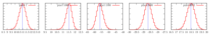
Figure 1.— The normalized probability density of CMB pixel temperatures for some selected pixels are shown in red. The normalization for each density is such that the peak corresponds to a value of unity. The horizontal axes represent pixel temperatures in the unit of $\mu K$ (thermodynamic). The positions of mean temperatures are shown by the blue vertical lines.

2.4. Drawing Samples of ${\bf S}$

How do we draw samples of ${\bf S}$ given ${\bf D}$ and $C_{\ell}$? We must do this without knowing or sampling the foreground components, to keep our method foreground model independent. This will be possible if we could somehow remove all foregrounds without using their model, given ${\bf D}$ and $C_{\ell}$. The cleaned map obtained by using the global ILC method described in Sudevan & Saha (2017) can be used exactly for this purpose, if we assume that, the detector noise is negligible and one has sufficient number of input frequency maps to remove all foreground components, as discussed in the current section. Let us consider the cleaned map, ${\bf Y}$, obtained by using linear combination of $n$ frequency maps $\{{\bf X}_{i}\}$,

$${\bf Y}=\sum_{i=1}^{n}w_{i}{\bf X}_{i}\,,$$ (5)

where $w_{i}$ represents the weight corresponding to the $i^{th}$ input frequency map. Clearly, we can neglect any detector noise contribution in ${\bf Y}$ since ${\bf X}_{i}$ themselves are assumed to contain negligible detector noise (e.g., see Eqn. 1). Since CMB follows blackbody distribution, to preserve the CMB signal in the cleaned map, the weights for all frequency maps are constrained to add to unity, i.e, $w_{1}+w_{2}+w_{3}+...+w_{n}=1$. Minimizing the CMB covariance weighted variance $\sigma^{2}={\bf Y}^{T}{\bf C}^{\dagger}{\bf Y}$ of the cleaned map ${\bf Y}$, subject to the above constraint on weights, as in Sudevan & Saha (2017), we obtain,

$${\bf W}=\frac{{\hat{\bf A}}^{\dagger}{\bf e}}{{\bf e}^{T}{\hat{\bf A}}^{\dagger}{\bf e}}\,,$$ (6)

where ${\bf W}$ is an $n\times 1$ column vector with the $i^{th}$ element given by the weight factor $w_{i}$. ${\bf e}$ denotes an $n\times 1$ column vector with all entries equal to unity, representing the frequency shape vector of the CMB component. Finally, the $(i,j)$ element of matrix ${\hat{\bf A}}$ can be computed in pixel-domain following,

$$\hat{A}_{ij}={\bf X}_{i}^{T}{\bf C}^{\dagger}{\bf X}_{j}\,.$$ (7)

However, computing above in pixel-space is a numerically expensive process. One can considerably simply Eqn. 7 in harmonic space. As shown in Appendix A, Eqn. 7 can conveniently be expressed in the multipole space following,

$$\hat{A}_{ij}=\sum_{\ell=2}^{\ell_{max}}\left(2\ell+1\right)\frac{\hat{\sigma}^{ij}_{\ell}}{C^{\prime}_{\ell}}\,,$$ (8)

where, $C^{\prime}_{\ell}$ represents the beam and pixel smoothed CMB theoretical power spectrum, $C^{\prime}_{\ell}=C_{\ell}B^{2}_{\ell}P^{2}_{\ell}$, $B_{\ell}$ and $P_{\ell}$ being the beam and pixel window functions respectively, and $\hat{\sigma}^{ij}_{\ell}$ represents the cross angular power spectrum between frequency maps ${\bf X}_{i}$ and ${\bf X}_{j}$ .

We assume that, there are $n_{f}$ different foreground components, each with a constant spectral index all over the sky . We denote the shape vector of $k^{th}$ foreground component by ${\bf f}_{k}$ (with $k\in\{1,2,...,n_{f}\}$) , each one of which is an $n\times 1$ column vector. Using Eqns. 1 and 6 in Eqn. 5 we obtain,

$${\bf Y}={\bf S}+\left[{\bf W}^{T}\sum_{k=1}^{n_{f}}{\bf f}_{k}\right]{\bf F}^{0}_{k}\,,$$ (9)

where ${\bf F}^{0}_{k}$ is an $N\times 1$ column vector representing an appropriately chosen template for the $k$ foreground component. Eqn. 9 shows that the cleaned maps contains the pure CMB signal plus some foreground residual given by the second term. To find these residuals, introducing matrix notation, we first write Eqn. 8 as

$${\hat{\bf A}}=\sum_{\ell=2}^{\ell_{max}}\frac{\left(2\ell+1\right)}{C^{\prime}_{\ell}}{\hat{\boldsymbol{\Sigma}}}_{\ell}\,,$$ (10)

where $n\times n$ data covariance matrix, $\hat{\boldsymbol{\Sigma}}_{\ell}$, in the harmonic space can be written in terms of CMB angular power spectrum, $\hat{C}_{\ell}$, of the particular random realization under consideration and the foreground covariance matrix ${\bf C}^{f}_{\ell}$, as,

$$\hat{\boldsymbol{\Sigma}}_{\ell}=\left[{\bf ee}^{T}\hat{C}_{\ell}+{\bf C}^{f}_{\ell}\right]B^{2}_{\ell}P^{2}_{\ell}\,.$$ (11)

Using Eqn. 11 and 10 in Eqn. 6 and following a procedure similar to Saha & Aluri (2016) we obtain,

$${\bf W}=\frac{\left({\bf I}-{{{\bf C}_{f}}}{{{\bf C}_{f}}}^{\dagger}\right){\bf{e}}}{{\bf e}^{T}\left({\bf I}-{{{\bf C}_{f}}}{{{\bf C}_{f}}}^{\dagger}\right){\bf{e}}}\,,$$ (12)

where ${\bf I}$ denotes the $n\times n$ identity matrix and

$${\bf C}_{f}=\sum_{\ell=2}^{\ell_{max}}\frac{\left(2\ell+1\right)}{C_{\ell}}{\bf C}^{f}_{\ell}\,,$$ (13)

The product ${\bf C}_{f}{\bf C}^{\dagger}_{f}$ represents the projector on the column space, $\mathcal{C}({\bf C}^{f})$, of ${\bf C}_{f}$. If we assume that $n_{f}<n$, which may be achieved by using sufficiently large number of input frequency maps, the null space of ${\bf C}_{f}$ is an non-empty set and ${\bf I}-{\bf C}_{f}{\bf C}^{\dagger}_{f}$ is a projector on this null space. Since, the shape vector, ${\bf f}_{k}$ of each foreground components with constant spectral indices completely lies on $\mathcal{C}({\bf C}_{f})$ we must have, ${\bf W}^{T}{\bf f}_{k}=0$, for all $k$. Therefore, from Eqn. 9 one finds that the foreground contamination in the final cleaned map at each pixel due to all foreground components disappears. Hence ${\bf Y}={\bf S}$.

Based upon preceding discussions, to sample ${\bf S}$ from $P_{1}({\bf S}|C_{\ell},{\bf D})$ we use Eqn. 5. The cleaned map in this case has the probability density as given by Eqn. 4 with the same covariance structure mentioned therein.

2.5. Drawing Samples of $C_{\ell}$

As discussed in Appendix B the conditional density $P_{2}(C_{\ell}|{\bf S},{\bf D})$ can be written as,

$$P_{2}\left(C_{\ell}|\hat{C}_{\ell}\right)\propto\left(\frac{1}{C_{\ell}}\right)^{\left(2\ell+1\right)/2}\exp\left[-\frac{\hat{C}_{\ell}\left(2\ell+1\right)}{2C_{\ell}}\right]\,,$$ (14)

where the variable $z={\hat{C}_{\ell}\left(2\ell+1\right)}/{C_{\ell}}$ follows a $\chi^{2}$ distribution of $2\ell-1$ degree of freedom. To draw samples of $C_{\ell}$ from Eqn. 14 we first draw $z$ from the $\chi^{2}$ distribution of $2\ell-1$ degrees of freedom, which is achieved by drawing $2\ell-1$ independent standard normal deviates and forming the sum of their squares. Given the value of $\hat{C}_{\ell}$ estimated from the map, we then find $C_{\ell}$ following $C_{\ell}={\hat{C}_{\ell}\left(2\ell+1\right)}/z$.

3. Methodology

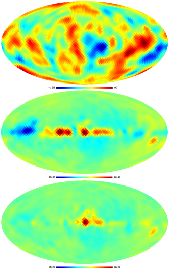
Figure 2.— Top panel shows the best-fit CMB map obtained by our method. The middle and bottom panels show the difference of our map from the Commander and NILC cleaned maps respectively. There is a noticeable similarity between the best-fit and NILC cleaned maps as seen from the bottom panel.

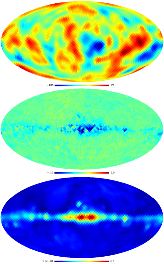
Figure 3.— Top panel shows the mean CMB map estimated by using all the cleaned maps obtained from the Gibbs samples. The mean map matches very well with the best-fit map shown in the top panel of Fig. 2. The middle panel show the difference between the best fit and the mean CMB maps. The bottom panel shows the standard deviation map obtained by using all the cleaned maps.

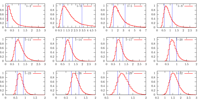
Figure 4.— Normalized densities of the CMB theoretical angular power spectrum obtained by Gibbs sampling for different multipoles. The horizontal axis for each sub plot represents $\ell\left(\ell+1\right)C_{\ell}/(2\pi)$ in the unit $1000$ $\mu K^{2}$. The region within the two vertical lines represent $1-\sigma$ confidence interval for the theoretical angular power spectrum.

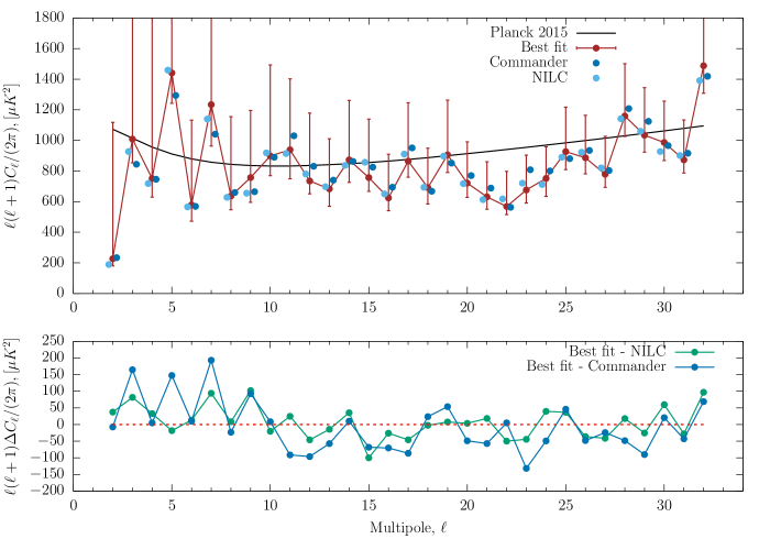
Figure 5.— Top panel shows the best-fit CMB theoretical angular power spectrum along with the asymmetric error bars indicating $68.27\%$ confidence intervals obtained from the Gibbs samples in brown line. The sky blue points represent the angular power spectrum estimated from NILC CMB map. The deep blue points represent the same estimated from the Commander CMB maps. (For visual purpose, both these spectra are shifted along the horizontal axis slightly from the actual positions of the integer multipoles.) The black line shows the Planck 2015 theoretical power spectrum as a guide to eye. The bottom panel shows a zoomed in version of the differences of Commander and NILC angular power spectra respectively from the best-fit angular power spectrum of top panel.

We use WMAP nine-year $10$ difference assembly (DA) maps and seven Planck 2015 maps, three of the later are at LFI frequencies ($30$, $40$ and $70$ GHz) and the rest at four HFI frequencies ($100,143,217$ and $353$ GHz). The processing of input maps remains identical to Sudevan & Saha (2017) and results in a total of $12$ input maps, five at WMAP and seven at Planck frequencies. We note that, since we are interested in analysis over large angular scales of the sky, where detector noise can be ignored, we chose a low pixel resolution defined by HEALPix  parameter $N_{side}$ = $16$ and a Gaussian beam smoothing of $9^{\circ}$ FWHM for each input map. We remove both monopole and dipole from all the full sky input maps before the analysis. To sample the posterior density $P({\bf S},C_{\ell}|{\bf D})$ we simulate a total of $10$ Gibbs chains, each containing $5000$ joint samples of cleaned maps and theoretical power spectrum, following the three sampling steps described in Section 2. At any given chain and at any given iteration, to sample ${\bf S}$ we use Eqn. 5, where the weights are described by the vector ${\bf W}$ defined by Eqn. 6. The elements of matrix ${\bf A}$ that appears in 6 are computed following Eqn. 8 using the last sampled $C_{\ell}$ values. After sampling ${\bf S}$ we estimate its full sky power spectrum , $\hat{C}_{\ell}$, which we use to obtain a new sample of $C_{\ell}$ using the method described in Section 2.5. We emphasize that both $\hat{C}_{\ell}$ and $C_{\ell}$ contain beam and pixel smoothing effects absorbed in them. We note in passing, that the weights as given by Eqn. 6 are however insensitive to such smoothing since in Eqn. 8, both $C_{\ell}$ and $\hat{\sigma}^{ij}_{\ell}$ contain same smoothing effects. The initial choice of $C_{\ell}$ for each chain is made by drawing them uniformly within $\pm 3\Delta C_{\ell}$ around the Planck best-fit theoretical power spectrum (Planck Collaboration et al., 2016d), where $\Delta C_{\ell}$ denotes error due to cosmic variance alone.

All $10$ chains generates a total of $50000$ joint samples of cleaned map and theoretical CMB power spectrum. The burn in phase in each chain is very brief. Visually, this phase does not appear to contain more than a few Gibbs iterations. We, however, remove $50$ initial Gibbs iterations from each chain as a conservative estimate of burn-in period. After the burn-in rejection we have a total of $49500$ samples from all chains.

4. Results

4.1. Cleaned Maps

Using all samples after burn in rejection we estimate the marginalized probability density of CMB temperature at each pixel given the observed data. The normalized probability densities obtained by division by the corresponding mode of the marginalized density function for some selected pixels over the sky are shown in Fig. 1. These density functions are approximately symmetric with some visible asymmetry near the tails. The positions of mean temperatures are shown by the blue vertical lines for each pixel of this plot. We estimate the best-fit CMB cleaned map by taking the pixel temperatures corresponding to the location of mode of density for each pixel at $N_{side}=16$. We show the best-fit map at the top panel of Fig. 2. We compare the best-fit map with other CMB cleaned maps which are obtained by using different methods by other science groups. We show the differences of best fit map from Planck Commander and NILC (needlet space ILC) cleaned maps (Planck Collaboration et al., 2016b) respectively at the middle and bottom panels of the same figure at $9^{\circ}$ Gaussian beam resolution. Clearly, our best-fit map matches well with the Commander cleaned map with some minor differences along the galactic plane, which is expected to contain some foreground residuals in any foreground removal method. It is worth to emphasize the striking similarity between the best-fit and NILC CMB map. Interestingly, the best-fit map contains somewhat lower pixel temperatures at isolated locations along the galactic plane than the Commander or NILC map.

From Fig. 1 we see that the mean and marginalized posterior maximum of CMB temperature at different pixels agree closely with each other. We estimate the mean CMB map using all $49500$ samples for each pixel and show this at the top panel of Fig. 3. The mean map matches very well with the best-fit CMB map shown in top panel of the Fig. 2. We have plotted the difference between the best fit and mean map in the bottom panel of Fig. 3. Both the maps agree with each other within an absolute difference of $1\mu K$. In order to quantify the reconstruction error in the cleaned CMB map obtained after each iteration of Gibbs sampling, we generate a standard deviation map using all $49500$ cleaned maps. We show this map at the bottom panel of Fig. 3. From this panel we see that the reconstruction error is very small all over the sky. The maximum reconstruction error is visible along the galactic plane and towards the center of our galaxy where the input frequency maps contain strong foreground contaminations.

4.2. Angular Power Spectrum

We estimate the marginalized probability density of CMB theoretical angular power spectrum and show the results in Fig. 4 for different multipoles. Like the density functions of the pixel temperatures as discussed in Section 4.1, we normalize these densities to a value of unity at their peaks. The horizontal axis of each plot of this figure represents $\ell\left(\ell+1\right)C_{\ell}/(2\pi)$ in the unit of $1000$ $\mu K^{2}$. The density functions show long asymmetric tails for low multipoles (e.g., $\ell=2,3,5$). For large multipoles ($\ell\geq 20$) the asymmetry of the densities become gradually reduced. The region within the two vertical lines in each plot show $1-\sigma$ ($68.27\%$) confidence interval for the CMB theoretical power spectrum for the corresponding multipole.

In top panel of Fig. 5 we show the best-fit theoretical CMB angular power spectrum in brown color, defined by the positions of peaks of marginalized angular power spectrum density functions (e.g., Fig 4). The asymmetric error bars at each $\ell$ show the $1-\sigma$ confidence interval for the theoretical angular power spectrum. The black line shows the theoretical power spectrum consistent with Planck 2015 results (Planck Collaboration et al., 2016d). The best-fit theoretical angular power spectrum agree well with the spectra estimated from Commander and NILC cleaned maps, which are shown by green and blue points respectively.In the bottom panel of Fig. 5 we show the difference of the best fit and Commander (or NILC) power spectrum. Our best fit theoretical power spectrum agrees very well with the spectrum estimated from the NILC CMB map.

5. Convergence Tests

Each of the Gibbs sampling chains for the estimation of CMB signal and its theoretical angular power spectrum joint posterior consists of $4950$ sampling after rejection of burn-in phase. A diagnosis is necessary to be certain that these samples have converged to the actual targeted CMB posterior - a condition when satisfied inference drawn about any parameter by using the chains, does not depend upon the initial point where the chain starts. Gelman & Rubin (1992) propose that lack of any such convergence is better diagnosed if we simulate a set of ‘parallel’ chains than a single chain. Using all the $10$ Gibbs chains we, therefore, check for convergence by using the Gelman-Rubin statistic Gelman & Rubin (1992). Detailed description of the statistic is given in Gelman & Rubin (1992); Brooks & Gelman (1998), however, for completeness we define the statistic below.

Let us assume that we have generated $M$ number of different chains and let $L$ be the number of steps in each chain after rejection of samples during the burn-in period . For a model parameter $\theta$, let us assume that the sample posterior mean is given by $\bar{\theta}_{m}$ for $m^{th}$ chain using all $L$ samples. Let corresponding sample posterior variance is $\bar{\sigma}^{2}_{m}$. Then the between-chain ($B/L$) and within-chain variances ($W$) are respectively given by,

$$B = \frac{L}{M-1}\sum_{m=1}^{M}\big{(}\bar{\theta}_{m}-\bar{\theta}\big{)}^{2}$$ (15)

$$W = \frac{1}{M}\sum_{m=1}^{M}\bar{\sigma}^{2}_{m}\,,$$ (16)

where $\bar{\theta}$ is the overall posterior mean of the samples estimated from all $M$ chains and is given by $\bar{\theta}=\frac{1}{M}\sum_{m=1}^{M}\theta_{m}$. We define the pooled posterior variance following,

$$\hat{V}=\frac{L-1}{L}W+\frac{M+1}{ML}B\,,$$ (17)

which can be used to compute the Gelman-Rubin statistic $R$ as follows,

$$R=\sqrt{\frac{\hat{V}}{W}}\,.$$ (18)

Following Gelman & Rubin (1992); Brooks & Gelman (1998) a value of $R$ close to unity implies that each of $M$ Gibbs chains have converged to the target posterior density.

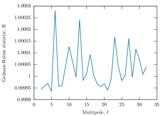
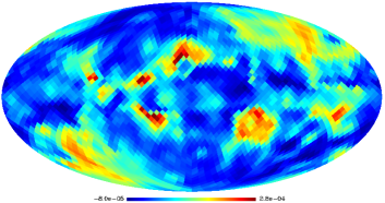
Figure 6.— Top panel shows Gelman-Rubin statistic, $R$ estimated for all the multipoles of this work. The bottom panel shows map of $R-1$ for all pixels. Close values of $R$ to unity in both cases indicate convergence is achieved in all the Gibbs chains.

We have plotted the Gelman-Rubin statistic, $R$, for the theoretical angular power spectrum samples for the multipole range $2\leq\ell\leq 32$ in top panel of Fig. 6. The value of $R$ lies well within $0.9999$ and $1.0003$ implying convergence. In the bottom panel of Fig. 6 we show the map of $R-1$ all over the sky. $R$ lies with in $0.99992$ and $1.0002$ for all the pixels implying again convergence of the Gibbs chains.

6. Monte Carlo Simulations

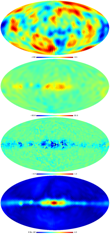
Figure 7.— Top panel shows the best-fit cleaned CMB map obtained from Monte Carlo simulations. The second panel shows the difference between the best-fit and the input CMB map used in the simulation. The third panel shows the difference between the best-fit and mean CMB map. The last panel shows the standard deviation map.

We generate a set of input maps at the $12$ different WMAP and Planck frequencies at a Gaussian beam resolution $9^{\circ}$ and $N_{side}=16$ following the same procedure as described in Sudevan & Saha (2017). We do not reproduce the methodology in the article and refer to the above article for a description about the input frequency maps. We note that, in the current work, we need to simulate only one random realization of the $12$ input frequency maps. The random CMB realization used in the input frequency maps is generated using the CMB theoretical angular power spectrum consistent with Planck 2015 results. As is the case for our analysis on the Planck and WMAP observations, we remove both monopole and dipole from all the simulated input maps before sampling from the posterior density $P({\bf S},C_{\ell}|{\bf D})$. We simulate a total of $10$ Gibbs chains. To draw the first cleaned map sample we initialize the theoretical CMB power spectrum uniformly within $\pm 3\Delta_{\ell}$ of the true theoretical spectrum, where $\Delta_{\ell}$ represents cosmic variance induced error. As in the case of analysis of WMAP and Plank observed maps, for simulations also we find that the burn-in period ends very rapidly. In particular, from the trace plots of pixel temperature of the cleaned maps we see that burn-in phase completes within a few samples. As a conservative approach, however, we reject initial $50$ samples from each Gibbs chain. After, burn-in rejection we have a set of $4950$ joint samples of cleaned map and theoretical angular power spectrum from each Gibbs chain.

Using all cleaned map samples from all chains after burn-in rejection we form a marginalized density of the CMB temperature at each $N_{side}=16$ pixel. A CMB map formed from the pixel temperatures corresponding to the modes of these density functions define the best fit CMB cleaned map obtained from the simulation. We show the best-fit cleaned map in top panel of Fig. 7. The difference of the best-fit and input CMB realization is shown in the second panel of the same figure. Clearly, the best-fit CMB map matches very well with the CMB realization used in the simulation. The maximum difference ($15.15$ $\mu K$) between the two maps is observed along the galactic plane. This shows that our method removes foreground reliably. The third panel of Fig. 7 shows the difference of best-fit and mean CMB maps obtained from all Gibbs samples. Both these maps agree very well with each other. The last panel of Fig. 7 shows the standard deviation map computed from the Gibbs samples. The maximum error of $4.2$ $\mu K$ is observed at the galactic center. In summary, using the Monte-Carlo simulations of our method, we see that the best-fit and mean CMB maps agree very well with the input CMB map indicating a reliable foreground minimization can be achieved by our method.

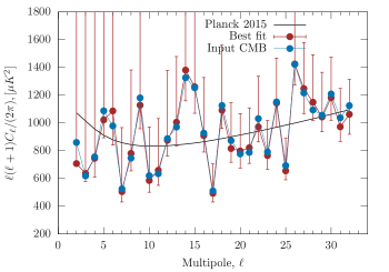
Figure 8.— Figure showing the best-fit estimate of theoretical CMB angular power spectrum (in brown) with $68.27\%$ confidence intervals for different multipoles along with the CMB angular power spectrum (in blue) estimated from the specific CMB realization used in the Monte Carlo simulations. The black line indicates the theoretical angular power spectrum from which the specific CMB realization under consideration is generated.

We show the best-fit estimate of underlying CMB theoretical angular power spectrum from Monte Carlo simulations in Fig. 8 in brown line. The asymmetric error-limits shown on this power spectrum indicate the $68.27\%$ confidence intervals. The angular power spectrum for the input CMB map used in the simulation is shown in blue. The best-fit estimate agrees nicely with the input angular power spectrum. The black line of this figure represents the underlying theoretical angular power spectrum that is used to generate the input CMB realization for the simulation.

We test the Gibbs sequences obtained from the simulations for convergence as in Section 5 using the Gelman-Rubin statistic, $R$. The maximum and minimum values of $R$ for the sampled CMB maps over all pixels are respectively, $1.00017$ and $0.999924$. The corresponding values for the sampled angular power spectra are respectively, $1.00027$ and $0.999935$. Such values of $R$ close to unity indicate convergence of the Gibbs sequences in Monte Carlo simulations.

7. Discussions and Conclusions

In this article, we have presented a new method to estimate the CMB posterior density over the large angular scales of the sky, given the Planck and WMAP observations by using a global ILC method (Sudevan & Saha, 2017) and Gibbs sampling (Gelman & Rubin, 1992) as the basic tools. Our main results are joint estimates of best-fit CMB signal and its theoretical angular power spectrum along with the appropriate confidence intervals which can be directly used for cosmological parameter estimation. Therefore, our work, for the first time effectively extends the ILC method for such purposes. We sample the CMB signal at each Gibbs iteration conditioning on a set of CMB theoretical angular power spectrum obtained in the previous Gibbs iteration. The CMB reconstruction step is independent on any explicit model of foreground components - which is a characteristic of the usual ILC method. However, considering the sampling of both CMB signal and its theoretical angular power spectrum, the new method extends the model independent nature of CMB reconstruction of ILC method to the entire posterior density estimation at low resolution. Thus our method serves as a complementary route to the CMB posterior estimation where detailed model of foregrounds are taken into account. We have implemented the CMB reconstruction method in the harmonic space which reduces computational time significantly unlike the pixel-space approach of Sudevan & Saha (2017).

There are some aspects of the method which one needs to address in future investigations. In the current work we have assumed that the detector noise can be completely ignored which is a valid assumption on the large angular scales for experiments like WMAP and Planck. A general framework will be to formalize the method in the presence of detector noise. In the presence of detector noise the blind foreground removal procedure will leave some foreground residuals on the cleaned maps. It would be interesting to see whether these residuals can be taken care of using a foreground model independent manner.

In the current method where detector noise is assumed to be negligible residual foregrounds will be present in the cleaned maps if effective number of foreground components $n_{f}$ present in the input frequency maps become larger than or equal to number of input frequency maps ($n$) available. For large angular scale analysis like the one of this paper, $n_{f}<n$ is a reasonable assumption outside the galactic plane. Along the plane, where the foreground spectral properties are expected show a larger variation than the outside plane, the effect of such residuals are mitigated by the smoothing of the input sky maps over the large angular scales. By performing detailed Monte Carlo simulations we see that the method leaves a small residual along the galactic plane. By comparing our cleaned map and angular power spectrum results with those obtained by other science groups we show that the level of such foreground residuals are small and of comparable magnitudes of those present in CMB maps obtained by other methods.

We thank an anonymous referee of an earlier publication by the authors (Sudevan & Saha, 2017) for suggestions of integrating the work with Gibbs sampling. Our work is based on observations obtained with Planck (http://www.esa.int/Planck), an ESA science mission with instruments and contributions directly funded by ESA Member States, NASA, and Canada. We use publicly available HEALPix Górski et al. (2005) package (http://healpix.sourceforge.net) for some of the analysis of this work. We acknowledge the use of Planck Legacy Archive (PLA) and the Legacy Archive for Microwave Background Data Analysis (LAMBDA). LAMBDA is a part of the High Energy Astrophysics Science Archive Center (HEASARC). HEASARC/LAMBDA is supported by the Astrophysics Science Division at the NASA Goddard Space Flight Center.

Appendix A A: Elements of Matrix ${\bf A}$ in Harmonic Space

Let us assume that, $S(p)$ denotes a random simulation of a pixellized CMB map ($p$ denotes pixel index) at some beam and pixel resolutions. Using the spherical harmonic decomposition $S(p)=\sum_{\ell,m}a_{\ell,m}Y_{\ell m}(p)$, the $(p,q)$ element, $C_{pq}$ of the pixel-pixel CMB covariance matrix, ${\bf C}$ can be written as

$$C_{pq}=\left<S(p)S(q)\right>=\sum_{\ell m\ell^{\prime}m^{\prime}}\left<a_{\ell m}a^{*}_{\ell^{\prime}m^{\prime}}\right>Y_{\ell m}(p)Y^{*}_{\ell^{\prime}m^{\prime}}(q)\,,$$ (A1)

where $\left<...\right>$ represents ensemble average and we assume that the beam and pixel smoothing effects are implicitly contained in spherical harmonic coefficients $a_{\ell m}$. Using statistical isotropy of CMB, namely, $\left<a_{\ell m}a^{*}_{\ell^{\prime}m^{\prime}}\right>=C^{\prime}_{\ell}\delta_{\ell\ell^{\prime}}\delta_{mm^{\prime}}$, where $C^{\prime}_{\ell}=C_{\ell}B^{2}_{\ell}P^{2}_{\ell}$, ($B_{\ell}$ and $P_{\ell}$ being respectively beam and pixel window functions) we obtain,

$$C_{pq}=\sum_{\ell m}C^{\prime}_{\ell}Y_{\ell m}(p)Y^{*}_{\ell m}(q)\,.$$ (A2)

In matrix notation we write Eqn. A2 as

$${\bf C}=\sum_{\ell m}C^{\prime}_{\ell}{\bf D}_{\ell m}\,,$$ (A3)

where elements of matrix ${\bf D}_{\ell m}$ are given by $D^{pq}_{\ell m}=Y_{\ell m}(p)Y^{*}_{\ell^{\prime}m^{\prime}}(q)$. We can write, ${\bf D}_{\ell m}={\bf Z}_{\ell m}{\bf Z}^{c}_{\ell m}$, where, ${\bf Z}_{\ell m}$ is an $N\times 1$ column vector with elements $Z_{\ell m}(p)=Y_{\ell m}(p)$, and the superscript ^c represents the Hermitian conjugate. It is worth emphasizing that, the right hand side of above equation represents a linear combination of ${\bf D}_{\ell m}$ matrices with the scalar amplitudes given by $C^{\prime}_{\ell}$. Clearly, therefore,

$${\bf C}^{\dagger}=\sum_{\ell m}{\bf D}^{\dagger}_{\ell m}C^{\prime\dagger}_{\ell}\,.$$ (A4)

Using the definition of Moore-Penrose generalized inverse, ${\bf x}^{\dagger}$ of a vector ${\bf x}$, ${\bf x}^{\dagger}={\bf x}^{c}/||{\bf x}||^{2}$ where $||...||^{2}$ represent squared norm of the vector, one obtains,

$${\bf D}^{\dagger}_{\ell m}=\frac{{\bf Z}_{\ell m}{\bf Z}^{c}_{\ell m}}{||{\bf Z}_{\ell m}||^{4}}\,.$$ (A5)

Using orthogonality of spherical harmonics over discrete HEALPix pixels

$$\left[\sum_{p=1}^{N}Y_{\ell m}(p)Y^{*}_{\ell m}(p)\right]\frac{4\pi}{N}=1\,,$$ (A6)

it is easy to find $||{\bf Z}_{\ell m}||^{4}=\left(N/(4\pi)\right)^{2}$. Using this result and Eqn. A5 in Eqn. A4 we obtain element wise,

$$C^{\dagger}_{pq}=\sum_{\ell m}\frac{1}{C^{\prime}_{\ell}}\frac{Y_{\ell m}(p)Y^{*}_{\ell m}(q)}{\left(\frac{N}{4\pi}\right)^{2}}\,,$$ (A7)

where we have used $C^{\prime\dagger}_{\ell}=1/C^{\prime}_{\ell}$. Expanding the input frequency maps ${\bf X}_{i}$ in spherical harmonic space, $X_{i}(p)=\sum_{\ell_{1}m_{1}}a^{i}_{\ell_{1},m_{1}}Y_{\ell_{1}m_{1}}(p)$, using Eqn. A7 and the orthogonality condition of spherical harmonics as mentioned in Eqn. A6, after some algebra, we obtain,

$$\hat{A}_{ij}={\bf X}^{T}_{i}{\bf C}^{\dagger}{\bf X}_{j}=\sum_{\ell}\left(2\ell+1\right)\frac{\hat{\sigma}^{ij}_{\ell}}{C^{\prime}_{\ell}}\,,$$ (A8)

where

$$\hat{\sigma}^{ij}_{\ell}=\sum_{m=-\ell}^{\ell}a^{i}_{\ell m}a^{j*}_{\ell m}/\left(2\ell+1\right)\,.$$ (A9)

Appendix B B: Conditional Density of CMB Theoretical Angular Power Spectrum

We note that, if $x_{1}$, $x_{2}$, …, $x_{\mu}$ are identically distributed and independent Gaussian random variable with zero mean and unit variance, the new variable $x=\sum_{k=1}^{\mu}x^{2}_{k}$ is distributed as a $\chi^{2}$ random variable with $\mu$ degrees of freedom, with the probability density given by,

$$P(x)=\frac{1}{2^{\nu}\Gamma(\nu)}x^{\nu-1}\exp\left[-\frac{x}{2}\right]\,,$$ (B1)

where $\nu=\mu/2$. With this definition, the variable $x\equiv\left(2\ell+1\right)\frac{\hat{C}_{\ell}}{C_{\ell}}$ is distributed as Eqn. B1, where $\hat{C}_{\ell}$ and $C_{\ell}$ respectively denote realization specific and theoretical CMB angular power spectrum. To find the density function of $\hat{C}_{\ell}$ we first note using Eqn. B1 that, the density function $Q(y)$ for the transformed variable $y=\beta x$ ($\beta$ = constant) follows, $Q(y)=P(x)dx/dy$, where in the right hand side $x$ must be replaced by $y$ using the inverse transformation $x=y/\beta$, so that one gets a function of $y$ as required. Using this concept and defining $y\equiv\hat{C}_{\ell}=C_{\ell}x/(2\ell+1)$, so that, $\beta=C_{\ell}/(2\ell+1)$, we find,

$$Q(\hat{C}_{\ell})=\left[2^{\left(2\ell+1\right)/2}\Gamma\left(\frac{2\ell+1}{2}\right)\right]^{-1}\left(\frac{2\ell+1}{C_{\ell}}\right)^{\left(2\ell+1\right)/2}{\hat{C}}^{\left(2\ell+1\right)/2-1}_{\ell}\exp\left[-\frac{\hat{C}_{\ell}\left(2\ell+1\right)}{2C_{\ell}}\right]$$ (B2)

Assuming $C_{\ell}$ as a random variable Eqn. B2 represents the conditional probability density $Q\left(\hat{C}_{\ell}|C_{\ell}\right)$. Using Bayes theorem and an uniform prior on $C_{\ell}$ upto some irrelevant constant, probability density of $C_{\ell}$ given some $\hat{C}_{\ell}$ can be obtained as,

$$R\left(C_{\ell}|\hat{C}_{\ell}\right)\propto\left(\frac{1}{C_{\ell}}\right)^{\left(2\ell+1\right)/2}\exp\left[-\frac{\hat{C}_{\ell}\left(2\ell+1\right)}{2C_{\ell}}\right]$$ (B3)

Now defining a new variable $z={\hat{C}_{\ell}\left(2\ell+1\right)}/{C_{\ell}}$ and noting that the exponent of $1/C_{\ell}$ in Eqn. B3 can be written as $(2\ell+1)/2=(2\ell-1)/2+1$ we can write Eqn. B3 as,

$$R\left(z|\hat{C}_{\ell}\right)\propto z^{-(2\ell-1)/2-1}\exp\left[-\frac{z}{2}\right]\,,$$ (B4)

where we have omitted some irrelevant constants. Comparing Eqn. B4 with Eqn. B1 we readily identify Eqn. B4 as a $\chi^{2}$ distribution of $2\ell-1$ degrees of freedom in variable $z$.

References

- Basak & Delabrouille (2012) Basak, S., & Delabrouille, J. 2012, MNRAS, 419, 1163
- Basak & Delabrouille (2013) —. 2013, MNRAS, 435, 18
- Bennett et al. (1992) Bennett, C. L., Smoot, G. F., Hinshaw, G., et al. 1992, ApJ, 396, L7
- Bennett et al. (2003) Bennett, C. L., Hill, R. S., Hinshaw, G., et al. 2003, ApJS, 148, 97
- Bennett et al. (2013) Bennett, C. L., Larson, D., Weiland, J. L., et al. 2013, ApJS, 208, 20
- Bouchet & Gispert (1999) Bouchet, F. R., & Gispert, R. 1999, New A, 4, 443
- Bouchet et al. (1999) Bouchet, F. R., Prunet, S., & Sethi, S. K. 1999, MNRAS, 302, 663
- Brooks & Gelman (1998) Brooks, S. P., & Gelman, A. 1998, Journal of Computational and Graphical Statistics, 7, 434
- Bunn et al. (1994) Bunn, E. F., Fisher, K. B., Hoffman, Y., et al. 1994, ApJ, 432, L75
- Eriksen et al. (2004a) Eriksen, H. K., Banday, A. J., Górski, K. M., & Lilje, P. B. 2004a, ApJ, 612, 633
- Eriksen et al. (2008a) Eriksen, H. K., Dickinson, C., Jewell, J. B., et al. 2008a, ApJ, 672, L87
- Eriksen et al. (2008b) Eriksen, H. K., Jewell, J. B., Dickinson, C., et al. 2008b, ApJ, 676, 10
- Eriksen et al. (2004b) Eriksen, H. K., O’Dwyer, I. J., Jewell, J. B., et al. 2004b, ApJS, 155, 227
- Eriksen et al. (2006) Eriksen, H. K., Dickinson, C., Lawrence, C. R., et al. 2006, ApJ, 641, 665
- Eriksen et al. (2007) Eriksen, H. K., Huey, G., Saha, R., et al. 2007, ApJ, 656, 641
- Gelman & Rubin (1992) Gelman, A., & Rubin, D. 1992, Statistical Science, 1, 457
- Geman & Geman (1984) Geman, S., & Geman, D. 1984, IEEE Trans. Pattern Anal. Mach. Intell., 6, 721
- Gold et al. (2011) Gold, B., Odegard, N., Weiland, J. L., et al. 2011, ApJS, 192, 15
- Górski et al. (2005) Górski, K. M., Hivon, E., Banday, A. J., et al. 2005, ApJ, 622, 759
- Hinshaw et al. (2013) Hinshaw, G., Larson, D., Komatsu, E., et al. 2013, ApJS, 208, 19
- Moore (1920) Moore, E. H. 1920, Bull. Am. Math. Soc., 26, 394, unpublished address. Available at http://www.ams.org/journals/bull/1920-26-09/S0002-9904-1920-03322-7/S0002-9904-1920-03322-7.pdf.
- Penrose (1955) Penrose, R. 1955, Mathematical Proceedings of the Cambridge Philosophical Society, 51, 406
- Penzias & Wilson (1965) Penzias, A. A., & Wilson, R. W. 1965, ApJ, 142, 419
- Planck Collaboration et al. (2016a) Planck Collaboration, Adam, R., Ade, P. A. R., et al. 2016a, A&A, 594, A9
- Planck Collaboration et al. (2016b) —. 2016b, A&A, 594, A9
- Planck Collaboration et al. (2016c) —. 2016c, A&A, 594, A10
- Planck Collaboration et al. (2016d) Planck Collaboration, Ade, P. A. R., Aghanim, N., et al. 2016d, A&A, 594, A13
- Planck Collaboration et al. (2018a) Planck Collaboration, Akrami, Y., Arroja, F., et al. 2018a, ArXiv e-prints, arXiv:1807.06205
- Planck Collaboration et al. (2018b) Planck Collaboration, Akrami, Y., Ashdown, M., et al. 2018b, ArXiv e-prints, arXiv:1807.06208
- Purkayastha & Saha (2017) Purkayastha, U., & Saha, R. 2017, ArXiv e-prints, arXiv:1707.02008
- Saha (2011) Saha, R. 2011, ApJ, 739, L56
- Saha & Aluri (2016) Saha, R., & Aluri, P. K. 2016, ApJ, 829, 113
- Saha et al. (2006) Saha, R., Jain, P., & Souradeep, T. 2006, ApJ, 645, L89
- Saha et al. (2008) Saha, R., Prunet, S., Jain, P., & Souradeep, T. 2008, Phys. Rev. D, 78, 023003
- Smoot et al. (1991) Smoot, G. F., Bennett, C. L., Kogut, A., et al. 1991, ApJ, 371, L1
- Sudevan et al. (2017) Sudevan, V., Aluri, P. K., Yadav, S. K., Saha, R., & Souradeep, T. 2017, ApJ, 842, 62
- Sudevan & Saha (2017) Sudevan, V., & Saha, R. 2017, ArXiv e-prints, arXiv:1712.09804
- Tegmark et al. (2003) Tegmark, M., de Oliveira-Costa, A., & Hamilton, A. J. 2003, Phys. Rev. D, 68, 123523
- Tegmark & Efstathiou (1996) Tegmark, M., & Efstathiou, G. 1996, Mon. Not. R. Astron. Soc., 281, 1297