Pose consensus based on dual quaternion algebra with application to decentralized formation control of mobile manipulators

Abstract

This paper presents a solution based on dual quaternion algebra to the general problem of pose (i.e., position and orientation) consensus for systems composed of multiple rigid-bodies. The dual quaternion algebra is used to model the agents’ poses and also in the distributed control laws, making the proposed technique easily applicable to time-varying formation control of general robotic systems. The proposed pose consensus protocol has guaranteed convergence when the interaction among the agents is represented by directed graphs with directed spanning trees, which is a more general result when compared to the literature on formation control. In order to illustrate the proposed pose consensus protocol and its extension to the problem of formation control, we present a numerical simulation with a large number of free-flying agents and also an application of cooperative manipulation by using real mobile manipulators.

1 Introduction

Recent technological advances have enabled the use of distributed multi-agent systems in the solution of different real-world problems. In fact, replacing a single complex agent by multiple yet simpler ones yields many benefits such as flexibility, fault tolerance, cost reduction, etc., which justifies the development of decentralized controllers for this class of systems. There exist many results regarding the use of decentralized controllers in autonomous systems such as formation control of autonomous vehicles [1, 2], networked robotics [3, 4], etc. Many other results are summarized in [5].

Some decentralized strategies are based on the solution of a consensus problem, whose main objective is to enable agents in a multi-agent system to reach an agreement about some variable of interest by means of local distributed control laws, called consensus protocols. These protocols rely on the assumption that each agent has access to the information provided by only a subset of agents, called neighbors. This subset is defined according to an interaction network that is usually modeled by a graph. The problem of achieving consensus based only on neighbors interactions was initially proposed in [6] and algebraically formulated in the works of [7, 8].

On the application side, an interesting use of consensus-based algorithms is in the solution of decentralized formation control problems in multi-agent systems [2] and robotics [9]. In fact, several tasks may benefit from solutions of formation control, such as load transportation with cooperative robots to move flexible payloads [10]. Different formation control scenarios have been investigated such as the ones incorporating, but not limited to, time-varying formations [11, 12, 13, 14], formations with multiple leaders [15, 16, 17], switching network topologies [18, 19, 20], time-delays [21, 22], etc. Stochastic switching topologies with time-varying delays have also been considered in [23].

Devising new solutions for different aspects of consensus and formation control problems is still an active research topic. Some recent studies have considered multi-agent systems composed of rigid-body agents, usually with the objective of achieving a common orientation or, more generally, a common pose (position and orientation). Hatanaka et al. [4], for example, use homogeneous representations to describe the complete pose and make use of passivity theory to show consensus in the case of strongly connected networks. Mayhew et al. [24] show consensus in the orientation for undirected networks by applying a hybrid controller and a representation based on quaternions. Sarlette et al. [25] show relaxed conditions for directed and varying networks. Aldana et al. [26] decoupled agents’ positions and orientations expressing poses as two independent entities, position vectors and orientation quaternions, and addressed leader-follower and leaderless pose-consensus problems in undirected networks. The same authors [27] extend the previous results to consensus problems in the operational space of robotic manipulators without velocity measurements. Wang et al. [28] consider dual quaternions to represent the pose and propose a control law based on the logarithm of dual quaternions to show consensus in networks with rooted-tree topologies. Wang and Yu [29] also consider dual quaternions for leader-followers in undirected topologies. The logarithm of a quaternion was defined by [30], which served as base for the logarithmic controller proposed by [28].

In networks composed of multiple robotic manipulators, described as rigid-body agents, the agents can be modeled with dual quaternions [31] and consensus theory can be used to analyze or design distributed control laws. Some advantages of using quaternions and dual quaternions in formation control are shown by Mas and Kitts [32] in the framework of Cluster Space Control, by defining each relative position of the agents by means of relative transformations given by dual quaternions. An application on formation of unmanned aerial vehicles is shown in [33].

A growing interest in dual quaternions for rigid-body pose consensus and formation control arises from the many benefits of using dual quaternion algebra. As pointed by [34], it is straightforward to use dual quaternions in the representation of rigid motions, twists, wrenches, and several geometric primitives—e.g., Plücker lines and planes. In addition, dual quaternions are more compact than homogeneous transformation matrices (HTM)—the former has only eight parameters whereas the latter has sixteen—and dual quaternion multiplications have lower computational cost than HTM multiplications [31]. Furthermore, unit dual quaternions do not have representational singularities (although this feature is also present in HTM) and, given a unit dual quaternion, it is easy to extract relevant geometric parameters as, for example, translation, axis of rotation, and angle of rotation. Moreover, dual quaternions are easily mapped into a vector structure, which can be particularly convenient when controlling a robot as they can be used directly in the control law. Finally, complex systems (e.g., mobile manipulators and humanoids) can be easily modeled with dual quaternions using a whole-body approach [31, 35]. Thanks to the aforementioned advantages, dual quaternions are used throughout the paper as the main mathematical tool for representing poses and rigid motions.

1.1 Statement of Contributions and Paper Organization

The contributions of this paper are the following:

1. First, we derive a logarithmic differentiable mapping of dual quaternions, extending the result in [30]. This allows a straightforward theoretical connection between the myriad of results of rigid-body modeling based on dual quaternion algebra and the results of linear consensus theory applied to Euclidean spaces. The advantage of such connection is that previous results in linear consensus theory for time-delays and switching topologies in Euclidean spaces, such as the ones presented in [23], may be easily applied to the problem of formation control of rigid bodies, which is non-linear and whose underlying topological space is a non-Euclidean manifold;

2. Next, by defining the agent’s output as the logarithmic mapping of the unit dual quaternion corresponding to the agent’s pose, we propose a pose-consensus protocol with guaranteed convergence for scenarios where the interaction graphs are given by directed graphs with directed spanning trees, which is a more general case when compared to previous results, for instance, the ones in [28, 26, 27, 4]. It is important to note that guaranteeing consensus in the pose is not a trivial task as unit dual quaternions lie in a non-Euclidean topological space (more specifically, unit dual quaternions belong to the Lie group $\text{Spin(3)}\ltimes\mathbb{R}^{3}$, whose underlying manifold is $\mathbb{S}^{3}\times\mathbb{R}^{3}$ [36]);

3. Different from other works such as [26, 27], we propose a consensus-based strategy for decentralized formation control of rigid-bodies in which both position and orientation are treated in a unified manner, which allows to consider any arbitrary communication network containing a directed spanning tree. An extension to consider time-varying formations is also devised. This result is more general than the previous ones found in the literature that also focus on the formation control of systems composed of rigid bodies [28, 32, 33, 29] as our approach: (i) is decentralized in the sense that only neighbor information is needed by each agent, in contrast to the necessity of obtaining global information such as the state variables of a shape or of a leader as in [32, 33]; and (ii) is also able to deal with general directed graph topologies, in contrast to the requirement of imposing some specific graph topologies such as undirected graphs [29] and rooted trees [28];

4. On the application side, whole-body control and consensus protocols are used to propose a strategy that allows decentralized formation control of the end-effectors of mobile manipulators whose kinematic models are given directly in the algebra of dual quaternions;

5. Finally, the proposed strategy is verified by means of numerical simulations and also in a real-world cooperative manipulation task.

The paper is organized as follows. Section 2 presents a brief mathematical background whereas Section 3 presents the differential logarithmic mapping of unit dual quaternions, which is of central importance in the development of the pose-consensus protocols proposed in Section 4. In Section 5 we solve the problem of formation control of multiple rigid-bodies by using dual quaternion algebra. Section 6 shows a numerical simulation with a large number of agents to illustrate the results and scalability of the proposed method, and also shows the formation control applied to real robots in a cooperative manipulation task. Finally, Section 7 concludes the paper and provides indications of future works.

2 Mathematical Preliminaries

This section briefly presents the main mathematical tools and notations used throughout the paper. For more information on the algebraic formulation of the consensus problem and dual quaternion algebra, please refer to [8] and [37], respectively.

2.1 Algebraic Graph Theory

The information flow of the multi-agent system is represented by a simple directed graph. Let a simple weighted directed graph be defined by the ordered triplet $\mathcal{G}\left(\mathcal{V},\mathcal{E},\bm{A}\right)$, where: $\mathcal{V}$ is a set of $n\in\mathbb{N}$ vertices (nodes) arbitrarily labeled as $v_{1},v_{2},\ldots,v_{n}$; the set $\mathcal{E}$ contains the directed edges $e_{ij}=(v_{i},v_{j})$ that connect the vertices, where the first element $v_{i}\in\mathcal{V}$ is said to be the parent node (tail) and the latter, $v_{j}\in\mathcal{V}$, to be the child node (head); and $\bm{A}=[a_{ij}]$ is the adjacency matrix of order $n\times n$ related to the edges that assigns a real non-negative weight value for each $e_{ji}$:

$$a_{ij}\begin{cases}=0,&\text{if }i=j\text{ or }\nexists e_{ji},\\ >0,&\text{iff }\exists e_{ji}.\end{cases}$$ (1)

The degree matrix $\bm{\Delta}=[\Delta_{ij}]$, which is related to $\bm{A}$, is a diagonal matrix with elements $\Delta_{ii}=\sum_{j=1}^{n}a_{ij}$. The Laplacian matrix associated to the graph $\mathcal{G}$ is given by $\bm{L}=\bm{\Delta}-\bm{A}$, and the following property holds:

$$\bm{L}\bm{1}_{n} =\bm{0}_{n},$$ (2)

where $\bm{1}_{n}$ and $\bm{0}_{n}$ are $n$-dimensional column-vectors of ones and zeros, respectively.

A directed tree is a directed graph with only one node without parent nodes (or without directed edges pointing towards it) called root, and all other nodes having exactly one parent. Also, there is a path, i.e. a sequence of edges, connecting the root to any other node in the tree. A directed spanning tree is a directed tree that can be formed from the removal of some of the edges of a directed graph, such that all nodes are included and there is a unique directed path from the root node to any other node in the graph.

2.2 Quaternions and dual quaternions

Quaternions can be regarded as an extension of complex numbers, and the quaternion set is defined as

$$\mathbb{H} \triangleq\left\{h_{1}+\hat{\imath}h_{2}+\hat{\jmath}h_{3}+\hat{k}h_{4}\,:\,h_{1},h_{2},h_{3},h_{4}\in\mathbb{R}\right\},$$ (3)

in which the imaginary units $\hat{\imath}$, $\hat{\jmath}$, and $\hat{k}$ have the following properties:

$$\hat{\imath}^{2} =\hat{\jmath}^{2}=\hat{k}^{2}=\hat{\imath}\hat{\jmath}\hat{k}=-1.$$ (4)

Addition and multiplication are defined for quaternions analogously to complex numbers (i.e., in the usual way), and one just needs to respect the properties in (4) for the imaginary units. Given $\bm{h}\in\mathbb{H}$, such that $\bm{h}=h_{1}+\hat{\imath}h_{2}+\hat{\jmath}h_{3}+\hat{k}h_{4}$, we define $\operatorname{\mathrm{Re}}\left(\bm{h}\right)\triangleq h_{1}$ and $\operatorname{\mathrm{Im}}\left(\bm{h}\right)\triangleq\hat{\imath}h_{2}+\hat{\jmath}h_{3}+\hat{k}h_{4}$. The conjugate of $\bm{h}$ is defined as $\bm{h}^{*}\triangleq\operatorname{\mathrm{Re}}\left(\bm{h}\right)-\operatorname{\mathrm{Im}}\left(\bm{h}\right)$ and its norm is given by $\left\|\bm{h}\right\|\triangleq\sqrt{\bm{h}^{*}\bm{h}}=\sqrt{\bm{h}\bm{h}^{*}}.$

The set

$$\mathbb{H}_{p} \triangleq\left\{\bm{h}\in\mathbb{H}\,:\,\operatorname{\mathrm{Re}}\left(\bm{h}\right)=0\right\}$$ (5)

is usually called the set of pure quaternions and has a bijective relation with $\mathbb{R}^{3}$. Hence, the quaternion $\left(x\hat{\imath}+y\hat{\jmath}+z\hat{k}\right)\in\mathbb{H}_{p}$ represents the point $\left(x,y,z\right)\in\mathbb{R}^{3}$ [38]. The set of quaternions with unit norm is defined as

$$\mathbb{S}^{3} \triangleq\left\{\bm{h}\in\mathbb{H}\,:\,\left\|\bm{h}\right\|=1\right\},$$ (6)

and elements of $\mathbb{S}^{3}$ equipped with the multiplication operation form the group of rotations $\text{Spin}(3)$, which double covers $\mathrm{SO}\left(3\right)$. A unit quaternion $\bm{r}\in\mathbb{S}^{3}$ represents a rotation from an inertial frame $\mathcal{F}$ to frame $\mathcal{F}_{i}$ and can always be written as

$$\bm{r}_{i} =\cos\left(\frac{\phi_{i}}{2}\right)+\sin\left(\frac{\phi_{i}}{2}\right)\bm{n}_{i},$$ (7)

where $\phi_{i}\in\mathbb{R}$ is a rotation angle around the rotation axis $\bm{n}_{i}\in\mathbb{S}^{3}\cap\mathbb{H}_{p}$ [37]. Notice that $\bm{n}_{i}$ is pure (hence it is equivalent to a vector in $\mathbb{R}^{3}$) and has unit norm.

The set of dual quaternions extends the set of quaternions and is defined as

$$\mathcal{H} \triangleq\left\{\bm{h}+\epsilon\bm{h}^{\prime}\,:\,\bm{h},\bm{h}^{\prime}\in\mathbb{H},\,\varepsilon^{2}=0,\,\varepsilon\neq 0\right\},$$ (8)

where $\varepsilon$ is usually called dual (or Clifford) unit [38]. Similarly to quaternions, addition and multiplication are defined in the usual way, and one just needs to respect the properties of the imaginary and dual units.

Given $\underline{\bm{h}}\in\mathcal{H}$ such that $\underline{\bm{h}}=h_{1}+\hat{\imath}h_{2}+\hat{\jmath}h_{3}+\hat{k}h_{4}+\varepsilon\left(h_{1}^{\prime}+\hat{\imath}h_{2}^{\prime}+\hat{\jmath}h_{3}^{\prime}+\hat{k}h_{4}^{\prime}\right)$, we define the operators

$$\begin{split}\operatorname{\mathrm{Re}}\left(\underline{\bm{h}}\right)&\triangleq h_{1}+\varepsilon h_{1}^{\prime},\\ \operatorname{\mathrm{Im}}\left(\underline{\bm{h}}\right)&\triangleq\hat{\imath}h_{2}+\hat{\jmath}h_{3}+\hat{k}h_{4}+\varepsilon\left(\hat{\imath}h_{2}^{\prime}+\hat{\jmath}h_{3}^{\prime}+\hat{k}h_{4}^{\prime}\right).\end{split}$$

Analogously to quaternions, the conjugate of $\underline{\bm{h}}\in\mathcal{H}$ is defined as $\underline{\bm{h}}^{*}\triangleq\operatorname{\mathrm{Re}}\left(\underline{\bm{h}}\right)-\operatorname{\mathrm{Im}}\left(\underline{\bm{h}}\right)$, and its norm is given by $\left\|\underline{\bm{h}}\right\|\triangleq\sqrt{\underline{\bm{h}}\underline{\bm{h}}^{*}}=\sqrt{\underline{\bm{h}}^{*}\underline{\bm{h}}}$.

The set

$$\mathcal{H}_{p}\triangleq\left\{\underline{\bm{h}}\in\mathcal{H}\,:\,\operatorname{\mathrm{Re}}\left(\underline{\bm{h}}\right)=0\right\}$$

is called set of pure dual quaternions and is isomorphic to $\mathbb{R}^{6}$. Some physical objects—for instance, twists (i.e., linear and angular velocities) and wrenches (i.e., forces and moments)—can be represented as elements of $\mathcal{H}_{p}$ [37].

Elements of the set

$$\underline{\bm{\mathcal{S}}} \triangleq\left\{\underline{\bm{h}}\in\mathcal{H}\,:\,\left\|\underline{\bm{h}}\right\|=1\right\}$$

are called unit dual quaternions. The set $\underline{\bm{\mathcal{S}}}$ equipped with the multiplication operation form the group $\text{Spin}(3){\ltimes}\mathbb{R}^{3}$, which double covers $\mathrm{SE}\left(3\right)$. A unit dual quaternion $\underline{\bm{x}}\in\underline{\bm{\mathcal{S}}}$ represents a rigid motion from an inertial frame $\mathcal{F}$ to frame $\mathcal{F}_{i}$ and is represented by

$$\underline{\bm{x}}_{i} =\bm{r}_{i}+\varepsilon\frac{1}{2}\bm{p}_{i}\bm{r}_{i},$$ (9)

where $\bm{r}_{i}\in\mathbb{S}^{3}$ and $\bm{p}_{i}\in\mathbb{H}_{p}$ represent the rotation and translation, respectively [38].

Since $\text{Spin}(3)$ and $\text{Spin}(3)\ltimes\mathbb{R}^{3}$ are non-commutative groups—analogously to $\mathrm{SO}\left(3\right)$ and $\mathrm{SE}\left(3\right)$—, quaternions and dual quaternions are non-commutative under multiplication. However, we can use the Hamilton operators, which are matrices defined in [39, 37] for both quaternions and dual quaternions, that can be used to commute these terms in algebraic expressions such that, for $\bm{h}_{1},\bm{h}_{2}\in\mathbb{H}$ and $\underline{\bm{h}}_{1},\underline{\bm{h}}_{2}\in\mathcal{H}$,

$$\operatorname{vec}_{4}(\bm{h}_{1}\bm{h}_{2}) =\overset{+}{\bm{H}}_{4}(\bm{h}_{1})\operatorname{vec}_{4}\bm{h}_{2}=\overset{-}{\bm{H}}_{4}(\bm{h}_{2})\operatorname{vec}_{4}\bm{h}_{1},$$ (10)

$$\operatorname{vec}_{8}(\underline{\bm{h}}_{1}\underline{\bm{h}}_{2}) =\overset{+}{\bm{H}}_{8}(\underline{\bm{h}}_{1})\operatorname{vec}_{8}\underline{\bm{h}}_{2}=\overset{-}{\bm{H}}_{8}(\underline{\bm{h}}_{2})\operatorname{vec}_{8}\underline{\bm{h}}_{1},$$ (11)

where $\operatorname{vec}_{4}\bm{h}=\begin{bmatrix}h_{1}&\cdots&h_{4}\end{bmatrix}^{T}$ and $\operatorname{vec}_{8}\underline{\bm{h}}=\begin{bmatrix}h_{1}&\cdots&h_{8}\end{bmatrix}^{T}$ are mappings of quaternions into $\mathbb{R}^{4}$ and dual quaternions into $\mathbb{R}^{8}$, respectively; i.e, $\operatorname{vec}_{4}:\mathbb{H}\rightarrow\mathbb{R}^{4}$ and $\operatorname{vec}_{8}:\mathcal{H}\rightarrow\mathbb{R}^{8}$.The Hamilton operators are given explicitly by

$$\overset{+}{\bm{H}}_{4}\left(\bm{h}\right) =\begin{bmatrix}h_{1}&-h_{2}&-h_{3}&-h_{4}\\ h_{2}&h_{1}&-h_{4}&h_{3}\\ h_{3}&h_{4}&h_{1}&-h_{2}\\ h_{4}&-h_{3}&h_{2}&h_{1}\end{bmatrix}, \overset{-}{\bm{H}}_{4}\left(\bm{h}\right) =\begin{bmatrix}h_{1}&-h_{2}&-h_{3}&-h_{4}\\ h_{2}&h_{1}&h_{4}&-h_{3}\\ h_{3}&-h_{4}&h_{1}&h_{2}\\ h_{4}&h_{3}&-h_{2}&h_{1}\end{bmatrix},$$ (12)

$$\overset{+}{\bm{H}}_{8}\left(\underline{\bm{h}}\right) =\begin{bmatrix}\overset{+}{\bm{H}}_{4}\left(\bm{h}\right)&\bm{0}_{4\times 4}\\ \overset{+}{\bm{H}}_{4}\left(\bm{h}^{\prime}\right)&\overset{+}{\bm{H}}_{4}\left(\bm{h}\right)\end{bmatrix}, \overset{-}{\bm{H}}_{8}\left(\underline{\bm{h}}\right) =\begin{bmatrix}\overset{-}{\bm{H}}_{4}\left(\bm{h}\right)&\bm{0}_{4\times 4}\\ \overset{-}{\bm{H}}_{4}\left(\bm{h}^{\prime}\right)&\overset{-}{\bm{H}}_{4}\left(\bm{h}\right)\end{bmatrix}.$$ (13)

We also define the mappings $\operatorname{vec}_{3}\,:\,\mathbb{H}_{p}\rightarrow\mathbb{R}^{3}$ and $\operatorname{vec}_{6}\,:\,\mathcal{H}_{p}\rightarrow\mathbb{R}^{6}$. Thus, given a pure quaternion $\bm{h}\in\mathbb{H}_{p}$ such that $\bm{h}=\operatorname{\mathrm{Im}}\left(\bm{h}\right)=h_{1}\hat{\imath}+h_{2}\hat{\jmath}+h_{3}\hat{k}$, then $\operatorname{vec}_{3}\bm{h}=\begin{bmatrix}h_{1}&h_{2}&h_{3}\end{bmatrix}^{T}$. Analogously, given a pure dual quaternion $\underline{\bm{h}}\in\mathcal{H}_{p}$ such that $\underline{\bm{h}}=\operatorname{\mathrm{Im}}\left(\underline{\bm{h}}\right)=h_{1}\hat{\imath}+h_{2}\hat{\jmath}+h_{3}\hat{k}+\varepsilon\left(h_{4}\hat{\imath}+h_{5}\hat{\jmath}+h_{6}\hat{k}\right)$, then $\operatorname{vec}_{6}\underline{\bm{h}}=\begin{bmatrix}h_{1}&\cdots&h_{6}\end{bmatrix}^{T}$.

The logarithm of a unit quaternion given as in (7) yields [30]

$$\log\bm{r}_{i} \triangleq\frac{\phi_{i}}{2}\bm{n}_{i}.$$ (14)

Similarly, the logarithm of a unit dual quaternion given as in (9) is defined as [40]:

$$\log\underline{\bm{x}}_{i} \triangleq\frac{1}{2}(\phi_{i}\bm{n}_{i}+\varepsilon\bm{p}_{i}),$$ (15)

where $\log\underline{\bm{x}}_{i}\in\mathcal{H}_{p}$.

Let $\underline{\bm{g}}\in\mathcal{H}_{p}$, such that $\underline{\bm{g}}=\bm{g}+\varepsilon\bm{g}^{\prime}$, the inverse mapping $\exp:\mathcal{H}_{p}\to\text{Spin}(3){\ltimes}\mathbb{R}^{3}$ is given by [31]

$$\exp\underline{\bm{g}} =\exp\bm{g}+\varepsilon\bm{g}^{\prime}\exp\bm{g},$$ (16)

$$\exp\bm{g} =\begin{cases}\cos\left\|\bm{g}\right\|+\frac{\sin\left\|\bm{g}\right\|}{\left\|\bm{g}\right\|}\bm{g}&\text{if }\bm{g}\neq 0,\\ 1&\text{otherwise.}\end{cases}$$ (17)

Therefore, $\underline{\bm{x}}=\exp(\log\underline{\bm{x}})$ and (16) is an injective mapping for $\phi_{i}\in[0,2\pi)$.

The twist $\underline{\bm{\xi}}_{i}\in\mathcal{H}_{p}$ of frame $\mathcal{F}_{i}$ expressed with respect to the inertial frame $\mathcal{F}$ is defined as

$$\underline{\bm{\xi}}_{i} \triangleq\bm{\omega}_{i}+\varepsilon(\dot{\bm{p}}_{i}+\bm{p}_{i}\times\bm{\omega}_{i}),$$ (18)

where $\bm{\omega}_{i}\in\mathbb{H}_{p}$ is the angular velocity and $\dot{\bm{p}}_{i}\in\mathbb{H}_{p}$ is the linear velocity. The cross-product for pure quaternions is given by

$$\bm{p}_{i}\times\bm{\omega}_{i}=\frac{\bm{p}_{i}\bm{\omega}_{i}-\bm{\omega}_{i}\bm{p}_{i}}{2},$$ (19)

which is equivalent to the vector cross-product in $\mathbb{R}^{3}$ thanks to the isomorphism between $\mathbb{H}_{p}$ and $\mathbb{R}^{3}$ under addition operations.

The derivative of $\underline{\bm{x}}_{i}$ can be expressed by [37]

$$\dot{\underline{\bm{x}}}_{i} =\frac{1}{2}\underline{\bm{\xi}}_{i}\underline{\bm{x}}_{i}.$$ (20)

3 The differential logarithmic mapping

In order to design the consensus protocols and the corresponding consensus-based formation controllers, we use the differential logarithmic mapping of dual quaternions. This differential mapping allows us to circumvent the difficulties related to the topology of the non-Euclidean manifold $\underline{\bm{\mathcal{S}}}$. Indeed, as shown in [36] the set $\underline{\bm{\mathcal{S}}}$ of unit dual quaternions can be regarded as the product manifold $\mathbb{S}^{3}\times\mathbb{R}^{3}$. Therefore, the consensus protocols usually found in the literature cannot be directly applied to elements of $\underline{\bm{\mathcal{S}}}$ because those protocols assume an $n$-dimensional Euclidean space.

We extend the results of Kim et al. [30], which were proposed only for quaternions, to derive the differential logarithm mapping for dual quaternions.

Lemma 1 ([30]).

Consider $\bm{r}\in\mathbb{S}^{3}$, with $\bm{r}=\cos\left(\phi/2\right)+\bm{n}\sin\left(\phi/2\right)$, where $\bm{n}\in\mathbb{S}^{3}\cap\mathbb{H}_{p}$ and $\phi\in\left[0,2\pi\right)$, and $\bm{y}=\left(y_{x}\hat{\imath}+y_{y}\hat{\jmath}+y_{z}\hat{k}\right)\in\mathbb{H}_{p}$ such that $\bm{y}=\log\bm{r}$. Thus

$$\frac{\partial\operatorname{vec}_{4}\bm{r}}{\partial\operatorname{vec}_{3}\bm{y}}=\begin{bmatrix}-ay_{x}&-ay_{y}&-ay_{z}\\ by_{x}^{2}+a&by_{x}y_{y}&by_{x}y_{z}\\ by_{x}y_{y}&by_{y}^{2}+a&by_{y}y_{z}\\ by_{x}y_{z}&by_{y}y_{z}&by_{z}^{2}+a\end{bmatrix},$$ (21)

where

$$a =\frac{\sin\left\|\bm{y}\right\|}{\left\|\bm{y}\right\|}, b =\frac{\cos\left\|\bm{y}\right\|}{\left\|\bm{y}\right\|^{2}}-\frac{\sin\left\|\bm{y}\right\|}{\left\|\bm{y}\right\|^{3}}$$

for $\bm{y}\neq 0$;

$$\frac{\partial\operatorname{vec}_{4}\bm{r}}{\partial\operatorname{vec}_{3}\bm{y}}=\begin{bmatrix}\bm{0}_{1\times 3}\\ \bm{I}_{3}\end{bmatrix},$$

if $\bm{y}=0$.

Proof.

See [30]. ∎

The entries of $\partial\operatorname{vec}_{4}\bm{r}/\partial\operatorname{vec}_{3}\bm{y}$, given in Theorem 1, depend on the coefficients of $\bm{y}$, which is the logarithm of $\bm{r}\in\mathbb{S}^{3}$. However, it is convenient to rewrite that matrix as a function of only the coefficients of $\bm{r}$ in order to exploit some useful properties later on.

Theorem 2 (Alternative form of Lemma 1).

Consider $\bm{r}=\left(r_{1}+r_{2}\hat{\imath}+r_{3}\hat{\jmath}+r_{4}\hat{k}\right)\in\mathbb{S}^{3}$, with $\bm{r}=\cos\left(\phi/2\right)+\bm{n}\sin\left(\phi/2\right)$, where $\bm{n}=\left(n_{x}\hat{\imath}+n_{y}\hat{\jmath}+n_{z}\hat{k}\right)\in\mathbb{S}^{3}\cap\mathbb{H}_{p}$ and $\phi\in\left[0,2\pi\right)$, and $\bm{y}=\left(y_{x}\hat{\imath}+y_{y}\hat{\jmath}+y_{z}\hat{k}\right)\in\mathbb{H}_{p}$ such that $\bm{y}\triangleq\log\bm{r}=\bm{n}\left(\phi/2\right)$. Thus,

$$\frac{\partial\operatorname{vec}_{4}\bm{r}}{\partial\operatorname{vec}_{3}\bm{y}}=\begin{bmatrix}-r_{2}&-r_{3}&-r_{4}\\ \Gamma n_{x}^{2}+\Theta&\Gamma n_{x}n_{y}&\Gamma n_{x}n_{z}\\ \Gamma n_{y}n_{x}&\Gamma n_{y}^{2}+\Theta&\Gamma n_{y}n_{z}\\ \Gamma n_{z}n_{x}&\Gamma n_{z}n_{y}&\Gamma n_{z}^{2}+\Theta\end{bmatrix},$$ (22)

where $\Gamma=r_{1}-\Theta$ and

$$\Theta=\begin{cases}1&\text{if }\phi=0,\\ \frac{\sin\left(\phi/2\right)}{\phi/2}&\text{otherwise.}\end{cases}$$

Proof.

First, let us denote the matrix (21) in Theorem 1 by $\bm{M}=\left[m_{ij}\right]$ and the matrix (22) by $\bm{Q}=\left[q_{ij}\right]$. For the case when $\phi=0$, $r_{1}=1$, we have $\Gamma=0$ and then, clearly, $\bm{M}=\bm{Q}=\begin{bmatrix}\bm{0}_{3\times 1}&\bm{I}_{3}\end{bmatrix}^{T}.$

In order to show that $\bm{M}=\bm{Q}$ when $\phi\neq 0$, we start by verifying the terms of the first row. Using Fact 16 (see A) we obtain

$$m_{11}=-\frac{\sin\left\|\bm{y}\right\|}{\left\|\bm{y}\right\|}\frac{\phi}{2}n_{x}=-\sin\left(\frac{\phi}{2}\right)n_{x}=-r_{2}=q_{11}.$$

Analogously, $m_{12}=-\sin\left(\phi/2\right)n_{y}=-r_{3}=q_{12}$ and $m_{13}=-\sin\left(\phi/2\right)n_{z}=-r_{4}=q_{13}$.

Thanks to the symmetry of the the last three rows of $\bm{M}$ and $\bm{Q}$ only a few terms must be verified, namely $q_{21}$, $q_{22}$, $q_{23}$, $q_{32}$, $q_{33}$, and $q_{43}$. Starting from $m_{21}$ and using Fact 16, we obtain

$$m_{21} =by_{x}^{2}+a$$

$$=\left(\frac{\cos\left\|\bm{y}\right\|}{\left\|\bm{y}\right\|^{2}}-\frac{\sin\left\|\bm{y}\right\|}{\left\|\bm{y}\right\|^{3}}\right)y_{x}^{2}+\frac{\sin\left\|\bm{y}\right\|}{\left\|\bm{y}\right\|}$$

$$=\left(\frac{\cos\left(\phi/2\right)}{\left(\phi/2\right)^{2}}-\frac{\sin\left(\phi/2\right)}{\left(\phi/2\right)^{3}}\right)\left(n_{x}\frac{\phi}{2}\right)^{2}+\frac{\sin\left(\phi/2\right)}{\left(\phi/2\right)}$$

$$=\cos\left(\frac{\phi}{2}\right)n_{x}^{2}+\frac{\sin\left(\phi/2\right)}{\left(\phi/2\right)}\left(1-n_{x}^{2}\right)$$

$$=\left(r_{1}-\Theta\right)n_{x}^{2}+\Theta$$

$$=\Gamma n_{x}^{2}+\Theta=q_{21}.$$

Analogously, $m_{32}=\Gamma n_{y}^{2}+\Theta=q_{32}$ and $m_{43}=\Gamma n_{z}^{2}+\Theta=q_{43}$. Furthermore,

$$m_{22}=by_{x}y_{y} =\left(\frac{\cos\left\|\bm{y}\right\|}{\left\|\bm{y}\right\|^{2}}-\frac{\sin\left\|\bm{y}\right\|}{\left\|\bm{y}\right\|^{3}}\right)\left(\frac{\phi}{2}\right)^{2}n_{x}n_{y}$$

$$=\left(\cos\left(\frac{\phi}{2}\right)-\frac{\sin\left(\phi/2\right)}{\left(\phi/2\right)}\right)n_{x}n_{y}$$

$$=\Gamma n_{x}n_{y}=q_{22}.$$

Analogously, $m_{23}=by_{x}y_{z}=\Gamma n_{x}n_{z}=q_{23}$ and $m_{33}=by_{y}y_{z}=\Gamma n_{y}n_{z}=q_{33}$, which concludes the proof. ∎

Corollary 3.

Consider $\bm{r}=\left(r_{1}+r_{2}\hat{\imath}+r_{3}\hat{\jmath}+r_{4}\hat{k}\right)\in\mathbb{S}^{3}$ and $\bm{y}\in\mathbb{H}_{p}$ such that $\bm{y}\triangleq\log\bm{r}$, then

$$\lim_{\phi\rightarrow 0}\frac{\partial\operatorname{vec}_{4}\bm{r}}{\partial\operatorname{vec}_{3}\bm{y}}=\begin{bmatrix}\bm{0}_{1\times 3}\\ \bm{I}_{3}\end{bmatrix}.$$

Proof.

Since $\bm{r}=\cos\left(\phi/2\right)+\bm{n}\sin\left(\phi/2\right)$, then $\lim_{\phi\rightarrow 0}r_{1}=1$ and $\lim_{\phi\rightarrow 0}r_{l}=0$ for $l=\left\{2,3,4\right\}$. Defining $\Gamma$ and $\Theta$ as in Theorem 2, $\lim_{\phi\rightarrow 0}\Theta=1$, thus

$$\lim_{\phi\rightarrow 0}\Gamma=\lim_{\phi\rightarrow 0}r_{1}-\lim_{\phi\rightarrow 0}\Theta=0.$$

Thus,

$$\lim_{\phi\rightarrow 0}\frac{\partial\operatorname{vec}_{4}\bm{r}}{\partial\operatorname{vec}_{3}\bm{y}} =\lim_{\phi\rightarrow 0}\begin{bmatrix}-r_{2}&-r_{3}&-r_{4}\\ \Gamma n_{x}^{2}+\Theta&\Gamma n_{x}n_{y}&\Gamma n_{x}n_{z}\\ \Gamma n_{y}n_{x}&\Gamma n_{y}^{2}+\Theta&\Gamma n_{y}n_{z}\\ \Gamma n_{z}n_{x}&\Gamma n_{z}n_{y}&\Gamma n_{z}^{2}+\Theta\end{bmatrix}$$

$$=\begin{bmatrix}\bm{0}_{1\times 3}\\ \bm{I}_{3}\end{bmatrix}.$$

∎

Next, we extend Theorem 2 to find the mapping between the derivative of a unit dual quaternion and the derivative of its logarithm.

Theorem 4.

Consider $\underline{\bm{x}}\in\underline{\bm{\mathcal{S}}}$ such that $\underline{\bm{x}}=\bm{r}+\varepsilon\left(1/2\right)\bm{p}\bm{r}$, with $\bm{r}\in\mathbb{S}^{3}$ and $\bm{p}\in\mathbb{H}_{p}$. Thus,

$$\operatorname{vec}_{8}\dot{\underline{\bm{x}}}=\underset{\bm{Q}_{8}\left(\underline{\bm{x}}\right)}{\underbrace{\begin{bmatrix}\bm{Q}\left(\bm{r}\right)&\bm{0}_{4\times 3}\\ \frac{1}{2}\overset{+}{\bm{H}}_{4}\left(\bm{p}\right)\bm{Q}\left(\bm{r}\right)&\overset{-}{\bm{H}}_{4}\left(\bm{r}\right)\bm{Q}_{p}\end{bmatrix}}}\operatorname{vec}_{6}\dot{\underline{\bm{y}}},$$

where

$$\bm{Q}\left(\bm{r}\right) =\frac{\partial\operatorname{vec}_{4}\bm{r}}{\partial\operatorname{vec}_{3}\bm{y}}, \bm{Q}_{p} =\begin{bmatrix}\bm{0}_{1\times 3}\\ \bm{I}_{3}\end{bmatrix}, \underline{\bm{y}} =\log\underline{\bm{x}}.$$

Furthermore, $\bm{Q}_{8}\left(\underline{\bm{x}}\right)\in\mathbb{R}^{8\times 6}$ has full column rank; therefore,

$$\bm{Q}_{8}\left(\underline{\bm{x}}\right)^{+}\bm{Q}_{8}\left(\underline{\bm{x}}\right) =\bm{I}$$

and $\operatorname{vec}_{8}\dot{\underline{\bm{x}}}=\bm{0}$ if and only if $\operatorname{vec}_{6}\dot{\underline{\bm{y}}}=\bm{0}$.

Proof.

Since $\underline{\bm{x}}=\bm{r}+\varepsilon\left(1/2\right)\bm{p}\bm{r}$ then

$$\dot{\underline{\bm{x}}} =\dot{\bm{r}}+\varepsilon\left(1/2\right)\left(\dot{\bm{p}}\bm{r}+\bm{p}\dot{\bm{r}}\right),$$

hence

$$\operatorname{vec}_{8}\dot{\underline{\bm{x}}}=\begin{bmatrix}\bm{I}_{4}&\bm{0}_{4\times 4}\\ \frac{1}{2}\overset{+}{\bm{H}}_{4}\left(\bm{p}\right)&\overset{-}{\bm{H}}_{4}\left(\bm{r}\right)\end{bmatrix}\begin{bmatrix}\operatorname{vec}_{4}\dot{\bm{r}}\\ \frac{1}{2}\operatorname{vec}_{4}\dot{\bm{p}}\end{bmatrix}.$$

Using the fact that $\operatorname{vec}_{4}\dot{\bm{r}}=\bm{Q}\left(\bm{r}\right)\operatorname{vec}_{3}\dot{\bm{y}}$ (see Theorem 2) and $\log\underline{\bm{x}}=\bm{y}+\varepsilon\left(1/2\right)\bm{p}$, with $\bm{y}=\log\bm{r}$, we obtain

$$\operatorname{vec}_{8}\dot{\underline{\bm{x}}} =\begin{bmatrix}\bm{I}_{4}&\bm{0}_{4\times 4}\\ \frac{1}{2}\overset{+}{\bm{H}}_{4}\left(\bm{p}\right)&\overset{-}{\bm{H}}_{4}\left(\bm{r}\right)\end{bmatrix}\begin{bmatrix}\bm{Q}\left(\bm{r}\right)\operatorname{vec}_{3}\dot{\bm{y}}\\ \frac{1}{2}\bm{Q}_{p}\operatorname{vec}_{3}\dot{\bm{p}}\end{bmatrix}$$

$$=\underset{\bm{A}}{\underbrace{\begin{bmatrix}\bm{I}_{4}&\bm{0}_{4\times 4}\\ \frac{1}{2}\overset{+}{\bm{H}}_{4}\left(\bm{p}\right)&\overset{-}{\bm{H}}_{4}\left(\bm{r}\right)\end{bmatrix}}}\underset{\bm{B}}{\underbrace{\begin{bmatrix}\bm{Q}\left(\bm{r}\right)&\bm{0}_{4\times 3}\\ \bm{0}_{4\times 3}&\bm{Q}_{P}\end{bmatrix}}}\begin{bmatrix}\operatorname{vec}_{3}\dot{\bm{y}}\\ \frac{1}{2}\operatorname{vec}_{3}\dot{\bm{p}}\end{bmatrix}$$

$$=\begin{bmatrix}\bm{Q}\left(\bm{r}\right)&\bm{0}_{4\times 3}\\ \frac{1}{2}\overset{+}{\bm{H}}_{4}\left(\bm{p}\right)\bm{Q}\left(\bm{r}\right)&\overset{-}{\bm{H}}_{4}\left(\bm{r}\right)\bm{Q}_{p}\end{bmatrix}\operatorname{vec}_{6}\dot{\underline{\bm{y}}}.$$

In order to show that $\operatorname{vec}_{8}\dot{\underline{\bm{x}}}=\bm{0}$ if and only if $\operatorname{vec}_{6}\dot{\underline{\bm{y}}}=\bm{0}$, it suffices to show that $\bm{Q}_{8}\triangleq\bm{Q}_{8}\left(\underline{\bm{x}}\right)$ is full column rank (which implies that $\det\left(\bm{Q}_{8}{}^{T}\bm{Q}_{8}\right)\neq 0$), because in this case the left pseudoinverse exists and is defined by $\bm{Q}_{8}{}^{+}\triangleq\left(\bm{Q}_{8}{}^{T}\bm{Q}_{8}\right)^{-1}\bm{Q}_{8}{}^{T}$. Hence, the solution $\operatorname{vec}_{6}\dot{\underline{\bm{y}}}=\bm{Q}_{8}{}^{+}\operatorname{vec}_{8}\dot{\underline{\bm{x}}}$ is unique (see Proposition 17 in A) and thus $\operatorname{vec}_{8}\dot{\underline{\bm{x}}}=\bm{0}$ if and only if $\operatorname{vec}_{6}\dot{\underline{\bm{y}}}=\bm{0}$.

Since $\bm{A}\in\mathbb{R}^{8\times 8}$ and $\bm{B}\in\mathbb{R}^{8\times 6}$ we have from Corollary 2.5.10 of [41] that

$$\mathrm{rank}\bm{A}+\mathrm{rank}\bm{B}-8\leq\mathrm{rank}\bm{A}\bm{B}\leq\min\left\{\mathrm{rank}\bm{A},\mathrm{rank}\bm{B}\right\}.$$ (23)

From Proposition 18, $\bm{Q}\left(\bm{r}\right)$ is full column rank. Furthermore, as $\bm{Q}_{P}$ is also full column rank, $\mathrm{rank}\,\bm{B}=6.$ Matrix $\bm{A}$ is invertible (see Proposition 19), thus $\mathrm{rank}\,\bm{A}=8$, hence

$$8+6-8\leq\mathrm{rank\,}\bm{Q}_{8}\left(\underline{\bm{x}}\right)\leq\min\left\{8,6\right\}\implies\mathrm{rank\,}\bm{Q}_{8}\left(\underline{\bm{x}}\right)=6.$$

As $\bm{Q}_{8}\left(\underline{\bm{x}}\right)$ is full column rank, the left pseudoinverse $\bm{Q}_{8}\left(\underline{\bm{x}}\right)^{+}$ exists and, from Proposition 17, we conclude that $\operatorname{vec}_{8}\dot{\underline{\bm{x}}}=\bm{0}\iff\operatorname{vec}_{6}\dot{\underline{\bm{y}}}=\bm{0}$. ∎

4 Consensus Protocols

In this section we design consensus protocols based on dual quaternions. Since the group $\text{Spin}(3){\ltimes}\mathbb{R}^{3}$ of unit dual quaternions belongs to a non-Euclidean, non-additive manifold, we cannot directly use the traditional consensus protocols, which are mostly based on averaging the variables of interest. This is due to the fact that directly averaging unit dual quaternions does not produce meaningful values, as it generally does not yield a unit dual quaternion.

A workaround to this problem is to choose an output for the system that is not required to be a unit dual quaternion and thus can be averaged without losing its group properties. To do that, we first define the problem of output consensus on pure dual quaternions (i.e., elements of $\mathcal{H}_{p}$) and design a corresponding consensus protocol. The advantage of such approach is that $\mathcal{H}_{p}$ is a six-dimensional Euclidean manifold, and thus the output consensus protocol on $\mathcal{H}_{p}$ can be based only on linear operations. Next, we extend the definition to take into account the problem of pose consensus, where consensus must be achieved on elements of $\underline{\bm{\mathcal{S}}}$, and then we design a corresponding consensus protocol using the differential logarithmic mapping presented in Section 3.

4.1 Dual Quaternion Consensus

Consider a multi-agent system with $n$ agents, in which each agent has an output state given by the dual quaternion $\underline{\bm{y}}_{i}\in\mathcal{H}_{p}$, for $i=1,\ldots,n$. The topology of the information exchange in the network is described by a directed graph, where the nodes represent the agents and the edges the information flow, which can be unidirectional or bidirectional, as described in Section 2.1. The output consensus problem is to make the multi-agent system reach an agreement on the output variable of interest considering only the information provided by neighbor agents. For that, we have the following definition.

Definition 5.

The multi-agent system with output variables $\underline{\bm{y}}_{i}(t)\in\mathcal{H}_{p},\,\forall i$, is said to asymptotically achieve output consensus on the dual quaternion variable of interest if and only if

$$\lim_{t\rightarrow\infty}\left(\underline{\bm{y}}_{i}(t)-\underline{\bm{y}}_{j}(t)\right)=0,\,\forall i,j=1,\ldots,n.$$ (24)

Given the definition of output consensus, the following theorem shows a consensus protocol that enables the multi-agent system to achieve output consensus.

Theorem 6.

The multi-agent system composed of $n$ agents with system dynamics given by

$$\underline{\bm{u}}_{i}\triangleq\dot{\underline{\bm{y}}}_{i},$$ (25)

for all $i=1,\ldots,n$, using the consensus protocol given by

$$\underline{\bm{u}}_{i}=-\sum_{j=1}^{n}a_{ij}\left(\underline{\bm{y}}_{i}-\underline{\bm{y}}_{j}\right),$$ (26)

where $a_{ij}$ are the elements of the adjacency matrix (1) of a directed graph $\mathcal{G}$ describing the network topology, achieves output consensus according to Definition 5 if and only if the network topology described by $\mathcal{G}$ has a directed spanning tree.

Proof.

The consensus problem in the dual quaternion variables $\underline{\bm{y}}_{i}=\underline{\bm{y}}_{j}$, $\forall i,j$ can be transformed into a stability problem with an extension of the tree-type transformation shown in [42]. Thus, for a multi-agent system with $n$ agents, we define $n-1$ error variables given by

$$\underline{\bm{z}}_{i} =\underline{\bm{y}}_{1}-\underline{\bm{y}}_{(i+1)},\qquad i=1,\ldots,n-1.$$ (27)

The remainder of the proof is given by the proof of stability of these error variables by stacking $\underline{\bm{z}}_{i}$ into a vector $\bm{z}\in\mathcal{H}_{p}^{n-1}$, where $\bm{z}=[\underline{\bm{z}}_{1}~{}\underline{\bm{z}}_{2}~{}\ldots~{}\underline{\bm{z}}_{(n-1)}]^{T}$, since output consensus is asymptotically achieved if and only if $\bm{z}$ goes to zero [42]. Therefore,

$$\bm{z}=\underset{\bm{U}}{\underbrace{\begin{bmatrix}1&-1&0&\cdots&0\\ 1&0&-1&&0\\ \vdots&&&\ddots&\vdots\\ 1&0&0&\cdots&-1\end{bmatrix}}}\underset{\bm{y}}{\underbrace{\left[\begin{array}[]{c}\underline{\bm{y}}_{1}\\ \underline{\bm{y}}_{2}\\ \vdots\\ \underline{\bm{y}}_{n}\end{array}\right]}},$$ (32)

where $\bm{U}\in\mathbb{Z}^{\left(n-1\right)\times n}$ and $\bm{y}\in\mathcal{H}_{p}^{n}$. Considering (32), the inverse transformation is given by

$$\bm{y}=\underset{\bm{1}_{n}}{\underbrace{\left[\begin{array}[]{c}1\\ 1\\ \vdots\\ 1\end{array}\right]}}\underline{\bm{y}}_{1}+\underset{\bm{W}}{\underbrace{\begin{bmatrix}0&0&\cdots&0\\ -1&0&\cdots&0\\ 0&-1&\cdots&0\\ \vdots&\vdots&\ddots&\vdots\\ 0&0&\cdots&-1\end{bmatrix}}}\bm{z},$$ (37)

thus $\bm{y}=\bm{1}_{n}\underline{\bm{y}}_{1}+\bm{W}\bm{z}$, where $\bm{W}\in\mathbb{Z}^{n\times\left(n-1\right)}$.

The closed-loop dynamics considering (26) and (25) gives

$$\dot{\underline{\bm{y}}}_{i} =-\sum_{j=1}^{n}a_{ij}\left(\underline{\bm{y}}_{i}-\underline{\bm{y}}_{j}\right)$$ (38)

$$=-\Delta_{ii}\underline{\bm{y}}_{i}+\sum_{j=1}^{n}a_{ij}\underline{\bm{y}}_{j}$$

$$=-\Delta_{ii}\underline{\bm{y}}_{i}+\bm{a}_{i}\bm{y},$$

where $\Delta_{ii}=\sum_{j=1}^{n}a_{ij}$ and $\bm{a}_{i}\in\mathbb{R}^{1\times n}$ corresponds to the $i$-th row of the adjacency matrix (i.e., $\bm{A}=\begin{bmatrix}\bm{a}_{1}^{T}&\cdots&\bm{a}_{n}^{T}\end{bmatrix}^{T}$). Considering the whole multi-agent system, we obtain

$$\dot{\bm{y}}=\begin{bmatrix}\dot{\underline{\bm{y}}}_{1}\\ \vdots\\ \dot{\underline{\bm{y}}}_{n}\end{bmatrix} =\begin{bmatrix}-\Delta_{11}\underline{\bm{y}}_{1}+\bm{a}_{1}\bm{y}\\ \vdots\\ -\Delta_{nn}\underline{\bm{y}}_{n}+\bm{a}_{n}\bm{y}\end{bmatrix}$$

$$=-\bm{\Delta}\bm{y}+\bm{A}\bm{y}$$

$$=-\bm{L}\bm{y},$$ (39)

where $\bm{\Delta}$ and $\bm{L}$ are the degree matrix and Laplacian matrix, respectively (see Section 2.1).

Taking the time-derivative of (32), and then considering (37) and (39), we have

$$\dot{\bm{z}} =-\bm{U}\bm{L}\bm{y}=-\bm{U}\bm{L}(\bm{1}_{n}\underline{\bm{y}}_{1}+\bm{W}\bm{z}).$$

Since $\bm{L}\bm{1}_{n}=\bm{0}_{n}$ from (2), it follows that

$$\dot{\bm{z}}=-\bm{U}\bm{L}\bm{W}\bm{z}.$$ (40)

The equilibrium point $\bm{z}=\bm{0}_{n-1}$ in (40) is asymptotically stable if and only if all the eigenvalues of $\bm{U}\bm{L}\bm{W}$ have positive real parts. As shown in [43], this happens if and only if $\mathcal{G}$ has a directed spanning tree. This concludes the proof. ∎

Therefore, Theorem 6 tells us that a dynamical system that can be written in the form of (38) achieves consensus depending only on the network topology.

4.2 Pose Consensus

Since the dynamical system written in the form of (38) relies on linear operations, which can be regarded as the most traditional consensus algorithm, the result in Theorem 6 can only correctly perform averaging in Euclidean spaces [44]. For the case of rigid bodies, consensus protocols based on averaging cannot be directly applied to elements of $\underline{\bm{\mathcal{S}}}$ (that is, to unit dual quaternions) because the group of rigid motions $\text{Spin(3)}\ltimes\mathbb{R}^{3}$ is a non-Euclidean manifold. Therefore, directly averaging unit dual quaternions does not produce meaningful values, as it generally does not yield a unit dual quaternion.

A workaround to this problem is to choose an output for the system that is not required to be a unit dual quaternion and thus can be averaged without losing its group properties, i.e. the logarithm $\underline{\bm{y}}_{i}=\log\underline{\bm{x}}_{i}$. We now extend Definition 5 to the problem of pose consensus in the set $\underline{\bm{\mathcal{S}}}$ of unit dual quaternions.

Lemma 7.

The multi-agent system with output variables $\underline{\bm{y}}_{i}=\log\underline{\bm{x}}_{i},\,\forall i$, asymptotically achieves pose consensus in $\underline{\bm{x}}_{i}\in\underline{\bm{\mathcal{S}}}$ if consensus on $\underline{\bm{y}}_{i}\in\mathcal{H}_{p}$ is asymptotically achieved.

Proof.

Since $\underline{\bm{x}}_{i}=\exp\left(\log\underline{\bm{x}}_{i}\right)$, where $\exp\,:\,\mathcal{H}_{p}\rightarrow\underline{\bm{\mathcal{S}}}$ [31], then Definition 5 says that

$$\lim_{t\rightarrow\infty}\underline{\bm{y}}_{i}(t)=\lim_{t\rightarrow\infty}\underline{\bm{y}}_{j}(t),\,\forall i,j=1,\ldots,n,$$ (41)

which implies

$$\lim_{t\rightarrow\infty}\exp\underline{\bm{y}}_{i}(t) =\lim_{t\rightarrow\infty}\exp\underline{\bm{y}}_{j}(t),$$

$$\implies\lim_{t\rightarrow\infty}\underline{\bm{x}}_{i} =\lim_{t\rightarrow\infty}\underline{\bm{x}}_{j},\,\forall i,j=1,\ldots,n.$$

∎

Lemma 7 tells us that driving the agents to consensus on the output variable $\underline{\bm{y}}_{i}(t)$ implies consensus on the pose. However, in general the kinematics is not given in the form of $\dot{\underline{\bm{y}}}_{i}(t)=\bm{u}_{i}(t)$. Therefore, to show consensus on the pose we first write the problem in a closed-loop that is known to achieve consensus, as in (38), and then use the relation between $\dot{\underline{\bm{y}}}_{i}$ and $\dot{\underline{\bm{x}}}_{i}$ given in Theorem 4 to find the corresponding consensus protocol according to the agent’s kinematics to enable consensus on the pose according to Lemma 7.

The next theorem summarizes the application of dual quaternion pose consensus to multi-agent rigid-bodies.

Theorem 8.

Consider a group of $n$ agents described as rigid-bodies with pose given by $\underline{\bm{x}}_{i}$ as in (9). Let the system dynamics for each agent be given as

$$\operatorname{vec}_{8}\underline{\bm{u}}_{\underline{\bm{x}},i}\triangleq\operatorname{vec}_{8}\dot{\underline{\bm{x}}}_{i},~{}i=1,\ldots,n,$$ (42)

with output

$$\underline{\bm{y}}_{i}=\log\underline{\bm{x}}_{i},~{}i=1,\ldots,n.$$ (43)

Under consensus protocol

$$\operatorname{vec}_{8}\underline{\bm{u}}_{\underline{\bm{x}},i}=-\bm{Q}_{8}(\underline{\bm{x}}_{i})\sum_{j=1}^{n}a_{ij}\operatorname{vec}_{6}\left(\underline{\bm{y}}_{i}-\underline{\bm{y}}_{j}\right),$$ (44)

where $\bm{Q}_{8}(\underline{\bm{x}}_{i})\in\mathbb{R}^{8\times 6}$ is given in Theorem 4, the multi-agent system asymptotically achieves consensus in the dual quaternion output $\underline{\bm{y}}_{i}\in\mathcal{H}_{p}$, which implies consensus in the pose according to Lemma 7, if and only if the network topology described by $\mathcal{G}$ has a directed spanning tree.

Proof.

From Theorem 6, a multi-agent system described in the form of (38) is able to achieve output consensus on $\underline{\bm{y}}_{i}$ if and only if the graph $\mathcal{G}$ has a directed spanning tree. Applying the $\operatorname{vec}_{6}$ operator in (38), we obtain the equivalent equation

$$\operatorname{vec}_{6}\dot{\underline{\bm{y}}}_{i}=-\sum_{j=1}^{n}a_{ij}\operatorname{vec}_{6}\left(\underline{\bm{y}}_{i}-\underline{\bm{y}}_{j}\right).$$ (45)

From Theorem 4, the relationship between $\dot{\underline{\bm{x}}}_{i}$ and $\dot{\underline{\bm{y}}}_{i}$ is given by

$$\operatorname{vec}_{8}\dot{\underline{\bm{x}}}_{i}=\operatorname{vec}_{8}\underline{\bm{u}}_{\underline{\bm{x}},i}=\bm{Q}_{8}(\underline{\bm{x}}_{i})\operatorname{vec}_{6}\dot{\underline{\bm{y}}}_{i}.$$ (46)

Choosing $\operatorname{vec}_{8}\underline{\bm{u}}_{\underline{\bm{x}},i}$ as (44) yields

$$-\bm{Q}_{8}(\underline{\bm{x}}_{i})\sum_{j=1}^{n}a_{ij}\operatorname{vec}_{6}\left(\underline{\bm{y}}_{i}-\underline{\bm{y}}_{j}\right) =\bm{Q}_{8}(\underline{\bm{x}}_{i})\operatorname{vec}_{6}\dot{\underline{\bm{y}}}_{i}.$$ (47)

By Theorem 4, $\bm{Q}_{8}\left(\underline{\bm{x}}_{i}\right)^{+}\bm{Q}_{8}\left(\underline{\bm{x}}_{i}\right)=\bm{I}$, therefore (47) implies (45), which in turn implies output consensus according to Theorem 6, thus allowing the system to achieve consensus on the pose according to Lemma 7. ∎

Corollary 9.

Consider the dynamics of each agent expressed by

$$\dot{\underline{\bm{x}}}_{i}=\frac{1}{2}\underline{\bm{\xi}}_{i}\underline{\bm{x}}_{i},~{}i=1,\ldots,n,$$ (48)

where $\underline{\bm{x}}_{i}$ is given in (9) and $\underline{\bm{\xi}}_{i}$ is the corresponding twist given by (18). If the input control actions are given as

$$\operatorname{vec}_{8}\underline{\bm{u}}_{\underline{\bm{\xi}},i}\triangleq\operatorname{vec}_{8}\underline{\bm{\xi}}_{i},~{}i=1,\ldots,n,$$ (49)

consensus on the pose can be achieved by using protocol

$$\operatorname{vec}_{8}\underline{\bm{u}}_{\underline{\bm{\xi}},i}=-2\overset{-}{\bm{H}}_{8}(\underline{\bm{x}}_{i}^{*})\bm{Q}_{8}(\underline{\bm{x}}_{i})\sum_{j=1}^{n}a_{ij}\operatorname{vec}_{6}\left(\underline{\bm{y}}_{i}-\underline{\bm{y}}_{j}\right)$$ (50)

Proof.

Applying the $\operatorname{vec}_{8}$ operator in (48) and using (50) yields

$$\operatorname{vec}_{8}\dot{\underline{\bm{x}}}_{i} =\frac{1}{2}\overset{-}{\bm{H}}_{8}\left(\underline{\bm{x}}_{i}\right)\operatorname{vec}_{8}\underline{\bm{u}}_{\underline{\bm{\xi}},i}$$ (51)

$$=-\frac{1}{2}\overset{-}{\bm{H}}_{8}\left(\underline{\bm{x}}_{i}\right)2\overset{-}{\bm{H}}_{8}(\underline{\bm{x}}_{i}^{*})\bm{Q}_{8}(\underline{\bm{x}}_{i})\sum_{j=1}^{n}a_{ij}\operatorname{vec}_{6}\left(\underline{\bm{y}}_{i}-\underline{\bm{y}}_{j}\right).$$ (52)

Since $\operatorname{vec}_{8}\dot{\underline{\bm{x}}}_{i}=\bm{Q}_{8}(\underline{\bm{x}}_{i})\operatorname{vec}_{6}\dot{\underline{\bm{y}}}_{i}$, and $\overset{-}{\bm{H}}_{8}\left(\underline{\bm{x}}_{i}\right)\overset{-}{\bm{H}}_{8}\left(\underline{\bm{x}}_{i}^{*}\right)=\bm{I}$, $\forall\underline{\bm{x}}_{i}\in\underline{\bm{\mathcal{S}}}$, and by Theorem 4 $\bm{Q}_{8}\left(\underline{\bm{x}}_{i}\right)^{+}\bm{Q}_{8}\left(\underline{\bm{x}}_{i}\right)=\bm{I}$, then (52) implies (45), which in turn implies output consensus according to Theorem 6, thus allowing the system to achieve consensus on the pose according to Lemma 7. ∎

In the next section we write the formation control problem as a consensus problem and present distributed control laws based on (44) and (50). Furthermore, we consider the application of the formation control to mobile manipulators. To that end, the robot kinematics is explicitly taken into account.

5 Consensus-Based Formation Control

In a formation control problem, the goal is to make a group of agents achieve desired relative poses in relation to neighbor agents and keep this formation anywhere in space. Figure 1 illustrates the case of a system composed of four agents in a two-dimensional space, for better visualization, and formulates the problem in terms of unit dual quaternions representing the poses.

The agents in the desired formation are shown in Figure 1a, with the coordinate frame $(x$-axis,$y$-axis$)$ representing the inertial reference frame, $(x_{c},y_{c})$ represents the center of formation relative to the inertial frame, and $(x_{i},y_{i})$ represents the local coordinate frame of the $i$-th agent. Each agent’s desired relative pose to the center of formation is represented by the rigid motion given by the dual quaternion $\underline{\bm{\delta}}_{i}\in\underline{\bm{\mathcal{S}}}$. The dual quaternion representing the relation from the inertial frame to the center of formation, i.e. the pose of group formation, is represented by $\underline{\bm{x}}_{c}\in\underline{\bm{\mathcal{S}}}$. This framework for defining the relation has parallels with Cluster Space Control in [32] where the relative poses of the agents are defined by means of relative transformations given by dual quaternions.

The pose of each agent is expressed by $\underline{\bm{x}}_{i}\in\underline{\bm{\mathcal{S}}}$, and the desired relation $\underline{\bm{\delta}}_{i}$ to the center of formation is locally known (i.e., known by the $i$-th agent) and constant. Thus, each agent has its local opinion regarding the center of formation, which is considered as the agent’s state and given by $\underline{\bm{x}}_{c,i}=\underline{\bm{x}}_{i}\underline{\bm{\delta}}_{i}^{*}$, as shown in Figure 1b. A consensus-based approach is used in order to enable all the agents to reach an agreement on a common center of formation.

The information shared with neighboring agents is given by an output given as the logarithmic mapping of the agent’s state, i.e.

$$\underline{\bm{y}}_{c,i}=\log\underline{\bm{x}}_{c,i}=\log(\underline{\bm{x}}_{i}\underline{\bm{\delta}}_{i}^{{*}}).$$ (53)

(a) Desired formation.

(b) Consensus approach. All agents try to reach an agreement on the center of formation $\underline{\bm{x}}_{c}$; i.e., $\underline{\bm{x}}_{c,i}=\underline{\bm{x}}_{c,j}$, $\forall i,j$.

Figure 1: Each agent has a desired relation $\underline{\bm{\delta}}_{i}$ with the center of formation $\underline{\bm{x}}_{c}$. The information exchanged is each agent’s opinion on this center $\underline{\bm{x}}_{c,i}$.

Finally, since the desired $\underline{\bm{\delta}}_{i}\in\mathcal{\underline{\bm{\mathcal{S}}}}$ is locally defined (i.e., only the $i$-th agent has the information about its constant $\underline{\bm{\delta}}_{i}$) and the only variable that $\underline{\bm{x}}_{c,i}$ depends on is the pose $\underline{\bm{x}}_{i}$, the formation control problem can be defined as the problem of reaching output consensus on the $\underline{\bm{y}}_{c,i}$ variables. Therefore, the consensus protocol that enables the system to achieve formation is presented in the following theorem.

Theorem 10.

Consider a multi-agent system composed of $n$ agents described as rigid-bodies with pose expressed by $\underline{\bm{x}}_{i}$ as given in (9). Let the dynamics for each agent be given by

$$\operatorname{vec}_{8}\underline{\bm{u}}_{\underline{\bm{x}},i}\triangleq\operatorname{vec}_{8}\dot{\underline{\bm{x}}}_{i},~{}i=1,\ldots,n,$$ (54)

and each agent’s output

$$\underline{\bm{y}}_{c,i}\triangleq\log\left(\underline{\bm{x}}_{c,i}\right)=\log(\underline{\bm{x}}_{i}\underline{\bm{\delta}}_{i}^{*}),~{}i=1,\ldots,n,$$ (55)

with $\underline{\bm{\delta}}_{i}$ being the desired pose in relation to the center of formation. By means of the consensus protocol given by

$$\operatorname{vec}_{8}\underline{\bm{u}}_{\underline{\bm{x}},i}=-\overset{-}{\bm{H}}_{8}(\underline{\bm{\delta}}_{i})\bm{Q}_{8}(\underline{\bm{x}}_{c,i})\sum_{j=1}^{n}a_{ij}\operatorname{vec}_{6}\left(\underline{\bm{y}}_{c,i}-\underline{\bm{y}}_{c,j}\right),$$ (56)

where $a_{ij}$ are the elements of the adjacency matrix of the directed graph $\mathcal{G}$ describing the network topology, the multi-agent system asymptotically achieves formation if and only if the graph $\mathcal{G}$ has a directed spanning tree.

Proof.

From Theorem 4,

$$\operatorname{vec}_{8}\dot{\underline{\bm{x}}}_{c,i}=\bm{Q}_{8}(\underline{\bm{x}}_{c,i})\operatorname{vec}_{6}\dot{\underline{\bm{y}}}_{c,i}.$$ (57)

Since $\underline{\bm{\delta}}_{i}$ is constant, the time-derivative of the agent’s state ${\underline{\bm{x}}}_{c,i}=\underline{\bm{x}}_{i}\underline{\bm{\delta}}_{i}^{*}$ yields

$$\dot{\underline{\bm{x}}}_{c,i}=\dot{\underline{\bm{x}}}_{i}\underline{\bm{\delta}}_{i}^{*}\implies\dot{\underline{\bm{x}}}_{i} =\dot{\underline{\bm{x}}}_{c,i}\underline{\bm{\delta}}_{i},$$ (58)

because $\underline{\bm{\delta}}_{i}^{*}\underline{\bm{\delta}}_{i}=1$ as $\underline{\bm{\delta}}_{i}\in\underline{\bm{\mathcal{S}}}$. Applying the Hamilton and $\operatorname{vec}_{8}$ operators in (58) and taking $\operatorname{vec}_{8}\dot{\underline{\bm{x}}}_{c,i}$ from (57) results in

$$\operatorname{vec}_{8}\dot{\underline{\bm{x}}}_{i}=\overset{-}{\bm{H}}_{8}(\underline{\bm{\delta}}_{i})\bm{Q}_{8}(\underline{\bm{x}}_{c,i})\operatorname{vec}_{6}\dot{\underline{\bm{y}}}_{c,i}.$$ (59)

From Theorem 6, a system is able to achieve output consensus on $\underline{\bm{y}}_{c,i}\in\mathcal{H}_{p}$ if the closed-loop dynamics of each agent is given by

$$\operatorname{vec}_{8}\dot{\underline{\bm{y}}}_{c,i}=-\sum_{j=1}^{n}a_{ij}\operatorname{vec}_{6}\left(\underline{\bm{y}}_{c,i}-\underline{\bm{y}}_{c,j}\right),$$ (60)

and if and only if the graph $\mathcal{G}$ has a directed spanning tree. Choosing $\operatorname{vec}_{8}\underline{\bm{u}}_{\underline{\bm{x}},i}$ as in (56), considering (54) and (59), and using the fact that $\overset{-}{\bm{H}}_{8}\left(\underline{\bm{\delta}}_{i}\right)$ is invertible and that, by Theorem 4 $\bm{Q}_{8}\left(\underline{\bm{x}}_{c,i}\right)^{+}\bm{Q}_{8}\left(\underline{\bm{x}}_{c,i}\right)=\bm{I}$, then (60) is satisfied, and the system achieves output consensus according to Theorem 6. As a consequence, by Lemma 7 the system achieves pose consensus on the center of formation $\underline{\bm{x}}_{c}=\lim_{t\rightarrow\infty}\underline{\bm{x}}_{c,i}$, $\forall i$, and because each $\underline{\bm{\delta}}_{i}$ is locally known, the final pose of each agent is given by $\underline{\bm{x}}_{i}=\underline{\bm{x}}_{c}\underline{\bm{\delta}}_{i}$, $\forall i$, which ensures the desired formation. This completes the proof. ∎

Corollary 11.

If the dynamics of each agent is expressed by (48) and the input control actions are given by

$$\operatorname{vec}_{8}\underline{\bm{u}}_{\underline{\bm{\xi}},i}\triangleq\operatorname{vec}_{8}\underline{\bm{\xi}}_{i},~{}i=1,\ldots,n,$$ (61)

consensus-based formation can be achieved by using the consensus protocol

$$\operatorname{vec}_{8}\underline{\bm{u}}_{\underline{\bm{\xi}},i}=-2\overset{-}{\bm{H}}_{8}(\underline{\bm{x}}_{i}^{*})\overset{-}{\bm{H}}_{8}(\underline{\bm{\delta}}_{i})\bm{Q}_{8}(\underline{\bm{x}}_{c,i})\sum_{j=1}^{n}a_{ij}\operatorname{vec}_{6}\left(\underline{\bm{y}}_{c,i}-\underline{\bm{y}}_{c,j}\right),$$ (62)

if and only if the graph $\mathcal{G}$ describing the network topology has a directed spanning tree.

Proof.

From (48) and (61) we obtain

$$\operatorname{vec}_{8}\dot{\underline{\bm{x}}}_{i} =\frac{1}{2}\overset{-}{\bm{H}}_{8}\left(\underline{\bm{x}}_{i}\right)\operatorname{vec}_{8}\underline{\bm{u}}_{\underline{\bm{\xi}},i}.$$ (63)

Replacing (59) and the consensus protocol (62) in (63), and using the facts that $\overset{-}{\bm{H}}_{8}\left(\underline{\bm{x}}_{i}\right)\overset{-}{\bm{H}}_{8}\left(\underline{\bm{x}}_{i}^{*}\right)=\bm{I}$, the matrix $\overset{-}{\bm{H}}_{8}\left(\underline{\bm{\delta}}_{i}\right)$ is invertible, and $\bm{Q}_{8}\left(\underline{\bm{x}}_{c,i}\right)^{+}\bm{Q}_{8}\left(\underline{\bm{x}}_{c,i}\right)=\bm{I}$ by Theorem 4, then (60) is satisfied, which ensures the desired formation according to the same argument used in Theorem 10. This completes the proof. ∎

Remark 12.

It can be shown that $\overset{-}{\bm{H}}_{8}(\underline{\bm{x}}_{i}^{*})\overset{-}{\bm{H}}_{8}(\underline{\bm{\delta}}_{i})=\overset{-}{\bm{H}}_{8}(\underline{\bm{x}}_{c,i}^{*})$, which gives an equivalence between (62) and (50) when comparing $\underline{\bm{x}}_{c,i}$ to $\underline{\bm{x}}_{i}$.

The extension of Theorem 10 to time-varying formations is straightforward as long as we assume that the $i$-th agent knows it own time-varying desired relation $\underline{\bm{\delta}}_{i}(t)$ to the center of formation, as shown in the next corollary.

Corollary 13.

Consider a multi-agent system composed of $n$ agents, described as rigid-bodies, with dynamics given by (54) and each agent’s output given by (55), where $\underline{\bm{\delta}}_{i}\triangleq\underline{\bm{\delta}}_{i}(t)$ is the desired time-varying pose in relation to the center of formation. By means of the consensus protocol given by

$$\operatorname{vec}_{8}\underline{\bm{u}}_{\underline{\bm{x}},i}=-\overset{-}{\bm{H}}_{8}(\underline{\bm{\delta}}_{i})\bm{Q}_{8}(\underline{\bm{x}}_{c,i})\sum_{j=1}^{n}a_{ij}\operatorname{vec}_{6}\left(\underline{\bm{y}}_{c,i}-\underline{\bm{y}}_{c,j}\right)-\operatorname{vec}_{8}\left(\underline{\bm{x}}_{i}\dot{\underline{\bm{\delta}}}_{i}^{*}\underline{\bm{\delta}}_{i}\right),$$ (64)

where $a_{ij}$ are the elements of the adjacency matrix of the directed graph $\mathcal{G}$ describing the network topology, the multi-agent system asymptotically achieves formation if and only if the graph $\mathcal{G}$ has a directed spanning tree.

Proof.

Since $\underline{\bm{x}}_{c,i}=\underline{\bm{x}}_{i}\underline{\bm{\delta}}_{i}^{*}$ then $\dot{\underline{\bm{x}}}_{c,i}=\dot{\underline{\bm{x}}}_{i}\underline{\bm{\delta}}_{i}^{*}+\underline{\bm{x}}_{i}\dot{\underline{\bm{\delta}}}_{i}^{*}$, therefore $\dot{\underline{\bm{x}}}_{c,i}\underline{\bm{\delta}}_{i}-\underline{\bm{x}}_{i}\dot{\underline{\bm{\delta}}}_{i}^{*}\underline{\bm{\delta}}_{i}=\dot{\underline{\bm{x}}}_{i}$. Using Theorem 4, we obtain

$$\operatorname{vec}_{8}\dot{\underline{\bm{x}}_{i}} =\overset{-}{\bm{H}}_{8}\left(\underline{\bm{\delta}}_{i}\right)\bm{Q}_{8}\left(\underline{\bm{x}}_{c,i}\right)\operatorname{vec}_{6}\dot{\underline{\bm{y}}}_{c,i}-\operatorname{vec}_{8}\left(\underline{\bm{x}}_{i}\dot{\underline{\bm{\delta}}}_{i}^{*}\underline{\bm{\delta}}_{i}\right).$$ (65)

Since each agent’s dynamics is given (54), then (65) is equal to (64). Using the fact that $\overset{-}{\bm{H}}_{8}(\underline{\bm{\delta}}_{i})$ is invertible and $\bm{Q}_{8}\left(\underline{\bm{x}}_{c,i}\right)^{+}\bm{Q}_{8}\left(\underline{\bm{x}}_{c,i}\right)=\bm{I}$ by Theorem 4, the closed-loop dynamics is reduced to (38), which by Theorem 6 ensures output consensus in the center of formation if and only if the graph $\mathcal{G}$ has a directed spanning tree. As a consequence, time-varying formation control is achieved. ∎

5.1 Formation Control of Holonomic Mobile Manipulators

The result presented in Theorem 10 can be directly extended to a multi-agent system composed of multiple mobile manipulators. In this case, the objective is to achieve desired formations for the set of end-effectors of mobile manipulators and let each robot generate its own motion in order to move the end-effector according to the reference provided by the consensus protocol. The advantage of using such abstraction is that the consensus protocols are used to determine, in a decentralized way, how each robot’s end-effector should be, regardless of the topology and dimension of the robots’ configuration spaces. In fact, since the robots use local motion controllers, the result presented in Theorem 10 can be applied to a highly heterogeneous multi-agent system, as long as each agent is capable of following the reference provided by the consensus protocols.

Each robot is characterized by two main equations (see Section C): the forward kinematics (FK) and the differential forward kinematics (DFK). Let $\bm{q}_{i}\in\mathbb{R}^{m_{i}}$ be the $m_{i}$-dimensional vector corresponding to the $i$-th robot’s configuration. The corresponding robot end-effector pose $\underline{\bm{x}}_{e,i}\in\underline{\bm{\mathcal{S}}}$ is given by

$$\underline{\bm{x}}_{e,i}=\underline{\bm{f}}_{i}\left(\bm{q}_{i}\right)$$ (66)

where $\underline{\bm{f}}_{i}\,:\,\mathbb{R}^{m_{i}}\rightarrow\underline{\bm{\mathcal{S}}}$ is the FK of the $i$-th robot. In case of mobile manipulators, this function is explicitly given by (90). The DFK is obtained by taking the time-derivative of (66), which yields

$$\operatorname{vec}_{8}\dot{\underline{\bm{x}}}_{e,i} =\bm{J}_{w,i}\dot{\bm{q}_{i}},$$ (67)

where $\bm{J}_{w,i}\in\mathbb{R}^{8\times m_{i}}$ is the robot (dual quaternion) Jacobian. In case of holonomic mobile manipulators, this Jacobian is known as whole-body Jacobian (i.e., the Jacobian that takes into account both the mobile base and manipulator) and is given explicitly by (93). Using (67), the following theorem provides the necessary and sufficient conditions for the formation control of the end-effectors of a multi-agent system composed of multiple mobile manipulators.

Theorem 14.

Consider a multi-agent system composed of $n$ holonomic mobile manipulators whose forward kinematics is given by (66) and the differential forward kinematics is given by (67). Let the control input for each robot be given by

$$\underline{\bm{u}}_{\bm{q},i}\triangleq\dot{\bm{q}}_{i},~{}i=1,\ldots,n,$$ (68)

and each agent’s output be given by

$$\underline{\bm{y}}_{ce,i}\triangleq\log\left(\underline{\bm{x}}_{ce,i}\right)=\log(\underline{\bm{x}}_{e,i}\underline{\bm{\delta}}_{i}^{*}),~{}i=1,\ldots,n,$$ (69)

where $\underline{\bm{x}}_{ce,i}\triangleq\underline{\bm{x}}_{e,i}\underline{\bm{\delta}}_{i}^{*}$ is the opinion of the $i$-th agent related to the center of formation, $\underline{\bm{x}}_{e,i}$ is the end-effector pose given by (66), and $\underline{\bm{\delta}}_{i}$ is the desired end-effector pose with respect to the center of formation.

By means of the control input given by

$$\bm{u}_{\bm{q},i}=\bm{J}_{w,i}^{\dagger}\operatorname{vec}_{8}\underline{\bm{u}}_{\underline{\bm{x}},i},$$ (70)

where $\bm{J}_{w,i}^{\dagger}$ is the generalized Moore-Penrose pseudoinverse of $\bm{J}_{w,i}$, and the consensus protocol $\operatorname{vec}_{8}\underline{\bm{u}}_{\underline{\bm{x}},i}$ is given by

$$\operatorname{vec}_{8}\underline{\bm{u}}_{\underline{\bm{x}},i}=-\overset{-}{\bm{H}}_{8}(\underline{\bm{\delta}}_{i})\bm{Q}_{8}(\underline{\bm{x}}_{ce,i})\sum_{j=1}^{n}a_{ij}\operatorname{vec}_{6}\left(\underline{\bm{y}}_{ce,i}-\underline{\bm{y}}_{ce,j}\right),$$ (71)

the multi-agent system asymptotically achieves formation if and only if the graph $\mathcal{G}$ describing the network topology has a directed spanning tree and $\operatorname{vec}_{8}\underline{\bm{u}}_{\underline{\bm{x}},i}$ is in the range space of $\bm{J}_{w,i}$.

Proof.

First we prove that $\operatorname{vec}_{8}\underline{\bm{u}}_{\underline{\bm{x}},i}$ is in the range space of $\bm{J}_{w,i}$ if and only if $\operatorname{vec}_{8}\underline{\bm{u}}_{x,i}=\bm{J}_{w,i}\bm{J}_{w,i}^{\dagger}\operatorname{vec}_{8}\underline{\bm{u}}_{x,i}$. Let $\bm{J}_{w,i}\in\mathbb{R}^{8\times n}$, if $\operatorname{vec}_{8}\underline{\bm{u}}_{\underline{\bm{x}},i}\in\mathrm{range}\,\bm{J}_{w,i}$ then $\exists\bm{v}\in\mathbb{R}^{n}$ such that $\operatorname{vec}_{8}\underline{\bm{u}}_{\underline{\bm{x}},i}=\bm{J}_{w,i}\bm{v}$. Since $\bm{J}_{w,i}\bm{J}_{w,i}^{\dagger}\bm{J}_{w,i}=\bm{J}_{w,i}$ (see [41]), then $\operatorname{vec}_{8}\underline{\bm{u}}_{\underline{\bm{x}},i}=\bm{J}_{w,i}\bm{v}=\bm{J}_{w,i}\bm{J}_{w,i}^{\dagger}\bm{J}_{w,i}\bm{v}=\bm{J}_{w,i}\bm{J}_{w,i}^{\dagger}\operatorname{vec}_{8}\underline{\bm{u}}_{\underline{\bm{x}},i}$. Thus we conclude that

$$\operatorname{vec}_{8}\underline{\bm{u}}_{\underline{\bm{x}},i}\in\mathrm{range}\,\bm{J}_{w,i}\implies\operatorname{vec}_{8}\underline{\bm{u}}_{x,i}=\bm{J}_{w,i}\bm{J}_{w,i}^{\dagger}\operatorname{vec}_{8}\underline{\bm{u}}_{x,i}.$$ (72)

Conversely, if $\bm{J}_{w,i}\bm{J}_{w,i}^{\dagger}\operatorname{vec}_{8}\underline{\bm{u}}_{x,i}=\operatorname{vec}_{8}\underline{\bm{u}}_{x,i}$ then $\exists\bm{v}^{\prime}\triangleq\bm{J}_{w,i}^{\dagger}\operatorname{vec}_{8}\underline{\bm{u}}_{x,i}$ such that $\bm{J}_{w,i}\bm{v}^{\prime}=\operatorname{vec}_{8}\underline{\bm{u}}_{x,i}$, which implies that $\operatorname{vec}_{8}\underline{\bm{u}}_{\underline{\bm{x}},i}\in\mathrm{range}\,\bm{J}_{w,i}$. Hence,

$$\operatorname{vec}_{8}\underline{\bm{u}}_{\underline{\bm{x}},i}\in\mathrm{range}\,\bm{J}_{w,i}\impliedby\operatorname{vec}_{8}\underline{\bm{u}}_{x,i}=\bm{J}_{w,i}\bm{J}_{w,i}^{\dagger}\operatorname{vec}_{8}\underline{\bm{u}}_{x,i}.$$ (73)

From (72) and (73) we conclude that

$$\operatorname{vec}_{8}\underline{\bm{u}}_{\underline{\bm{x}},i}\in\mathrm{range}\,\bm{J}_{w,i}\iff\operatorname{vec}_{8}\underline{\bm{u}}_{x,i}=\bm{J}_{w,i}\bm{J}_{w,i}^{\dagger}\operatorname{vec}_{8}\underline{\bm{u}}_{x,i}.$$ (74)

Using (68) in (67) yields $\operatorname{vec}_{8}\dot{\underline{\bm{x}}}_{e,i}=\bm{J}_{w,i}\underline{\bm{u}}_{\bm{q},i}$. Considering (70) we obtain

$$\operatorname{vec}_{8}\dot{\underline{\bm{x}}}_{e,i} =\bm{J}_{w,i}\bm{J}_{w,i}^{\dagger}\operatorname{vec}_{8}\underline{\bm{u}}_{\underline{\bm{x}},i}.$$ (75)

Since $\underline{\bm{x}}_{e,i}=\underline{\bm{x}}_{ce,i}\underline{\bm{\delta}}_{i}$, with $\underline{\bm{\delta}}_{i}$ constant, we use Theorem 4 to obtain

$$\operatorname{vec}_{8}\dot{\underline{\bm{x}}}_{e,i} =\overset{-}{\bm{H}}_{8}\left(\underline{\bm{\delta}}_{i}\right)\operatorname{vec}_{8}\dot{\underline{\bm{x}}}_{ce,i}$$

$$=\overset{-}{\bm{H}}_{8}\left(\underline{\bm{\delta}}_{i}\right)\bm{Q}_{8}\left(\underline{\bm{x}}_{ce,i}\right)\operatorname{vec}_{6}\dot{\underline{\bm{y}}}_{ce,i}.$$ (76)

Assuming that (74) holds, then (75) results in $\operatorname{vec}_{8}\dot{\underline{\bm{x}}}_{e,i}=\operatorname{vec}_{8}\underline{\bm{u}}_{\underline{\bm{x}},i}$. Therefore, we use the consensus protocol (71) together with (76), and use the fact that $\overset{-}{\bm{H}}_{8}\left(\underline{\bm{\delta}}_{i}\right)$ is invertible and $\bm{Q}_{8}\left(\underline{\bm{x}}_{ce,i}\right)^{+}\bm{Q}_{8}\left(\underline{\bm{x}}_{ce,i}\right)=\bm{I}$, to obtain

$$\operatorname{vec}_{6}\dot{\underline{\bm{y}}}_{ce,i}=-\sum_{j=1}^{n}a_{ij}\operatorname{vec}_{6}\left(\underline{\bm{y}}_{ce,i}-\underline{\bm{y}}_{ce,j}\right).$$ (77)

From Theorem 6, if the closed-loop dynamics of each agent is given by (77), the system is able to achieve output consensus on $\underline{\bm{y}}_{ce,i}\in\mathcal{H}_{p}$ if and only if the graph $\mathcal{G}$ describing the network topology has a directed spanning tree.

As a consequence, if the aforementioned conditions are fulfilled (i.e., $\operatorname{vec}_{8}\underline{\bm{u}}_{\underline{\bm{x}},i}\in\mathrm{range}\,\bm{J}_{w,i}$ and $\mathcal{G}$ has a directed spanning tree), by Lemma 7 the system achieves pose consensus on the center of formation $\underline{\bm{x}}_{ce}=\lim_{t\rightarrow\infty}\underline{\bm{x}}_{ce,i}$, $\forall i$, and because each $\underline{\bm{\delta}}_{i}$ is locally known, the final pose of each end-effector is given by $\underline{\bm{x}}_{e,i}=\underline{\bm{x}}_{ce}\underline{\bm{\delta}}_{i}$, $\forall i$, which ensures the desired formation. This completes the proof. ∎

Remark 15.

The reference $\operatorname{vec}_{8}\underline{\bm{u}}_{\underline{\bm{x}},i}$ generated by the consensus protocol (71) is always in the range space of the Jacobian matrix $\bm{J}_{w,i}$ as long as the $i$-th manipulator is not in a singular configuration or has not reached its joint limits (both in position and velocity).

6 Numerical Examples and Experiments

This section presents numerical examples and experiments with real robots to illustrate the applicability of the consensus-based formation control. First, a simple numerical simulation is performed by considering five free-flying agents that are supposed to make a circular formation in an arbitrary location. Another simulation is then performed by considering 100 free-flying agents in a time-varying formation scenario to show the scalability of the proposed method. Finally, we perform an experiment with two mobile manipulators in a task of decentralized cooperative manipulation.

In both numerical examples and experiments, we used DQ Robotics, a standalone open-source robotics library that provides dual quaternion algebra and kinematic calculation algorithms in MATLAB, Python, and C++. The numerical simulations were performed in Matlab whereas C++ was used for the implementation on the real robots.

6.1 Formation control of free-flying agents

In this example, all agents must be equally distributed along a circumference such that the final formation is a circle with radius equal to 0.5 m. A coordinate system $\mathcal{F}_{c}\left(o_{c},x_{c},y_{c},z_{c}\right)$ is located at the center of the circle with the $z_{c}$-axis being normal to the plane containing the circle. Each free-flying agent is represented by a coordinate system $\mathcal{F}_{i}\left(o_{i},x_{i},y_{i},z_{i}\right)$ with corresponding unit dual quaternion $\underline{\bm{x}}_{i}$. The desired transformation $\underline{\bm{\delta}}_{i}$ with respect to the center of formation for the $i$-th agent is defined such that the agents are equally distributed in a complete revolution around the $z_{c}$-axis with the $x_{i}$-axis being tangent to the circumference and $y_{i}$ pointing towards the center. More specifically, given $n$ agents, the desired transformation $\underline{\bm{\delta}}_{i}$ of the $i$-th agent is given by

$$\underline{\bm{\delta}}_{i} \triangleq\bm{r}_{\delta,i}\left(1+\varepsilon\frac{1}{2}\bm{p}_{\delta,i}\right),$$ (78)

where

$$\bm{r}_{\delta,i} =\cos\left(\frac{\phi_{\delta,i}}{2}\right)+\hat{k}\sin\left(\frac{\phi_{\delta,i}}{2}\right)$$ (79)

and

$$\phi_{\delta,i} =\frac{2\pi(i-1)}{n}, \bm{p}_{\delta,i} =-0.5\hat{\jmath}.$$ (80)

Figure 2: Network topology.

For any initial position, the system must achieve formation, as described by $\underline{\bm{\delta}}_{i}$ in (78), anywhere in the space. The network topology, which is depicted in Figure 2, is a directed graph with a directed spanning tree, and does not require to be strongly connected. For simulation, the numerical integration of $\underline{\bm{x}}_{i}$ is carried out, as presented in [37], by the formula

$$\underline{\bm{x}}_{i}(t+\Delta t)=\exp\left(\dfrac{\Delta t}{2}{\displaystyle\underline{\bm{\xi}}_{i}}\right)\underline{\bm{x}}_{i}(t),$$ (81)

where $\Delta t$ is the time interval of integration, and the exponential map $\exp(\cdot)$ is given by (16). Furthermore, the control input for each agent is calculated by using (62).

In the first simulation, five free-flying agents are considered (i.e., $n=5$) and the result is shown in Figure 3, in which the initial poses of the agents are randomly chosen and marked by the bolder frame $\underline{\bm{x}}_{i}(0)$, for $i=1,\ldots,5$, the initial local opinion regarding the center of formation $\underline{\bm{x}}_{c,i}(0)=\underline{\bm{x}}_{i}(0)\underline{\bm{\delta}}_{i}^{*}$ is the thinner frame, the trajectories executed by each agent are shown by the continuous bolder lines, and the trajectory of the local center of formation is shown by the thinner dotted line while achieving consensus on a common center of formation. The final circular formation is shown at the center of the figure. The state-trajectories for each coefficient of $\underline{\bm{y}}_{c,i}(t)=y_{2c,i}\hat{\imath}+y_{3c,i}\hat{\jmath}+y_{4c,i}\hat{k}+\varepsilon(y_{6c,i}\hat{\imath}+y_{7c,i}\hat{\jmath}+y_{8c,i}\hat{k})$ are shown in Figure 4 as the agents achieve output consensus, which by Corollary 11 implies that the system achieves formation.

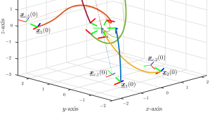
Figure 3: Simulation for five agents in a circular formation.

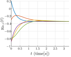
(a) $y_{2c,i}(t)$ for all agents.

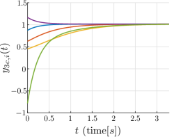
(b) $y_{3c,i}(t)$ for all agents.

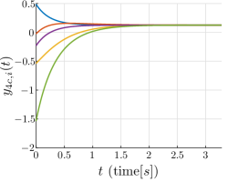
(c) $y_{4c,i}(t)$ for all agents.

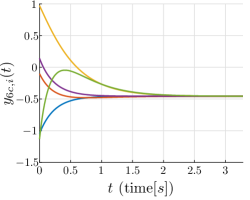
(d) $y_{6c,i}(t)$ for all agents.

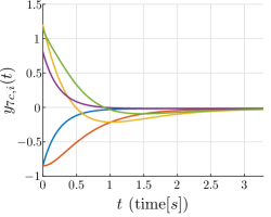
(e) $y_{7c,i}(t)$ for all agents.

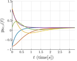
(f) $y_{8c,i}(t)$ for all agents.

Figure 4: Time-evolution for each coefficient of $\underline{\bm{y}}_{c,i}=y_{2c,i}\hat{\imath}+y_{3c,i}\hat{\jmath}+y_{4c,i}\hat{k}+\varepsilon(y_{6c,i}\hat{\imath}+y_{7c,i}\hat{\jmath}+y_{8c,i}\hat{k})$ in the circular formation.

Finally, in order to show scalability and validate the time-varying formation decentralized controller, a second simulation is carried out with 100 agents. First we generate a random fixed directed network containing a directed spanning tree, and then we randomly generate the initial poses $\underline{\bm{x}}_{i}\left(0\right)$, $\forall i\in\left\{1,\ldots,100\right\}$. The random fixed directed network containing a directed spanning tree is obtained according to the following procedure. First we randomly generate a $100\times 100$ matrix and set to zero all elements of the main diagonal. The resulting matrix is defined as the adjacency matrix $\bm{A}$ if the corresponding Laplacian matrix has at most one zero eigenvalue and all the others have positive real part, because such matrix corresponds to a topology that contains a directed spanning tree [1, Cor. 2.5]. If the corresponding Laplacian matrix does not contain at most one zero eigenvalue or has one or more eigenvalues with negative real part, the adjacency matrix is discarded and the procedure is repeated until an appropriate matrix is generated.

The goal is to reach a formation given by

$$\underline{\bm{\delta}}_{i}\left(t\right) =\bm{r}_{x,i}\bm{r}_{z,i}\underline{\bm{p}}\left(t\right),$$ (82)

where $\bm{r}_{z,i}=\bm{r}_{\delta,i}$ as in (79), $\bm{r}_{x,i}=\cos\left(\phi_{\delta,i}/2\right)+\hat{\imath}\sin\left(\phi_{\delta,i}/2\right)$, with $\phi_{\delta,i}$ given by (80), $\underline{\bm{p}}\left(t\right)=1+\varepsilon 0.5\left(-\hat{\imath}-\hat{\jmath}\right)\left(2+\cos\left(8\pi t\right)\right)$ and $\dot{\underline{\bm{p}}}=-\varepsilon 0.5\left(-\hat{\imath}-\hat{\jmath}\right)8\pi\sin\left(8\pi t\right)$, with $t\in[0,0.25]\mathrm{s}$.

(a) $t=0\mathrm{ms}$

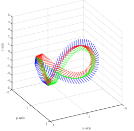
(b) $t=30\mathrm{ms}$

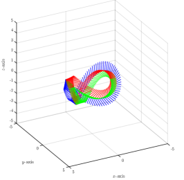
(c) $t=75\mathrm{ms}$

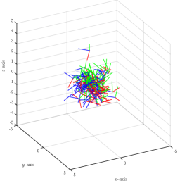
(d) $t=0\mathrm{ms}$

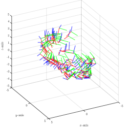
(e) $t=30\mathrm{ms}$

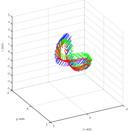
(f) $t=75\mathrm{ms}$

Figure 5: Simulation for 100 agents in a time-varying formation with $\underline{\bm{\delta}}_{i}\left(t\right)$ given by (82). The upper row shows the desired formation and the lower row shows the executed one. From $0\mathrm{ms}$ to $75\mathrm{ms}$, the desired formation is shrinking. When $t=75\mathrm{ms}$, the system has almost achieved the desired formation.

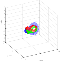
(a) $t=150\mathrm{ms}$

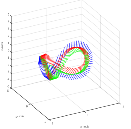
(b) $t=200\mathrm{ms}$

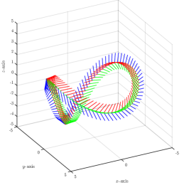
(c) $t=250\mathrm{ms}$

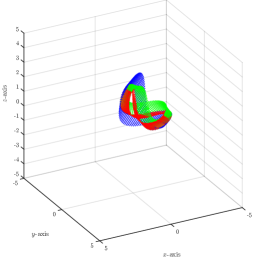
(d) $t=150\mathrm{ms}$

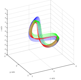
(e) $t=200\mathrm{ms}$

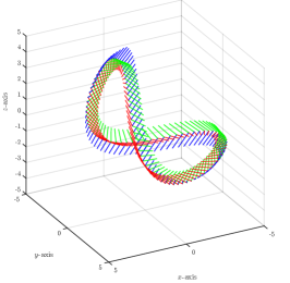
(f) $t=250\mathrm{ms}$

Figure 6: Simulation for 100 agents in a time-varying formation with $\underline{\bm{\delta}}_{i}\left(t\right)$ given by (82). The upper row shows the desired formation and the lower row shows the executed one. From $150\mathrm{ms}$ to $250\mathrm{ms}$, the desired formation is expanding. When $t=150\mathrm{ms}$, the system has already achieved the desired formation and from this point forward it tracks the time-varying formation very closely.

The simulation is shown in Figures 5 and 6. From $0\mathrm{ms}$ to $75\mathrm{ms}$, the desired formation is shrinking, and when $t=75\mathrm{ms}$, the system has almost achieved the desired formation. From $150\mathrm{ms}$ to $250\mathrm{ms}$, the desired formation is expanding, and when $t=150\mathrm{ms}$, the system has already achieved the desired formation. From this point forward it tracks the time-varying formation very closely. This behavior can also be seen in Figure 7, which shows the time evolution of each coefficient of the agents’ outputs. It indicates that after $100\mathrm{ms}$ all agents have agreed on the desired center of formation, which implies that they track the time-varying formation without error. Since the agents agree on a center of formation by means of local information exchange, the formation can happen anywhere in space, as both Figures 5 and 6 show.

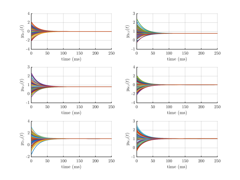
Figure 7: Time-evolution for each coefficient of $\underline{\bm{y}}_{c,i}=y_{2c,i}\hat{\imath}+y_{3c,i}\hat{\jmath}+y_{4c,i}\hat{k}+\varepsilon(y_{6c,i}\hat{\imath}+y_{7c,i}\hat{\jmath}+y_{8c,i}\hat{k})$ when performing the time-varying formation described by (82) and shown in Figures 5 and 6.

6.2 Experiment with two holonomic mobile manipulators

An experimental evaluation is important when proposing new methods that are aimed at being implemented in real multi-robot systems because several real world phenomena are usually disregarded when developing the theory or even in numerical simulations. Some important real issues are actuator saturation, uncertain pose measurements provided by the real sensors, unmodeled dynamics, sampling and quantization errors associated with the discrete implementation, packet loss and time delay related to the real communication infrastructure. Therefore, in this section we present an experiment with actual robots.

It is considered the multi-agent system composed of two mobile manipulators with holonomic base, namely KUKA youBots [45]. These robots are modeled using the whole-body kinematics modeling presented in C. Each robot is equipped with an onboard Mini-ITX computer, with a processor Intel AtomTM Dual Core D510 ($1$M Cache, $2\times 1.66$ GHz), 2GB single-channel DDR2 667MHz memory, 32GB SSD drive, and wireless connection by means of a usb-connected Vonets Wireless Wifi Vap11g card. The experiments were performed at CSAIL, MIT, in a laboratory equipped with a Vicon motion capture system that provides, via wireless communication, the local pose for each robot at 50Hz. The control algorithm was implemented using the Robot Operating System (ROS) and the C++ API of DQ Robotics. ROS is a meta-operating system that provides a structured communications layer fundamentally based on: nodes, which contain the processes performing the computation of robotics algorithms; messages, which are a strictly typed data structure used by nodes to communicate with other nodes; and topics, which are the communication channels used by publisher nodes to send messages and by subscriber nodes to receive messages [46]. This framework makes it easier the task of implementing algorithms in real robotic platforms as it provides a high level hardware abstraction and a set of libraries, drivers, and tools to help the developer.

We have elaborated a collaborative manipulation scenario in which the multi-agent system is composed of the two mobile manipulators and a box to be transported inside the workspace. The formation task is divided in two subtasks. The first one consists of a pre-grasping formation, where the robots gather around a box, which is represented by a static virtual leader, which corresponds to Agent 3 in Figure 8. In the second subtask, the robots grasp the box and move it around the workspace. In this case, the agents have to follow a dynamic virtual leader, as they have to move the box. In both subtasks, the control input for each mobile manipulator is given by (70).

Figure 8: Network topology for the experiment with two mobile manipulators. Nodes 1 and 2 represent each robot, respectively, and node 3 represents the virtual agent (i.e., the box).

The two robots are able to send information to each other and the box acts as a third virtual leader agent providing an output reference related to the desired center of formation. This leader is an agent that provides information without listening to other agents and without executing the consensus protocol to update the output reference. The whole system is modeled by the network topology shown in Figure 8, where node 3 is the virtual agent used to generate the reference for the desired formation, and nodes 1 and 2 are the mobile manipulators. By using that topology, Agent 3 provides the reference about the desired center of formation only to Agent 1.

We use a Multi-Master ROS architecture [47] to implement a distributed architecture. This is shown in Figure 9, where the gray circles refer to the nodes running on each independent agent and the square white boxes are the shared topics, which are the communication channels in the ROS architecture. In one fixed computer, which is responsible for the localization system, the poses of the agents’ bases, namely pose_base_1 and pose_base_2, are provided by the Vicon motion capture system and made available through ROS topics that any agent on the system can have access. Furthermore, this same computer is responsible for the role of the virtual Agent 3 (the box), providing information about the center of formation, output_pose_3, as well as providing the information for every agent about their relative pose $\underline{\bm{\delta}}_{i}$ with respect to the center of formation, namely relative_pose_1 and relative_pose_2. Separately, each agent runs its own ROS master and shares topics with the agents and the fixed computer using the Multi-Master ROS architecture. Each agent is able to access its own local information regarding its end-effector pose and also its formation parameter $\underline{\bm{\delta}}_{i}$, which is provided by the fixed computer. Furthemore, the agents exchange data with their neighbors—more specifically output_pose_1, output_pose_2 and output_pose_3—according to the graph topology shown in Figures 8 and 9.

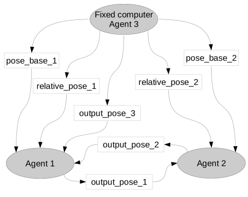
Figure 9: Multi-master ROS architecture with shared topics.

6.2.1 Pre-grasping formation

The first goal is to achieve formation around a box, whose location is informed by the state of agent $3$. For this first task, the relative pose $\underline{\bm{\delta}}_{i}$ of each agent (i.e., the pose of each end-effector with respect to the center of formation) is defined such that the end-effectors of agents $1$ and $2$ should point to the center of formation at a distance of 0.30 m in the $x$ axis in opposite directions; that is,

$$\underline{\bm{\delta}}_{1}=1-\varepsilon 0.15\hat{\imath}$$ (83)

and

$$\underline{\bm{\delta}}_{2}=\hat{k}\left(1-\varepsilon 0.15\hat{\imath}\right).$$ (84)

The initial configuration of the experiment is shown in Figure 10a, which shows the two KUKA YouBots. Agent $1$ corresponds to the robot in the left, agent $2$ corresponds to the robot in the right, and the virtual agent $3$ corresponds to the box. The Laplacian matrix is thus given by

$$\bm{L} =\begin{bmatrix}1&-0.5&-0.5\\ -0.5&0.5&0\\ 0&0&0\end{bmatrix},$$ (85)

where the weights of all edges were chosen as 0.5 after a process of trial and error, throughout several executions, in order to achieve satisfactory convergence rate.

During the execution of the experiment, as shown in Figures 10b, 10c, and finally Figure 10d, the agents are able to achieve formation around the box with the desired poses given by $\underline{\bm{\delta}}_{1}$ and $\underline{\bm{\delta}}_{2}$, relative to the center of formation, which is located at the center of the box.

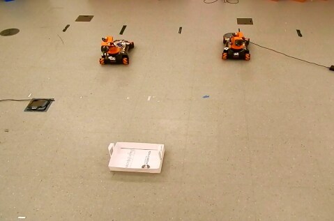
(a) $t=0$s.

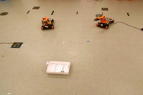
(b) $t=1$s.

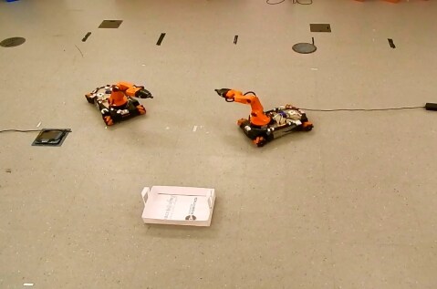
(c) $t=3$s.

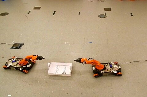
(d) $t=14$s.

Figure 10: Experiment on formation control with two KUKA YouBots. The goal is to have a final formation where the robots are located around the box with their end-effectors pointing to the center of the box, opposite to each other.

The state trajectories of the outputs $\underline{\bm{y}}_{ce,i}=y_{ce,i,2}\hat{\imath}+y_{ce,i,3}\hat{\jmath}+y_{ce,i,4}\hat{k}+\varepsilon(y_{ce,i,6}\hat{\imath}+y_{ce,i,7}\hat{\jmath}+y_{ce,i,8}\hat{k})$ for each agent are shown in Figure 11. The constant yellow line represents the leader state (i.e., the box pose), and the blue and orange lines represent agents $1$ and $2$, respectively. The continuous lines represent the measurements of the agents outputs, and the thinner dashed lines represent the solution given by a simulation carried out with the same initial pose configurations. The states mainly follow the expected behavior given by the analytical solution, although noises, delays, and initial conditions on velocities, which are not explicitly considered in the designed control laws, cause some deviations from the simulated values, as expected.

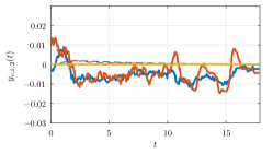
(a) $y_{ce,i,2}(t)$ for each agent.

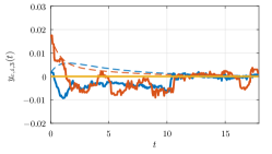
(b) $y_{ce,i,3}(t)$ for each agent.

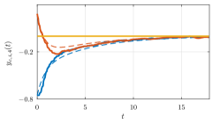
(c) $y_{ce,i,4}(t)$ for each agent.

(d) $y_{ce,i,6}(t)$ for each agent.

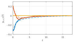
(e) $y_{ce,i,7}(t)$ for each agent.

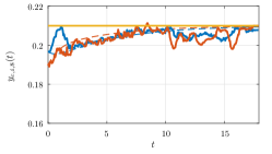
(f) $y_{ce,i,8}(t)$ for each agent.

Figure 11: Coefficients of the output $\underline{\bm{y}}_{ce,i}$ of each agent in the experiment on formation with two KUKA YouBots. The dashed curves correspond to the simulated values, whereas the solid ones correspond to the actual values obtained from the experiments. The constant curves correspond to the reference provided by the virtual agent 3.

6.2.2 Cooperative manipulation

In this second subtask, the goal is to make the robots grasp the box and then move it around the workspace while maintaining the formation. To that end, after the robots achieve the formation around the box in the pre-grasping subtask, as shown in Figure 10d, the references $\underline{\bm{\delta}}_{i}$ are changed to a lower position in the $z$ axis and rotated around the $y$ axis, so that the agents adjust the grasp (Figure 12a). By reducing the distance of each $\underline{\bm{\delta}}_{i}$ with respect to the center of formation and returning the reference to a higher position in the $z$ axis, the agents grasp the box by the flexible straps (Figure 12b). Next, the reference corresponding to the box location is changed in order to drive the agents to a pick up zone, where the box is loaded (Figure 12c). After loading the box in the pick-up zone, the reference is changed again and the agents carry the box in the direction of a delivery zone, passing through the location shown in Figure 12d, then reaching the delivery zone in Figure 12e. Once the agents reach the delivery zone, the value of each $\underline{\bm{\delta}}_{i}$ is changed in order to release and deliver the box (Figure 12f).

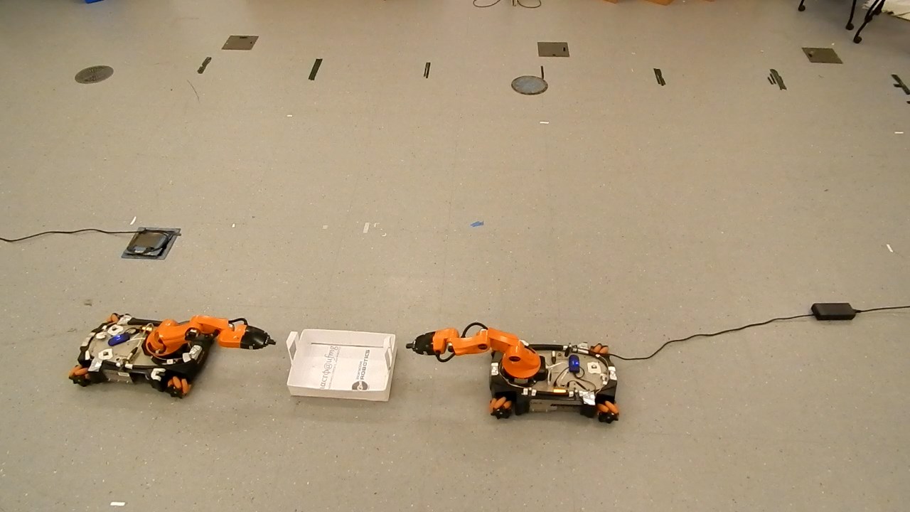
(a) Adjusting the grasp.

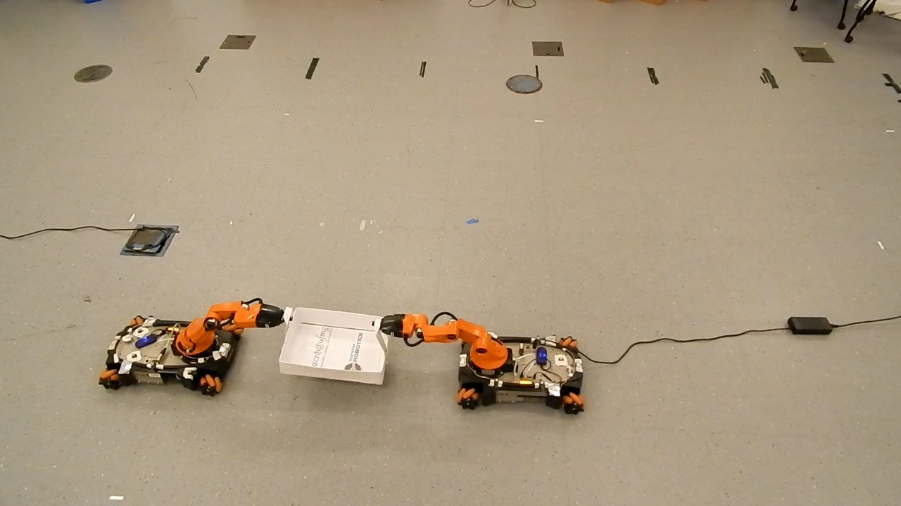
(b) Carrying the box.

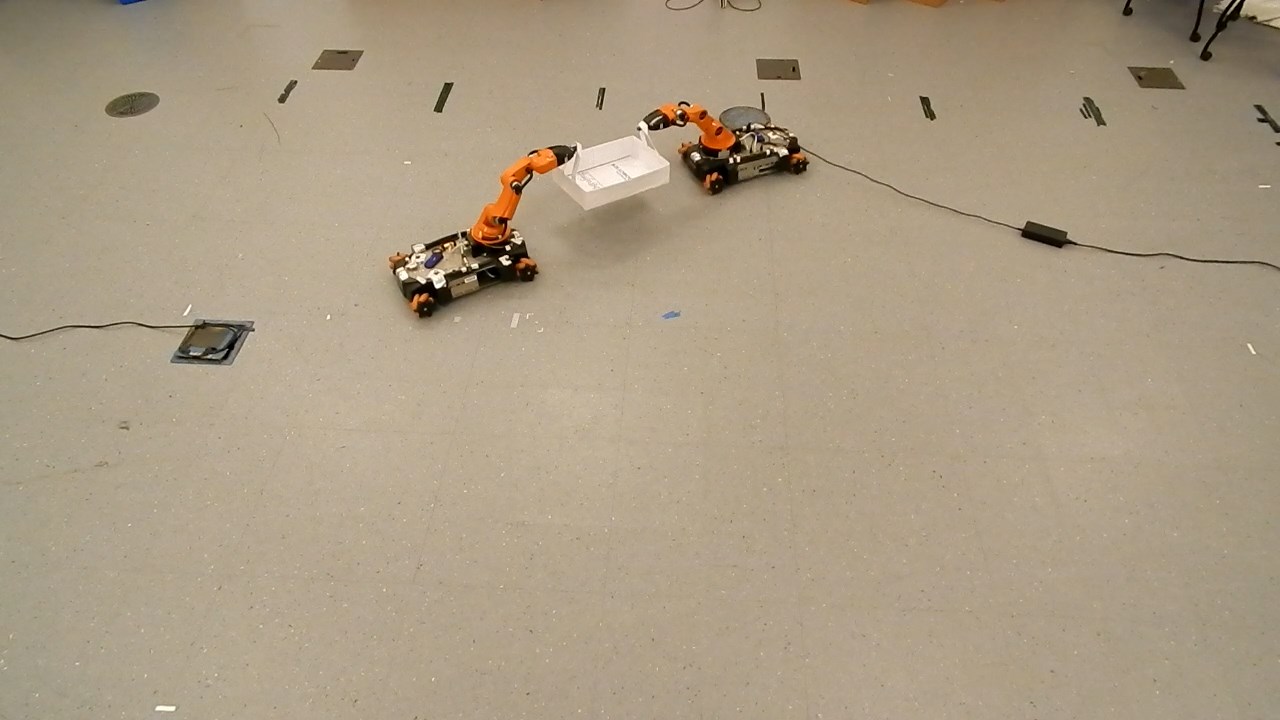
(c) Pick-up zone.

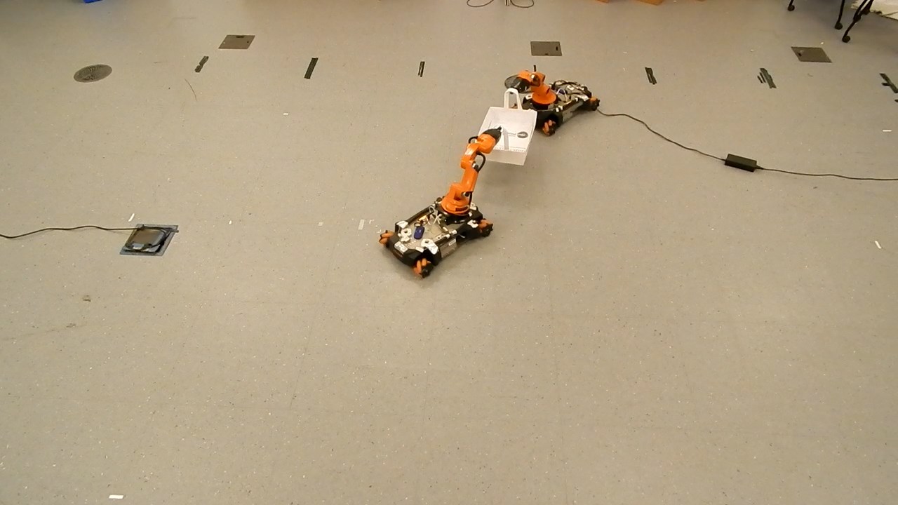
(d) Carrying the box to the delivery zone.

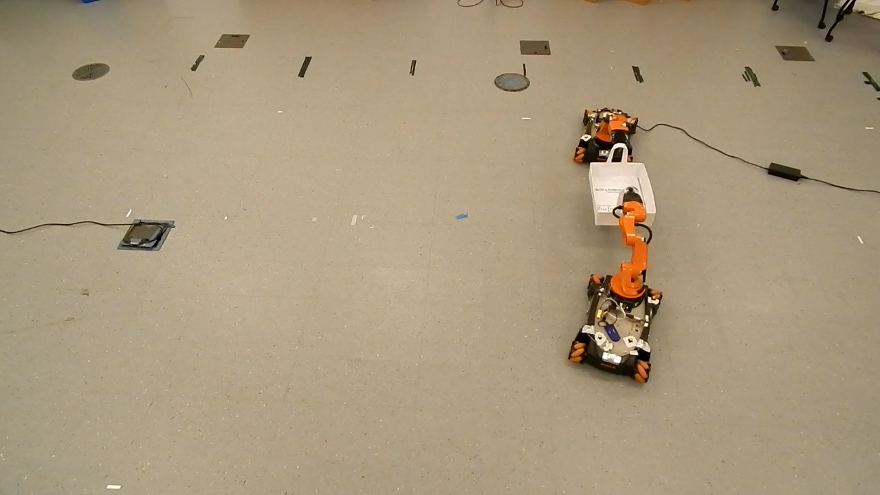
(e) Delivery zone.

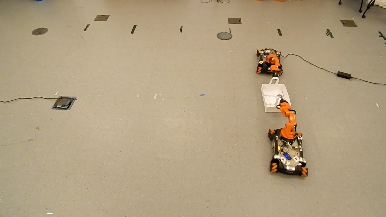
(f) Delivering the box.

Figure 12: Experiment on cooperative manipulation with KUKA YouBots.

With the interplay between changing the reference of an object, which is represented by Agent $3$, and providing different assignments of $\underline{\bm{\delta}}_{i}$ for each robot, many different tasks can be achieved, as depicted in the given example.

6.2.3 Discussion

The manipulation task presented in this section can be categorized as a leader-following problem as we have defined the pose of the box as a single virtual leader. Although we have not explicitly mentioned the solution of this type of problem in the development of our theoretical results, the techniques proposed in this work are general enough to allow its treatment. More specifically, when a single virtual leader is static, the leader-following problem can also be defined as a consensus regulation problem in which the objective is to guide the consensus variables of the system to the values of the leader variables, in contrast to the leaderless consensus problem, where the variables converge to a set of values that are a function of the initial values of the agents variables. Therefore, as the first subtask consists of a pre-grasping formation, where the robots gather around a box, which is represented by a static virtual leader (Agent 3 in Figure 8), the leader-following problem boils down to a consensus regulation problem with a static leader as the root of a directed spanning tree, thus satisfying the requirement of the existence of a directed spanning tree stated in our proofs. In conclusion, the execution of this subtask can be seen as a real world verification of the proposed methodology.

On the other hand, in the second subtask, the robots grasp the box and move it around the workspace. In this case, the agents have to follow a dynamic virtual leader, as they have to move the box. Although the design of controllers able to guarantee perfect tracking of a dynamic leader is out of the scope of this work, by designing a trajectory in which the virtual leader moves smoothly and slowly enough, the system has shown to be able to track it with a small error. Indeed, this demonstrates some robustness of our approach as the independent dynamic behavior of the leader can be seen as a disturbance to the system.

7 Conclusion

This paper presented a solution based on dual quaternion algebra to the general problem of pose consensus for systems composed of multiple rigid-bodies, and then extended the theory in order to design consensus-based formation control laws. Since unit dual quaternions belong to a non-Euclidean manifold, the consensus protocols usually found in the literature cannot be directly applied to the problem of pose consensus because those protocols assume an $n$-dimensional Euclidean space. However, thanks to the isomorphism of pure dual quaternions (i.e., dual quaternions with real part equal to zero) and $\mathbb{R}^{6}$ under the addition operation, an output consensus protocol was designed and then we proved that output consensus (i.e., consensus on $\log{\underline{\bm{x}}}_{i}$) implies pose consensus (i.e., consensus on $\underline{\bm{x}}_{i}$). This result, together with the differential logarithm mapping of unit dual quaternions, allowed the design of pose consensus protocols, which ensures that the system will achieve consensus as long as the information flow is described by directed graphs that have a directed spanning tree.

Since dual quaternions are a generalization of quaternions, the corresponding proofs are much more compact than those obtained when using quaternions. Usually, proofs are shorter because we do not need to do a separate analysis for rotation and translation, and, in addition, we usually exploit the dual quaternion algebra to make those proofs even cleaner and shorter.

Furthermore, unit dual quaternions capture the intrinsic coupling between translation and rotation in rigid motions, which has an important practical consequence: the instantaneous control effort (i.e., the norm of the control input) of controllers based on dual quaternions is smaller than the instantaneous control effort of decoupled controllers that use rotation quaternions and translation vectors separately, as reported in the literature [48].

A consensus-based approach for formation control of free-flying rigid-body teams was also proposed and then applied to the decentralized formation control of mobile manipulators. In that case, the objective is to achieve desired formations for the set of end-effectors of mobile manipulators and let each robot generate its own motion in order to move the end-effector according to the reference provided by the consensus protocol. The advantage of using such abstraction is that the consensus protocols are used to determine, in a decentralized way, how each robot’s end-effector should be, regardless of the topology and dimension of the robots’ configuration spaces. In fact, since the robots use local motion controllers, the consensus-based formation control can be applied to a highly heterogeneous multi-agent system as long as each agent is capable of following the reference provided by the consensus protocols.

Finally, numerical simulations were carried out to illustrate the applicability and scalability of the proposed method and an experiment with real mobile manipulators was presented to show the proposed method, in practice, in a cooperative manipulation scenario.

Although the proposed distributed control laws ensure consensus of free-flying agents, we have not taken into account the problem of unwinding. As a result, agents may execute longer trajectories before the overall system achieves consensus. Future works will be focused on the unwinding problem in the context of pose consensus protocols, which can only be solved by using discontinuous or hybrid controllers [36], and may also take into account time-delays in the agents interactions, switching topologies, leader-follower with multiple dynamic leaders, containment control, and couplings design.

Appendix A Auxiliary facts and proofs

Fact 16.

Given $\bm{y}=\left(\phi/2\right)\bm{n}$, where $\bm{n}\in\mathbb{S}^{3}\cap\mathbb{H}_{p}$ and $\phi\in\left[0,2\pi\right)$,

$$\frac{\cos\left\|\bm{y}\right\|}{\left\|\bm{y}\right\|^{m}} =\frac{\cos\left(\phi/2\right)}{\left(\phi/2\right)^{m}}$$ (i)

$$\frac{\sin\left\|\bm{y}\right\|}{\left\|\bm{y}\right\|^{m}} =\frac{\sin\left(\phi/2\right)}{\left(\phi/2\right)^{m}}.$$ (ii)

Proof.

Since $\left\|\bm{n}\right\|=1$, then $\left\|\bm{y}\right\|=\left|\phi\right|/2=\phi/2$ because $\phi$ is nonnegative. Thus we obtain (i) and (ii). ∎

Proposition 17.

Let $\bm{A}\in\mathbb{R}^{m\times n}$, $\bm{x}\in\mathbb{R}^{n}$, and $\bm{b}\in\mathbb{R}^{m}$ such that

$$\bm{A}\bm{x}=\bm{b}$$ (86)

and $m\geq n$. If there exists a left pseudoinverse $\bm{A}^{+}$ such that $\bm{A}^{+}\bm{A}=\bm{I}$, then the solution to (86) given by $\bm{x}=\bm{A}^{+}\bm{b}$ is unique and $\bm{b}=\bm{0}$ if and only if $\bm{x}=\bm{0}$.

Proof.

If there exists $\bm{A}^{+}$ such that $\bm{A}^{+}\bm{A}=\bm{I}$ then $\bm{A}\bm{A}^{+}\bm{A}=\bm{A}$, thus $\bm{b}=\bm{A}\bm{x}=\bm{A}\bm{A}^{+}\bm{A}\bm{x}=\bm{A}\bm{A}^{+}\bm{b}$. This way, $\bm{x}=\bm{A}^{+}\bm{b}$ is clearly a solution to (86) because $\bm{A}\bm{x}=\bm{A}\bm{A}^{+}\bm{b}=\bm{b}$. Furthermore, suppose that $\bm{x}^{\prime}$ is also a solution to (86), thus $\bm{b}=\bm{A}\bm{x}^{\prime}=\bm{A}\bm{x}$. Since $\bm{A}^{+}\bm{A}=\bm{I}$ then $\bm{A}^{+}\bm{A}\bm{x}^{\prime}=\bm{A}^{+}\bm{A}\bm{x}$ implies $\bm{x}^{\prime}=\bm{x}$, hence $\bm{x}=\bm{A}^{+}\bm{b}$ is indeed a unique solution.

Lastly, if $\bm{x}=\bm{0}$ then $\bm{b}=\bm{A}\bm{x}=\bm{A}\bm{0}=\bm{0}$; conversely, if $\bm{b}=\bm{0}$ then $\bm{x}=\bm{A}^{+}\bm{b}=\bm{A}^{+}\bm{0}=\bm{0}$. Hence $\bm{b}=\bm{0}\iff\bm{x}=\bm{0}$. ∎

Proposition 18.

Consider $\bm{r}\in\mathbb{S}^{3},$ with $\bm{r}=\cos\left(\phi/2\right)+\bm{n}\sin\left(\phi/2\right)$ and $\bm{n}\in\mathbb{S}^{3}\cap\mathbb{H}_{p}$, and $\bm{y}\in\mathbb{H}_{p}$ such that $\bm{y}\triangleq\log\bm{r}$, then

$$\bm{Q}\left(\bm{r}\right)\triangleq\frac{\partial\operatorname{vec}_{4}\bm{r}}{\partial\operatorname{vec}_{3}\bm{y}}$$

is full column rank for $\phi\in\left[0,2\pi\right)$.

Proof.

$\bm{Q}\left(\bm{r}\right)$ is full column rank if $\det\left(\bm{Q}\left(\bm{r}\right)^{T}\bm{Q}\left(\bm{r}\right)\right)\neq 0$. Thus,

$$\det\left(\bm{Q}\left(\bm{r}\right)^{T}\bm{Q}\left(\bm{r}\right)\right)=\Theta^{4}\sin^{2}\left(\frac{\phi}{2}\right)\left(n_{x}^{2}+n_{y}^{2}+n_{z}^{2}\right)\\ +\Gamma^{2}\Theta^{4}\left(n_{x}^{4}+n_{y}^{4}+n_{z}^{4}+2n_{x}^{2}n_{y}^{2}+2n_{x}^{2}n_{z}^{2}+2n_{y}^{2}n_{z}^{2}\right)\\ +2\Gamma\Theta^{5}\left(n_{x}^{2}+n_{y}^{2}+n_{z}^{2}\right)+\Theta^{6},$$

where $\Gamma$ and $\Theta$ are defined as in Theorem 2. Using the fact that $\left\|\bm{n}\right\|=1$, $\Gamma=r_{1}-\Theta$ and

$$\left(n_{x}^{2}+n_{y}^{2}+n_{z}^{2}\right)^{2} =n_{x}^{4}+n_{y}^{4}+n_{z}^{4}+2n_{x}^{2}n_{y}^{2}+2n_{x}^{2}n_{z}^{2}+2n_{y}^{2}n_{z}^{2},$$

we obtain

$$\det\left(\bm{Q}\left(\bm{r}\right)^{T}\bm{Q}\left(\bm{r}\right)\right) =\Theta^{4}\sin^{2}\left(\frac{\phi}{2}\right)+\Gamma^{2}\Theta^{4}+2\Gamma\Theta^{5}+\Theta^{6}$$

$$=\Theta^{4}\left(\sin^{2}\left(\frac{\phi}{2}\right)+\Gamma^{2}+2\Gamma\Theta+\Theta^{2}\right)$$

$$=\Theta^{4},$$

which is different from zero for $\phi\in\left[0,2\pi\right)$. ∎

Proposition 19.

Given $\bm{p}\in\mathbb{H}_{p}$ and $\bm{r}\in\mathbb{S}^{3}$, the inverse of

$$\bm{A}=\begin{bmatrix}\bm{I}_{4}&\bm{0}_{4\times 4}\\ \frac{1}{2}\overset{+}{\bm{H}}_{4}\left(\bm{p}\right)&\overset{-}{\bm{H}}_{4}\left(\bm{r}\right)\end{bmatrix}$$

is given by

$$\bm{A}^{-1}=\begin{bmatrix}\bm{I}_{4}&\bm{0}_{4\times 4}\\ -\frac{1}{2}\overset{-}{\bm{H}}_{4}\left(\bm{r}^{*}\right)\overset{+}{\bm{H}}_{4}\left(\bm{p}\right)&\overset{-}{\bm{H}}_{4}\left(\bm{r}^{*}\right)\end{bmatrix}.$$

Proof.

Since $\overset{-}{\bm{H}}_{4}\left(\bm{r}^{*}\right)=\overset{-}{\bm{H}}_{4}\left(\bm{r}\right)^{T}$ and $\overset{-}{\bm{H}}_{4}\left(\bm{r}\right)\in\mathrm{O}\left(4\right)$ by Propositions 20 and 21, the result $\bm{A}\bm{A}^{-1}=\bm{A}^{-1}\bm{A}=\bm{I}_{8}$ follows by direct calculation. ∎

Appendix B Facts about Hamilton operators

Proposition 20.

Let $\bm{h}\in\mathbb{H}$, $\overset{-}{\bm{H}}_{4}\left(\bm{h}^{*}\right)=\overset{-}{\bm{H}}_{4}\left(\bm{h}\right)^{T}$ and $\overset{+}{\bm{H}}_{4}\left(\bm{h}^{*}\right)=\overset{+}{\bm{H}}_{4}\left(\bm{h}\right)^{T}$.

Proof.

Since the Hamilton operators $\overset{+}{\bm{H}}$ and $\overset{-}{\bm{H}}$ are defined as in (12), these equalities can be verified by inspection. ∎

Proposition 21.

If $\bm{r}\in\mathbb{S}^{3}$ then $\overset{+}{\bm{H}}_{4}\left(\bm{r}\right),\overset{-}{\bm{H}}_{4}\left(\bm{r}\right)\in\mathrm{O}\left(4\right)$.

Proof.

Since $\bm{r}\in\mathbb{S}^{3}$ then $\bm{r}^{*}\bm{r}=1$ and $\bm{x}=\bm{x}\bm{r}^{*}\bm{r}$, $\forall\bm{x}\in\mathbb{H}$, which implies

$$\operatorname{vec}_{4}\bm{x} =\overset{-}{\bm{H}}_{4}\left(\bm{r}\right)\operatorname{vec}_{4}\left(\bm{x}\bm{r}^{*}\right)$$

$$=\overset{-}{\bm{H}}_{4}\left(\bm{r}\right)\overset{-}{\bm{H}}_{4}\left(\bm{r}^{*}\right)\operatorname{vec}_{4}\bm{x}$$

$$=\overset{-}{\bm{H}}_{4}\left(\bm{r}^{*}\bm{r}\right)\operatorname{vec}_{4}\bm{x},\qquad\forall\operatorname{vec}_{4}\bm{x}\in\mathbb{R}^{4}.$$

Thus $\overset{-}{\bm{H}}_{4}\left(\bm{r}\right)\overset{-}{\bm{H}}_{4}\left(\bm{r}^{*}\right)=\overset{-}{\bm{H}}_{4}\left(\bm{r}^{*}\bm{r}\right)=\bm{I}$, therefore $\overset{-}{\bm{H}}_{4}\left(\bm{r}^{*}\right)=\overset{-}{\bm{H}}_{4}\left(\bm{r}\right)^{-1}$. Furthermore, from Proposition 20 we have that $\overset{-}{\bm{H}}_{4}\left(\bm{r}^{*}\right)=\overset{-}{\bm{H}}_{4}\left(\bm{r}\right)^{T}$, which implies $\overset{-}{\bm{H}}_{4}\left(\bm{r}\right)^{-1}=\overset{-}{\bm{H}}_{4}\left(\bm{r}\right)^{T}$ and hence $\overset{-}{\bm{H}}_{4}\left(\bm{r}\right)\in\mathrm{O}\left(4\right)$.

From $\bm{x}=\bm{r}^{*}\bm{r}\bm{x}$, $\forall\bm{x}\in\mathbb{H}$, we apply the same reasoning to conclude that $\overset{+}{\bm{H}}_{4}\left(\bm{r}\right)\in\mathrm{O}\left(4\right)$. ∎

Appendix C Whole Body Kinematics of Holonomic Mobile Manipulators

Consider a holonomic mobile base moving in the plane $XY$ and an inertial reference frame $\mathcal{F}_{0}$ somewhere in the space. The position of the local reference frame $\mathcal{F}_{b}$ in the center of the mobile base is given by the coordinates $\left(x,y\right)$, and the orientation is given by the rotation angle $\phi$ around axis $Z$. Thus, the generalized coordinates of the base can be written as $\bm{q}_{b}=\begin{bmatrix}x&y&\phi\end{bmatrix}^{T}$ and its pose, relative to $\mathcal{F}_{0}$, is given by the following dual quaternion

$$\underline{\bm{x}}_{b}^{0}=\bm{r}_{b}^{0}+\varepsilon\frac{1}{2}\bm{p}_{0,b}^{0}\bm{r}_{b}^{0},$$ (87)

where $\bm{r}_{b}^{0}=\cos\left(\phi/2\right)+\hat{k}\sin\left(\phi/2\right)$ and $\bm{p}_{0,b}^{0}=x\hat{\imath}+y\hat{\jmath}$ [31].

Taking the first time-derivative of (87) and mapping into $\mathbb{R}^{8}$ with the $\operatorname{vec}_{8}$ operator, the differential forward kinematics of the holonomic mobile base is given by

$$\operatorname{vec}_{8}\dot{\underline{\bm{x}}}_{b}^{0}=\bm{J}_{b}\dot{\bm{q}}_{b},$$ (88)

where $\bm{J}_{b}$ is the (dual quaternion) Jacobian matrix (see page 89 in [31]).

Next, consider a manipulator on top of the mobile base. Let the reference frame of the manipulator’s base be $\mathcal{F}_{m}$ and $\underline{\bm{x}}_{m}^{b}$ be a constant dual quaternion representing the rigid-motion from $\mathcal{F}_{b}$ to $\mathcal{F}_{m}$. For a serial manipulator with $\eta$ revolute joints, with $\theta_{k}$ being the angle of the $k$-th joint, for $k=1,\ldots,\eta$, the forward kinematics that relates the frame $\mathcal{F}_{e}$ of the end-effector to the base of the manipulator $\mathcal{F}_{m}$ is a function of all joints. More specifically, the pose of the end-effector with respect to the base of the manipulator is given by the unit dual quaternion $\underline{\bm{x}}_{e}^{m}=\underline{\bm{f}}(\bm{q}_{m})$, with $\bm{q}_{m}=\begin{bmatrix}\theta_{1}&\cdots&\theta_{\eta}\end{bmatrix}^{T}$ being the vector containing all the joint angles [31].

The differential forward kinematics is given by $\dot{\underline{\bm{x}}}_{e}^{m}=\underline{\bm{f}}^{\prime}(\bm{q}_{m})$, where $\underline{\bm{f}}^{\prime}\triangleq d\underline{\bm{f}}/dt$. Thus, applying the $\operatorname{vec}_{8}$ operator, the differential forward kinematics of the manipulator is

$$\operatorname{vec}_{8}\dot{\underline{\bm{x}}}_{e}^{m}=\bm{J}_{m}\dot{\bm{q}}_{m},$$ (89)

where $\bm{J}_{m}=\partial\underline{\bm{f}}/\partial\theta_{m}\in\mathbb{R}^{8\times\eta}$ is the analytical Jacobian relating the joints velocities to the derivative of the unit dual quaternion that represents the end-effector pose. Notice that both forward kinematics and differential forward kinematics are obtained directly in the algebra of dual quaternions [31].

Coupling the manipulator to the mobile base, the pose of the end-effector, related to the inertial coordinate frame $\mathcal{F}_{0}$, is described by the composition of each subsystem and its time derivative is given by

$$\underline{\bm{x}}_{e}^{0}=\underline{\bm{x}}_{b}^{0}\underline{\bm{x}}_{m}^{b}\underline{\bm{x}}_{e}^{m}\implies\dot{\underline{\bm{x}}}_{e}^{0}=\dot{\underline{\bm{x}}}_{b}^{0}\underline{\bm{x}}_{m}^{b}\underline{\bm{x}}_{e}^{m}+\underline{\bm{x}}_{b}^{0}\underline{\bm{x}}_{m}^{b}\dot{\underline{\bm{x}}}_{e}^{m}.$$ (90)

Mapping (90) into $\mathbb{R}^{8}$, and using (11), (88), and (89), we obtain which can be written as

$$\operatorname{vec}_{8}\dot{\underline{\bm{x}}}_{e}^{0} =\overset{-}{\bm{H}}_{8}(\underline{\bm{x}}_{m}^{b}\underline{\bm{x}}_{e}^{m})\bm{J}_{b}\dot{\bm{q}}_{b}+\overset{+}{\bm{H}}_{8}(\underline{\bm{x}}_{b}^{0}\underline{\bm{x}}_{m}^{b})\bm{J}_{m}\dot{\bm{q}}_{m},$$ (91)

$$=\bm{J}_{w}\dot{\bm{q}}_{w},$$ (92)

where

$$\bm{J}_{w}=\begin{bmatrix}\overset{-}{\bm{H}}_{8}(\underline{\bm{x}}_{m}^{b}\underline{\bm{x}}_{e}^{m})\bm{J}_{b}&&\overset{+}{\bm{H}}_{8}(\underline{\bm{x}}_{b}^{0}\underline{\bm{x}}_{m}^{b})\bm{J}_{m}\end{bmatrix}$$ (93)

and $\dot{\bm{q}}_{w}=\begin{bmatrix}\dot{\bm{q}}_{b}\\ \dot{\bm{q}}_{m}\end{bmatrix}$.

References

References

• [1] W. Ren and R. W. Beard, Distributed consensus in multi-vehicle cooperative control.   Springer-Verlag, London, U.K., 2008.
• [2] K.-K. Oh, M.-C. Park, and H.-S. Ahn, “A survey of multi-agent formation control,” Automatica, vol. 53, pp. 424–440, 2015.
• [3] M. A. Arteaga–Pérez and E. Nuño, “Velocity observer design for the consensus in delayed robot networks,” Journal of the Franklin Institute, vol. 355, no. 14, pp. 6810 – 6829, 2018.
• [4] T. Hatanaka, N. Chopra, M. Fujita, and M. W. Spong, Passivity-Based Control and Estimation in Networked Robotics.   Communications and Control Engineering Series, Springer-Verlag, 2015.
• [5] Y. Cao, W. Yu, W. Ren, and G. Chen, “An overview of recent progress in the study of distributed multi-agent coordination,” IEEE Transactions on Industrial Informatics, vol. 9, no. 1, pp. 427–438, 2013.
• [6] T. Vicsek, A. Czirók, E. B. Jacob, I. Cohen, and O. Schochet, “Novel type of phase transitions in a system of self-driven particles,” Physical Review Letters, vol. 75, no. 6, pp. 1226–1229, 1995.
• [7] J. A. Fax and R. M. Murray, “Graph laplacians and stabilization of vehicle formations,” in Proceedings of the 15th IFAC World Congress, Barcelona, Spain, 2002, pp. 283–288.
• [8] A. Jadbabaie, J. Lin, and A. S. Morse, “Coordination of groups of mobile autonomous agents using nearest neighbor rules,” IEEE Transactions on Automatic Control, vol. 48, no. 6, pp. 988–1001, 2003.
• [9] M. Schwager, N. Michael, V. Kumar, and D. Rus, “Time scales and stability in networked multi-robot systems,” in IEEE International Conference on Robotics and Automation (ICRA), Shanghai, China, 2011, pp. 3855–3862.
• [10] H. Bai and J. T. Wen, “Cooperative load transport: a formation-control perspective,” IEEE Transactions on Robotics, vol. 26, no. 4, pp. 742–750, 2010.
• [11] L. Brinón-Arranz, A. Seuret, and C. Canudas-de Wit, “Cooperative control design for time-varying formations of multi-agent systems,” IEEE Transactions on Automatic Control, vol. 59, no. 8, pp. 2283–2288, 2014.
• [12] R. Wang, X. Dong, Q. Li, and Z. Ren, “Distributed adaptive time-varying formation for multi-agent systems with general high-order linear time-invariant dynamics,” Journal of the Franklin Institute, vol. 353, no. 10, pp. 2290–2304, 2016.
• [13] Y. Zhao, Q. Duan, G. Wen, D. Zhang, and B. Wang, “Time-Varying Formation for General Linear Multiagent Systems Over Directed Topologies: A Fully Distributed Adaptive Technique,” IEEE Transactions on Systems, Man, and Cybernetics: Systems, vol. PP, pp. 1–10, 2018. [Online]. Available: https://ieeexplore.ieee.org/document/8532129/
• [14] X. Li and L. Xie, “Dynamic Formation Control Over Directed Networks Using Graphical Laplacian Approach,” IEEE Transactions on Automatic Control, vol. 63, no. 11, pp. 3761–3774, nov 2018. [Online]. Available: https://ieeexplore.ieee.org/document/8270712/
• [15] Z. Li, W. Ren, X. Liu, and M. Fu, “Distributed containment control of multi-agent systems with general linear dynamics in the presence of multiple leaders,” International Journal of Robust and Nonlinear Control, vol. 23, no. 5, pp. 534–547, mar 2013. [Online]. Available: http://doi.wiley.com/10.1002/rnc.1847
• [16] X. Dong and G. Hu, “Time-varying formation tracking for linear multiagent systems with multiple leaders,” IEEE Transactions on Automatic Control, vol. 62, no. 7, pp. 3658–3664, 2017.
• [17] X. Dong, Y. Hua, Y. Zhou, Z. Ren, and Y. Zhong, “Theory and Experiment on Formation-Containment Control of Multiple Multirotor Unmanned Aerial Vehicle Systems,” IEEE Transactions on Automation Science and Engineering, vol. 16, no. 1, pp. 229–240, jan 2019. [Online]. Available: https://ieeexplore.ieee.org/document/8295262/
• [18] J.-L. Wang and H.-N. Wu, “Leader-following formation control of multi-agent systems under fixed and switching topologies,” International Journal of Control, vol. 85, no. 6, pp. 695–705, jun 2012. [Online]. Available: http://www.tandfonline.com/doi/abs/10.1080/00207179.2012.662720
• [19] X. Dong and G. Hu, “Time-varying formation control for general linear multi-agent systems with switching directed topologies,” Automatica, vol. 73, pp. 47–55, 2016.
• [20] Y. Hua, X. Dong, J. Wang, Q. Li, and Z. Ren, “Time-varying output formation tracking of heterogeneous linear multi-agent systems with multiple leaders and switching topologies,” Journal of the Franklin Institute, vol. 356, no. 1, pp. 539–560, jan 2019. [Online]. Available: https://doi.org/10.1016/j.jfranklin.2018.11.006https://linkinghub.elsevier.com/retrieve/pii/S0016003218306720
• [21] X. Dong, Q. Li, Z. Ren, and Y. Zhong, “Formation-containment control for high-order linear time-invariant multi-agent systems with time delays,” Journal of the Franklin Institute, vol. 352, no. 9, pp. 3564–3584, 2015.
• [22] J. Yu, X. Dong, Q. Li, and Z. Ren, “Robust ${H}\infty$ Guaranteed Cost Time-Varying Formation Tracking for High-Order Multiagent Systems With Time-Varying Delays,” IEEE Transactions on Systems, Man, and Cybernetics: Systems, vol. PP, pp. 1–11, 2018. [Online]. Available: https://ieeexplore.ieee.org/document/8587143/
• [23] H. J. Savino, R. P. dos Santos, C, F. O. Souza, L. C. A. Pimenta, M. de Oliveira, and R. M. Palhares, “Conditions for consensus of multi-agent systems with time-delays and uncertain switching topology,” IEEE Transactions on Industrial Electronics, vol. 63, no. 2, pp. 1258–1267, 2016.
• [24] C. G. Mayhew, R. G. Sanfelice, J. Sheng, M. Arcak, and A. R. Teel, “Quaternion-based hybrid feedback for robust global attitude synchronization,” IEEE Transactions on Automatic Control, vol. 57, no. 8, pp. 2122–2127, 2012.
• [25] A. Sarlette, R. Sepulchre, and N. E. Leonard, “Autonomous rigid body attitude synchronization,” Automatica, vol. 45, no. 2, pp. 572 – 577, 2009.
• [26] C. I. Aldana, E. Romero, E. Nuño, and L. Basañez, “Pose consensus in networks of heterogeneous robots with variable time delays,” International Journal of Robust and Nonlinear Control, vol. 25, no. 14, pp. 2279–2298, 2015.
• [27] C. I. Aldana, E. Nuño, L. Basañez, and E. Romero, “Operational space consensus of multiple heterogeneous robots without velocity measurements,” Journal of the Franklin Institute, vol. 351, no. 3, pp. 1517 – 1539, 2014.
• [28] X. Wang, C. Yu, and Z. Lin, “A dual quaternion solution to attitude and position control for rigid-body coordination,” IEEE Transactions on Robotics, vol. 28, no. 5, pp. 1162–1170, 2012.
• [29] Y. Wang and C. B. Yu, “Translation and attitude synchronization for multiple rigid bodies using dual quaternions,” Journal of the Franklin Institute, vol. 354, no. 8, pp. 3594 – 3616, 2017.
• [30] M.-J. Kim, M.-S. Kim, and S. Y. Shin, “A compact differential formula for the first derivative of a unit quaternion curve,” Journal of Visualization and Computer Animation, vol. 7, no. 1, pp. 43–57, 1996.
• [31] B. V. Adorno, “Two-arm Manipulation: From Manipulators to Enhanced Human-Robot Collaboration [Contribution à la manipulation à deux bras : des manipulateurs à la collaboration homme-robot],” PhD Dissertation, Université Montpellier 2, 2011.
• [32] I. Mas and C. Kitts, “Quaternions and dual quaternions: Singularity-free multirobot formation control,” Journal of Intelligent & Robotic Systems, vol. 87, no. 3, pp. 643–660, Sep 2017.
• [33] I. Mas, P. Moreno, J. Giribet, and D. V. Barzi, “Formation control for multi-domain autonomous vehicles based on dual quaternions,” in 2017 International Conference on Unmanned Aircraft Systems (ICUAS), Miami, FL, June 2017, pp. 723–730.
• [34] B. V. Adorno and P. Fraisse, “The cross-motion invariant group and its application to kinematics,” IMA Journal of Mathematical Control and Information, vol. 34, no. 4, pp. 1359–1378, 2017.
• [35] M. D. P. A. Fonseca and B. V. Adorno, “Whole-Body Modeling and Hierarchical Control of a Humanoid Robot Based on Dual Quaternion Algebra,” in 2016 XIII Latin American Robotics Symposium and IV Brazilian Robotics Symposium (LARS/SBR), Recife, Brazil, Oct. 2016, pp. 103–108.
• [36] H. T. Kussaba, L. F. Figueredo, J. Y. Ishihara, and B. V. Adorno, “Hybrid kinematic control for rigid body pose stabilization using dual quaternions,” Journal of the Franklin Institute, vol. 354, no. 7, pp. 2769 – 2787, 2017.
• [37] B. V. Adorno, “Robot Kinematic Modeling and Control Based on Dual Quaternion Algebra – Part I: Fundamentals,” 2017. [Online]. Available: https://hal.archives-ouvertes.fr/hal-01478225v1
• [38] J. M. Selig, Geometric fundamentals of robotics, 2nd ed., D. Gries and F. B. Schneider, Eds.   Springer-Verlag New York Inc., 2005.
• [39] J. McCarthy, “Introduction to theoretical kinematics,” p. 145, 1990.
• [40] D. Han, Q. Wei, Z. Li, and W. Sun, “Control of oriented mechanical systems: A method based on dual quaternion,” in Proceedings of the 17th IFAC World Congress, Seoul, South Korea, 2008, pp. 3836–3841.
• [41] D. S. Bernstein, Matrix mathematics: theory, facts, and formulas, 2nd ed.   Princeton University Press, 2009.
• [42] Y. G. Sun and L. Wang, “Consensus of multi-agent systems in directed networks with nonuniform time-varying delays,” IEEE Transactions on Automatic Control, vol. 54, no. 7, pp. 1607–1613, 2009.
• [43] H. J. Savino, F. O. Souza, and L. C. A. Pimenta, “Consensus on Time-Delay Intervals in Networks of High-Order Integrator Agents,” in 12th IFAC Workshop on Time-Delay Systems, Ann Arbor, MI, 2015, pp. 153–158.
• [44] A. Jorstad, D. DeMenthon, I. Wang, P. Burlina et al., “Distributed consensus on camera pose,” IEEE Transactions on Image Processing, vol. 19, no. 9, pp. 2396–2407, 2010.
• [45] R. Bischoff, U. Huggenberger, and E. Prassler, “KUKA youBot - a mobile manipulator for research and education,” in 2011 IEEE International Conference on Robotics and Automation, Shanghai, China, May 2011, pp. 1–4.
• [46] M. Quigley, K. Conley, B. Gerkey, J. Faust, T. Foote, J. Leibs, R. Wheeler, and A. Y. Ng, “Ros: an open-source robot operating system,” in ICRA workshop on open source software, vol. 3, no. 3.2.   Kobe, Japan, 2009, p. 5.
• [47] S. H. Juan and F. H. Cotarelo, “Multi-master ros systems,” 2015.
• [48] L. F. C. Figueredo, B. V. Adorno, and J. Y. Ishihara, “Robust H-infinity kinematic control of manipulator robots using dual quaternion algebra,” nov 2018. [Online]. Available: http://arxiv.org/abs/1811.05436