Triangular Ising antiferromagnet through a fermionic lens, part 2:
information-theoretic aspects of zero-temperature states on cylinders

Abstract

A classical lattice spin model wrapped on a cylinder is profitably viewed as a chain of rings of spins. From that perspective, mutual information between ring configurations plays much the same role as spin-spin correlation functions in simpler settings. We study zero-temperature states of triangular lattice Ising antiferromagnet (TIAFM) systems from this point of view using a fermionic representation presented in a companion paper (Part 1). On infinite cylinders, ring-to-ring mutual information falls off asymptotically at a rate which decreases smoothly with cylinder circumference, but the end-to-end mutual information for finite cylinders depends strongly on the residue class modulo 3 of the circumference as well as on whether spin periodicity or antiperiodicity is imposed in the circumferential direction. In some cases, the falloff is only as the inverse square of the cylinder length. These features, puzzling within the original spin formulation, are easily understood and calculated within the fermionic formulation.

1 Introduction

Traditionally, probabilistic dependence among the elementary degrees of freedom in statistical mechanical models is studied by means of correlation functions such as the two-spin correlator for a model with Heisenberg spins. This seems entirely natural on a regular lattice of any dimension. Consider, though, a spin model wrapped on a cylinder with a length much greater than its circumference. That is naturally viewed as a one-dimensional system, the “elementary” constituents of which are rings of many spins. Now, how do we measure the probabilistic dependence among these constituents? Mutual information Shannon and Weaver (1949); Billingsley (1965); Csiszár and Körner (1981); Cover and Thomas (1991), which has been of increasing interest in classical statistical mechanics Lau and Grassberger (2013); Wilms et al. (2011); Melchert and Hartmann (2013), as well as quantum information theory Nielsen and Chuang (2000), is one good answer. Mutual information provides a precise quantification of the amount of dependence between two random variables of arbitrary complexity.

In this paper, we apply this information-theoretic tool to the zero-temperature triangular lattice Ising antiferromagnet (TIAFM) model on cylinders. This model is an archetype of frustration — the presence of incompatible but equally strong elementary interactions — which occurs in an enormous range of systems, from water ice Pauling (1935); Giauque and Stout (1936) to spin systems Toulouse (1977); Moessner (2001); Normand (2009); Gingras and McClarty (2014); Starykh (2015); Schmidt and Thalmeier (2017), artificial spin ice Wang et al. (2006); Zhang et al. (2012); Perrin et al. (2016), colloidal assemblies Tierno (2016); Han et al. (2008), Coulomb liquids Mahmoudian et al. (2015), lattice gases Weigt and Hartmann (2003), ferroelectrics Choudhury et al. (2011), coupled lasers Nixon et al. (2013), and self-assembled lattices of microscopic chemical reactors Wang et al. (2016). Although the zero-temperature TIAFM is disordered, it has a short-distance rigidity in the form of forbidden subconfigurations on individual triangles, as well as quasi-long-range order in the infinite plane, as revealed by the power-law falloff of the spin-spin correlator Stephenson (1964, 1970). This paper studies the effects of that rigidly and the vestiges of the quasi-long-range order on cylinders by means of ring-to-ring and end-to-end mutual information. Extensive investigations of the ground states of small TIAFM systems has been performed by Millane and coworkers Millane and Blakeley (2004); Millane and Clare (2006); Blakeley and Millane (2006), but information theoretic aspects have been so far neglected. A central role in the current work is played by semi-conservation of particle number in the fermionic formulation of the TIAFM explained in the companion paper (Part 1) and a previous brief report Nourhani et al. (2018). This paper assumes Section 2 of Part 1 as background.

One way to read this paper is as a case study in the breakdown of the “Perron-Frobenius scenario”. Transfer-matrix methods are a powerful, rigorous, and simple way to understand the statistical mechanics of one-dimensional systems with short-range interactions. At nonzero temperature, the transfer matrix for such a system is aperiodic and irreducible. These are precisely the hypotheses of the Perron-Frobenius theorem, which assures that the transfer matrix eigenvalue of largest modulus is nondegenerate and corresponds to an everywhere strictly positive eigenvector. In turn, nondegeneracy of the largest eigenvalue implies the absence of phase transitions and exponentially decaying influence of boundary conditions. The zero-temperature TIAFM on a cylinder violates the Perron-Frobenius scenario first because the transfer matrix is not irreducible. It connects a configuration only to configurations of equal or smaller particle number, thus opening the door to multiple phases. Further, for a circumference which is a multiples of three, the eigenvalue of largest modulus can be nondegenerate, with a geometric multiplicity of one, but an algebraic multiplicity of two. Among the consequences of that is power law decay of end-to-end mutual information.

In the fermionic formulation of the TIAFM at zero temperature, pairs of fermions can be annihilated as imaginary time passes, but not created. It will be necessary to fully incorporate that phenomenon into the formulation in order to deal with effects of finite cylinder length quantitatively. Section 2 handles that task, setting up crucial machinery which is applied in the balance of the paper. To discuss the mutual information between the rings, we regard the cylindrical TIAFM as a one-dimensional lattice:

​​​ ​​​ ​​​ ​​​ ​​​ ​​​ ​​​

in which each site of the chain is occupied by a ring of spins. The elementary degrees of freedom of the model are the spin configurations of entire rings, drawn from a configuration space ${\cal X}$ with $2^{C}$ elements. For brevity, we use the term ring also to refer to the spin configuration on a ring. The cylindrical model is thus alternatively viewed as a chain of rings, each ring taking a configuration from ${\cal X}$. After a brief reminder of the idea of mutual information, Section 3 calculates the ring-to-ring mutual information on infinite cylinders, that is, the mutual information between the spin configurations of distinct rings with particular attention to the asymptotic behavior as the separation tends to infinity. The falloff rate of this quantity turns out to be twice a spectral gap, that is, twice the rate of falloff of ordinary correlation functions. A qualitative explanation of the difference is given. Section 4 turns to the end-to-end mutual information on finite cylinders with free boundary conditions. The behavior in this case turns out to be significantly more complicated, having non-monotonic dependence on the circumference. Calculations paralleling those in Section 3 are carried out and the origin of the complicated behavior is exposed. The relevant energy gaps for finite cylinders involve, in fermionic language, changing the particle number. In a more statistical mechanical idiom, we may say that, asymptotically, the main channel of mutual information is global fluctuations between phases.

2 particle nonconservation

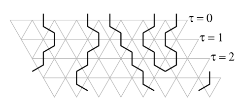
Figure 1: On this diagram of a cylindrical system, there are four strings; one of them doubles back between times $2$ and $3$. In the fermionic picture, there are five fermions at time $0$. The doubling back is interpreted as annihilation of a pair of fermions.

This paper is concerned solely with zero-temperature TIAFM systems on cylinders of finite circumference. Section 2 of Part 1 showed how to represent bond configurations by string diagrams and, by interpreting the strings as particle worldlines, reformulated the model as one of fermions hopping on a ring and evolving in imaginary time. The number-conserving transfer matrix, obtained by forbidding the zero-temperature string diagram motif , was shown to be

$${\mathbb{T}}_{0}=e^{-{H}_{0}+iP/2},$$ (1)

where

$${H}_{0}=\sum_{q\in\mathrm{BZ}}{\varepsilon}(q)n(q),\qquad P=\sum_{q\in\mathrm{BZ}}q\,n(q),$$ (2)

are a Hamiltonian and total momentum operator, respectively. $n(q)=c(q)^{\dagger}c(q)$ counts the number (0 or 1) of fermions in the mode of momentum $q$ and energy

$${\varepsilon}(q)=-\ln\left(2\cos\frac{q}{2}\right).$$ (3)

The allowed fermion modes $q$ depend on the parity of the number of particles ${\cal N}$, and are given by

$$\mathrm{BZ}=\begin{cases}\frac{2\pi}{C}{\mathbb{Z}}\cap(-\pi,\pi],&{\cal N}\,\mathrm{odd}\\ \frac{2\pi}{C}\left({\mathbb{Z}}+\frac{1}{2}\right)\cap(-\pi,\pi],&{\cal N}\,\mathrm{even}.\end{cases}$$ (4)

The motif left out of the construction of ${\mathbb{T}}_{0}$, , implements annihilation of neighboring pairs of fermions (see Fig. 1). The consequences of that will now be considered in quantitative detail, via two complementary approaches. Section 2.1 incorporates pair-annihilation into the effective Hamiltonian, which thereby becomes nonhermitian. The left- and right-eigenvectors of the transfer matrix are found, making use of factorization over $(q,-q)$ subspaces. Although this provides a complete analysis of ${\mathbb{T}}$, its interpretation in terms of the original statistical mechanical problem is not so transparent. Section 2.2 thus takes a different tack. Essentially, evaluation of the partition function of a cylindrical system is treated as a two-level process. At the outer level, we sum over times of particle annihilation events. Conditioned on those events, the partition sum is a product of shorter cylinders with number-conserving boundary conditions which can be handled as in Part 1. Section 2.3 applies the results to limiting states on infinite cylinders.

2.1 full transfer matrix

A single pair annihilation event is depicted in Fig. 1. The transfer matrix must “decide” how the configuration will evolve from time $\tau$ to time $\tau+1$. This can be viewed as a two-stage process; the first stage involves selecting pairs for annihilation, and the second, moving what particles remain. This first stage is implemented by the operator

$${\mathbb{T}}_{\mathrm{pr}}=\prod_{i\in{\mathbb{Z}}_{C}}(1+c_{i+1}c_{i}),$$ (5)

which selects neighboring pairs in all possible ways from the ring indexed by ${\mathbb{Z}}_{C}$. Note that the operators in the product commute with each other, so it is unambiguous. Since the operators $\left\{c_{i+1}c_{i}\middle|i\in{\mathbb{Z}}_{C}\right\}$ square to zero, $1+c_{i+1}c_{i}=\exp(c_{i+1}c_{i})$, and since they commute with each other ${\mathbb{T}}_{\mathrm{pr}}=\prod_{i\in{\mathbb{Z}}_{C}}e^{c_{i+1}c_{i}}$. Applying commutativity again produces ${\mathbb{T}}_{\mathrm{pr}}=e^{-H_{\mathrm{pr}}}$, where

$$H_{\mathrm{pr}}=-\sum_{i\in{\mathbb{Z}}_{C}}c_{i}c_{i+1}=\sum_{0<q\in\mathrm{BZ}}2i(\sin q)\,c(-q)c(q).$$ (6)

The exponentiated expression $e^{-H_{\mathrm{pr}}}$ can be re-expanded to

$${\mathbb{T}}_{\mathrm{pr}}=\prod_{q\in\mathrm{BZ}}[1+2i\sin q\,c(q)c(-q)],$$ (7)

a form we will use below. The complete transfer matrix is then

$${\mathbb{T}}=e^{-H_{0}}e^{-H_{\mathrm{pr}}}.$$ (8)

${\mathbb{T}}_{0}$ conserves particle number ${\cal N}$, so it can be written as ${\mathbb{T}}_{0}=\bigoplus_{{\cal N}}{\mathbb{T}}_{0,{\cal N}}$, the direct sum of transfer operators acting on ${\cal N}$-eigenspaces. In fact, since ${\mathbb{T}}_{0}$ conserves the number of particles (zero or one) in each $q$-state, it can also be factorized over the individual $q$-spaces. For ease of incorporating ${\mathbb{T}}_{\mathrm{pr}}$, however, we consider a slightly coarser factorization of the fermion Fock space ${\cal F}=\bigotimes_{0\leq q\in\mathrm{BZ}}{\cal H}(q)$, where, labelling states by the occupied modes, ${\cal H}(q)$ for $q>0$ has basis $|-q,q\rangle$, $|{\varnothing}\rangle$, $|q\rangle$ and $|-q\rangle$, while ${\cal H}(0)$ has basis $|0\rangle$, $|{\varnothing}\rangle$. Correspondingly, ${\mathbb{T}}_{0}=\bigotimes_{0\leq q\in\mathrm{BZ}}{\mathbb{T}}_{0}(q)$, with ${\mathbb{T}}_{0}(q)$ diagonal in the specified basis. The full transfer matrix ${\mathbb{T}}={\mathbb{T}}_{0}{\mathbb{T}}_{\mathrm{pr}}$ also factorizes in the same way as

$${\mathbb{T}}=\bigotimes_{0\leq q\in\mathrm{BZ}}{{\mathbb{T}}}(q).$$ (9)

Consider a generic nonzero $q$. ${{\mathbb{T}}}(q)={\mathbb{T}}_{\mathrm{e}}(q)\oplus{\mathbb{T}}_{\mathrm{o}}(q)$, where ${\mathbb{T}}_{\mathrm{o}}(q)$ (subscript ‘o’ for ‘odd’) acts on the singly-occupied subspace spanned by $|q\rangle$, $|-q\rangle$ and is simply

$${\mathbb{T}}_{\mathrm{o}}(q)=e^{-\varepsilon(q)}\left(\begin{array}[]{cc}e^{iq/2}&0\\ 0&e^{-iq/2}\end{array}\right).$$ (10)

${\mathbb{T}}_{\mathrm{e}}(q)$ acts on the even-occupancy subspace. With the abbreviation $g(q):=2\sin q$ and suppressing $q$ dependence of both $g$ and $\varepsilon$, it has matrix

$${\mathbb{T}}_{\mathrm{e}}(q) =\left(\begin{array}[]{cc}e^{-2\varepsilon}&0\\ ig&1\end{array}\right)$$ (13)

$$=e^{-2\varepsilon}\left(\begin{array}[]{c}1\\ \frac{ig}{e^{-2\varepsilon}-1}\end{array}\right)\left(\begin{array}[]{cc}1&0\end{array}\right)$$ (17)

$$\quad+\left(\begin{array}[]{cc}0\\ 1\end{array}\right)\left(\begin{array}[]{cc}\frac{-ig}{e^{-2\varepsilon}-1}&1\end{array}\right),\,\mathrm{if}\,\,q\neq\frac{2\pi}{3}.$$ (21)

The second, diagonalized, form holds for $\varepsilon(q)\neq 0$. The exceptional zero-energy single particle modes occur only for $C\in 3{\mathbb{Z}}$ in the odd-${\cal N}$ sector. In that case, we have

$${\mathbb{T}}_{\mathrm{e}}\left(\frac{2\pi}{3}\right)=\left(\begin{array}[]{cc}1&0\\ i\sqrt{3}&1\end{array}\right).$$ (22)

Putting those exceptional cases aside, ${\mathbb{T}}$ has diagonalization

$${\mathbb{T}}=\sum\lambda_{i}|e_{i}\rangle\langle\theta^{i}|,\quad\langle\theta^{i}|e_{j}\rangle=\delta_{i}^{i}.$$ (23)

Compare this to the corresponding expansion

$${\mathbb{T}}_{0}=\sum\lambda_{i}|\varphi_{i}\rangle\langle\varphi_{i}|$$

for ${\mathbb{T}}_{0}$. An eigenvector $\varphi_{i}$ essentially amounts to just a list of occupied $k$-modes. $e_{i}$ is obtained from $\varphi_{i}$ by adding terms with one or more $(q,-q)$ pairs removed, while $\theta_{i}$ is obtained by adding terms with one or more $(q,-q)$ pairs added. So, $\langle\varphi_{i}|\theta^{i}\rangle=\langle\varphi_{i}|e_{i}\rangle=1$. We refer to $\varphi_{i}$ as the parent state of $e_{i}$ and $\theta^{i}$. Note that ${\mathbb{T}}$ has the same eigenvalues as ${\mathbb{T}}_{0}$. Also, $\langle{a}|{e_{i}}\rangle=0$ unless ${\cal N}(a)\leq{\cal N}(\varphi_{i})$. Similarly, $\langle{\theta^{i}}|{a}\rangle=0$ unless ${\cal N}(a)\geq{\cal N}(\varphi_{i})$.

2.2 ${\mathbb{A}}$-expansion

The diagonalized form (23) of the transfer matrix is powerful. The partition function of a length-$L$ cylinder with fixed-configuration boundary condition $a$ at the top end and $b$ at the bottom, drawn from the ring-configuration space ${\cal X}$, is

$$Z_{L}(b|a)=\langle{b}|{{\mathbb{T}}^{L}a}\rangle=\sum\lambda_{i}^{L}\langle{b}|{e_{i}}\rangle\langle{\theta^{i}}|{a}\rangle.$$ (24)

Nevertheless, an alternative method of handling ${\mathbb{T}}_{\mathrm{pr}}$, which is arguably more probabilistic in spirit, provides a useful complement. To develop it, decompose ${\mathbb{T}}_{\mathrm{pr}}$ as

$${\mathbb{T}}_{\mathrm{pr}}=\mathrm{Id}+\sum_{n=1}^{\lfloor{C/2}\rfloor}{\mathbb{A}}_{n},$$ (25)

where

$${\mathbb{A}}_{n}=\sum_{i_{k}+1<i_{k+1}:1\leq k\leq n}(c_{i_{1}}c_{{i_{1}}+1})\cdots(c_{i_{n}}c_{{i_{n}}+1})$$ (26)

simply removes $n$ nearest-neighbor particle pairs in all possible ways. Then,

$${\mathbb{T}}^{\tau}=\sideset{}{{}^{\prime}}{\sum}_{\underline{\tau},\underline{n}}{\mathbb{T}}_{0}^{\tau_{k}}{\mathbb{A}}_{n_{k}}\cdots{\mathbb{T}}_{0}^{\tau_{1}}{\mathbb{A}}_{n_{1}}{\mathbb{T}}_{0}^{\tau_{0}}.$$ (27)

The sum here is over all values of $k\geq 0$, $\tau_{0},\ldots,\tau_{k}$ and $n_{1},\ldots,n_{k}$, and the prime on the sum indicates the constraint $\tau_{0}+\cdots+\tau_{k}=\tau$. This expansion is eminently manageable because there can be at most $\lfloor C/2\rfloor$ ${\mathbb{A}}$’s inserted. For the partition function (24), we now obtain

$$Z_{L}(b|a) =\sideset{}{{}^{\prime}}{\sum}_{\underline{x},\underline{y},\underline{n},\underline{L}}Z^{0}_{L_{k}}(b|a_{k})\langle{a_{k}}|{{\mathbb{A}}_{n_{k}}b_{k}}\rangle\cdots$$

$$\qquad\langle{a_{2}}|{{\mathbb{A}}_{n_{2}}b_{2}}\rangle Z^{0}_{L_{1}}(b_{2}|a_{1})\langle a_{1}|{\mathbb{A}}_{n_{1}}b_{1}\rangle Z^{0}_{L_{0}}(b_{1}|a),$$

with $Z_{L}^{0}$ the number-conserving partition function constructed from ${\mathbb{T}}_{0}$. Note that, with the intermediate states $a_{i}$, $b_{i}$ being delta functions on single configurations in ${\cal X}$, the factors $\langle a_{m}|{\mathbb{A}}_{n_{m}}b_{m}\rangle$ are either zero or one. Effective use of the expansion (27) for large $L$ hinges on the fact that ${\mathbb{T}}_{0}$ is transitive on each fixed-particle-number configuration space ${\cal X}_{N}\subset{\cal X}$. For then, according to the Perron-Frobenius theorem, the leading eigenvalue of the restriction ${\mathbb{T}}_{0}|_{{\cal X}_{N}}$ is nondegenerate and has strictly positive weight on each configuration in ${\cal X}_{N}$. Thus, if $N={\cal N}(a)={\cal N}(b)$, then for large $L$,

$$Z_{L}^{0}(b|a)\sim\langle b|\varphi_{N,0}\rangle\lambda_{N,0}^{L}\langle\varphi_{N,0}|a\rangle,$$

where $\lambda_{N,0}$ is the largest eigenvalue of ${\mathbb{T}}_{0}|_{{\cal X}_{N}}$ and $\varphi_{N,0}$ is the corresponding eigenvector. More generally

$$Z_{L}(b|a)\sim c\Big{(}\mathrm{max}\,\{\lambda_{N^{*},0}\,;\,{\cal N}(b)\leq N^{*}\leq{\cal N}(a)\}\Big{)}^{L}.$$ (28)

Using the expansion (27), the argument for this is that the sum is dominated by configurations where the ${\mathbb{A}}$’s are clustered at either end so as to allow most of the length of the cylinder to have $N^{*}$ particles, where $N^{*}$ is the maximizing value in (28). The only exception to this is if the maximizing $N^{*}$ is not unique. This occurs only in the odd-${\cal N}$ sector with $C\in 3{\mathbb{N}}$. In that case, if ${\cal N}(b)\leq 2C/3-1$ and ${\cal N}(a)\geq 2C/3+1$, there will be a transition between the two particle numbers effected by destroying two particles in the zero-energy mode, and it will occurs indifferently anywhere along the length of the cylinder. The result in that case is $Z_{L}(b|a)\sim cL\lambda_{2C/3-1,0}^{L}$.

The ${\mathbb{A}}$-expansion can be leveraged to draw conclusions about the eigenfunctions of the full transfer matrix ${\mathbb{T}}$. An important example is that,

$$\langle b|e_{0}\rangle \neq 0\;\,\mathrm{iff}\;\,{\cal N}(b)\leq{\cal N}^{p}_{c}(C),\qquad$$

$$\langle\theta^{0}|b\rangle \neq 0\,\;\mathrm{iff}\;\,{\cal N}_{c}^{p}(C)\leq{\cal N}(b),$$ (29)

where

$${\cal N}_{c}^{\mathrm{even}}(C)=2\left\lfloor\frac{C}{3}+\frac{1}{2}\right\rfloor,\quad{\cal N}_{c}^{\mathrm{odd}}(C)=2\left\lfloor\frac{C}{3}\right\rfloor+{1}$$ (30)

are the numbers of single-particle modes of non-negative energy in the even-${\cal N}$ and odd-${\cal N}$ sectors, respectively. We give the argument for $\langle b|e_{0}\rangle$. The implication from left to right has been established above. So, take $a$ such that ${\cal N}(a)={\cal N}_{c}^{p}(C)$. It is clear from the Perron-Frobenius theorem that both $\langle a|e_{0}\rangle$ and $\langle\theta^{0}|a\rangle$ are nonzero since ${\mathbb{T}}_{0}$ is transitive on ${\cal X}_{{\cal N}{a}}$. From the ${\mathbb{A}}$-expansion, if ${\cal N}(b)\leq{\cal N}^{p}_{c}(C)$, we know that $Z_{L}(b|a)\sim c\lambda_{0}^{L}$. But, from (24), this is impossible unless $\langle b|e_{0}\rangle\neq 0$. The argument for the other equivalence is analogous.

In a similar vein, writing

$$\overline{1}:=\sum_{a\in{\cal X}}a$$ (31)

for the state uniformly distributed over all configurations (this corresponds to open boundary conditions), both $\langle{\overline{1}}|{e_{0}}\rangle$ and $\langle{\theta^{0}}|{\overline{1}}\rangle$ are nonzero. To see the first of these, choose configurations $a,b$ such that $\langle{b}|{e_{0}}\rangle\langle{\theta^{0}}|{a}\rangle\neq 0$. Then, by positivity of ${\mathbb{T}}_{0}$, $Z_{L}(\overline{1}|a)\geq Z_{L}(b|a)\sim\lambda_{0}^{L}$, which implies that $\langle{\overline{1}}|{e_{0}}\rangle\neq 0$. An extension of the same reasoning leads to a conclusion which will be useful in Section 4.2. Namely, suppose that the first excited state, $\varphi_{1}$, has two more particles than does $\varphi_{0}$. Then, for any configuration with ${\cal N}(b)={\cal N}(\varphi_{1})$, $\langle{b}|{e_{0}}\rangle=0$, $\langle{b}|{e_{1}}\rangle\neq 0$. So, there are configurations $a$ with $Z_{L}(b|a)\sim\lambda_{1}^{L}$. As before, by positivity of ${\mathbb{T}}$, we conclude that $\langle{\theta^{1}}|{\overline{1}}\rangle\neq 0$. Note that this does not prove that $\langle{\overline{1}}|{e_{1}}\rangle\neq 0$.

2.3 Ground macrostates on an infinite cylinder

Now we examine the structure of ground macrostates on an infinite cylinder. These are limits of sequences of states for a cylinder with fixed $C$ and $-L_{1}\leq\tau\leq L_{2}$ as $L_{1},L_{2}\to\infty$, possibly at different rates. From the earlier discussion of the ${\mathbb{A}}$-expansion around (28), we know that with fixed configurations $b$ and $a$ as boundary conditions, the bulk settles into the state $\varphi_{N^{*},0}$, where $N^{*}$ with ${\cal N}(b)\leq N^{*}\leq{\cal N}(a)$ is the unique maximizer of $\lambda_{N^{*},0}$, at least if there are no zero-energy modes. Thus, the probability of the ring configurations $X_{t}$ and $X_{s}$ at imaginary times $t$ and $s$ ($\geq t$) being $x$ and $y$, respectively, is

$$\langle\delta_{x}(X_{t})\delta_{y}(X_{s})\rangle=\langle\varphi_{N^{*},0}|y\rangle\frac{Z_{s-t}^{0}(y|x)}{\lambda_{N,0}^{s-t}}\langle{x}|{\varphi_{N^{*},0}}\rangle.$$

$Z^{0}$ can be used here rather than $Z$ since there is no change of ${\cal N}$. The connected correlation function

$$\langle\delta_{x}(X_{t});\delta_{y}(X_{s})\rangle_{\cal N}:= \langle\delta_{x}(X_{t})\delta_{y}(X_{s})\rangle_{\cal N}$$

$$-\langle\delta_{x}(X_{t})\rangle_{\cal N}\langle\delta_{y}(X_{s})\rangle_{\cal N},$$ (32)

is thus

$$\langle\delta_{x}(X_{t}) ;\delta_{y}(X_{s})\rangle_{\cal N}=$$ (33)

$$\sum_{i>0}\left(\frac{\lambda_{{\cal N},i}}{\lambda_{{\cal N},0}}\right)^{s-t}\langle{\varphi_{{\cal N},0}}|{y}\rangle\langle{y}|{\varphi_{{\cal N},i}}\rangle\langle{\varphi_{{\cal N},i}}|{x}\rangle\langle{x}|{\varphi_{{\cal N},0}}\rangle.$$

Generically, for functions $f,g:{\cal X}\rightarrow{\mathbb{R}}$,

$$\langle f(X_{t})\,;\,g(X_{s})\rangle_{\cal N}\sim c\left|\frac{\lambda_{{\cal N},1}}{\lambda_{{\cal N},0}}\right|^{s-t}.$$ (34)

For odd ${\cal N}$ and $C\in 3{\mathbb{Z}}$ zero-energy modes complicate matters slightly. The interesting boundary configurations have ${\cal N}(a)$ big enough to include the zero-energy modes and ${\cal N}(b)$ small enough to exclude them. Then, the total entropy of the entire system is insensitive to the location of the transition (or “domain wall”), and the distribution of its location is uniform over the entire length of the cylinder. With $s$ and $t$ as above fixed and finite, the probability that domain wall occurs between them goes to zero. The state in the bulk thus converges to a probabilistic mixture of $\varphi_{{\cal N},0}$ and $\varphi_{{\cal N}+2,0}$, where the former excludes the zero-energy modes and the latter includes them. The probability that $s$ and $t$ are on one side or the other of the domain wall is determined by the relative rates of divergence of $L_{1}$ and $L_{2}$. The limiting state is the same as that obtained by a mixture of number-conserving boundary conditions. Thus, in the infinite-length limit, the Perron-Frobenius scenario is effectively restored, as far as the bulk is concerned. Every infinite-cylinder state is a probabilistic mixture of the extremal states (pure phases) which have well-defined values of ${\cal N}$. Decay of connected correlation functions, as in Eq. (34), has the same relation to eigenvalues of the transfer matrix as for thermally disordered systems.

3 ring-to-ring mutual information on infinite cylinders

Traditional one- and two-spin correlation functions, e.g., $\langle\sigma_{i}\rangle$ and $\langle\sigma_{i}\sigma_{j}\rangle$, tell us everything there is to know about the distribution of one spin conditioned on the value of another, not only how much the conditional distribution differs from the marginal, but also in what way (is the correlation ferromagnetic or antiferromagnetic?). For more complex random variables, e.g. bond values on a ring around the cylinder, it is not clear how to describe in what way they are dependent, but a simple measure of the strength of dependence is available in the form of mutual information. We recall Shannon and Weaver (1949); Billingsley (1965); Csiszár and Körner (1981); Cover and Thomas (1991) that the entropy of a discrete random variable $Y$ is given by

$$H(Y)=-\sum_{y}P_{Y}(y)\ln P_{Y}(y).$$ (35)

The conditional entropy given a second random variable $X$ by

$$H(Y|X)=-\sum_{x}P_{X}(x)\sum_{y}P_{Y}(y|X=x)\ln P_{Y}(y|X=x),$$ (36)

and the mutual information between the two by

$$I(X\!:\!Y) =\sum_{x,y}P_{XY}(x,y)\ln\frac{P_{XY}(x,y)}{P_{X}(x)P_{Y}(y)}$$

$$=H(X)+H(Y)-H(X,Y)$$

$$=H(Y)-H(Y|X).$$ (37)

The last form here obscures that $I(X\!:\!Y)=I(Y\!:\!X)$, but expresses clearly that $I(X\!:\!Y)$ measures the average amount of information $X$ carries about $Y$ insofar as it is the amount by which the uncertainty about $Y$ is reduced by the knowledge of the value of $X$. Calculations below will mostly work from the first expression in (3).

3.1 ring-to-ring mutual information on infinite cylinders

As shown in Section 2.3, a zero-temperature pure phase of an infinite cylinder (ring indices in ${\mathbb{Z}}$) is labelled by a definite particle number ${\cal N}$, and in such a state the joint probability of configurations $X_{0}$ and $X_{\tau}$ on rings $0$ and $\tau$, respectively, is

$${\kern-10.00002pt}P_{\cal N}(X_{0}=a\,\&\,X_{\tau}=b)=\langle\varphi_{{\cal N},0}|b\rangle\frac{Z_{\tau}(b|a)}{\lambda_{{\cal N},0}^{\tau}}\langle a|\varphi_{{\cal N},0}\rangle.$$ (38)

Since only the ${\cal N}$-particle configuration subspace ${\cal X}_{\cal N}$ will be relevant in this subsection, ‘${\cal N}$’ subscripts will be dropped until further notice, in order to simplify expressions. The probabilities in (38) provide the building blocks for the mutual information between $X_{0}$ and $X_{\tau}$, which thus has expression (${\cal N}$ now implicit)

$$I_{\infty}(X_{0}\!:\!X_{\tau})=\sum_{a,b\in{\cal X}_{\cal N}}\langle\varphi_{0}|b\rangle\langle a|\varphi_{0}\rangle\frac{Z_{\tau}(b|a)}{\lambda_{0}^{\tau}}\ln\frac{\lambda_{0}^{-\tau}Z_{\tau}(b|a)}{\langle\varphi_{0}|a\rangle\langle b|\varphi_{0}\rangle}.$$ (39)

Asymptotically in $\tau$, both $\lambda_{0}^{-\tau}{Z_{\tau}(b|a)}$ and the argument of the logarithm in (39) tend to one. Thus, the leading contribution to the mutual information comes from the logarithm. Precisely, recalling that the restricted transfer matrix is diagonalized by states labelled with ${\cal N}$ $k$-vectors, (39) can be rewritten as

$$I_{\infty}(X_{0}\!:\!X_{\tau})=\sum_{a,b,j} \langle a|\varphi_{0}\rangle\langle\varphi_{0}|b\rangle\langle{b}|{\varphi_{j}}\rangle\langle{\varphi_{j}}|{a}\rangle\times$$

$$\quad\left(\frac{\lambda_{j}}{\lambda_{0}}\right)^{\tau}\ln W_{\tau}(b|a),$$ (40)

where

$$W_{\tau}(b|a){\kern 1.99997pt}:{\kern-5.0pt}={\kern 1.99997pt}1+\sum_{i>0}\left(\frac{\lambda_{i}}{\lambda_{0}}\right)^{\tau}\frac{\langle{b}|{\varphi_{i}}\rangle\langle{\varphi_{i}}|{a}\rangle}{\langle{b}|{\varphi_{0}}\rangle\langle{\varphi_{0}}|{a}\rangle}.$$ (41)

At first glance, it would appear that the asymptotic behavior of $I_{\infty}(X_{0}\!:\!X_{\tau})$ is found by taking $j=0$ and replacing $\ln W_{\tau}(b|a)$ by the $i=1$ term in the sum. This is wrong for two reasons: some surprising cancellations take place, and there are two distinct eigenvalues with second largest modulus. The fermion ground state is a filled Fermi sea, and the lowest energy excitations are particle-hole pairs. There are two such, and they are converted one into the other by reversing all momenta. Correspondingly, $\overline{\lambda_{1}}=\lambda_{2}$. Expanding $\ln W_{\tau}(b|a)$ in powers of the sum, and using that $\langle{b}|{\varphi_{0}}\rangle$ is real, the first-order term (in the logarithmic expansion) is

$$\sum_{j}\sum_{i>0}\left(\frac{\lambda_{j}\lambda_{i}}{\lambda_{0}^{2}}\right)^{\tau}\sum_{a,b}\langle{b}|{\varphi_{j}}\rangle\langle{\varphi_{j}}|{a}\rangle{\langle{b}|{\varphi_{i}}\rangle\langle{\varphi_{i}}|{a}\rangle}.$$

Since $\left\{\Psi(X)\middle|X\in{\cal X}_{\cal N}\right\}$ comprises an orthonormal basis for the ${\cal N}$-particle Hilbert space, when $j=0$, the sums over $a$ and $b$ produce factors $\langle{\varphi_{0}}|{\varphi_{i}}\rangle$. Checking the nominally next-largest terms, $i=j=1$ and $i=j=2$ are also seen to give vanishing contributions since, for example, $\langle{b}|{\varphi_{1}}\rangle\langle{b}|{\varphi_{1}}\rangle=\langle{\varphi_{2}}|{b}\rangle\langle{b}|{\varphi_{1}}\rangle$, which, summed over $b$ yields zero. Finally, though, $j=1$, $i=2$ and $j=2$, $i=1$ give nonvanishing contributions. The result is $2|\lambda_{1}/\lambda_{0}|^{2\tau}$. However, we are not done, since the second-order term in the expansion of the logarithm competes with this, when $j=0$. Evaluating this using the same observations as in the preceding calculations, we find a contribution $-|\lambda_{1}/\lambda_{0}|^{2\tau}$. All together, up to relatively exponentially small corrections, and restoring the ‘${\cal N}$’ indices, we find

$$I_{\infty,{\cal N}}(X_{0}\!:\!X_{\tau})\sim\left|\frac{\lambda_{{\cal N},1}}{\lambda_{{\cal N},0}}\right|^{2\tau}.$$ (42)

A remarkable feature of this result is that the coefficient is exactly one. In fact, it depends only on some simple spectral properties of the transfer matrix, as a review of our computations reveals. For a real transfer matrix with a nondegenerate eigenvalue of largest modulus (e.g., Perron-Frobenius scenario) and all generalized eigenspaces of subleading eigenvalue modulus having equal geometric and algebraic degeneracy, the mutual information is asymptotically as in (42), with a prefactor equal to half the total dimension of all eigenspaces of subleading modulus. Comparing to (34), we see that $I_{\infty,{\cal N}}(X_{0}\!:\!X_{\tau})$ decays at a rate twice that of connected correlations of the form $\langle f(X_{0})\,;\,g(X_{\tau})\rangle_{{\cal N}}$.

3.2 explanation of the exponent

In the Perron-Frobenius scenario, generic truncated correlation functions fall off as

$$\langle f(X_{u})g(X_{u+s})\rangle-\langle f(X_{u})\rangle\langle g(X_{u+s})\rangle\sim c\left|\frac{\lambda_{{\cal N},1}}{\lambda_{{\cal N},0}}\right|^{s},$$ (43)

asymptotically as the separation $s$ along the cylinder tends to infinity. As just demonstrated, $I_{\infty,{\cal N}}(X_{0}\!:\!X_{\tau})$ falls off at twice the rate of an ordinary correlation function. This may seem inconsistent, but one must remember that the mutual information is not an ordinary correlation function.

An explanation will now be given of why $I_{\infty,{\cal N}}(X_{0}\!:\!X_{\tau})$ has the decay rate it does. It is really just a matter of the character of mutual information. Thus, we consider now an arbitrary pair of discrete random variables $X$ and $Y$, not necessarily connected to the TIAFM at all, thereby also reducing notational clutter. Denote possible values of $X$ and $Y$ by greek ($\alpha$,…) and latin ($i$,…) letters, respectively, so that we can write simply $P(i|\alpha)$ instead of $P(Y=i|X=\alpha)$, etc. Abbreviate

$$\delta_{\alpha}P(i)=P(i|\alpha)-P(i),$$ (44)

the idea being that $X$ and $Y$ are very nearly independent, so that $\delta_{\alpha}P(i)$ is small. We shall expand in its powers of these. First, however, note that

$$P(\alpha)\delta_{\alpha}P(i)=P(i,\alpha)-P(i)P(\alpha)$$ (45)

is just an ordinary truncated correlation function.

Using the new notation, the mutual information between $X$ and $Y$ is

$$I(X\!:\!Y)= \sum_{\alpha}P(\alpha)\sum_{i}\Big{\{}[P(i)+\delta_{\alpha}P(i)]\ln[P(i)+\delta_{\alpha}P(i)]$$

$$-P(i)\ln P(i)\Big{\}}$$

Expand in powers of the $\delta_{\cdot}P(\cdot)$’s to obtain

$$I(X\!:\!Y)= \sum_{\alpha,i}[1+\ln P(i)]P(\alpha)\delta_{\alpha}P(i)$$

$$+\frac{1}{2}\sum_{\alpha,i}P(\alpha)\frac{[\delta_{\alpha}P(i)]^{2}}{P(i)}+\cdots$$

Outside the square brackets in the first sum is the truncated correlation function (45). Thus, the sum over $\alpha$ will vanish, leaving just.

$$I(X\!:\!Y)\sim\sum_{\alpha,i}\frac{[P(\alpha)\delta_{\alpha}P(i)]^{2}}{P(\alpha)P(i)}.$$

Again, the truncated correlation function appears, now squared. Now interpret in the context where $X$ and $Y$ are $X_{u}$ and $X_{u+s}$ to conclude that $I_{\infty,{\cal N}}(X_{0}\!:\!X_{\tau})$ falls off at twice the rate of an ordinary correlation function.

Note that expansion in powers of $\delta_{\alpha}P(i)$ will be thwarted if the event $Y=i$ requires $X=\alpha$. This is the situation faced for the end-to-end MI of the zero-temperature cylindrical TIAFM.

4 end-to-end mutual information on finite-length cylinders

4.1 energy gaps

As just noted, the correlation length in the ${\cal N}$ phase is twice the decay length of the ring-to-ring mutual information. In terms of the fermion picture, the correlation length is the reciprocal of $\Delta\varepsilon=\ln|\lambda_{{\cal N},0}/\lambda_{{\cal N},1}|$, the fundamental energy gap of the ${\cal N}$-particle subspace. This section takes a detailed look at the unrestricted fundamental energy gaps, since those are the relevant ones for the decay of end-to-end mutual information under open boundary conditions.

Recall that according to (4), allowed single-particle momenta satisfy

$$\frac{q}{\delta}\in\begin{cases}{\mathbb{Z}},&{\cal N}\,\mathrm{odd},\\ {\mathbb{Z}}+\frac{1}{2},&{\cal N}\,\mathrm{even},\end{cases}$$ (46)

where $\delta=2\pi/C$ is the finesse of the momentum spectrum. For an infinite cylinder, the even/odd distinction between these cases is not so important. $\varphi_{{\cal N},0}$ corresponds to a filled Fermi sea with $n$ particles, and $\varphi_{{\cal N},1}$ is a particle-hole excitation with a particle in the highest occupied mode of $\varphi_{{\cal N},0}$ promoted to the lowest unoccupied mode. For large $C$ this gap is $\Delta\varepsilon\simeq v(q_{F})\delta=2\pi v(q_{F})/C$, where the band velocity

$$v(q)=\frac{1}{2}\tan\frac{q}{2}$$

was derived in Section 2 of Part 1.

When unrestricted gaps are considered, the situation is more intricate and the distinction between even-${\cal N}$ and odd-${\cal N}$ sectors matters, since not only differences between energies of single-particle modes are relevant, but also their exact values. Recall that, in the absence of zero-energy modes, eigenstates of ${\mathbb{T}}$ are descended from those of ${\mathbb{T}}_{0}$, with the same eigenvalues. Thus, it suffices here to analyze the parent states. The ground state has all modes with $|q|<q_{0}=2\pi/3=(C/3)\delta$ occupied. Writing $C=3p+m$, with $p,m\in{\mathbb{N}}$, we get $q_{0}/\delta=p+m/3$. We now use a linearization of the dispersion relation around $q_{0}$ to determine the fundamental gaps. Only a couple of cases will require attention to the curvature. Then, the energy cost of a particle-hole excitation is always $v(q_{0})\delta\simeq\sqrt{3}\pi/C$, as noted in the previous paragraph. But we will see that, over ${\cal X}$, these are never the lowest-energy excitations.

Now specialize to odd ${\cal N}$. According to Eq. (46), allowed momenta are integers. If $C\equiv 1$ (mod 3), then removing the particles from modes $q=\pm(q_{0}-\delta/3)$ has an energy cost of only $(2/3)v(q_{0})\delta$. Clearly, this is the lowest-energy excitation. The conclusion is reported as an entry in Table 1. In case $C\equiv 2$ (mod 3), the lowest energy excitation is obtained by adding particles to $\pm(q_{0}+\delta/3)$, with the same cost. The case $m=0$ is very different, and different from anything in the even ${\cal N}$ sector, for this is the case with zero-energy modes. The two degenerate states of ${\mathbb{T}}_{0}$, one with all levels filled up to and including the zero-energy modes, and the other with the zero-energy modes empty, descend to the two-dimensional generalized ground eigenspace of ${\mathbb{T}}$. As far as ${\mathbb{T}}_{0}$ is concerned, the gap is zero.

Turn now to the even ${\cal N}$ sector. If $C\equiv 1$ (mod 3), the the lowest excitation adds particles to $\pm(q_{0}+\delta/6)$, and if $L\equiv 2$ (mod 3), removes particles from $\pm(q_{0}-\delta/6)$. In either case, the cost is $(1/3)v(q_{0})\delta$. In case $L\equiv 0$ (mod 3), the pp, hh, and ph excitations are all degenerate in the linearized approximation, with energy $v(q_{0})\delta$. However, since $\varepsilon(q)$ is convex, the hh excitation will be slightly lower in energy.

Apart from $L\equiv 0$ (mod 3) with even ${\cal N}$, there is one other specific cylinder with $C\geq 3$ for which the linearized approximation leads to an incorrect conclusion. That is $C=5$ for odd ${\cal N}$. In this case, the hh excitation is actually exactly degenerate with the pp excitation, as a straightforward computation shows.

${\cal N}$ parity	even			odd
$C$ mod 3	0	1	2	0	1	2
excitation type	hh	pp	hh	hh	hh	pp
$\Delta\varepsilon\cdot C/(\pi\sqrt{3})$	1	1/3	1/3	0	2/3	2/3

Table 1: fundamental energy gaps $\Delta\varepsilon$ of ${\mathbb{T}}_{0}$ and corresponding excitation types. ‘hh’ and ‘pp’ indicate excitations involving removal (addition) of two particles. Energies are reported in units of $v(q_{0})\delta=(\sqrt{3}/2)(2\pi/C)=\pi\sqrt{3}/C$, according to a linearized approximation of $\varepsilon(q)$. Due to the strict convexity of $\varepsilon(q)$, energies reported for hh (pp) excitations are overestimates (underestimates), though the relative error goes to zero as $C\to\infty$.

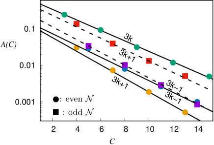
Figure 2: Amplitudes $A(L)$ [see (57)] of the asymptotic decay of end-to-end mutual information Nourhani et al. (2018).

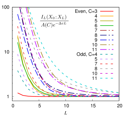
Figure 3: Ratio of the end-to-end mutual information $I_{L}(X_{0}\!:\!X_{L})$ to the leading behavior $A(C)e^{-\Delta\varepsilon L}$, for cases without zero-energy modes and $3\leq C\leq 11$. The approach is always from above because the leading behavior correctly accounts for all information transmission via the first two eigenmodes, but not the others Nourhani et al. (2018).

4.2 open boundary end-to-end mutual information without zero-energy modes

In this subsection, we compute the asymptotic behavior of the end-to-end mutual information for a cylinder with open boundary conditions in cases without zero-energy modes; the exceptional case $C\equiv 0$ (mod 3), ${\cal N}$ odd, will be treated in Section 4.4. The reader wishing to skip the intricacies of the calculations should go to the results in (56), (57), and (58).

Mutual information is a property of a joint probability distribution. In an equilibrium statistical mechanics context, probabilities come from partition functions, which for the problem at hand just count ground microstates. As before, $Z_{L}(b|a)$ here denotes the partition function with configurations $X_{0}$ and $X_{L}$ on the end rings of a length-$L$ cylinder fixed to $a$ and $b$, respectively, and $Z_{L}(\overline{1}|\overline{1})$ is the open boundary condition partition function. The mutual information between the configurations $X_{0}$ and $X_{L}$ at the ends of a length-$L$ cylinder is then

$$I_{L}(X_{0}\!:\!X_{L})=\sum_{(a,b)\in{\cal X}^{2}}\frac{Z_{L}(b|a)}{Z_{L}(\overline{1}|\overline{1})}\ln\frac{Z_{L}(b|a)Z_{L}(\overline{1}|\overline{1})}{Z_{L}(b|\overline{1})Z_{L}(\overline{1}|a)}.$$ (47)

$Z_{L}(b|a)$ can be written in terms of the ring-to-ring transfer matrix ${\mathbb{T}}$. In the absence of zero-energy modes, ${\mathbb{T}}=\sum_{i}\lambda_{i}|e_{i}\rangle\langle\theta^{i}|$ has eigenvalues $\lambda_{0}>|\lambda_{1}|\geq|\lambda_{2}|\cdots$. So,

$$Z_{L}(b|a)=\langle b|{\mathbb{T}}^{L}a\rangle=\sum\lambda_{i}^{L}\langle b|e_{i}\rangle\langle\theta^{i}|a\rangle.$$ (48)

To be able to extract the asymptotic behavior of $I_{L}(X_{0}\!:\!X_{L})$, we need to classify boundary configurations according to the largest-modulus eigenvalue state with which they have nonzero overlap. Accordingly, we introduce the sets of configurations (${\cal T}$ for ‘top’ and ${\cal B}$ for ‘bottom’, i.e., of the cylinder)

$${\cal B}_{0} {\kern 1.99997pt}:{\kern-5.0pt}={\kern 1.99997pt}\left\{b\in{\cal X}\middle|\langle{b}|{\theta^{0}}\rangle\neq 0\right\},$$

$${\cal B}_{1} {\kern 1.99997pt}:{\kern-5.0pt}={\kern 1.99997pt}\left\{b\in{\cal X}\middle|\langle{b}|{\theta^{0}}\rangle=0,\langle{b}|{\theta^{1}}\rangle\neq 0\right\},$$

$${\cal T}_{0} {\kern 1.99997pt}:{\kern-5.0pt}={\kern 1.99997pt}\left\{a\in{\cal X}\middle|\langle{e_{0}}|{a}\rangle\neq 0\right\},$$

$${\cal T}_{1} {\kern 1.99997pt}:{\kern-5.0pt}={\kern 1.99997pt}\left\{a\in{\cal X}\middle|\langle{e_{0}}|{a}\rangle=0,\langle{e_{1}}|{a}\rangle\neq 0\right\}.$$ (49)

Various facts about the overlaps found near the end of Section 2.2 will be called upon in the following.

4.2.1 $(b,a)\in{\cal B}_{0}\times{\cal T}_{0}$

If the contribution of these configurations does not vanish, then they dominate the asymptotic behavior of $I_{L}(X_{0}\!:\!X_{L})$. We shall see, however, that this contribution does vanish. For these boundary configuration pairs, write

$$Z_{L}(b|a)=\lambda_{0}^{L}\langle b|e_{0}\rangle\langle\theta^{0}|a\rangle W_{L}(b|a),$$ (50)

with

$$W_{L}(b|a){\kern 1.99997pt}:{\kern-5.0pt}={\kern 1.99997pt}1+\sum_{i>0}\left(\frac{\lambda_{i}}{\lambda_{0}}\right)^{L}\frac{\langle{b}|{e_{i}}\rangle\langle{\theta^{i}}|{a}\rangle}{\langle{b}|{e_{0}}\rangle\langle{\theta^{0}}|{a}\rangle}.$$ (51)

The contribution of ${\cal B}_{0}\times{\cal T}_{0}$ end configurations to the mutual information is

$$I_{L}^{{\cal B}_{0}\times{\cal T}_{0}}(X_{0}\!:\!X_{L})=\sum_{{\cal B}_{0}\times{\cal T}_{0}}\Big{\{} \frac{\langle{b}|{e_{0}}\rangle\langle{\theta^{0}}|{a}\rangle}{\langle{\overline{1}}|{e_{0}}\rangle\langle{\theta^{0}}|{\overline{1}}\rangle}\frac{W_{L}(b|a)}{W_{L}(\overline{1}\overline{1})}\times$$

$$\;\ln\frac{W_{L}(b|a)W_{L}(\overline{1}\overline{1})}{W_{L}(b\overline{1})W_{L}(\overline{1}a)}\Big{\}}.$$ (52)

Asympototically as $L\to\infty$,

$$\ln W_{L}(b|a)\sim\left(\frac{\lambda_{1}}{\lambda_{0}}\right)^{L}\frac{\langle{b}|{e_{1}}\rangle\langle{\theta^{1}}|{a}\rangle}{\langle{b}|{e_{0}}\rangle\langle{\theta^{0}}|{a}\rangle}.$$ (53)

In writing this, we rely on the conclusion of the previous subsection (Table 1), that for $C\geq 3$ (with one exception: $C=5$, odd ${\cal N}$), there is a single nondegenerate eigenvalue of subleading modulus, $\lambda_{1}$, which is real. Remarks on the exceptional case will be made momentarily. Therefore,

$$I_{L}^{{\cal B}_{0}\times{\cal T}_{0}}(X_{0}\!:\!X_{L})\sim\left(\frac{\lambda_{1}}{\lambda_{0}}\right)^{L}\frac{1}{\langle{\overline{1}}|{e_{0}}\rangle\langle{\theta^{0}}|{\overline{1}}\rangle}\sum_{b\in{\cal B}_{0},a\in{\cal T}_{0}}\Bigg{[} \langle{b}|{e_{1}}\rangle\langle{\overline{1}}|{a}\rangle+\langle{b}|{e_{0}}\rangle\langle{\theta^{0}}|{a}\rangle\frac{\langle{\overline{1}}|{e_{1}}\rangle\langle{\theta^{1}}|{\overline{1}}\rangle}{\langle{\overline{1}}|{e_{0}}\rangle\langle{\theta^{0}}|{\overline{1}}\rangle}$$

$$-\langle{b}|{e_{1}}\rangle\langle{\theta^{0}}|{a}\rangle\frac{\langle{\theta^{1}}|{\overline{1}}\rangle}{\langle{\theta^{0}}|{\overline{1}}\rangle}-\langle{b}|{e_{0}}\rangle\langle{\theta^{1}}|{a}\rangle\frac{\langle{\overline{1}}|{e_{1}}\rangle}{\langle{\overline{1}}|{e_{0}}\rangle}\Bigg{]}.$$ (54)

The sum here actually vanishes. To see that, consider the two cases ${\cal N}(\varphi_{1})={\cal N}(\varphi_{0})-2$, or ${\cal N}(\varphi_{1})={\cal N}(\varphi_{0})+2$. In the first case, $\langle{b}|{e_{1}}\rangle\neq 0$ implies that ${\cal N}(b)\leq{\cal N}(\varphi_{1})={\cal N}(\varphi)-2$. But, then, $\langle{b}|{e_{0}}\rangle\neq 0$, and the sum over $b$ can be expanded to all of ${\cal X}$ since the added terms give zero anyway. The resulting sums over $b$ of the first term in square brackets cancels that of the final term, and similarly the second and third terms. In the other case, ${\cal N}(\varphi_{1})={\cal N}(\varphi_{0})+2$, proceed similarly, but expand the range of $a$ instead. In the exceptional case ($C=5$, odd ${\cal N}$), expression (53) would have a second term, but their separate contributions are zero, as just seen.

Thus, $I_{L}^{{\cal B}_{0}\times{\cal T}_{0}}(X_{0}\!:\!X_{L})$ is exponentially small compared to $(\lambda_{1}/\lambda_{0})^{L}$; we must turn to the contributions of other boundary configurations: $b$ in ${\cal B}_{1}$ or $a$ in ${\cal T}_{1}$. The first case requires ${\cal N}(b)\geq{\cal N}(\varphi_{1})={\cal N}(\varphi_{0})+2$, hence essentially corresponds to a pp excitation, whereas the second case requires ${\cal N}(a)\leq{\cal N}(\varphi_{1})={\cal N}(\varphi_{0})-2$, corresponding to a hh excitation. We compute their contributions separately and then add them. Since the calculations are similar, only the ${\cal B}_{1}\times{\cal T}_{0}$ need be discussed in any detail.

4.2.2 $(b,a)\in{\cal B}_{1}\times{\cal T}_{0}$

In this case,

$$\frac{Z_{L}(b|a)}{Z_{L}(\overline{1}|\overline{1})}\sim\frac{\langle{b}|{e_{1}}\rangle\langle{\theta^{1}}|{a}\rangle}{\langle{\overline{1}}|{e_{0}}\rangle\langle{\theta^{0}}|{\overline{1}}\rangle}\left(\frac{\lambda_{1}}{\lambda_{0}}\right)^{L},$$

and

$$\frac{Z_{L}(b|a)Z_{L}(\overline{1}|\overline{1})}{Z_{L}(b|\overline{1})Z_{L}(\overline{1}|a)}\sim\frac{\langle{\theta^{1}}|{a}\rangle\langle{\theta^{0}}|{\overline{1}}\rangle}{\langle{\theta^{1}}|{\overline{1}}\rangle\langle{\theta^{0}}|{a}\rangle}.$$ (55)

Inserting these into (47), we find a contribution to the end-to-end mutual information of

$$I_{L}^{{\cal B}_{1}\times{\cal T}_{0}}(X_{0}\!:\!X_{L})\sim A^{{\cal B}_{1}\times{\cal T}_{0}}(C)\left(\frac{\lambda_{1}}{\lambda_{0}}\right)^{L},$$ (56)

where

$$A^{{\cal B}_{1}\times{\cal T}_{0}}(C)= \sum_{{\cal N}(b)>{\cal N}(\varphi_{0}),\,a\in{\cal T}_{0}}\frac{\langle{b}|{e_{1}}\rangle\langle{\theta^{1}}|{a}\rangle}{\langle{\overline{1}}|{e_{0}}\rangle\langle{\theta^{0}}|{\overline{1}}\rangle}\ln\frac{\langle{\theta^{1}}|{a}\rangle\langle{\theta^{0}}|{\overline{1}}\rangle}{\langle{\theta^{1}}|{\overline{1}}\rangle\langle{\theta^{0}}|{a}\rangle}$$

$$= \sum_{{\cal N}(a)\geq{\cal N}(\varphi_{0})+2}\frac{\langle{\overline{1}}|{\varphi_{1}}\rangle\langle{\theta^{1}}|{a}\rangle}{\langle{\overline{1}}|{e_{0}}\rangle\langle{\theta^{0}}|{\overline{1}}\rangle}\ln\frac{\langle{\theta^{1}}|{a}\rangle\langle{\theta^{0}}|{\overline{1}}\rangle}{\langle{\theta^{1}}|{\overline{1}}\rangle\langle{\theta^{0}}|{a}\rangle}.$$ (57)

4.2.3 $(b,a)\in{\cal B}_{0}\times{\cal T}_{1}$

This case is very similar to the previous one, so we omit the details. The result is as in (55), with the analog of (57) being

$$A^{{\cal B}_{0}\times{\cal T}_{1}}(C)=\sum_{{\cal N}(b)\leq{\cal N}(\varphi_{0})-2}\frac{\langle{b}|{e_{1}}\rangle\langle{\varphi_{1}}|{\overline{1}}\rangle}{\langle{\overline{1}}|{e_{0}}\rangle\langle{\theta^{0}}|{\overline{1}}\rangle}\ln\frac{\langle{b}|{e_{1}}\rangle\langle{\overline{1}}|{e_{0}}\rangle}{\langle{\overline{1}}|{e_{1}}\rangle\langle{b}|{e_{0}}\rangle}.$$ (58)

4.2.4 final result

Collecting the pp contribution (57) from ${\cal B}_{1}\times{\cal T}_{0}$ boundary configurations and the hh contribution (58) from ${\cal B}_{0}\times{\cal T}_{1}$ boundary configurations, the final result is

$$I_{L}(X_{0}\!:\!X_{L})\sim A(C)\left(\frac{\lambda_{1}}{\lambda_{0}}\right)^{L},$$ (59)

with

$$A(C) =\sum_{{\cal N}(a)\geq{\cal N}(\varphi_{0})+2}\frac{\langle{\overline{1}}|{\varphi_{1}}\rangle\langle{\theta^{1}}|{a}\rangle}{\langle{\overline{1}}|{e_{0}}\rangle\langle{\theta^{0}}|{\overline{1}}\rangle}\ln\frac{\langle{\theta^{1}}|{a}\rangle\langle{\theta^{0}}|{\overline{1}}\rangle}{\langle{\theta^{1}}|{\overline{1}}\rangle\langle{\theta^{0}}|{a}\rangle}$$

$$+\sum_{{\cal N}(b)\leq{\cal N}(\varphi_{0})-2}\frac{\langle{b}|{e_{1}}\rangle\langle{\varphi_{1}}|{\overline{1}}\rangle}{\langle{\overline{1}}|{e_{0}}\rangle\langle{\theta^{0}}|{\overline{1}}\rangle}\ln\frac{\langle{b}|{e_{1}}\rangle\langle{\overline{1}}|{e_{0}}\rangle}{\langle{\overline{1}}|{e_{1}}\rangle\langle{b}|{e_{0}}\rangle}.$$ (60)

Using results of Section 2.1, one can compute the required $e_{0}$, $\theta_{0}$, $e_{1}$ and $\theta_{1}$, and then the sums in (57,58). Results for small values of $C$ are plotted in Fig. 2. For each parity and residue class modulo 3, the amplitudes appear to have very nearly an exponential dependence on $C$. The reason for this is unclear. Fig. 3 shows the ratio of the asymptotic approximation $A(C)e^{-\Delta\varepsilon L}$ for the end-to-end mutual information $I_{L}(X_{0}\!:\!X_{L})$ to the exact value, which is obtained from iterated powers of the transfer matrix working purely in position space. In the case of $C=5$ with odd ${\cal N}$, the sub-leading eigenvalue is degenerate and both (57) and (58) are counted, one for each eigenvector.

4.3 comparison to infinite cylinders

Eq. (56) reveals a behavior of the end-to-end mutual information $({\lambda_{1}}/{\lambda_{0}})^{L}$ very different from what was found for ring-to-ring mutual information in an infinite cylinder, $|{\lambda_{1}}/{\lambda_{0}}|^{2\tau}$. They differ because a Taylor expansion in shifts (44) is not valid for the important configurations, but more explanation of (56) can be given.

Defining $S_{0}$ to be $+$, $0$,or $-$ when ${\cal N}(X_{0})$ is greater than, equal to, or less than ${\cal N}_{c}$, and similarly $S_{L}$ from $X_{L}$, two applications of the data-processing inequality Cover and Thomas (1991) yields

$$I(X_{0}:X_{L})\geq I(S_{0}:S_{L})$$ (61)

$$I(S_{0}:S_{L}) \geq P(S_{0}=-)[H(S_{L})-H(S_{L}|S_{0}=-)]$$

$$=P(S_{0}=-)H(S_{L}).$$

Similarly,

$$I(S_{0}:S_{L})\geq P(S_{L}=+)H(S_{0}).$$

Since one or the other of $P(S_{L}=+)$ and $P(S_{0}=-)$ falls off as $(\lambda_{1}/\lambda_{0})^{L}$ (depending on whether the pp or hh excitation is lower energy), so will $I(S_{0}:S_{L})$.

4.4 end-to-end mutual information with zero-energy modes

Finally, we take up the end-to-end mutual information in the anomalous cases where there are zero-energy modes, that is, when ${\cal N}$ is odd and $C\in 3{\mathbb{N}}$. We shall see that it decays only as $L^{-2}$. The plots of $L^{2}I_{L}(X_{0}\!:\!X_{L})$ for the three smallest values of $C$ in this class, shown in Fig. 4 provide fairly convincing evidence that this is the case. A power law is perhaps not unexpected, but why not $L^{-1}$? To obtain an expression for the coefficient, the method of the previous subsection, using the Jordan canonical form of ${\mathbb{T}}$, would be in order. But, the ${\mathbb{A}}$-expansion is much better for illuminating the qualitative point, and we content ourselves with that.

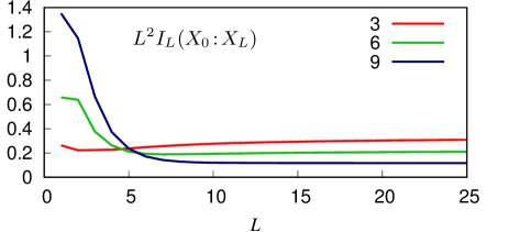
Figure 4: $L^{2}I_{L}(X_{0}\!:\!X_{L})$, the end-to-end mutual information multiplied by $L^{2}$ for the exceptional cases of odd-${\cal N}$, $C\in 3{\mathbb{N}}$, which have zero-energy modes Nourhani et al. (2018).

Recall that ${\cal N}_{c}$ (30) is the number of modes of non-negative energy, hence including the zero-energy modes. For any configuration $X_{0}$ at $\tau=0$ with ${\cal N}(X_{0})\geq{\cal N}_{c}=C/3+1$, there is a finite relaxation (imaginary) time $\tau_{0}$, such that for $\tau_{0}\ll\tau\ll L$, the state is nearly certain to be in the lowest energy state of ${\cal N}_{c}$ particles, which has all single-particle modes up to and including the zero-energy modes occupied. The transition to ${\cal N}_{c}-2$ particle state without the zero-energy modes can take place anywhere along the length, or not at all, giving $L+1$ possibilities which all have equal entropy. Essentially those are the only states of the entire cylinder in play, and the probability that the transition does not occur is proportional to $1/L$. If, on the other hand, the “initial” state has only ${\cal N}_{c}-2$ particles, then the transition is impossible, of course, but there is no entropy penalty for this case compared to transitioning from ${\cal N}_{c}$ to ${\cal N}_{c}-2$ at any particular location. By this reasoning, we arrive at the following simplified model. The number of occupied zero modes at the top of the cylinder is $N_{t}$ and the number at the bottom is $N_{b}$. They are restricted according to $N_{t},N_{b}\in\{0,2\}$ and $N_{b}\leq N_{t}$. $N_{b}<N_{t}$ means there is a “domain wall” somewhere in the system. The possibilities of no domain wall and one between rings $n$ and $n+1$ for each $n$ are all equiprobable, with probability $1/L$. Joint and marginal probabilities of $N_{t}$ and $N_{b}$ are recorded in the following table.

	0	2
0	$\;1/L$	$1-2/L$	$1-1/L$
2	$\;0$	$1/L$	$1/L$
	$\;1/L$	$1-1/L$

The computation of mutual information proceeds as follows, and involves some perhaps unexpected cancellation.

$$I(N_{b}\!:\!N_{t})= H(N_{b})-P(N_{t}=0)H(N_{b}\!:\!N_{t}=0)$$

$$-P(N_{t}=2)H(N_{b}\!:\!N_{t}=2)$$

$$= -\left(1-\frac{1}{L}\right)\ln\left(1-\frac{1}{L}\right)-\frac{1}{L}\ln\frac{1}{L}$$

$$+\left(1-\frac{2}{L}\right)\ln\left(\frac{1-\frac{2}{L}}{1-\frac{1}{L}}\right)+\frac{1}{L}\ln\frac{\frac{1}{L}}{1-\frac{1}{L}}$$

$$= -2\left(1-\frac{1}{L}\right)\ln\left(1-\frac{1}{L}\right)$$

$$+\left(1-\frac{2}{L}\right)\ln\left(1-\frac{2}{L}\right)$$

$$=L^{-2}+{\cal O}(L^{-3}).$$ (62)

The inverse-square falloff of mutual information is now explained.

5 Conclusion

The disorder of the zero-temperature TIAFM is similar in some way to the standard Perron-Frobenius scenario for thermal disorder, but very different in others, and the latter are not difficult to find. The fermionic formulation makes clear the origin of the abnormalities — it is the semi-conservation of particle number, and it facilitates detailed computations. For a cylindrical system, mutual information is a natural tool to study the dependence of the complex composite degrees of freedom comprised by spins in a ring. Zero-temperature pure phases for infinite cylinders are relatively normal compared to thermally disordered states: the transfer matrix recovers transitivity, albeit on a reduced configuration space labelled by total particle number ${\cal N}$. Yet the very existence of multiple phases is abnormal. The falloff rate of the ring-to-ring mutual information is twice that of correlation functions, the latter equal to the spectral gap. End-to-end mutual information on finite cylinders, by contrast, deviates significantly from expectations for a disordered spin system in complex dependence on circumference and periodicity or antiperiodicity. These phenomena are, however, easily understood in terms of energies of single particle states in a noninteracting fermi system.