Triangular Ising antiferromagnet through a fermionic lens, part 1:
free energy, zero-temperature phases and spin-spin correlation

Abstract

We develop a fermionic formulation of the triangular lattice Ising antiferromagnet (TIAFM) which is both calculationally convenient and intuitively appealing to imaginations steeped in conventional condensed matter physics. It is used to elucidate a variety of aspects of zero-temperature models. Cylindrical systems possess multiple “phases” distinguished by the number of circumferential satisfied bonds and by entropy density. On the plane, phases are labelled by densities of satisfied bonds of two different orientations. A local particle (semi)conservation law in the fermionic picture lies behind both these features as well as the classic power-law falloff of the spin-spin correlation function, which is also derived from the fermionic perspective.

I Introduction

Classical Ising spin models with nearest-neighbor interactions are archetypes of many fundamental phenomena of statistical mechanics. For instance, the square-lattice model with ferromagnetic couplings, favoring all spins alike, exemplifies order-disorder transitions, spontaneous symmetry breaking, and via Onsager’s exact solution Onsager (1944), “nonclassical” critical phenomena. Qualitatively, a ferromagnetic model on any lattice behaves similarly. At the level of thermodynamic functions, so do antiferromagnetic models on bipartite lattices, such as square or hexagonal, since they also have two ground states with every bond satisfied (i.e., in its low-energy configuration). The antiferromagnetic model on a triangular lattice behaves entirely differently. Even at zero temperature, it fails to order, because there is no spin configuration that satisfies all three bonds around any elementary triangle.

As the simplest model with this property, the triangular Ising antiferromagnet (TIAFM) is the archetype of (geometric) frustration (Toulouse Toulouse (1977) credits P. W. Anderson with the coinage). Frustration, simply the presence of incompatible but equally strong elementary interactions, occurs in an enormous range of systems, from water ice Pauling (1935); Giauque and Stout (1936) to spin systems Toulouse (1977); Moessner (2001); Normand (2009); Gingras and McClarty (2014); Starykh (2015); Schmidt and Thalmeier (2017), artificial spin ice Wang et al. (2006); Zhang et al. (2012); Perrin et al. (2016), colloidal assemblies Tierno (2016); Han et al. (2008), Coulomb liquids Mahmoudian et al. (2015), lattice gases Weigt and Hartmann (2003), ferroelectrics Choudhury et al. (2011), coupled lasers Nixon et al. (2013), and self-assembled lattices of microscopic chemical reactors Wang et al. (2016). One major consequence is a disordered macrostate with a nonzero entropy density even at zero temperature. However, the disorder in this state differs from ordinary thermal disorder in significant ways. For instance, the zero-temperature TIAFM exhibits rigidity in the sense that certain kinds of subconfigurations are not just unlikely, but forbidden. The system geometries we shall be concerned with are, as depicted in Fig. 1, flat on the top edge and serrated on the bottom. In such cases, each downward-pointing triangle ($\bigtriangledown$) must have precisely one unsatisfied bond in a ground microstate. As we explain later, there is no such restriction on upward-pointing triangles ($\bigtriangleup$’s) — they may well have three unsatisfied bonds. Millane and coworkers Millane and Blakeley (2004); Millane and Clare (2006); Blakeley and Millane (2006) have investigated this possibility of fully unsatisfied triangles in TIAFM ground microstates in a variety of finite systems. The local rigidity associated with the $\bigtriangledown$’s opens the door for boundary conditions to exert an infinite-range influence and the possibility of multiple zero-temperature phases.

We aim here to elucidate consequences of this local rigidity through exploitation of a simple equivalence between the zero-temperature TIAFM and a system of fermions evolving in imaginary time, expanding on a previous brief report Nourhani et al. (2018). We believe readers familiar with creation and destruction operators and the notion of a Fermi sea will find the resulting treatment intuitively appealing. In the fermionic representation, the zero temperature prohibition of $\bigtriangledown$’s with three unsatisfied bonds appears as a local semi-conservation of particles — “semi” because pairs of neighboring particles may annihilate. For cylindrical systems this leads to multiple phases characterized by the number of particles, equivalently, the number of satisfied circumferential bonds. Essentially, these phases are the string sectors of Ref. Dhar et al. (2000), which seem to have first appeared in the work of Blöte, Hilhorst and Nienhuis Blote and Hilhorst (1982); Nienhuis et al. (1984) connecting the TIAFM to solid-on-solid models for crystal surfaces. recover the formula of Dhar et al. Dhar et al. (2000) for the entropy density of these phases as function of particle density, by simply filling a Fermi sea.

Our approach also gives some new results for planar systems. Pure phases are labelled by the densities of satisfied bonds in two differing orientations; the density of satisfied bonds with the third orientation is then determined. The power law ($r^{-1/2}$) decay of the spin-spin correlator in the planar system at zero temperature, found by Stephenson Stephenson (1964, 1970), has an interpretation and derivation in terms of anomalously small fluctuations in the number of fermions in a segment. It is not hard to see that local particle conservation is a necessary condition for this. Otherwise, the fermionic ground state would inevitably have extensive root-mean-square number fluctuations, leading to exponential decay of the correlation.

Wannier Wannier (1950) obtained the free energy density of the isotropic TIAFM already in 1950 by adapting the method of Kaufman and Onsager Kaufman and Onsager (1949), but the zero-temperature limit reveals only the phase with highest entropy density Aizenman and Lieb (1981).

Section II presents full details of two reformulations of the TIAFM. First in terms of “strings”, a representation which can already provide some qualitative insight, but is not convenient for calculations. Second, interpreting the strings as worldlines of fermions, we obtain an appealing formulation drawing on familiar tools and concepts such as creation/destruction operators and Fermi seas, with which calculations can be carried out. The fermions are actually not so distant from the original model — they correspond directly to satisfied bonds along the spatial direction, which is circumferential on a cylinder. The bulk entropy densities of the zero-temperature phases for a cylinder are computed as energies of Fermi seas [Eq. (13) and Fig. 3]. Section II is assumed for all the other sections, as well as for the companion paper, Part 2. Otherwise, however, those are all independent. Section III turns from cylinders to parallelogram planar domains with toroidal-type boundary conditions (opposite edges match as in periodic boundary conditions, but may be constrained). Conservation of bond densities along all three orientations is shown. The result, apparently previously unnoticed, is that in the infinite-system limit there is a two-dimensional continuum of ground states characterized by the densities of unsatisfied bonds in the three orientations. We compute the entropy density as a function of the fraction of unsatisfied bonds. [Fig. 4 and Eq. (III)]. Section IV derives the asymptotic inverse-square-root decay of the spin-spin correlator along lattice directions within the fermionic model. Since it is directly related to fluctuations of the particle number in a segment of a ring, the particle conservation law is implicated in its behavior. A companion paper (Part 2) will explore the application of the fermionic perspective to information theoretic aspects of zero-temperature states on cylinders, both finite and infinite. The only part of this paper on which it depends is Section II.

II TIAFM on cylindrical domains

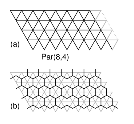
Figure 1: (a) A $\bigtriangledown$-type triangular lattice system. Identifying the vertices at the extreme left and right ends of the rows produces a cylinder with periodic spin boundary conditions. If the light gray bonds at the right edge have reversed (ferromagnetic) coupling sign, then wrapping into a cylinder is equivalent to antiperiodic spin boundary conditions. (b) The dual of the triangular lattice is the honeycomb lattice.

This section travels the road from TIAFM in its native formulation as a spin model to the equivalent fermion system, and makes the first use of the latter in a painless derivation of the zero temperature entropy densities for cylinders. We begin by considering constraints on bond microstates and their interplay with boundary conditions in the class of planar TIAFM fragments that decompose into down-pointing triangles. These are called “$\bigtriangledown$-type”, and $\bigtriangleup$-type is defined in an analogous way. We shall see that bond microstates can always be represented by “string diagrams” on the dual (honeycomb) lattice. This is crucial for our approach and is discussed in Section II.2. For systems on parallelograms or cylinders, which decompose into parallel strips or rings, respectively, the strings can be thought of as worldlines of particles, where the strips or rings correspond to the space at differing (imaginary) times. This observation inspires a fundamental analytical tool — a reformulation of cylindrical TIAFM systems as fermions on a ring. Although they do not interact in the usual sense, neighboring fermions can disappear, or annihilate, in pairs. (This of course involves a convention about the direction of time; under the opposite convention, they appear in pairs.) Annihilation events correspond exactly to $\bigtriangleup$’s with three unsatisfied bonds. For the most part, the ramifications of pair annihilation are pushed into the background until Part 2. We use the fermionic representation in this section to calculate the entropy densities of the pure phases on a cylinder. This entropy density is simply the energy of the corresponding Fermi sea, demonstrating both the intuitive appeal and calculational convenience of the fermionic formulation.

II.1 boundary conditions and bond microstates

In general, the naive rule that ground spin microstates have exactly one unsatisfied bond per elementary triangle is too restrictive Blakeley and Millane (2006); Millane and Clare (2006). This is because a bond usually belongs to two triangles, yet contributes to the energy only once. If a finite fragment of triangular lattice can be decomposed into a set ${\cal S}$ of triangles with no shared edges (but possibly shared vertices), then, with free boundary conditions, the ground microstates are precisely those with one unsatisfied bond in each triangle of ${\mathcal{S}}$. For example, consider the parallelepiped system shown in Fig. 1a. It can be decomposed into down-pointing triangles ($\bigtriangledown$), hence we say it is $\bigtriangledown$-type. However, it is not $\bigtriangleup$-type, since it does not decompose completely into non-edge-sharing $\bigtriangleup$’s. In fact, there are ground microstates in which some $\bigtriangleup$s contain three unsatisfied bonds. The cylinder constructed from such a parallelogram by imposing left/right periodic boundary conditions (along the horizontal rows) is still $\bigtriangledown$-type. So is the torus resulting therefrom by imposing periodicity in the vertical direction. The latter, however is also $\bigtriangleup$-type; the naive rule therefore applies in this last case. Cylinders are our primary interest; we will write $C$ for the (number of spins around the) circumference, and $L$ for the length (number of circumferential rings of spins).

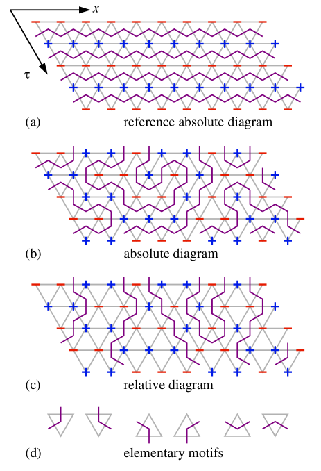
Figure 2: (a) The fiducial ground microstate, with all bonds non-vertical bonds satisfied (the dual bonds are indicated by heavy lines). (b) An absolute string diagram. (c) From the dual representation of any ground microstate, the string representation is constructed by an XOR operation with the fiducial microstate. Thus, vertical dual bonds along a string are dual to bad bonds, non-vertical to satisfied bonds. (d) Elementary string unit motifs.

For either a $\bigtriangledown$-type or $\bigtriangleup$-type system with open boundary conditions, the microstate with all horizontal bonds unsatisfied and non-horizontal bonds satisfied is a ground microstate. Such a microstate is represented in Fig. 2a. If periodic spin boundary conditions are imposed, however, this bond microstate may be spin-inconsistent, that is, unrealizable by any spin configuration. With periodic spin boundary conditions, the requirement for spin-consistency is that around every closed loop the number of satisfied bonds is even. However, if this checks for each elementary triangle and for one loop around each periodic direction, then it automatically holds for any other loop. Under antiperiodic spin boundary conditions, on the other hand, a loop around the periodic direction must contain an odd number of satisfied bonds. Periodic spin boundary conditions are naturally viewed as implemented by literally wrapping the system into a cylinder, so that spins at the left and right ends of the rows [as in Fig. 1(a)] become identified. At first sight, antiperiodic spin boundary conditions seem artificial. However, they are easily implemented by reversing the signs of the couplings on the zig-zag row of bonds comprised by the tops and right sides of the $\bigtriangledown$s at the right ends of the rows (light gray in Fig. 1a) before wrapping into a cylinder.

Equally important is that we can proceed without explicit mention of spins at all. Henceforth bonds are regarded as fundamental. The parity (even or odd) of the number of satisfied bonds on a loop around a periodic direction will need to be specified either explicitly or implicitly via bond boundary conditions. We shall also consider more general boundary conditions than familiar simple periodic boundary conditions. Simple periodic boundary conditions require, for example, the bond configuration on the right edge of a parallelogram as in Fig. 1a to match that on the left, and nothing more. Since there are no actual bonds on the right edge, what is really meant here is whether pairs of neighboring spins agree or disagree. Generalized periodic boundary conditions means a periodicity constraint of that sort, plus, potentially, others. For instance, we may specify exactly what the bond configuration is.

II.2 from bond microstates to strings and particles

The dual $G^{*}$ of a graph $G$ is obtained by regarding the faces of $G$ as vertices of $G^{*}$ and “sharing an edge” in $G$ as the neighbor relation in $G^{*}$. Working on the dual lattice can reveal connectivity structures which are less obvious on the original Baxter (2007). As shown in Fig. 1b, the dual of a patch of triangular lattice is a patch of honeycomb lattice. The bond dual to a triangular lattice bond is just the honeycomb edge crossing it. An absolute string diagram is derived from a bond microstate as all the bonds dual to satisfied bonds, thought of as connected when they share a vertex. For a general system in any microstate, each triangle has either zero or two satisfied bonds; the corresponding string diagram therefore consists of continuous chains (“strings”) of dual bonds, which cannot end anywhere inside the system; loops, however, may be present. As shown in Fig. 2b, the string diagrams for ground-microstates of a $\bigtriangledown$-type system are precisely those for which every $\bigtriangledown$  is crossed by a string, while $\bigtriangleup$’s may or may not be crossed.

In the following, we will be using relative string diagrams rather than absolute ones. Given a reference string diagram, a second is converted to a relative one by an exclusive or operation (XOR) with the reference, i.e., the dual bonds occurring in one or the other but not both, are selected. A relative string diagram also consists of strings which do not end inside the system. Our reference string diagrams are of the form shown in Fig. 2a, zig-zagging all the way across the system; this corresponds to all spins up in one row, down in the next, and so forth. Diagrams relative to that reference do not have loops, as we now show. Since a $\bigtriangledown$ has exactly one unsatisfied bond, the only freedom we have is to move it, or equivalently swap it with one of the satisfied bonds. This gives rise to one of the first two motifs in Fig. 2d. Since the $\bigtriangleup$’s also have one unsatisfied bond in the reference microstate, we have the same options with these, giving the third and fourth motifs. Because the sytem is $\bigtriangledown$-type, $\bigtriangleup$’s with three unsatisfied bonds corresponding to the motif are allowed, but $\bigtriangledown$’s with three unsatisfied bonds () are not. With the allowed palette of motifs, there is no way to make a closed loop since would have to occur at each locally highest point. An example of a relative string diagram constructed in the described way is shown in Fig. 2c. Note that vertical segments on the diagram correspond to satisfied bonds, slanted segments to unsatisfied bonds.

II.3 spinless fermion implementation

To get from string diagrams to the fermionic formulation, interpret the strings as worldlines of particles, with the horizontal direction being position $x$ and imaginary time $\tau$ increasing downward. Integer times coincide with rows of horizontal bonds and integer positions with the centers of the bonds; constant $x$ shifts to the right in Fig. 2c as $\tau$ increases. Then, for all $\tau$, allowed particle positions take values in ${\mathbb{Z}}_{C}$, the integers modulo $C$, that is, $\{0,1,\cdots,C-1\}$ with $(C-1)+1$ identified with $0$, etc.

With open boundary conditions, particles can hop off the spatial lattice completely. Otherwise, the only way for them to disappear is via pair annihilation events; one such appears in Fig. 2c. Thus, a local semi-conservation law for particle number is in effect — particles can disappear from a region through pair annihilation, but can appear only by moving through the boundary. When left/right generalized periodic boundary conditions are imposed, it is no longer possible for a string to exit left or right. It must wrap around. The particular string diagram in Fig. 2c contains a feature which is interpreted, under open boundary conditions, as a particle leaving the system at left and another entering at right, but under generalized periodic boundary conditions, simply as a particle wrapping around. If periodic boundary conditions are applied also in $\tau$, possibly with a spatial twist, the strings must match up, top and bottom; this implies that the number of strings must be the same on every time-slice, so that annihilation events are forbidden.

For the remainder of this section, we restrict attention to particle-conserving microstates, i.e., there are the same number (${\cal N}$) of strings entering the top of the system as exit the bottom. This can be enforced by bond boundary conditions even weaker than generalized periodic. With no annihilation events, each particle either stays at the same position or moves one to the left as $\tau$ increases by one unit, but each site can hold only one. A way to implement this restriction without an interaction is to take the particles to be spinless fermions, thereby embedding the classical statistical mechanical problem in a quantum mechanical problem. A particle configuration $X=(x_{1},\ldots,x_{\cal N})$ is just a set of positions. By convention, we assume they are ascending order: $0\leq x_{1}<x_{2}<\ldots<x_{\cal N}\leq C-1$. The particle state space then consists of probability measures over the configuration space ${\cal X}$. If we overload the symbol ‘$X$’ by using it to also denote a probability measure giving probability 1 to configuration $X$, the general element of ${\cal X}$ can be written as

$$\mu=\sum_{X\in{\cal X}}\mu(X)X.$$

We embed this state space into the fermionic Fock space as

$$X=(x_{1},\ldots,x_{\cal N})\mapsto\Psi(X)=c_{x_{1}}^{\dagger}\cdots c_{x_{\cal N}}^{\dagger}|{\varnothing}\rangle,$$ (1)

and extend linearly to mixtures:

$$\Psi(\mu)=\sum_{X\in{\cal X}}\mu(X)\Psi(X).$$

To avoid spurious minus signs due to fermionic statistics, scrupulous adherence to the operator ordering convention in (1) is crucial.

Now we construct the particle-number conserving transfer matrix ${\mathbb{T}}_{0}$. For a particle at site $x$ at time $\tau$, there are two options for its position at time $\tau+1$: $x$ or $x-1$ (see Fig. 2b). Thus, we want ${\mathbb{T}}_{0}$ to act as

$${\mathbb{T}}_{0}\,c_{x_{1}}^{\dagger}\cdots c_{x_{\cal N}}^{\dagger}|{\varnothing}\rangle=(c_{x_{1}-1}^{\dagger}+c_{x_{1}}^{\dagger})\cdots(c_{x_{\cal N}-1}^{\dagger}+c_{x_{\cal N}}^{\dagger})|{\varnothing}\rangle.$$

Due to the very short range of hopping, any term occuring in the expansion of the right-hand side will have particles inserted in the right order, at least up to cycling around the ring. The possibility $x_{1}=0$ requires an additional condition. Since

$$c_{x_{1}}^{\dagger}\cdots c_{x_{\cal N}}^{\dagger}|{\varnothing}\rangle=(-1)^{{\cal N}-1}c_{x_{2}}^{\dagger}\cdots c_{x_{\cal N}}^{\dagger}c_{x_{1}}^{\dagger}|{\varnothing}\rangle,$$ (2)

we take $c_{j+C}=-c_{j}$ in the even-${\cal N}$, and $c_{j+C}=c_{j}$ in the odd-${\cal N}$ sector. This condition avoids spurious minus signs from fermionic statistics, and and is compatible with pair annihilation since the latter conserves particle number mod 2.

Therefore, the conditions to be imposed on ${\mathbb{T}}_{0}$ are

$${\mathbb{T}}_{0}c_{x}^{\dagger}=(c_{x-1}^{\dagger}+c_{x}^{\dagger}){\mathbb{T}}_{0},\quad{\mathbb{T}}_{0}|{\varnothing}\rangle=|{\varnothing}\rangle.$$ (3)

However, there is no point in solving this directly in position space. Since the transfer matrix is translation invariant, we immediately pass to $k$-space, using

$$c(k)^{\dagger}=\frac{1}{\sqrt{C}}\sum_{x\in{\mathbb{Z}}_{C}}e^{ikx}c_{x}^{\dagger}.$$ (4)

Then, our condition (3) is rewritten as

$${\mathbb{T}}_{0}c(q)^{\dagger} ={C}^{-1/2}\sum_{x\in{\mathbb{Z}}_{C}}e^{iqx}{\mathbb{T}}_{0}c_{x}^{\dagger}$$ (5)

$$=\left(2\cos\frac{q}{2}\right)e^{iq/2}{c}(q)^{\dagger}{\mathbb{T}}_{0}.$$

From this, we deduce that

$${\mathbb{T}}_{0}=\prod_{k\in{\mathrm{BZ}}}\left[1-n(k)+\left(2\cos\frac{k}{2}\right)e^{ik/2}n(k)\right],$$ (6)

in terms of the occupation number operators $n(k)=c(k)^{\dagger}c(k)$. Here,

$$\mathrm{BZ}=\begin{cases}\frac{2\pi}{C}\cdot{\mathbb{Z}}\cap(-\pi,\pi],&{\cal N}\,\mathrm{odd}\\ \frac{2\pi}{C}\cdot\left({\mathbb{Z}}+\frac{1}{2}\right)\cap(-\pi,\pi],&{\cal N}\,\mathrm{even}.\end{cases}$$ (7)

Since the $n(k)$ are idempotent and commute, ${\mathbb{T}}_{0}$ can be rewritten as

$${\mathbb{T}}_{0}=e^{-{H}_{0}+iP/2},$$ (8)

where

$${H}_{0}=\sum_{q\in\mathrm{BZ}}{\varepsilon}(q)n(q),\qquad P=\sum_{q\in\mathrm{BZ}}q\,n(q),$$ (9)

can be considered a Hamiltonian and total momentum operator, respectively, with an effective mode energy

$${\varepsilon}(q)=-\ln\left(2\cos\frac{q}{2}\right).$$ (10)

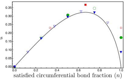
Figure 3: Zero-temperature entropy per spin of the cylindrical TIAFM as function of satisfied circumferential bond fraction (equal to particle density in the fermionic picture). Solid curve: $C\to\infty$ limit, given by the formula in Eq. (13). Symbols: exact numerical results for circumference 3 ($\square$), 4 ($\diamondsuit$) and 8 ($\triangledown$). Solid (open) symbols denote periodic (antiperiodic) boundary conditions. Except at $n=1$, for which entropy density is exactly $(\ln 2)/C$, the $C=\infty$ limit is nearly attained already for $C=8$. Nourhani et al. (2018)

The band velocity

$$v(q)=\frac{\partial{\varepsilon(q)}}{\partial{q}}=\frac{1}{2}\tan\frac{q}{2}$$ (11)

is a normal dispersion relation insofar as it is monotone increasing with $q$ and $v(0)=0$. However, it has the peculiarity that $\varepsilon(\pi)=+\infty$. According to (7), this value occurs for ${\cal N}$ and $C$ of opposite parity. Momentum $\pi$ is allowed, but is immediately killed by the $\tau$-evolution ${\mathbb{T}}_{0}$. Although peculiar, this is not cause for alarm; no matter the number of particles, they can be accomodated without occupying the $\pi$ mode. The ground states of $H_{0}$ are simply filled Fermi seas — all modes with momentum of absolute value not exceeding the Fermi momentum $k_{F}$ are occupied. Since a $q=0$ state is available for odd, but not even, particle number [see Eq. (7)], we construct a ground state by occupying $q=0$ in case ${\cal N}$ is odd and then, whether ${\cal N}$ is odd or even, occupying the $q$ and $-q$ modes in pairs for increasing $q$. The only potential source of ground-state degeneracy is the occurence of modes with $\varepsilon(q)=0$, which is equivalent to $|q|=2\pi/3$. From (7) and (9), such modes occur only for odd ${\cal N}$ and $C\in 3{\mathbb{N}}$. These cylinders turn out to have a number of unusual properties due to the existence of zero-energy modes; they which will be explored later.

We can now easily compute the entropy density $\sigma$ for the cylinder of circumference $C$ and length $L$, asymptotically as $L\to\infty$ and $C\to\infty$, if the boundary conditions (at top and bottom) are particle number conserving:

$$e^{CL\sigma}=\mathrm{Tr}_{\cal N}{\mathbb{T}}_{0}^{L}=\sum_{E\in\,\mathrm{spec}\,H_{0}}e^{-EL}\sim e^{-E_{0}(n)L},$$ (12)

where $E_{0}(n)$ is the ground state of the fermion system at density $n$. Since the Fermi momentum is $k_{F}=\pi n$, the asymptotic entropy density is

$$\sigma=-\frac{E_{0}}{C}=-\int_{0}^{k_{F}}\varepsilon(q)\,\frac{dq}{\pi}.$$ (13)

This formula was previously given by Dhar et al. Dhar et al. (2000) in a bare mathematical form. Fig. 3 shows the entropy density as a function of the fraction, $n$ of satisfied horizontal bonds. Also shown there are numerical results for small values $C=3,4$ and 8. For finite $C$, the integral in (13) should be replaced by a sum. From the figure, there is very little difference already for $C=8$. The maximum entropy density is attained at $\overline{n}(-)=1/3$, as expected, since that is the “natural” value (1/3 of the bonds of each orientation unsatisfied).

II.4 cylinder phases

Now consider a sequence of arbitrary boundary conditions on cylinders of fixed circumference, with $\tau$ running from $-L_{t}$ to $L_{b}$ for $L_{t},L_{b}\to\infty$. Even without knowing quantitative details about how to incorporate pair annihilation into the transfer matrix, we can understand what limiting bulk states exist. Without any loss (as shall be clear, if not already), assume that the boundary conditions restrict the number of particles (satisfied bonds, recall) at the top of the cylinder to ${\cal N}$(top) and at the bottom to ${\cal N}$(bot). In order to have ground microstates, we require ${\cal N}$(top) $\geq{\cal N}$(bot). If ${\cal N}$(top) $={\cal N}$(bot) $={\cal N}$, then the bulk state is simply the state the entropy of which was just calculated. Since the transfer matrix acts irreducibly on the ${\cal N}$-satisfied-bond configuration space, there can be only one ${\cal N}$ particle bulk state. We call these the (zero-temperature) pure phases, since they play the same role as more ordinary pure phases do at positive temperature. Now, if ${\cal N}$(top) $>{\cal N}$(bot), then the particle number can decrease from top to bottom. In the limit $L_{t},L_{b}\to\infty$, the bulk will be found in the pure phase with a particle number ${\cal N}$(bulk), satisfying ${\cal N}$(bot) $\leq{\cal N}$(bulk) $\leq{\cal N}$(top) and maximizing $\sigma({\cal N}(\text{bulk})/C)$ (equivalently, minimizing the energy of the Fermi sea), if such is unique. It the maximum of $\sigma$ is reached at two accessible values, then the limiting bulk state will be a probabilistic mixture of the two pure phases. There is no way to localize a domain wall. Given any finite region $-L_{0}<\tau<L_{0}$, the probabilities that the domain wall will be above or below the region in the limit $L_{t},L_{b}\to\infty$ depends on details of the sequence of values of $L_{t}$ and $L_{b}$, but it is inside the region with probability zero. Thus, all limiting states are simple probabilistic mixtures of pure phases. This contrasts with, for example, the two-dimensional ferromagnetic Ising model, for which interface states with a localized domain wall between up and down phases can be stabilized by boundary conditions below the roughening temperature. That, of course, is not surprising.

III two-dimensional continuum of planar ground macrostates

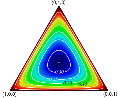
Figure 4: Colormap/contour plot of entropy density $s(\overline{n}(-),\overline{n}(/),\overline{n}(\backslash))$ as function of unsatisfied bond fractions $\overline{n}(-)$, $\overline{n}(/)$ and $\overline{n}(\backslash)$ in the three orientations, using barycentric coordinates. The vertices are labelled by the extreme unsatisfied bond fractions (all and only bonds with a particular orientation unsatisfied). Each point in the diagram is a convex sum of the vertices with coefficients $(\overline{n}(-),\overline{n}(/),\overline{n}(\backslash))$ satisfying $\overline{n}(-)+\overline{n}(/)+\overline{n}(\backslash)=1$. Fig. 3 is a slice through this plot along a line from a vertex to the midpoint of the opposite edge.

We have seen that by virtue of periodicity along the $x$ direction, cylindrical systems exhibits a semi-conserved quantity. The number of particles, equivalently the number of horizontal satisfied bonds, cannot increase from row to row. In fact, the semi-conservation law holds for any microstate which respects periodicity. Thus, any boundary conditions matching left and right edges (generalized periodic) preserves its validity. Suppose we have such left-to-right generalized periodic boundary conditions, and additionally impose similar boundary conditions forcing the top and bottom to match. In that case, as already discussed, the semi-conservation of unsatisfied bond number along horizontal rows is promoted to a conservation law. Now, by vitue of top-bottom matching, the numbers of unsatisfied bonds along rows parallel to the left or right edge are also all the same — a second “conservation” law. This can also be seen directly from the particle picture as follows. The boundary conditions mean that particles may enter the system at some positions at $\tau=0$ as long as an equal number (not necessarily the same ones!) are removed from the same positions at $\tau=L$. The net current into the system between $\tau$ and $\tau+1$ is controllable, but we are not allowed to change the particle number in the system, so if a particle is put in on the right, another must be simultaneously taken out on the left. It follows, then, that the net number of particles crossing a given $x$ position during the interval $[0,\tau]$ is the same for each position. If it were not, particles would build up somewhere and it would be impossible to extract them at $\tau=L$ from the same positions as they were injected at $\tau=0$.

This means that there is a two-dimensional continuum of boundary-controllable ground states. But how is the new conserved quantity represented in the particle implementation? How can we calculate the entropy with both unsatisfied bond fractions constrained? It is not straightforward to work with a direct constraint on the net current. Instead, we will use simple periodic boundary conditions and couple an external field to the current. This will deliver a Legendre transform of the entropy. Thus, we generalize the transfer operator ${\mathbb{T}}_{0}$ to

$${\mathbb{T}}_{\alpha}=\prod_{i\in{\mathbb{Z}}_{C}}(1+e^{-\alpha}c_{i-1}^{\dagger}c_{i}),\quad\alpha\in{\mathbb{R}}.$$ (14)

Adjusting $\alpha$ gives greater weight to jumps in one direction or the other. As before, we compute

$${\mathbb{T}}_{\alpha}\,c(q)^{\dagger}=\left(2\cos\frac{q+i\alpha}{2}\right)e^{i(q+i\alpha)/2}{c}(q)^{\dagger}{\mathbb{T}}_{\alpha}.$$ (15)

According to (14), $\alpha$ is coupled only to the “left-moving” current. It makes no essential difference to the end results, but we prefer to couple instead to the difference of right-moving and left-moving. This can be accomplished by multiplying ${\mathbb{T}}_{\alpha}$ by $e^{\alpha{\cal N}/2}$; the effect of this is just to remove the $i\alpha$ from the exponential in (15). With that adjustment, we find the $\alpha$-dependent pseudo-energy [cf. (10)]

$$\varepsilon_{\alpha}(q)=-\ln\left(2\cos\frac{q}{2}\cosh\frac{\alpha}{2}-2i\sin\frac{q}{2}\sinh\frac{\alpha}{2}\right),$$ (16)

which obeys $\varepsilon_{\alpha}(-q)=\overline{\varepsilon_{\alpha}(q)}$, and $\partial(\mathrm{Re}\,\varepsilon_{\alpha}(q))/\partial q$ has the same sign as $q$. Thus, with $k_{F}$ determined as before, the logarithm of the partition function in the presence of $\alpha$ is

$${\ln Z_{{}_{CL}}(n,\alpha)}=\sum_{|q|<k_{F}}\ln\left[1+e^{(\mu-\varepsilon_{\alpha}(q))L}\right].$$ (17)

Dividing by the system size, $CL$, and taking the thermodynamic limit here yields a Legendre transform $s(n,\alpha)$ of the entropy density (a “free entropy”):

$$\lim_{C,L\to\infty}\frac{1}{CL}\ln Z_{{}_{CL}}(n,\alpha) =-\int_{0}^{k_{F}}\mathrm{Re}\,\varepsilon_{\alpha}(q)\,\frac{dq}{\pi}$$

$$=s(n,\alpha)$$

$$=\sigma(n,J)+\alpha J,$$ (18)

where the expected value of current density is related to $\alpha$ by

$$J=\frac{\partial{s}}{\partial{\alpha}}.$$ (19)

$\sigma(n,J)$ here is essentially what we want, except that one lattice direction is singled out as ‘$x$’, so that $n$ is the density of satisfied horizontal bonds, while those of the other two orientations are related to $J$. To treat them on an equal footing we use the expressions

$$\overline{n}(-) =1-n,\quad\overline{n}(/)=\frac{n}{2}+J,$$

$$\overline{n}(\backslash) =\frac{n}{2}-J.$$ (20)

for the fractions ($\overline{n}(\cdot)$) of unsatisfied bonds in the three orientations in terms of particle density and average current. These unsatisfied bond fractions range over the interval $[0,1]$ subject to the constraint $\overline{n}(-)+\overline{n}(/)+\overline{n}(\backslash)=1$. Using barycentric coordinates, Fig. 4 plots the entropy density as a function of $(\overline{n}(-),\overline{n}(/),\overline{n}(\backslash))$ as determined from $\sigma(n,J)$ by numerical evaluation of (20).

IV spin-spin correlator

IV.1 the general idea

Zero temperature is a critical point of the TIAFM in the sense that the correlation length is infinite so that the spin-spin correlation function decays with a power law rather than exponentially. Asymptotically, if $\hat{e}$ is the vector from a site to a nearest neighbor, then

$$\langle\sigma_{i}\,\sigma_{i+\ell\hat{e}}\rangle\sim\ell^{-1/2}\cos n\ell$$ (21)

In this section, we will examine this spin-spin correlator from the fermionic perspective. Our treatment has similarities to that of Villain and Bak Villain and Bak (1981).

Taking $\hat{e}$ along the circumferential direction and remembering that a vertical string segment represents a satisfied bond, we have

$$\sigma_{i}\sigma_{i+\ell{\hat{e}}}=e^{i\pi N_{\ell}},$$

where

$$N_{\ell}{\kern 1.99997pt}:{\kern-5.0pt}={\kern 1.99997pt}\sum_{j=1}^{\ell}n_{j}$$ (22)

is the number of particles in the segment $[1,\ell]$ at some fixed time. Then,

$$\langle\sigma_{i}\sigma_{i+\ell{\hat{e}}}\rangle=\left\langle e^{i\pi N_{\ell}}\right\rangle,$$ (23)

where the brackets on the left denote the statistical expectation in the spin model and those on the right, expectation in the filled Fermi sea state $\Omega$.

$N_{\ell}$ is transformed to momentum representation according to

$$\rho(k)=\sum_{x}e^{-ikx}n_{x},\quad n_{x}=\frac{1}{C}\sum_{x}e^{ikx}\rho(k),$$ (24)

yielding

$$N_{\ell}=\frac{1}{C}\sum_{k\in\mathrm{BZ}}\rho(k)\sum_{x=1}^{\ell}e^{ikx}={\ell}n+\tilde{N}_{\ell},\quad$$ (25)

where

$$\tilde{N}_{\ell}=\frac{1}{C}\sum_{k\in{\mathrm{B}Z}\setminus 0}w(k)\rho(k),$$ (26)

is the fluctuation part of $N_{\ell}$, and

$$w(k)=e^{ik(\ell+1)/2}\,\frac{\sin{k\ell}/{2}}{\sin{k}/{2}}.$$ (27)

Both $N_{\ell}$ and $\tilde{N}_{\ell}$ are bounded hermitian operators, so the expansion

$$\left\langle e^{i\theta\tilde{N}_{\ell}}\right\rangle=1+i\theta\langle\tilde{N}_{\ell}\rangle-\frac{1}{2}\theta^{2}\langle\tilde{N}_{\ell}\tilde{N}_{\ell}\rangle+\cdots$$ (28)

is legitimate. Since $\Omega$ has a definite momentum, $\langle\tilde{N}_{\ell}\rangle=0$. Evidently, the mean-square fluctuation $\langle\tilde{N}_{\ell}\tilde{N}_{\ell}\rangle$ of the particle number is important. Let us calculate it now, in the thermodynamic limit $C\to\infty$.

Acting on $\Omega$, $\rho(q)$ creates particle-hole excitations of momentum $-q$, $|q|/(2\pi/C)$ distinct ones if $|q|$ is small, but never more that $k_{F}C/\pi$. Then, $\langle\rho(-q^{\prime})\rho(q)\rangle=\langle\rho(q^{\prime})\Omega|\rho(q)\Omega\rangle$ is zero unless $q=q^{\prime}$ and then,

$$q<2k_{F},2(\pi-k_{F})\;\Rightarrow\;\langle\rho(-q)\rho(q)\rangle=\frac{C|q|}{2\pi}.$$ (29)

Therefore,

$$\langle\tilde{N}_{\ell}\tilde{N}_{\ell}\rangle\lesssim\frac{1}{C}\sum_{q\in{\mathrm{B}Z}\setminus 0}\frac{|q|}{2\pi}|w(q)|^{2}\,\stackrel{{\scriptstyle L\to\infty}}{{\longrightarrow}}\,\frac{1}{2\pi}\int_{0}^{\pi}q|w(q)|^{2}\frac{dq}{\pi},$$ (30)

the inequality arising because the contribution of large $|q|$ is overestimated. We compute a slightly more general integral, with a variable upper limit (in order to more clearly see which momenta contribute significantly):

$$I(\Lambda,\ell) =\int_{0}^{\Lambda/2}|w(k)|^{2}k\,dk$$ (31)

$$=4\int_{0}^{\Lambda/2}\sin^{2}{\ell x}\,\frac{x\,dx}{\sin^{2}{x}}$$

$$=4\int_{0}^{\ell\Lambda}\frac{\sin^{2}y}{y}\,dy+4\int_{0}^{\Lambda}x\theta(x)\sin^{2}{\ell x}\,dx.$$

In the final line, the singularity of $(\sin x)^{-2}$ was isolated by writing $(\sin x)^{-2}=x^{-2}[1+x^{2}\theta(x)]$ with $\theta:[0,\pi/2]\rightarrow[0,1-(2/\pi)^{2}]$ a monotone continuous function; the result was split into two integrals and the integration variable changed to $y=\ell x$ in the first. The second integral is clearly ${\mathcal{O}}(1)$ as $\ell\to\infty$. As for the first, a $\ln\ell$ behavior is vaguely discernible already at this point. To flush it out, split the integration range and apply a double-angle to obtain

$$\int_{0}^{\ell\Lambda}\frac{\sin^{2}y}{y}\,dy=\int_{0}^{\Lambda}\frac{\sin^{2}y}{y}\,dy+\frac{1}{2}\int_{\Lambda}^{\ell\Lambda}\frac{dy}{y}-\frac{1}{2}\int_{\Lambda}^{\ell\Lambda}\cos 2y\frac{dy}{y}$$

The second integral on the right is the important one; it evaluates to $\ln\sqrt{\ell}$. The first integral is clearly ${\mathcal{O}}(1)$. As for the third, an integration by parts yields

$$\int_{\Lambda}^{\ell\Lambda}\cos 2y\,\frac{dy}{y}=\frac{\sin 2y}{2y}\Big{|}_{\Lambda}^{\Lambda\ell}+\frac{1}{2}\int_{\Lambda}^{\Lambda\ell}\frac{\sin 2y}{y^{2}}\,dy={\mathcal{O}}(1).$$

An explicit integration and an integration by parts has been performed in passing to the second line. The second term there is a finite constant, the third term is manifestly ${\mathcal{O}}(1)$ as $\ell\to\infty$, and so is the last integral, since the integrand can be bounded in absolute value by $y^{-2}$. Finally, then, we find

$$I(\Lambda,\ell)=2\ln\ell+{\mathcal{O}}(1)\quad{\mbox{as}}\;\;\ell\to\infty.$$ (32)

There is here a breakdown of central limiting behavior — at least in one sense. Ordinarily, we would expect the mean-square number fluctuation to be proportional to the size of the subsystem, here $\ell$. However, the fluctuations actually turn out to grow much less rapidly than that. Nevertheless, it is still plausible that central limiting behavior obtains in another sense. If, for any particular large $\ell$, $\langle\tilde{N}_{\ell}\tilde{N}_{\ell}\rangle$ is the result of many weakly-dependent “modes”, then the fluctuations will be approximately normal, regardless of how the number and strength of the modes varies with $\ell$. [Consider, for example, a fixed quantity of a classical gas in volume $(N+1)V$ with $1\ll N$. The number fluctuations in some subvolume $V$ and of the remaining $NV$ have gaussian distributions with the same variance.] Assuming, then, that $\tilde{N}_{\ell}$ really does have an approximately Gaussian distribution, and looking at (28) as its characteristic function (in the probability theory sense),

$$\left\langle e^{i\theta N_{\ell}}\right\rangle \sim e^{in\theta\ell}\left\langle e^{i\theta\tilde{N}_{\ell}}\right\rangle$$

$$\sim e^{in\theta\ell}e^{-\frac{\theta^{2}}{2}\langle\tilde{N}_{\ell}\tilde{N}_{\ell}\rangle}\sim e^{in\theta\ell}(\sqrt{\ell})^{\theta^{2}/\pi^{2}}.$$ (33)

Setting $\theta$ equal to $\pi$, we recover (21). However, this rests on an assumption which has not been entirely justified — we need to verify the existence of many weakly independent modes which produce a Gaussian distribution of number fluctuations. That will be corrected in the next section. Before turning to that, note that a more ordinary central-limiting behavior of the number fluctuations, $\langle\tilde{N}_{\ell}^{2}\rangle\sim\ell$ would lead to an ordinary, noncritical exponential falloff of the spin-spin correlator.

IV.2 verifying Gaussianity

To get better control of $\langle e^{i\theta\tilde{N}_{\ell}}\rangle$, we split the number fluctuation into parts $\tilde{N}_{\ell>}$ and $\tilde{N}_{\ell<}$ containing the density modes with wavevectors in $(0,\pi)$ and $(-\pi,0)$, respectively. In order to relieve notational congestion, we shall henceforth omit the ‘$\ell$’ subscript on $N$; there is no danger of confusion. Noting that $\tilde{N}_{>}^{\dagger}=\tilde{N}_{<}$ and remembering that all the density modes commute, we have

$$\left\langle\Omega\,\Big{|}\,e^{i\theta\tilde{N}}\Omega\right\rangle=\left\langle e^{-i\theta\tilde{N}_{>}}\Omega\,\Big{|}\,e^{i\theta\tilde{N}_{>}}\Omega\right\rangle.$$ (34)

Proceed to examine the state $e^{i\theta\tilde{N}_{>}}\Omega$. The part, ${\mathcal{H}}$, of the fermion model Hilbert space which is relevant to us has a precise particle number (the size of the Fermi sea). This Hilbert space can be decomposed as ${\mathcal{H}}=\bigoplus_{n=0}^{\infty}{\mathcal{H}}_{n}$, according to the number of particle-hole excitations, $n$ (number of particles missing from the Fermi sea). Now, $\tilde{N}_{>}\,\Omega$ is in ${\mathcal{H}}_{1}$, of course. Applying a second fluctuation operator, we see that $\tilde{N}_{>}^{2}\,\Omega\in{\mathcal{H}}_{2}\oplus{\mathcal{H}}_{1}$; the second $\tilde{N}_{\ell}^{+}$ may create a second particle-hole pair, or it may move the already excited particle. The crucial point to note, though, is that the norm of the component in ${\mathcal{H}}_{1}$ is ${\mathcal{O}}(C^{-1})$ times that of the component in ${\mathcal{H}}_{2}$. This is because $\rho(q)$ can create $qC/2\pi$ distinct particle-hole excitations, but there is only one way it can boost the already excited particle. The argument just given can be applied over and over, showing that for any $m\ll C$, $(\tilde{N}_{>})^{m}\,\Omega$ is in ${\mathcal{H}}_{m}$, to relative order $C^{-1}$. Therefore, the component of $(\tilde{N}_{>})^{m}\,\Omega$ orthogonal to ${\mathcal{H}}_{m}$ is negligible in the thermodynamic limit.

It will now be useful to split a Fourier component $\rho(q)$ of the density as $\rho(q)=\rho(q)^{+}+\rho(q)^{-}+\rho(q)^{0}$, where $\rho(q)^{+}$ (the particle-hole creation part) contains the terms moving a particle from inside to Fermi sea to outside, $\rho(q)^{-}=[\rho(-q)^{+}]^{\dagger}$, those moving a particle from outside to inside, and $\rho(q)^{0}$ is the remainder. Correspondingly, we write

$$\tilde{N}_{>}^{+}=\frac{1}{C}\sum_{q>0}w(q)\rho(q)^{+},$$ (35)

and so forth. With this new notation, we can write the conclusion reached in the previous paragraph as

$$(\tilde{N}_{>})^{m}\,\Omega\simeq(\tilde{N}_{>}^{+})^{m}\,\Omega\in{\mathcal{H}}_{m},$$ (36)

where now we write ‘$\simeq$’ to mean ‘up to relative ${\mathcal{O}}(C^{-1})$’. Returning now to the inner product in (34) that we need to compute,

$$\left\langle e^{-i\theta\tilde{N}_{\ell}^{+}}\Omega\,\Big{|}\,e^{i\theta\tilde{N}_{\ell}^{+}}\Omega\right\rangle\simeq\sum_{m}\frac{(-\theta^{2})^{m}}{(m!)^{2}}\|(\tilde{N}_{>}^{+})^{m}\,\Omega\|^{2}.$$ (37)

It only remains to evaluate $\|(\tilde{N}_{>}^{+})^{m}\,\Omega\|^{2}=\langle(\tilde{N}_{>}^{+})^{m-1}\,\Omega\,|\,\tilde{N}_{<}^{-}(\tilde{N}_{>}^{+})^{m}\,\Omega\rangle$. By essentially the same reasoning leading to Eq. (29) for $\langle\rho(q)\rho(k)\rangle$, we have

$$[\rho(q)^{-},\rho(k)^{+}] \simeq\frac{Cc(q)}{2\pi}\delta(q,-k),$$

$$c(q) =|q|\;\;\mbox{if}\;\,|q|<2k_{F},2\pi-2k_{F}.$$ (38)

Insofar as the sought-for “many weakly dependent” modes are made explicit here, this is the linchpin of the calculation. Adding up over wavevector yields $[\tilde{N}_{<}^{-},\tilde{N}_{>}^{+}]\sim{I(\pi,\ell)}/{4\pi^{2}}$ and then

$$\tilde{N}_{<}^{-}(\tilde{N}_{>}^{+})^{m}\,\Omega\simeq m\frac{I(\pi,\ell)}{4\pi^{2}}(\tilde{N}_{>}^{+})^{m-1}\,\Omega.$$

A simple recursion now gives us

$$\|(\tilde{N}_{>}^{+})^{m}\,\Omega\|^{2}\sim m!\left(\frac{\ln\ell}{2\pi^{2}}\right)^{m}.$$ (39)

Substituting this into (37), the resulting series is recognizable as that of an exponential:

$$\left\langle e^{-i\theta\tilde{N}_{\ell}^{+}}\Omega\,\Big{|}\,e^{i\theta\tilde{N}_{\ell}^{+}}\Omega\right\rangle\sim\exp\left(-\frac{\theta^{2}}{2\pi^{2}}\ln\sqrt{\ell}\right).$$ (40)

This verifies Gaussianity, which is the final piece of the argument, according to the discussion just below Eq. (33).

V Conclusion

As one of the archetypal models of statistical mechanics, invoked in a wide variety of contexts, the triangular lattice antiferromagnetic Ising model deserves to be better understood outside the community of experts on exactly solvable models. The treatment given here should facilitate that, since it is based on an equivalence with more-widely-familiar and simple paradigms of solid-state physics. The fermionic formulation provides a fresh perspective and additional insight into the peculiarities of the zero-temperature states, showing them all be related to a (semi)conservation law for particle number.