Controlling spin supercurrents via nonequilibrium spin injection

Abstract

We propose a mechanism whereby spin supercurrents can be manipulated in superconductor/ferromagnet proximity systems via nonequilibrium spin injection. We find that if a spin supercurrent exists in equilibrium, a nonequilibrium spin accumulation will exert a torque on the spins transported by this current. This interaction causes a new spin supercurrent contribution to manifest out of equilibrium, which is proportional to and polarized perpendicularly to both the injected spins and equilibrium spin current. This is interesting for several reasons: as a fundamental physical effect; due to possible applications as a way to control spin supercurrents; and timeliness in light of recent experiments on spin injection in proximitized superconductors.

Introduction.— In the field of superconducting spintronics, a key objective is to study the interactions between superconductors (S) and ferromagnets (F) [1; 2; 3; 4]. These interactions produce new types of Cooper pairs $\ket{\uparrow\uparrow}$ and $\ket{\downarrow\downarrow}$ with a net spin polarization, which enables the use of S/F systems for dissipationless spin transport. From a fundamental physics perspective, such an interplay between different types of quantum order is expected to give rise to interesting physics to explore. Ultimately, the ambition is to exploit the interactions in S/F systems in devices related to e.g. supercomputing and ultrasensitive detection of heat and radiation.

One particular area that has attracted attention is how one may generate controllable spin supercurrents in equilibrium, either via inhomogeneous magnetism [5; 6; 7; 8; 9; 10] or spin–orbit coupling [11; 12; 13; 14]. In the magnetic case, it has been shown that two layers with noncollinear magnetic moments $\bm{m}_{{1}}$ and $\bm{m}_{{2}}$ give rise to an equilibrium spin supercurrent $\bm{J}_{\text{s}}^{\text{eq}}\sim\bm{m}_{{1}}\times\bm{m}_{{2}}$ [15]. While most work so far relies on magnetic control of spin supercurrents via rotation of $\bm{m}_{{1}}$ relative to $\bm{m}_{{2}}$, it would be interesting to determine if a spin supercurrent can be controlled via electronic spin injection instead. Such a mechanism might be more beneficial with regard to coupling superconducting and nonsuperconducting spintronics devices. Note that this is different from many previous works on spin injection in superconductors, which were largely explained in terms of quasiparticles and not a spin-triplet condensate [16; 17; 18; 19; 20; 21; 22].

Recently, there has been a renewed interest in using nonequilibrium spin injection as a means to manipulate spin supercurrents. This is largely due to a recent spin-pumping experiment [23], where microwaves were used to excite spins in the ferromagnetic layer of an N/S/F/S/N junction. This experiment showed that the pumped spin current could increase below the critical temperature $T_{\text{c}}$ of the S layers. It has been proposed that this effect was assisted by a Cooper-pair spin supercurrent [13], although alternative explanations have been proposed [24].

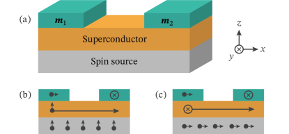
Figure 1: (a) Magnetic insulators with magnetizations $\bm{m}_{{{1}}}$ and $\bm{m}_{{{2}}}$ on a superconductor. In equilibrium, this yields a spin supercurrent $\bm{J}_{\text{s}}^{\text{eq}}\sim\bm{m}_{{{1}}}\times\bm{m}_{{{2}}}$. A spin source injects a spin accumulation $\bm{\rho}_{\text{s}}$, which exerts a torque on the spins transported by the equilibrium current, resulting in a new contribution ${\bm{J}_{\text{s}}^{\text{neq}}\sim\bm{\rho}_{\text{s}}\times(\bm{m}_{{{1}}}\times\bm{m}_{{{2}}})}$. (b) If the magnets are magnetized in the $x$- and $y$-directions, an equilibrium spin-$z$ supercurrent arises. Injection of spin-$z$ particles does not affect its polarization. Note that a spin supercurrent is in general a rank-2 tensor, which encodes both a polarization direction (short arrow) and transport direction (long arrow). (c) If spin-$x$ particles are injected, however, a new spin-$y$ supercurrent component is generated. Similarly, spin-$y$ injection would produce a spin-$x$ component.

In this manuscript, we consider how an injected nonequilibrium spin accumulation in general affects an existing spin supercurrent (see Fig. 1). We show that such a spin injection actually produces new terms in the equations for the spin supercurrent itself. These terms have a natural interpretation in the form of the injected spin accumulation $\bm{\rho}_{\text{s}}$ exerting a torque on an equilibrium spin supercurrent $\bm{J}_{\text{s}}^{\text{eq}}$, thus giving rise to a new component $\bm{J}_{\text{s}}^{\text{neq}}\sim\bm{\rho}_{\text{s}}\times\bm{J}_{\text{s}}^{\text{eq}}$ perpendicular to both. Although this term occurs out-of-equilibrium, it shares the property of an equilibrium spin supercurrent that it does not require gradients in any chemical potential. Therefore, it is legitimate to refer to the new term $\bm{J}_{\text{s}}^{\text{neq}}$ as a supercurrent flowing without dissipation, as there is no energy loss associated with a spatially varying chemical potential. Our result is different from e.g. Ref. [13], which proposed that equilibrium spin accumulation might produce spin supercurrents in some materials.

Analytical results.— Let us first consider a material with a spin-independent density of states $N(\epsilon)$, where $\epsilon$ is the quasiparticle energy. The nonequilibrium spin accumulation $\bm{\rho}_{\text{s}}$ can then be related to a spin distribution function $\bm{h}_{\text{s}}$,

$$\bm{\rho}_{\text{s}}=-\frac{\hbar}{2}\int_{0}^{\infty}\mathop{\textrm{d}\kern 0.0pt\epsilon\kern 1.00006pt}\,N(\epsilon)\,\bm{h}_{\text{s}}(\epsilon),$$ (1)

where $\bm{h}_{\text{s}}$ describes the imbalance between spin-up and spin-down occupation numbers. We define $\bm{h}_{\text{s}}$ as a vector that points in the polarization direction of the spins, while its magnitude can be described in terms of a spin voltage $V_{\text{s}}$,

$$h_{\text{s}}(\epsilon)=\big{\{}\tanh[(\epsilon+eV_{\text{s}})/2T]-\tanh[(\epsilon-eV_{\text{s}})/2T]\,\big{\}}/2,$$ (2)

where $e<0$ is the electron charge and $T$ is the temperature. The spin voltage is defined as $V_{\text{s}}\coloneq(V_{\uparrow}-V_{\downarrow})/2$, where $V_{\sigma}$ are the effective potentials seen by spin-$\sigma$ quasiparticles [25; 26; 27], and $\bm{h}_{\text{s}}$ defines the spin-quantization axis.

For a normal metal at $T=0$, the density of states ${N(\epsilon)=N_{0}}$ is flat, while the spin distribution $|\bm{h}_{\text{s}}|=1$ for ${|\epsilon|<eV_{\text{s}}}$. This results in a spin accumulation $|\bm{\rho}_{\text{s}}|=(\hbar/2)N_{0}eV_{\text{s}}$ that increases linearly with $V_{\text{s}}$. This gives a simple interpretation of $V_{\text{s}}$ as a control parameter: if the spin source in Fig. 1 is a nonsuperconducting reservoir, the spin voltage $V_{\text{s}}$ is directly proportional to the spin accumulation in the reservoir.

Similarly to the above, the excitation of quasiparticles from the Fermi level is decribed by an energy distribution $h_{0}(\epsilon)$,

$$h_{\text{0}}(\epsilon)=\big{\{}\tanh[(\epsilon+eV_{\text{s}})/2T]+\tanh[(\epsilon-eV_{\text{s}})/2T]\,\big{\}}/2.$$ (3)

At low temperatures, this shows that a spin voltage $V_{\text{s}}$ also excites quasiparticles in a region of width $2eV_{\text{s}}$ around the Fermi level $\epsilon=0$. For a more in-depth discussion of the nonequilibrium distribution function, see Refs. [25; 26; 20].

Spin supercurrents can in general be expressed as energy integrals of spectral spin supercurrents,

$$\bm{J}_{\text{s}}=-\frac{\hbar}{2}N_{0}\int_{0}^{\infty}\mathop{\textrm{d}\kern 0.0pt\epsilon\kern 1.00006pt}\,{\operatorname{Im}\!\left[\bm{j}_{\text{s}}\right]}.$$ (4)

In equilibrium, the spectral current $\bm{j}_{\text{s}}^{\text{eq}}$ is given by [10; 3]

$$\bm{j}_{\text{s}}^{\text{eq}}={\big{(}\bm{g}_{t}\times\nabla\bm{g}_{t}-\bm{f}_{t}\times\nabla\tilde{\bm{f}}_{t}\big{)}h_{0}}.$$ (5)

Here, $\bm{g}_{t}$ describes the spin-polarization of the density of states, while $\bm{f}_{t}$ describes spin-triplet correlations [3]. The cross products should be taken between the orientations of the vectors $\bm{g}_{t}$ and $\bm{f}_{t}$. Since the gradient of a vector is a rank-2 tensor, the spin supercurrent is such a tensor, enabling it to encode both the spin polarization and the transport direction. However, in effectively 1D systems like Fig. 1, we can let the position derivative $\nabla\rightarrow\partial_{x}$. In other words, in systems with 1D transport, the spin supercurrent reduces to a vector that describes spin polarization. Note that the result depends only on the energy distribution $h_{0}$, which is the only part of the distribution function which remains finite in equilibrium.

Outside equilibrium, the spin distribution $\bm{h}_{\text{s}}$ can become finite, and the spectral current gains an additional contribution:

$$\bm{j}_{\text{s}}^{\text{neq}}={\big{(}\bm{g}_{t}\times\nabla\bm{g}_{t}-\bm{f}_{t}\times\nabla\tilde{\bm{f}}_{t}\big{)}\times i\bm{h}_{\text{s}}}.$$ (6)

The full derivation of this result is included in the Supplemental information. The structure of Eq. 6 is very reminiscent of Eq. 5, since both depend on $\bm{g}_{t}\times\nabla\bm{g}_{t}-\bm{f}_{t}\times\nabla\tilde{\bm{f}}_{t}$. However, its cross product structure generates a spin current perpendicular to the one in Eq. 5. We also see that it contains an extra factor $i$; since the distribution functions $h_{0}$ and $\bm{h}_{\text{s}}$ are both real, this causes Eq. 4 to extract the real and not imaginary part of $\bm{g}_{t}\times\nabla\bm{g}_{t}-\bm{f}_{t}\times\nabla\tilde{\bm{f}}_{t}$. This comparison shows that the nonequilibrium contribution can be summarized as

$$\bm{j}_{\text{s}}^{\text{neq}}=\bm{j}_{\text{s}}^{\text{eq}}\times({i}\bm{h}_{\text{s}}/h_{0}).$$ (7)

So long as $\bm{g}_{t}\times\nabla\bm{g}_{t}-\bm{f}_{t}\times\nabla\bm{f}_{t}$ is a complex number—which it in general is—it produces an equilibrium spin supercurrent $\bm{j}_{\text{s}}^{\text{eq}}$ according to Eqs. 5 and 4, which combined with a finite spin distribution $\bm{h}_{\text{s}}$ immediately produces the new supercurrent term $\bm{j}_{\text{s}}^{\text{neq}}$ according to Eq. 7. This suggests an intuitive interpretation of the effect: injected spins described by $\bm{h}_{\text{s}}$ exert a torque on the spins transported by the equilibrium component $\bm{j}_{\text{s}}^{\text{eq}}$, producing a nonequilibrium component $\bm{j}_{\text{s}}^{\text{neq}}$ perpendicular to both. This result also proposes that this nonequilibrium spin supercurrent should increase linearly with the equilibrium spin supercurrent and the injected spin accumulation. Thus, an equilibrium spin supercurrent gains a new component when propagating through a region with spin accumulation $\bm{\rho}_{\text{s}}$. All these predictions that arise from Eq. 7 are confirmed numerically later in this paper.

Let us now consider the setup in Fig. 1. In equilibrium, the $x$- and $y$-polarized magnets give rise to a $z$-polarized spin supercurrent $\bm{j}_{\text{s}}^{\text{eq}}\sim\bm{z}$. A generic spin source then introduces a spin imbalance in the superconductor, which we describe via a nonzero spin distribution $\bm{h}_{\text{s}}$. If these spins are polarized in the $z$-direction, meaning that $\bm{h}_{\text{s}}\parallel\bm{j}_{\text{s}}^{\text{eq}}$, then the nonequilibrium contribution $\bm{j}_{\text{s}}^{\text{neq}}=0$. On the other hand, if these spins are polarized in the $x$-direction, so that $\bm{h}_{\text{s}}\perp\bm{j}_{\text{s}}^{\text{eq}}$, then the nonequilibrium contribution $\bm{j}_{\text{s}}^{\text{neq}}\sim\bm{j}_{\text{s}}^{\text{eq}}\times\bm{h}_{\text{s}}$ obtains a $y$-polarized component proportional to the spin imbalance. Similarly, if one had injected spin-$y$ particles instead, a spin-$x$ supercurrent would appear in the superconductor.

To summarize, for the geometry in Fig. 1, the analytical results suggest that we should expect a spin-$y$ supercurrent proportional to the spin-$x$ voltage, while the spin supercurrent should remain unchanged for a spin-$z$ voltage. In the following sections, we compare these expectations to numerical results.

Technical details.— We perform the numerical calculations using the Usadel equation [26; 28; 29; 30; 31], which describes superconducting systems in the quasiclassical and diffusive limits. Within this formalism, observables are described via $8\times 8$ quasiclassical propagators in Keldysh $\otimes$ Nambu $\otimes$ spin space,

$$\check{g}\coloneq\begin{pmatrix}\hat{g}^{\textrm{R}}{}&\hat{g}^{\textrm{K}}{}\\ 0&\hat{g}^{\textrm{A}}{}\end{pmatrix}.$$ (8)

These components are related by the identities $\hat{g}^{\textrm{K}}{}=\hat{g}^{\textrm{R}}{}\hat{h}-\hat{h}\hat{g}^{\textrm{A}}{}$ and $\hat{g}^{\textrm{A}}{}=\hat{\tau}_{3}\hat{g}^{\textrm{R}}{}^{\dagger}\hat{\tau}_{3}$. Here, $\hat{h}$ is a $4\times 4$ distribution function, which in systems with spin accumulation can be written

$$\hat{h}=h_{0}\hat{\sigma}_{0}\hat{\tau}_{0}+\bm{h}_{\text{s}}\cdot\hat{\bm{\sigma}}\hat{\tau}_{3},$$ (9)

where $h_{0}$ and $\bm{h}_{\text{s}}$ were introduced earlier. The $\hat{\tau}_{n}$ are $\hat{\sigma}_{n}$ are Pauli matrices in Nambu and spin space. As for the retarded component $\hat{g}^{\textrm{R}}{}$, we analytically use the parametrization [3]

$$\hat{g}^{\textrm{R}}{}=\begin{pmatrix}(g_{s}+\bm{g}_{t}\cdot\bm{\sigma})&(f_{s}+\bm{f}_{t}\cdot\bm{\sigma})i\sigma_{2}\\ -i\sigma_{2}(\tilde{f}_{s}-\tilde{\bm{f}}_{t}\cdot\bm{\sigma})&-\sigma_{2}(\tilde{g}_{s}-\tilde{\bm{g}}_{t}\cdot\bm{\sigma})\sigma_{2}\\ \end{pmatrix},$$ (10)

while we numerically use the Riccati parametrization [32]. General equations for calculating spin supercurrents and spin accumulations from these quasiclassical propagators are derived and presented in the Supplemental Information.

To determine the propagators above for Fig. 1, we have to simultaneously solve the Usadel equation,

$$i\xi^{2}\nabla(\check{g}\nabla\check{g})=[\hat{\Delta}+\epsilon\hat{\tau}_{3},\,\check{g}]/\Delta_{0},$$ (11)

and a selfconsistency equation for the gap $\Delta$ which depends on $\hat{g}^{\textrm{K}}{}$ [33]. The other quantities are the dirty-limit coherence length $\xi$ and bulk gap $\Delta_{0}$. The magnetic insulators in Fig. 1 are modelled as spin-active interfaces [34; 35; 36; 37]. For more details on the numerical model, see the Supplemental Information.

We assume a fixed distribution function $\hat{h}$, and do not solve any kinetic equation [25; 21; 20; 26; 38; 28; 29]. This approximation is valid when the superconducting layer is thin compared to its spin relaxation length. Thus, there is no resistive spin current flowing in the superconductor, as $\nabla\bm{h}_{\text{s}}=0$ ensures that there is no gradient in the spin accumulation.

Finally, we briefly summarize our parameter choices. The superconductor was taken to have a length $L=1.5\xi$. The magnetic insulators were described with $G_{\varphi}/G_{\textsc{n}}=0.6$, where $G_{\textsc{n}}$ is the bulk normal-state conductance of the superconductor, and $G_{\varphi}$ describes the spin-dependent phase-shifts obtained by quasiparticles reflected at a magnetic interface [34; 35; 36; 37]. Finally, we assumed a constant spin voltage $V_{\text{s}}$ throughout the entire superconductor, instead of explicitly modelling the details of the spin source in Fig. 1. Thus, the junction is treated as a 1D superconductor with magnetic boundary conditions. Our results are not qualitatively sensitive to these parameter choices. The main constraints are that superconductivity collapses if $L/\xi$ is too low and $G_{\varphi}/G_{\textsc{n}}$ too high, while spin supercurrents become vanishingly small in the opposite limits.

Numerical results.— The spin supercurrent in the model considered here is conserved throughout the superconductor . In fact, the analytical proof is straight-forward: the argument in Ref. [39] shows that $\nabla\cdot\bm{j}_{\text{s}}^{\text{eq}}=0$ as long as $h_{0}$ is position-independent. Since the new contribution proposed in this paper $\bm{j}_{\text{s}}^{\text{neq}}=\bm{j}_{\text{s}}^{\text{eq}}\times({i}\bm{h}_{\text{s}}/h_{0})$, we conclude that $\nabla\cdot\bm{j}_{\text{s}}^{\text{neq}}=0$ for the same physical setups if $\bm{h}_{\text{s}}$ is position-independent. However, if either $h_{0}$ or $\bm{h}_{\text{s}}$ becomes inhomogeneous, this argument breaks down, and the spin supercurrent is no longer conserved.

In Fig. 2, we show the spin supercurrent in the superconductor as a function of spin voltage at a low temperature $T=0.01T_{\text{c}}$. Up until $eV_{\text{s}}\approx\Delta_{0}/2$, these results are in perfect agreement with the analytical predictions. More precisely, we see that a spin-$z$ injection [Fig. 2(a)] has no effect on the spin supercurrent, while a spin-$x$ injection [Fig. 2(b)] leads to a spin-$y$ supercurrent. The spin-$y$ supercurrent increases linearly with the spin voltage, again in agreement with the predictions. Remarkably, the spin-$z$ supercurrent does not decrease as the spin-$y$ supercurrent increases, in contrast to what one might intuitively expect.

At low temperatures, we also see that there is a bistable regime at high spin voltages $eV_{\text{s}}>\Delta_{0}/2$. This means that both a superconducting and normal-state solution exist, which both correspond to local minima in the free energy. Depending on the dynamics of the system, this can either lead to hysteretic behaviour, or a first-order phase transition. This first-order phase transition was discussed already in the 1960s by Chandrasekhar and Clogston [40; 41], while the possibility of hysteretic behaviour was suggested much more recently in Refs. [42; 43]. Precisely where in the bistable region the thermodynamic transition point occurs is however difficult to predict within the Usadel formalism, as it is not straight-forward to explicitly evaluate the free energy of each solution [25].

Within the bistable regime, there is a point where the spin-$z$ supercurrent reverses direction as a function of the spin voltage. This behaviour can be understood [44] as a spin equivalent of the S/N/S transistor effect [45; 46] where, according to Eq. 3, the energy distribution $h_{0}$ is also modulated by a spin voltage, and may therefore tune the equilibrium contribution in Eq. 5.

Since the spin-$y$ supercurrent remains positive for all spin voltages, there exists a point where we get a pure spin-$y$ supercurrent. In other words, there is a particular spin voltage that causes a $90^{\circ}$ rotation of the spin supercurrent polarization compared to equilibrium. The fact that the spin-$y$ supercurrent can remain finite while the spin-$z$ supercurrent goes to zero might at first seem contradictory to our previous explanation $\bm{j}_{\text{s}}^{\text{neq}}\sim\bm{j}_{\text{s}}^{\text{eq}}\times({i}\bm{h}_{\text{s}}/h_{0})$. However, it is the energy-integrated spin currents $\bm{J}_{\text{s}}\sim\int\mathop{\textrm{d}\kern 0.0pt\epsilon\kern 1.00006pt}{\operatorname{Im}}\left[\bm{j}_{\text{s}}\right]$ that are plotted in Fig. 2. The spin-$y$ current is generated from the spectral spin-$z$ current, which remains finite even though the total spin-$z$ current is zero.

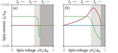
Figure 2: Spin supercurrent $\bm{J}_{\text{s}}$ as a function of spin voltage $V_{\text{s}}$. This spin voltage corresponds to injected (a) spin-$z$ or (b) spin-$x$ accumulation. The light shaded region shows where the system is bistable, and the dark region where superconductivity vanishes.

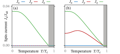
Figure 3: Spin supercurrent $\bm{J}_{\text{s}}$ as a function of temperature $T$ for a fixed spin voltage $eV_{\text{s}}=\Delta_{0}/4$ in the superconductor. This spin voltage corresponds to injected (a) spin-$z$ or (b) spin-$x$ accumulation. The shaded region shows where superconductivity vanishes.

In Fig. 3, we show how the spin supercurrent varies as a function of temperature for a fixed spin voltage $eV_{\text{s}}=\Delta_{0}/4$. Curiously, we find that the spin current increases linearly with decreasing temperature in a relatively large parameter regime. That the spin-$y$ current decreases at the same rate as the spin-$z$ current seems reasonable in light of the equation $\bm{j}_{\text{s}}^{\text{neq}}\sim\bm{j}_{\text{s}}^{\text{eq}}\times\bm{h}_{\text{s}}$: if $\bm{j}_{\text{s}}^{\text{eq}}$ decreases linearly, then $\bm{j}_{\text{s}}^{\text{neq}}$ should do so as well. The most important message from Fig. 3 is perhaps that the nonequilibrium contribution $\bm{j}_{\text{s}}^{\text{neq}}$ to the spin supercurrent remains significant all the way up to the critical temperature of the junction. This means that relevant experiments can be performed at any temperature where superconductivity exists.

Discussion.— In the previous sections, we have shown that injection of a nonequilibrium spin accumulation can be used to generate new spin supercurrent components. The results are especially encouraging since the nonequilibrium contribution to the spin supercurrent can even be made larger than the equilibrium contribution, and we found that it persists all the way up to the critical temperature of the junction. Both these features should make it a particularly interesting effect for experimental detection and future device design. However, there are some questions that we have not addressed yet.

The first question is how the spin source in Fig. 1 works. So far, we have simply treated it as a generic device that manipulates the spin distribution $\bm{h}_{\text{s}}$ inside the superconductor directly. One alternative is to use a normal metal coupled to a voltage-biased ferromagnet [18] or half-metallic ferromagnet [47]. In that case, the polarization of the magnets enable a charge–spin conversion, thus translating an electric voltage into a spin voltage. Another possibility would be spin-pumping experiments, where it is a microwave signal that is translated to a spin voltage [23]. In the limit of weak superconductivity, an expression for the distribution function of a spin-pumped ferromagnet was derived in Ref. [48]. When the precession frequency $\Omega$ and cone angle $\alpha$ are sufficiently small, the result is just a spin voltage $eV_{\text{s}}=\Omega/2$ along the magnetization direction of the ferromagnet. This is the relevant limit for the experiment in Ref. [23]: superconductivity inside Ni₈₀Fe₂₀ is weak, $\Omega\approx 0.5$ meV is much smaller than its magnetic exchange field, and $\alpha\approx 1^{\circ}$ should be small enough to use the leading-order expansions $\sin\alpha\approx\alpha$ and $\cos\alpha\approx 1$.

In all these cases, the spin source necessarily contains magnetic elements, and one challenge would be how to prevent the spin source from affecting the equilibrium spin current. One solution might be to embrace the existing magnets in Fig. 1: one could use the same magnets to generate the equilibrium spin supercurrent and for spin injection. This spin injection may them be performed either using spin pumping—or if the magnets are sufficiently thin for electron tunneling—by placing voltage-biased contacts on top of the magnets. One complication with this strategy is that since the resulting spin accumulation will necessarily be inhomogeneous, both spin supercurrents and resistive spin currents have to coexist.

How to directly measure a spin supercurrent is an open question, although suggestions have recently been proposed [49]. Indirect measurements of spin supercurrents, on the other hand, have already been performed experimentally. Most of these rely on measuring dissipationless charge currents through strongly polarized materials [50; 51; 52; 53; 54; 55; 56; 57]. Since only $\ket{\uparrow\uparrow}$ and $\ket{\downarrow\downarrow}$ pairs can penetrate over longer distances, and the polarization breaks the degeneracy between them, one can infer the existence of spin supercurrents from the measured charge supercurrents.

One solution to the measurement problem might be to look for an inverse effect. We have shown that spin injection into a superconductor results in a torque on the spins transported by the equilibrium spin supercurrent. However, this interaction should cause a reaction torque on the spin source, which might be possible to detect. For instance, in a setup similar to Ref. [18], this reaction torque might directly affect the nonlocal spin conductance. Similarly, in a spin-pumping setup, this might affect the FMR linewidths. In both cases, this reaction torque should only exist when there is an equilibrium spin supercurrent $\bm{j}_{\text{s}}^{\text{eq}}\sim\bm{m}_{{1}}\times\bm{m}_{{2}}$ to interact with, so it should depend on the magnetic configuration of the device.

Conclusion.— We have shown analytically and numerically that if a system harbors a spin supercurrent $\bm{j}_{\text{s}}^{\text{eq}}$ in equilibrium, then a spin injection $\bm{h}_{\text{s}}$ creates a new component $\bm{j}_{\text{s}}^{\text{neq}}\sim\bm{j}_{\text{s}}^{\text{eq}}\times\bm{h}_{\text{s}}$. This effect can be intuitively understood as the injected spins exerting a torque on the spins transported by the equilibrium spin supercurrent, generating a component that is perpendicular to both. These results have implications for the control of spin supercurrents in novel superconducting spintronics devices.

- [1] J. Linder and J. W. A. Robinson, Nat. Phys. 11, 307 (2015).
- [2] M. Eschrig, Physics Today 64, 43 (2010).
- [3] M. Eschrig, Rep. Prog. Phys. 78, 104501 (2015).
- [4] M. G. Blamire and J. W. A. Robinson, J. Phys. Condens. Matter 26, 453201 (2014).
- [5] R. Grein, M. Eschrig, G. Metalidis, and G. Schön, Phys. Rev. Lett. 102, 227005 (2009).
- [6] M. Alidoust, J. Linder, G. Rashedi, T. Yokoyama, and A. Sudbø, Phys. Rev. B 81, 014512 (2010).
- [7] Z. Shomali, M. Zareyan, and W. Belzig, New J. Phys. 13, 083033 (2011).
- [8] P. M. R. Brydon, Y. Asano, and C. Timm, Phys. Rev. B 83, 180504 (2011).
- [9] A. Moor, A. F. Volkov, and K. B. Efetov, Phys. Rev. B 92, 180506 (2015).
- [10] I. Gomperud and J. Linder, Phys. Rev. B 92, 035416 (2015).
- [11] F. Konschelle, I. V. Tokatly, and F. S. Bergeret, Phys. Rev. B 92, 125443 (2015).
- [12] S. H. Jacobsen, I. Kulagina, and J. Linder, Sci. Rep. 6, 23926 (2016).
- [13] X. Montiel and M. Eschrig, Phys. Rev. B 98, 104513 (2018).
- [14] I. V. Bobkova and Y. S. Barash. JETP Lett. 80, 494 (2004).
- [15] J. C. Slonczewski, Phys. Rev. B 39, 6995 (1989).
- [16] D. Beckmann, J. Phys. Condens. Matter 28, 163001 (2016).
- [17] C. H. L. Quay, D. Chevallier, C. Bena, and M. Aprili, Nat. Phys. 9, 84 (2013).
- [18] T. Wakamura, N. Hasegawa, K. Ohnishi, Y. Niimi, and Y. Otani, Phys. Rev. Lett. 112, 036602 (2014).
- [19] F. Hübler, M. J. Wolf, D. Beckmann, and H. v. Löhneysen, Phys. Rev. Lett. 109, 207001 (2012).
- [20] M. Silaev, P. Virtanen, F. S. Bergeret, and T. T. Heikkilä, Phys. Rev. Lett. 114, 167002 (2015).
- [21] I. V. Bobkova and A. M. Bobkov, JETP Lett. 101, 118 (2015).
- [22] I. V. Bobkova and A. M. Bobkov. Phys. Rev. B 93, 024513 (2016).
- [23] K.-R. Jeon, C. Ciccarelli, A. J. Ferguson, H. Kurebayashi, L. F. Cohen, X. Montiel, M. Eschrig, J. W. A. Robinson, and M. G. Blamire, Nat. Mater. 17, 499 (2018).
- [24] T. Taira, M. Ichioka, S. Takei, and H. Adachi. Phys. Rev. B 98, 214437 (2018).
- [25] J. A. Ouassou, T. D. Vethaak, and J. Linder. Phys. Rev. B 98, 144509 (2018).
- [26] F. S. Bergeret, M. Silaev, P. Virtanen, and T. T. Heikkilä. Rev. Mod. Phys. 90, 041001 (2018).
- [27] G. E. W. Bauer, E. Saitoh, and B. J. van Wees, Nat. Mater. 11, 391 (2012).
- [28] V. Chandrasekhar, in Superconductivity (Springer, Berlin, Heidelberg, 2008) pp. 279–313.
- [29] W. Belzig, F. K. Wilhelm, C. Bruder, G. Schön, and A. D. Zaikin, Superlattices and Microstructures 25, 1251 (1999).
- [30] J. Rammer and H. Smith, Rev. Mod. Phys. 58, 323 (1986).
- [31] K. D. Usadel, Phys. Rev. Lett. 25, 507 (1970).
- [32] N. Schopohl, arXiv:cond-mat/9804064.
- [33] S. H. Jacobsen, J. A. Ouassou, and J. Linder, Phys. Rev. B 92, 024510 (2015).
- [34] M. Eschrig, A. Cottet, W. Belzig, and J. Linder, New J. Phys. 17, 083037 (2015).
- [35] P. Machon, M. Eschrig, and W. Belzig, Phys. Rev. Lett. 110, 047002 (2013).
- [36] A. Cottet, D. Huertas-Hernando, W. Belzig, and Y. V. Nazarov, Phys. Rev. B 80, 184511 (2009).
- [37] A. Cottet, Phys. Rev. B 76, 224505 (2007).
- [38] F. Aikebaier, M. A. Silaev, and T. T. Heikkilä, Phys. Rev. B 98, 024516 (2018).
- [39] J. A. Ouassou, S. H. Jacobsen, and J. Linder, Phys. Rev. B 96, 094505 (2017).
- [40] B. S. Chandrasekhar. Appl. Phys. Lett. 1, 7 (1962).
- [41] A. M. Clogston. Phys. Rev. Lett. 9, 266 (1962).
- [42] I. V. Bobkova and A. M. Bobkov, Phys. Rev. B 89, 224501 (2014).
- [43] I. Snyman and Y. V. Nazarov, Phys. Rev. B 79, 014510 (2009).
- [44] J. A. Ouassou and J. Linder, arXiv:1810.02820.
- [45] F. K. Wilhelm, G. Schön, and A. D. Zaikin, Phys. Rev. Lett. 81, 1682 (1998).
- [46] J. J. A. Baselmans, A. F. Morpurgo, B. J. van Wees, and T. M. Klapwijk, Nature 397, 43 (1999).
- [47] I. V. Bobkova and A. M. Bobkov, Phys. Rev. Lett. 108, 197002 (2012).
- [48] M. Houzet. Phys. Rev. Lett. 101, 057009 (2008).
- [49] V. Risinggård and J. Linder. Under preparation (2018).
- [50] R. S. Keizer, S. T. B. Goennenwein, T. M. Klapwijk, G. Miao, G. Xiao, and A. Gupta, Nature 439, 825 (2006).
- [51] M. S. Anwar, F. Czeschka, M. Hesselberth, M. Porcu, and J. Aarts, Phys. Rev. B 82, 100501 (2010).
- [52] J. W. A. Robinson, J. D. S. Witt, and M. G. Blamire, Science 329, 59 (2010a).
- [53] J. W. A. Robinson, G. B. Halász, A. I. Buzdin, and M. G. Blamire, Phys. Rev. Lett. 104, 207001 (2010b).
- [54] T. S. Khaire, M. A. Khasawneh, W. P. Pratt, and N. O. Birge, Phys. Rev. Lett. 104, 137002 (2010).
- [55] J. D. S. Witt, J. W. A. Robinson, and M. G. Blamire, Phys. Rev. B 85, 184526 (2012).
- [56] J. W. A. Robinson, N. Banerjee, and M. G. Blamire, Phys. Rev. B 89, 104505 (2014).
- [57] M. Egilmez, J. W. A. Robinson, J. L. MacManus-Driscoll, L. Chen, H. Wang, and M. G. Blamire, Europhys. Lett. 106, 37003 (2014).