Statistical Treatment of Inverse Problems Constrained by Differential Equations-Based Models with Stochastic Terms

Abstract

This paper introduces a statistical treatment of inverse problems constrained by models with stochastic terms. The solution of the forward problem is given by a distribution represented numerically by an ensemble of simulations. The goal is to formulate the inverse problem, in particular the objective function, to find the closest forward distribution (i.e., the output of the stochastic forward problem) that best explains the distribution of the observations in a certain metric. We use proper scoring rules, a concept employed in statistical forecast verification, namely energy, variogram, and hybrid (i.e., combination of the two) scores. We study the performance of the proposed formulation in the context of two applications: a coefficient field inversion for subsurface flow governed by an elliptic partial differential equation (PDE) with a stochastic source and a parameter inversion for power grid governed by differential-algebraic equations (DAEs). In both cases we show that the variogram and the hybrid scores show better parameter inversion results than does the energy score, whereas the energy score leads to better probabilistic predictions.

LLNL IM Release number: LLNL-JRNL-759502  ANL Preprint # ANL/MCS-P9140-1018

35Q62, 62F15, 35R30, 35Q93, 65C60, 65K10, 62H10, 62M20

1 Introduction

Inverse problems have been traditionally posed as inferring unknown or uncertain parameters (e.g., coefficients, initial conditions, boundary or domain source terms, geometry) that characterize an underlying model from given (possibly noisy) observational or experimental data [59, 26]. Such inverse problems governed by physics-based models, also referred to as data assimilation in the meteorological and climate communities [27], abound in a wider range of application areas such as geophysics, cryosphere studies, medical imaging, biochemistry, and control theory. Typically the models governing these inverse problems are considered deterministic. In reality, however, in addition to the inversion parameter, these models involve other sources of uncertainties and randomness. For instance, the models have multiple uncertain coefficients or unknown or random source terms, parameters that are not—or cannot be—inferred. Motivated by the need to account for these additional uncertainties, researchers in recent years have shown a growing interest in considering inverse problems governed by stochastic (or uncertain) models, mostly in the context of optimal control [62, 10, 46, 34]. In this paper, we consider the inference of parameters for stochastic models (described by differential equations) and quantify the uncertainty associated with this inference.

Contributions

This study introduces a methodology for the statistical treatment of inverse problems constrained by physics-based models with stochastic terms. The salient idea of our approach is to express the problem as finding the inversion parameter for which the stochastic model generates a distribution that best explains the distribution of the observations according to a loss-function we define. To this end, we formulate an

inverse problem with a loss function given by suitable statistical scoring metrics typically employed in forecast verification [55, 20, 19]. Proper scores allow for including in the inversion process a large range of statistical features (e.g., spatial and/or temporal correlations and biases) and, in this respect, are a significant departure from and improvement over the traditional least-squares misfit metrics. We also delve into the issue of how different statistical scores affect the results of the inference problem. This issue becomes important when we explore fitness functions for multivariate distributions because one invariably needs to rely on statistics that typically favor certain features over others, for example, variance over correlations. Traditionally, the solution of the inverse problem is the parameter field (or a distribution if working with statistical inverse problems) that is the closest to the true parameter field in some metric, e.g., least-squares or statistical scores such as those proposed in this work. However, one can also pose the problem as finding the parameter field that generates the most accurate predictions in some statistical sense. In other words, we are interested in how much more predictable the model is after inference/inversion, not necessarily in the goodness of fit. We also explore this alternative inversion paradigm in this study and show that various proper scores or combination of them can be used successfully in different inversion setups (i.e, inverse problems governed by spatial differential equations and time-dependent differential equations) to improve the model predictability.

Another critical issue we address in this paper is the efficient computation of the numerical solution of the proposed statistical inverse problems. Namely, we propose a solution approach based on numerical optimization and provide the ingredients, in the form of gradient-based scalable optimization algorithms and adjoint sensitivities, that are needed to ensure the scalability of our methodology to large-scale problems. More specifically, to compute the most fit parameter field, we solve an optimization problem (implicitly) constrained by the stochastic model with a quasi-Newton limited-memory secant algorithm, BFGS updates for the inverse of the Hessian of the cost function, and an Armijo line search. If the objective function is a likelihood function and if prior information is available, then this approach is equivalent to computing the maximum likelihood or maximum a posteriori (MAP) point.

We derive adjoint-based expressions for efficient computation of the gradient of the objective with respect to the inversion parameters. We illustrate our approach with two problems. The first is an inversion for the coefficient field in an elliptic partial differential equation (PDE), interpreted as a subsurface flow problem under a stochastic source field. The second problem is represented by the inversion for a parameter in a differential-algebraic system of equations (DAEs) under stochastic load terms. This model can represent a power grid system with uncertain load behavior, which induces small transients in the system, the goal here being to determine the dynamic parameters within a quasi-stationary regime.

Problem formulation

In what follows, let us consider that we have a mathematical model expressed as $F(u,m;\xi)=0$, with states $u$ and parameters $m$ driven by a stochastic forcing $\xi$ with known probability law. Formally, such a model can consist of a standard stochastic PDE on a domain $\mathcal{D}\subset\mathbb{R}^{d}$ ($d=1,2,3$) with suitable boundary $\Gamma$; in this case $u$ is a function on $\mathcal{D}$ and $\xi:\Omega\rightarrow\mathbb{R}^{p}$ ($p=2,3$) is defined by means of a probability space $(\Omega,\mathcal{F},\mathbbm{P})$, where $\Omega$ is the sample space (the set of all possible events), $\mathcal{F}$ is the $\sigma-$algebra of events, and $\mathbbm{P}:\mathcal{F}\rightarrow[0,1]$ is a probability measure. We assume that this probability space is completely defined. We take $m$ to be a real-valued deterministic field, although extensions to random fields are also possible. Formally, the mathematical model can be defined as in [23] in the following form:

(1) $$F(u(\cdot,\xi),m(\cdot,\xi);\xi(\cdot))=0~{}\textnormal{a.s.}\,,~{}\textnormal{with}~{}F\in\mathcal{D}~{}\textnormal{a.e.},\,u\in\overline{\mathcal{D}}\times\Omega\rightarrow\mathbb{R},\,m\in\mathbb{R}^{d},\,\xi\in\mathbb{R}^{p}\,.$$

We also assume that we have a suitable vector space with finite stochastic moments when $F$ is a PDE. More details on the setup can be found in [22]. In this work $F$ is defined by a PDE (see Sec. 4) or an ordinary differential equation (ODE)/DAE (see Sec. 5) system. We assume the availability of sparse observations ${\boldsymbol{d}_{\scriptscriptstyle\text{obs}}}$ of the states $u$ corresponding to the true parameters, which we denote by $m_{\scriptscriptstyle\text{true}}$.

At the high level, the inverse problem formulation we use in this work is standard: Given model (1) and observations ${\boldsymbol{d}_{\scriptscriptstyle\text{obs}}}=\mathcal{F}(m_{\scriptscriptstyle\text{true}})+\varepsilon_{\rm obs}$ such that $F(u,m_{\scriptscriptstyle\text{true}};\xi)=0$ a.s., find $m$ that generates model predictions that best explain the observations under a certain metric. The function $\mathcal{F}(m_{\scriptscriptstyle\text{true}})$ is the so-called parameter-to-observable map whose evaluation involves the solution of the given ODE/PDE followed by the application of an observation operator $\mathcal{B}$, i.e., $\mathcal{F}(m_{\scriptscriptstyle\text{true}})=\mathcal{B}u(m)$, where $u$ solves $F(u,m_{\scriptscriptstyle\text{true}};\xi)=0$. The observations are subject to known observational noise $\varepsilon_{\rm obs}$, which we assume to be a random vector with known Borel probability measure $\pi_{\mbox{\tiny obs}}$, in addition to and independent of the stochastic forcing $\xi$. A commonly used metric is the distance between the observables predicted by the model $\mathcal{F}(m)$ and the actual observations ${\boldsymbol{d}_{\scriptscriptstyle\text{obs}}}$. The metrics used in this work are referred to as statistical score functions that compute the fitness or a distance between the distribution of the observables $\mathcal{F}(m)$ and the set of validation data, namely, observations ${\boldsymbol{d}_{\scriptscriptstyle\text{obs}}}$. We denote these score functions by $S(\mathcal{F}(m),{\boldsymbol{d}_{\scriptscriptstyle\text{obs}}})$, where $\mathcal{F}(m)$ and ${\boldsymbol{d}_{\scriptscriptstyle\text{obs}}}$ represent the model predictions and the observations, respectively. We introduce and discuss in detail such score functions in the next section.

Scores are positive functions that achieve their global minimum when observations and model predictions are statistically indistinguishable. For that reason scores have been used as loss or utility functions in order to assess the level of confidence one has in the probabilistic model prediction [28, 18]. Therein, the maximum score estimation is introduced as a generalization of maximum likelihood estimation. A likelihood function can be defined as $\pi_{\mbox{\tiny like}}({\boldsymbol{d}_{\scriptscriptstyle\text{obs}}}|m)\propto\exp\left(-S(\mathcal{F}(m),{\boldsymbol{d}_{\scriptscriptstyle\text{obs}}})\right)$ as a measure describing the relative plausibility of the parameter value [42]. Therefore, the inverse problem can be formulated as finding $m^{*}$ such that

(2) $$m^{*}=\arg\min_{m}\mathcal{J}(m)~{}\textnormal{ subject to }~{}F(u,m;\xi)=0\,\textnormal{ a.s. }$$

where $\xi$ is known, and where, for instance, $\mathcal{J}(m)=-\log(\pi_{\mbox{\tiny like}}({\boldsymbol{d}_{\scriptscriptstyle\text{obs}}}|m))$. In practice, we assume that we have access to a vector of $M$ observations ${\boldsymbol{d}_{\scriptscriptstyle\text{obs}}}\in\mathbb{R}^{M}$ and can generate an ensemble of ${N_{s}}$ model predictions $\mathcal{F}(m)\in\mathbb{R}^{M\cdot{N_{s}}}$.

The objective in (2) depends on the observed data ${\boldsymbol{d}_{\scriptscriptstyle\text{obs}}}$ via a single or multiple realizations, the numerical model observables output $\mathcal{F}(m)$, and potentially explicitly on the parameter $m$. In this study we will follow the inverse Bayesian nomenclature with $m^{*}$ being the MAP point. We remark that the optimization problem also depends on the parameter $m$ implicitly through the PDE or ODE/DAE constraint described by $F$.

Related work

Inverse problems with stochastic parameters are typically addressed in a multilevel context. Here the stochasticity may come from reducing the models and introducing a stochastic term that accounts for the model reduction error [3, 30]. In other cases, the additional stochastic/uncertain input is treated as a nuisance parameter and an approximate premarginalization over this parameter is carried out [36, 26, 25]. In this study we consider the case when stochasticity is inherent in the problem and we do not have access to a deterministic version of a complete model. In the optimal control community, recent efforts have targeted moment matching between a stochastic controlled PDE and observations, [62, 10, 46]. In most cases the loss function is based on statistics of univariate or marginal distributions. Various classical data discrepancy functions (utility/loss) for inverse problems including Kullback-Leibler divergence are discussed [60]. Extending to multivariate settings is extremely challenging because of the difficulty of accounting for complex dependencies, the curse of dimensionality, and the lack of order or rank statistics.

The scoring functions used in this study are precisely addressing the multivariate aspect of the model and observational data distributions. A strategy similar to what we present here has been introduced in the statistical community sometimes under the name of statistical postprocessing or model output statistics. It consists of altering the computational model probabilistic forecasts by postprocessing the ensemble forecasts, and it tends to address the issue of bias and dispersion [19]. Most of these approaches are variations of Bayesian model averaging discussed in [45] and the nonhomogeneous regression model proposed in [19]. In these strategies the numerical model or its parameters are not controlled; only its output is adjusted [52, 29, 6, 7, 50, 55, 15]. In the strategy proposed in this study, the model itself through its parameters is part of the control space. Therefore, our approach then can be interpreted as calibrating a generative model [8] or model generator [51, 32], where parameter $m$ modulates the distribution of a physical model simulator. In this context there are several strategies that aim to minimize a certain distance between the generator and the truth. The distance can be minimized between various statistics of the generator outputs and the true data such as cumulative distribution function, density, or moments. Those methods pertain to the class of minimum distance estimation in which usual metric distances have been used such as the Chi-square, the least-squares, or Kolmogorov-Smirnov. However, with increasingly complex models and complex distributions, exact derivations of cost-functions becomes intractable and approximation of distributions are obtained through strategies such as Approximate Bayesian computations [33]. Many of these methods are emergent in the variational inference and machine learning communities [63], where the Kullback-Leibler divergence tends to be the most popular combined with sampling algorithms. In the proposed work we propose use multivariate scoring metrics used in statistical forecast evaluation field, which provide a computational attractive, flexible, and extensible alternative to existing metrics.

The remaining sections of this paper are organized as follows. We begin by introducing the scoring functions and discuss the property needed in order for the ansatz (2) to be well posed in Section 2. In Sections 4 and 5 we introduce a prototype elliptic PDE-based model problem with application in subsurface flow and a time-dependent problem driven by DAEs with application in power grid modeling, respectively. We conclude in Section 6 with a discussion of the method, results, and its limitations.

2 Scoring and metrics

In statistics one way to quantitatively compare or rank probabilistic models is using score functions. A score function is a scalar metric $S$ that takes as inputs (i) verification data, in our inverse problem formulation the observations ${\boldsymbol{d}_{\scriptscriptstyle\text{obs}}}$, and (ii) outputs from the model to be evaluated, those outputs can be quantities describing the model (for instance parameters of probabilistic distribution) or model outputs, in the present work are the observables subject to observational noise, namely, $\mathcal{F}(m)$, independent of the stochastic forcing $\xi$, and returns a scalar used to scoring or ranking verification outputs with respect to the verification data. These scores are commonly used in forecast evaluation where competing forecasts are compared [54]. Scores are generally used in a negatively-oriented fashion, the smaller the score, the closer to the verification data is the model at stake.

While evaluating numerical model simulations, one aims to detect bias, trends, outliers, or correlation misspecification. To create an objective function that can distinguish among different modeling strategies, one needs appropriate mathematical scoring metrics to rank them. Complex mathematical properties are required for consistent ranking of the models [18].

Score functions use different statistics to distinguish among different (statistical) models. Moreover, in order to be able to distinguish among and consistently rank different models, score functions are required to have specific mathematical properties. Proper score functions are widely used in statistics to ensure consistent ranking, for example in forecast evaluation, where competing forecasts are compared [54]. The following definition of proper scoring is from [18].

Definition 2.1.

For the considered probability space $(\Omega,\mathcal{F},\mathbbm{P})$, a score $S:\mathcal{P}\times\Omega\rightarrow\mathbb{R}$ is proper relatively to the class of probability measure $\mathcal{P}$ iff

(3) $$\mathbb{E}_{Y}\{S(P_{Y},Y)\}\leq\mathbb{E}_{Y}\{S(P,Y)\}\,,\forall P\in\mathcal{P}\,,$$

where $\mathcal{P}$ is a convex class of probability measures on $(\Omega,\mathcal{F})$, and $P_{Y}$ is the probability distribution of $Y$.

In other words, this definition states that a proper scoring rule prevents a score from favoring any probabilistic distribution over the distribution of the verification data. In addition, a proper score has two main desired features: (1) statistical consistency between the verification data and the model outputs, called calibration, and (2) reasonable dispersion in the model outputs, provided they are calibrated, which is referred to as sharpness. In statistics, the trend is to build proper scores that access simultaneous calibration and sharpness.

Various functions can be used to assess the error between the verification data and model outputs; however, scoring is not restricted to pointwise comparison. Methods to evaluate the quality of unidimensional outputs are well understood [17]; however, the evaluation of multidimensional outputs or ensemble of outputs has been addressed in the literature more recently [20, 43, 49] and remains challenging. The energy and variogram-based scores (detailed below) are well suited to multiple multidimensional realizations of a same model to be verified. Therefore, in this paper we will focus on these scores and combination of them.

A widely accepted score is the continuous ranked probability score (CRPS):

(4) $$S_{\textnormal{CRPS}}(P,y)=\int_{-\infty}^{\infty}\left(F_{X}(x)-\mathbbm{1}_{x<y}\right)^{2}\mathrm{d}x\,,\quad\,$$

where $F_{X}$ is the cumulative distribution function (CDF) of $X\sim P$, $F_{X}(x)=\mathbbm{P}[X\leq x]$, and $\mathbbm{1}_{x<y}$ is the Heavyside function. The CRPS computes a distance between a full probability distribution and a single deterministic observation, where both are represented by their CDF. However, this score is only univariate and cannot be used if the dimension of the observations is larger than one. In the following, we consider the energy score and the variogram-based score that are both scores expressed in a multi-dimensional context.

Moreover, closed forms of the scores are not always computable, consequently one uses Monte Carlo approximation of the scores by deriving them with samples from the predictive distribution of interest. For this reason, the energy and variogram-based scores will be computed using ${N_{s}}$ samples in the following. Approximated scores can then be expressed with discrete arguments as $S:\mathbb{R}^{M\cdot{N_{s}}}\times\mathbb{R}^{M}\rightarrow\mathbb{R}$, which is applied to $\mathcal{F}(m)$, which is represented by ${N_{s}}$ model prediction samples of dimension $M$ and an observation or validation vector, ${\boldsymbol{d}_{\scriptscriptstyle\text{obs}}}$, of size $M$.

2.1 Energy score

The energy score [20] is multivariate and proper. It generalizes CRPS (4) from univariate to multivariate and can be expressed as

(5) $$S({\boldsymbol{d}},{\boldsymbol{d}_{\scriptscriptstyle\text{obs}}}) =\mathbb{E}_{P}\|{\boldsymbol{d}}^{a}-{\boldsymbol{d}_{\scriptscriptstyle\text{obs}}}\|-\frac{1}{2}\mathbb{E}_{P}\|{\boldsymbol{d}}^{a}-{\boldsymbol{d}}^{b}\|\,,~{}{\boldsymbol{d}_{\scriptscriptstyle\text{obs}}}\sim P_{T}\,,~{}\forall{\boldsymbol{d}}^{a},{\boldsymbol{d}}^{b}\sim P\,,$$

where, in the context of this study, ${\boldsymbol{d}}=\mathcal{F}(m)$ which is considered a realization of probability distribution. This score is sensitive to bias and variance discrepancy, but potentially less sensitive to correlations; it will be denoted as the ES-model.

In the probabilistic forecast context, scores can be used as a loss function to fit probabilistic predictive distributions to observations; for instance, see [48]. Similarly to this idea, we propose to use statistical proper scores as objective functions in the underlying inverse problems. In this context, the score $S$ could, for instance, be the energy score; and if only samples from distribution $P$ are available, it can be defined as follows:

(6) $$S_{\mathrm{ES}}:=S({\boldsymbol{d}},{\boldsymbol{d}_{\scriptscriptstyle\text{obs}}})=\frac{1}{{N_{s}}}\sum_{i=1}^{{N_{s}}}||{\boldsymbol{d}}^{(i)}-{\boldsymbol{d}_{\scriptscriptstyle\text{obs}}}||-\frac{1}{2{N_{s}}^{2}}\sum_{i=1}^{{N_{s}}}\sum_{j=1}^{{N_{s}}}||{\boldsymbol{d}}^{(i)}-{\boldsymbol{d}}^{(j)}||,$$

where ${N_{s}}$ is the number of model prediction samples and ${\boldsymbol{d}}^{(i)}=\{\mathcal{F}(m)\}^{(i)}=\mathcal{B}u^{(i)}(m)$ are model predictions corresponding to $i$th sample of the stochastic model forcing, $\xi^{(i)}$, evaluated at parameter $m$. Here $\mathcal{B}$ is a linear observation operator that extracts measurements from $u$.

2.2 Variogram score

The variogram-based score [49] is multivariate, proper, more sensitive to covariance (structure) but insensitive to bias. Its approximated sample version is given by

(7) $$S_{\mathrm{VS}}:=S({\boldsymbol{d}},{\boldsymbol{d}_{\scriptscriptstyle\text{obs}}})=\sum_{i=1}^{M}\sum_{j=1}^{M}w_{ij}\left(|{\boldsymbol{d}_{\scriptscriptstyle\text{obs}}}(i)-{\boldsymbol{d}_{\scriptscriptstyle\text{obs}}}(j)|^{p}-\frac{1}{{N_{s}}}\sum_{k=1}^{{N_{s}}}|{\boldsymbol{d}}^{(k)}(i)-{\boldsymbol{d}}^{(k)}(j)|^{p}\right)^{2}\,,~{}p>0\,,$$

where we take $p=2$, $M$ is the dimension of observations ${\boldsymbol{d}_{\scriptscriptstyle\text{obs}}}$ (e.g., number of observational points in space), and $w_{ij}$ is a function of the distance of the position of observation $i$ and observation $j$. In other words we take differences between every observation and then of the corresponding expectation of the scenarios. If we denote $\boldsymbol{\delta}_{ij}=\boldsymbol{e}_{i}-\boldsymbol{e}_{j}$, where $\boldsymbol{e}_{i}$ is the unit vector with the $i^{th}$ component $1$, the preceding equation becomes

(8) $$S({\boldsymbol{d}},{\boldsymbol{d}_{\scriptscriptstyle\text{obs}}})=\sum_{i=1}^{M}\sum_{j=1}^{M}w_{ij}\left(|\boldsymbol{\delta}^{T}_{ij}\;{\boldsymbol{d}_{\scriptscriptstyle\text{obs}}}|^{p}-\frac{1}{{N_{s}}}\sum_{k=1}^{{N_{s}}}|\boldsymbol{\delta}^{T}_{ij}\;\mathcal{B}u^{(k)}|^{p}\right)^{2}.$$

This will be referred to as the VS-model.

2.3 Discussion and other scores

The energy score is known for failing to discriminate misspecified correlation structures of the fields, but it successfully identifies fields with expectation similar to the one of the verifying data. On the other hand, the variogram-based score fails to discriminate fields with misspecified intensity, but it discriminates between correlation structures [44, 49]. Because of these different features and in order to discriminate fields according to their intensity and correlation structure, we propose to use a linear combination of the two scores, namely,

(9) $$S_{\mathrm{HS}}({\boldsymbol{d}},{\boldsymbol{d}_{\scriptscriptstyle\text{obs}}})= \alpha S_{\mathrm{ES}}({\boldsymbol{d}},{\boldsymbol{d}_{\scriptscriptstyle\text{obs}}})+\beta S_{\mathrm{VS}}({\boldsymbol{d}},{\boldsymbol{d}_{\scriptscriptstyle\text{obs}}})\,,$$

where $\alpha>0$ and $\beta>0$ are problem specific. We will refer to this hybrid score as the HS-model. It is also a proper score because any linear positive combination of proper scores remains a proper score.

The score functions defined above are referred to as instantaneous scores because they are functions of one verification data-point (${\boldsymbol{d}_{\scriptscriptstyle\text{obs}}}\in\mathbb{R}^{M}$). If more than one verification sample is available—for example, if we have $n$ samples of ${\boldsymbol{d}_{\scriptscriptstyle\text{obs}}}^{(1,\dots,n)}=[{\boldsymbol{d}_{\scriptscriptstyle\text{obs}}}^{(1)},{\boldsymbol{d}_{\scriptscriptstyle\text{obs}}}^{(2)},\dots\boldsymbol{d}_{\scriptscriptstyle\text{obs}}^{(n)}]^{\top}\in\mathbb{R}^{n\times M}$ from the true distribution—then we can estimate the mean score defined as follows:

(10) $$S_{n}({\boldsymbol{d}},{\boldsymbol{d}_{\scriptscriptstyle\text{obs}}}^{(1,\dots,n)})=\frac{1}{n}\sum_{i=1}^{n}S({\boldsymbol{d}},{\boldsymbol{d}_{\scriptscriptstyle\text{obs}}}^{(i)})\,.$$

In most cases, scores are used on verification data that are assumed to be perfect. In practice, however, observations are almost always tainted with errors. Limited recent studies on forecast verification attempt to address this issue [14, 35]. Incorporating error and uncertainty in the scoring setup is challenging. Analytical results are tractable only in particular cases such as linear or multiplicative noise with Gaussian and Gamma distributions, respectively. One way of tackling the observational error is to assume some probability distributions for the observations and the model outputs and to consider a new score defined as the conditional expectation of the original score given the observations [35]. Using the notations of Definition 2.1, we can express the corrected score as $S_{corr}(P,y)=\mathbb{E}(S(P,X)|Y=y)$, where $X$ represents the hidden true state of the system. In practice, to implement this method, one has to assume some distribution for the $X$ and $Y$ and access an estimation of the distribution parameters. If the errors are i.i.d., then their contribution can be factored out when using the score as a loss function. This is the case under consideration in this study.

Statistical properties of scores

Approximated scores are asymptotically unbiased and consistent (convergent in probability) by the virtue of the Law of Large Numbers. Moreover, as discussed in the introduction, scores can be used as loss functions, this procedure falls into the class of optimum contrast estimation. Asymptotical results about their consistency of optimum contrast estimators can be found in [42]. Strictly proper scoring rules as a contrast function is discussed in [18]. In the case of non-strictly propriety, which is also the case in our study, one may loose the uniqueness of the limit point. Namely, under regularity assumptions, the optimum estimator would converge to a point that belongs to a set of optima of the proper score. Multivariate strictly proper scores for non-standard distributions are typically intractable, and hence, in this study we focus on proper scores, which are practical. Moreover, proper scores can be seen as divergence functions; however, they typically do not satisfy the triangular inequality. We will refer in text to distance or metric in this weaker sense.

3 Model problems

To probe the proposed statistical treatment of inverse problems constrained by differential equations-based models with stochastic inputs, we consider two model problems. The first is a coefficient field inversion for subsurface flow governed by an elliptic PDE with a stochastic input, in other words, a PDE-constrained model problem (Section 4); the second is a parameter identification problem for power grid governed by DAEs with stochastic input, in other words, a DAE-constrained model problem (Section 5). For both problems, we generate synthetic observations ${\boldsymbol{d}_{\scriptscriptstyle\text{obs}}}$ by using one or more samples $\xi^{(i)}\sim\pi_{\mbox{\tiny$\xi$}}$, $i=1,\dots,{N_{s}}$; where $\pi_{\mbox{\tiny$\xi$}}$ is a known distribution. These samples then enter into the forward models with a parameter considered the truth, $m_{\scriptscriptstyle\text{true}}$. We then solve the optimization problem (2) to obtain the maximum utility or the maximum likelihood by evaluating the likelihood function $\mathcal{J}(m)=S(\mathcal{F}(m),{\boldsymbol{d}_{\scriptscriptstyle\text{obs}}})$ and for the MAP point by maximizing the a posteriori probability density function $\mathcal{J}(m)=S(\mathcal{F}(m),{\boldsymbol{d}_{\scriptscriptstyle\text{obs}}})+\mathcal{R}(m)$ with the precomputed ${N_{s}}$ scenarios $\xi^{(i)}$ such that $F(u^{(i)},m;\xi^{(i)})=0$, $i=1,\dots,{N_{s}}$. To solve the PDE-constrained model problem efficiently, in Section 4.1 we derive the gradient of the objective function $\nabla_{m}\mathcal{J}(m)$ with respect to these fixed scenarios using adjoints. We remark that our calculations use classical Monte Carlo to estimate the solution of the problem at hand; however, more sophisticated methods such as higher-order [21] or multilevel [16] Monte Carlo methods can be used to solve the underlying stochastic PDE.

4 Model problem 1: Coefficient field inversion in an elliptic PDE with a random input

In this section, we study the inference of the log coefficient field in an elliptic partial differential equation with a random/stochastic input. This example can model, for instance, the steady-state equivalent for groundwater flows [34]. For simplicity, we state the equations using a deterministic right-hand side. We will then turn our attention to the case where the volume source terms are stochastic. To this end, consider the forward model

(11) $$\begin{split}-\nabla\cdot(e^{{m}}\nabla u)&=f\quad\text{ in }\mathcal{D},\\ u&=g\quad\text{ on }\Gamma_{\!\!D},\\ e^{{m}}\nabla{u}\cdot\boldsymbol{n}&=h\quad\text{ on }\Gamma_{\!\!N},\end{split}$$

where $\mathcal{D}\subset\mathbb{R}^{d}$ ($d=2,3$) is an open bounded domain with sufficiently smooth boundary $\Gamma=\Gamma_{\!\!D}\cup\Gamma_{\!\!N}$, $\Gamma_{\!\!D}\cap\Gamma_{\!\!N}=\emptyset$. Here, $u$ is the state variable; $f\in L^{2}(\mathcal{D})$, $g\in H^{1/2}(\Gamma_{\!\!D})$, and $h\in L^{2}(\Gamma_{\!\!N})$ are volume, Dirichlet, and Neumann boundary source terms, respectively; and $m$ is an uncertain parameter field in $\mathcal{E}=\mathsf{dom}(\mathcal{A})$, where $\mathcal{A}$ is a Laplacian-like operator, as defined in  [53, 1] and for completeness repeated in Section 4.3. To state the weak form of (11), we define the spaces,

$$\mathscr{V}_{\!g}=\{v\in H^{1}(\mathcal{D}):{\left.\kern-1.2pt{v}\vphantom{\big{|}}\right|_{\Gamma_{\!\!D}}}=g\},\quad\mathscr{V}_{\!\scriptscriptstyle{0}}=\{v\in H^{1}(\mathcal{D}):{\left.\kern-1.2pt{v}\vphantom{\big{|}}\right|_{\Gamma_{\!\!D}}}=0\},$$

where $H^{1}(\mathcal{D})$ is the Sobolev space of functions in $L^{2}(\mathcal{D})$ with square integrable derivatives. Then, the weak form of (11) is as follows: Find $u\in\mathscr{V}_{\!g}$ such that

$${\left\langle{e^{{m}}\nabla{u}},{\nabla{p}}\right\rangle}={\left\langle{f},{p}\right\rangle}+{\left\langle{h},{p}\right\rangle}_{\Gamma_{\!\!N}},\quad\forall p\in\mathscr{V}_{\!\scriptscriptstyle{0}}.$$

Here ${\left\langle{\cdot},{\cdot}\right\rangle}$ and ${\left\langle{\cdot},{\cdot}\right\rangle}_{\Gamma_{\!\!N}}$ denote the standard inner products in $L^{2}(\mathcal{D})$ and $L^{2}(\Gamma_{\!\!N})$, respectively.

In what follows we treat $f$ as a stochastic term, denoted by $\xi$ for consistency, given by a two-dimensional heterogeneous Gaussian process with known distribution $\pi_{\mbox{\tiny$\xi$}}$. We use the instantaneous scores defined in Section 2 for this model.

4.1 Adjoint and gradient derivation

We apply an adjoint-based approach to derive gradient information with respect to the parameter field $m$ for the optimization problem (2) with $\mathcal{J}(m)=S(\mathcal{F}(m),{\boldsymbol{d}_{\scriptscriptstyle\text{obs}}})+\mathcal{R}(m)$, namely

(12) $$\min_{m\in\mathcal{E}}S(\mathcal{F}(m),{\boldsymbol{d}_{\scriptscriptstyle\text{obs}}})+\mathcal{R}(m)\,,$$

where $\mathcal{F}(m)$ corresponds to solving the forward problem (11) ${N_{s}}$ times, and $\mathcal{R}(m)$, which will be explicitly defined in the Computational experiment Section 4.3, is a regularization/prior term.

The adjoint equations are derived through a Lagrangian formalism [56]. To this end, the Lagrangian functional can be written as

(13) $$\mathscr{L}(u,m,p):=S(\mathcal{F}(m),{\boldsymbol{d}_{\scriptscriptstyle\text{obs}}})+\mathcal{R}(m)+\sum_{i=1}^{{{N_{s}}}}\biggl{[}{\left\langle{e^{{m}}\nabla u^{(i)}},{\nabla p^{(i)}}\right\rangle}-{\left\langle{\xi^{(i)}},{p^{(i)}}\right\rangle}-{\left\langle{p^{(i)}},{h}\right\rangle}_{\Gamma_{\!\!N}}\biggr{]},$$

where $p^{(i)}\in\mathscr{V}_{\!\scriptscriptstyle{0}}$ is the adjoint corresponding to state $u^{(i)}\in\mathscr{V}_{\!g}$. The formal Lagrangian formalism yields that, at a minimizer of (2), variations of the Lagrangian functional with respect to all variables vanish. Thus we have

(14a) $${\left\langle{e^{{m}}\nabla u^{(i)}},{\nabla\tilde{p}}\right\rangle}-{\left\langle{\xi^{(i)}},{\tilde{p}}\right\rangle}-{\left\langle{\tilde{p}},{h}\right\rangle}_{\Gamma_{\!\!N}} =0,$$

(14b) $${\left\langle{e^{{m}}\nabla\tilde{u}},{\nabla p^{(i)}}\right\rangle}+{\left\langle{r^{(i)}},{\tilde{u}}\right\rangle} =0,$$

(14c) $$\sum_{i=1}^{{N_{s}}}{\left\langle{\tilde{m}e^{{m}}\nabla u^{(i)}},{\nabla p^{(i)}}\right\rangle} =0,$$

for all variations $(\tilde{u},\tilde{m},\tilde{p})\in\mathscr{V}_{\!\scriptscriptstyle{0}}\times\mathcal{E}\times\mathscr{V}_{\!\scriptscriptstyle{0}}$ and $i=1,\ldots,N_{s}$. Note that (14a) and (14b) are the weak forms of the state and of the adjoint equations, respectively. The adjoint right-hand side $r^{(i)}$ in strong form for the energy score (6) is

(15) $$r^{(i)}=\frac{1}{2{N_{s}}}\frac{\mathcal{B}^{*}(\mathcal{B}u^{(i)}-{\boldsymbol{d}_{\scriptscriptstyle\text{obs}}})}{||\mathcal{B}u^{(i)}-{\boldsymbol{d}_{\scriptscriptstyle\text{obs}}}||}-\frac{1}{{N_{s}}^{2}}\sum_{j=1}^{{N_{s}}}\frac{\mathcal{B}^{*}(\mathcal{B}u^{(i)}-\mathcal{B}u^{(j)})}{||\mathcal{B}u^{(i)}-\mathcal{B}u^{(j)}||},$$

and for the variogram score (7) the $h^{th}$ component of $r^{(i)}$ is

(16) $$r_{h}^{(i)}=-\frac{4}{{N_{s}}}\sum_{l=1}^{M}w_{lh}\mathcal{C}(u_{h}^{(i)},u_{l}^{(i)})\;\mathcal{B}^{*}\boldsymbol{\delta_{lh}}\;\boldsymbol{\delta^{T}_{lh}}\;\mathcal{B}u^{(i)},$$

for $i=1,\dots,{N_{s}}$, and for $h=1,\dots,M$. Here

(17) $$\mathcal{C}(u_{h}^{(i)},u_{l}^{(i)}) =|{\boldsymbol{d}_{\scriptscriptstyle\text{obs}}}(h)-{\boldsymbol{d}_{\scriptscriptstyle\text{obs}}}(l)|^{2}-\frac{1}{{N_{s}}}\sum_{k=1}^{{N_{s}}}|\underset{\mathcal{B}u^{(k)}(h)}{\underbrace{\{\mathcal{F}(m)\}^{(k)}(h)}}-\underset{\mathcal{B}u^{(k)}(l)}{\underbrace{\{\mathcal{F}(m)\}^{(k)}(l)}}|^{2}$$

$$=|\boldsymbol{\delta}^{T}_{hl}\;{\boldsymbol{d}_{\scriptscriptstyle\text{obs}}}|^{2}-\frac{1}{{N_{s}}}\sum_{k=1}^{{N_{s}}}|\boldsymbol{\delta}^{T}_{hl}\;\mathcal{B}u^{(k)}|^{2},$$

where $\mathcal{B}u^{(k)}(l)$ denotes the $l^{th}$ component of $\mathcal{B}u^{(k)}$, namely, $\sum_{j=1}^{M}\mathcal{B}_{jl}u_{j}^{(k)}$.

The left-hand side in (14c) gives the gradient for the cost functional (2), which is the Fréchet derivative of $S(\mathcal{F}(m),{\boldsymbol{d}_{\scriptscriptstyle\text{obs}}})$ with respect to $m$. In strong form this is

(18) $$\mathcal{G}(m)=\sum_{i=1}^{{N_{s}}}{\left\langle{e^{{m}}\nabla u^{(i)}},{\nabla p^{(i)}}\right\rangle}+\mathcal{R}_{m}(m),$$

where $u^{(i)}$ and $p^{(i)}$ are solutions to the $i^{th}$ state and adjoint equations, respectively, and $\mathcal{R}_{m}(m)$ is the derivative of the regularization/prior term with respect to the parameter $m$ [56, 9]. The scaling of the regularization term is problem specific and should be addressed case-by-case.

We would like to add the following remarks about the adjoint problem: (1) it is driven only by the derivative of the scoring functions with respect to the forward solution; and (2) the forward and adjoint problems share the same PDE operator, therefore the same solution method can be applied to solve these PDEs. Computing the gradient information via adjoints for large-scale PDE-constrained optimization problems is imperative. Via an adjoint approach, the cost of the gradient evaluation is one forward and one adjoint PDE solve per optimization iteration [41].

4.2 Computational approach and cost

The inverse problems (2) are solved by using hIPPYlib (an inverse problem Python library [58, 57]). It implements state-of-the-art scalable adjoint-based algorithms for PDE-based deterministic and Bayesian inverse problems. It builds on FEniCS [13, 31] for the discretization of the PDEs and on PETSc [4, 5] for scalable and efficient linear algebra operations and solvers needed for the solution of the PDEs.

The gradient computation technique presented in the preceding section allows using state-of-the-art nonintrusive computational techniques of nonlinear programming to solve the estimation problems (2) efficiently for the energy and variogram scores we propose, as well as any combination of them. More specifically, we use a quasi-Newton limited-memory secant algorithm with BFGS updates for the inverse of the Hessian [37, 9] and an Armijo line search  [37] to solve (2) as an unconstrained optimization problem. This quasi-Newton solution approach is appealing since it can have fast local convergence properties similar to Newton-like methods without requiring Hessian evaluations and it also converges from remote starting points as robust as a gradient-based algorithm. In our computations the total number of quasi-Newton iterations was reasonably low, varying between $60$ and $160$. The implementation in hIPPYlib uses an efficient compact limited-memory representation [12] of the inverse Hessian approximation that has reduced space and time computational complexities, namely, $O(|m|\times l)$, where $|m|$ denotes the cardinal of the discretization vector of $m$ and $l$ is the length of the quasi-Newton secant memory (usually taken as $O(10))$.

The computational cost per iteration is overwhelmingly incurred in the evaluation of the objective function in (2) and its gradient. For both the energy and variogram scores, the evaluation of the objective and its gradient requires $N_{s}$ forward PDE solves and adjoint PDE solves, respectively, to compute states $u^{(i)}$ in (14a) and adjoint variables $p^{(i)}$ in (14b). To achieve this, the projected states $d^{(i)}$ appearing in (6) and (15) are stored in memory to avoid the expensive re-evaluations of the PDEs and state projections for the computation of the score $S$ in (6) and adjoint right-hand side in (15). Similarly, for the variogram score, in the evaluation of the objective function we save the terms $\mathcal{C}(u_{h}^{(i)},u_{l}^{(i)})$ ($h,l=1,\ldots,M$) as a $M\times M$ matrix for each $i=1,\ldots,N_{s}$ and reuse them in the computation of the adjoint right-hand sides (16) during the objective gradient evaluation. This approach effectively avoids $N_{s}$ expensive re-evaluations of the PDEs at the cost of $O(N_{s}M^{2})$ extra storage.

From (6) and (15) one can see that the computation of the energy score and its gradient also includes a $O(N_{s}^{2}\cdot M)$ complexity term in addition to the forward and adjoint solves. A similar extra complexity term is present in the computation of the variogram score from (7) and its adjoint right-hand size from (16).

Undoubtedly, the objective and gradient computations can be parallelized efficiently for both scores because of the presence of the summation operators. In particular, both scores allow a straightforward scenario-based decomposition that allows the PDE (forward and adjoint) solves to be done in parallel. Coupled with the (lower-level) parallelism achievable in hIPPYlib via DOLFIN and PETSc, this approach would result in an effective multilevel decomposition with potential for massive parallelism and would allow tackling complex PDEs and a large number of scenarios. The quasi-Newton method based on secant updates used in this work can be parallelized efficiently, as one of the authors has shown recently [38].

We remark that a couple of potential nontrivial parallelization bottlenecks exist. For example, both the energy score and variogram score apparently require nontrivial interprocess communication in computing the right-hand side (15) of the adjoint systems as well as in the computation of the double summation in the score itself. In this work we have used only serial calculations and deferred for future investigations efficient parallel computation techniques addressing such concerns.

4.3 Computational experiment

In this section we present the numerical experiment setup for the forward and inverse problems.

Forward problem: For the forward problem (11), we assume an unknown volume forcing, (i.e., $\xi\sim\pi_{\mbox{\tiny$\xi$}}$, with known $\pi_{\mbox{\tiny$\xi$}}$) and no-flow conditions on $\Gamma_{\!\!N}:=\{0,1\}\times(0,1)$, in other words, the homogeneous Neumann conditions $e^{{m}}\nabla u\cdot\boldsymbol{n}=0$ on $\Gamma_{\!\!N}$. The flow is driven by a pressure difference between the top and the bottom boundary; that is, we use $u=1$ on $(0,1)\times\{1\}$ and $u=0$ on $(0,1)\times\{0\}$. This Dirichlet part of the boundary is denoted by $\Gamma_{\!\!D}:=(0,1)\times\{0,1\}$. In Figure 1, we show the “truth” permeability used in our numerical tests, and the corresponding pressure.

Figure 1: Log permeability field $m_{\scriptscriptstyle\text{true}}$ (a) and pressure field $u$ obtained by solving the state equation with $m_{\scriptscriptstyle\text{true}}$ (b). The dots show the location of observations ${\boldsymbol{d}_{\scriptscriptstyle\text{obs}}}$.

The stochastic forcing term: The stochastic volume forcing is given by a two-dimensional heterogeneous Gaussian process with known distribution $\pi_{\mbox{\tiny$\xi$}}$ defined by

(19) $$\xi(x,y)\sim{\cal N}\left(\mathbf{0},\rm{k}(h_{x},h_{y})\right),~{}\rm{k}(h_{x},h_{y})=\sigma_{\xi}^{2}\exp\left(-\frac{h_{x}^{2}}{\ell_{\Delta x}^{2}}-\frac{h_{y}^{2}}{\ell_{\Delta y}^{2}}\right)+\delta_{\xi}I,$$

where $h_{x}=x-x^{\prime}$, $h_{y}=y-y^{\prime}$ and $\mathrm{Cov}(\xi(x,y),\xi(x^{\prime},y^{\prime}))=\rm{k}(h_{x},h_{y})$. We choose $\sigma_{\xi}=0.7$, $\ell_{\Delta x}=0.1875$, $\ell_{\Delta y}=0.1406$, and $\delta_{\xi}=10^{-4}$. In Figure 2 we illustrate the forcing field and solution used to generate the observations as well as two other realizations of the forcing field along with their corresponding solutions.

The observational noise: We consider an uncorrelated (also independent) observational noise with given distribution: $\varepsilon_{\rm obs}\sim\mathcal{N}(0,\sigma^{2}I)$, $\sigma^{2}=0.01$. As defined in the beginning, the observational noise is also conditionally independent of forcing $\xi$.

The prior: Following [53], we choose the prior to be Gaussian; that is, $m\sim\mathcal{N}\!\left({m_{\text{prior}}},{\mathcal{C}_{\text{\tiny{prior}}}}\right)$ is a prior distribution, where $m_{\text{prior}}$ is the mean and $\mathcal{C}_{\text{\tiny{prior}}}$ is the covariance operator of the prior, modeled as the inverse of an elliptic differential operator. To study the effect of the prior on our results, we use an informed prior and the standard prior, both built in hIPPYlib [58]. The informed prior is constructed by assuming that we can measure the log-permeability coefficient at five points, namely, $N=5$, in $\mathcal{D}:=[0,1]\times[0,1]$, namely, ${\bf x}_{1}=(0.1;0.1)$, ${\bf x}_{2}=(0.1;0.9)$, ${\bf x}_{3}=(0.5;0.5)$, ${\bf x}_{4}=(0.9;0.1)$, ${\bf x}_{5}=(0.9;0.9)$, as in [58]. This prior is built by using mollifier functions

$$\delta_{i}(x)=\exp\left(-\frac{\gamma^{2}}{\delta^{2}}\|x-x_{i}\|^{2}_{\boldsymbol{\Theta}^{-1}}\right),\quad i=1,\ldots,N.$$

The mean for this prior is computed as a regularized least-squares fit of the point observations $x_{i},i=1,\ldots,N$, by solving

(20) $$m_{\text{prior}}=\operatornamewithlimits{\arg\min}_{m}\frac{1}{2}{\left\langle{m},{m}\right\rangle}_{\widetilde{\mathcal{A}}}+\frac{p}{2}{\left\langle{m_{\scriptscriptstyle\text{true}}-m},{m_{\scriptscriptstyle\text{true}}-m}\right\rangle}_{\mathcal{M}},$$

where $\widetilde{\mathcal{A}}$ is a differential operator of the form

(21) $$\widetilde{\mathcal{A}}=\gamma\nabla\cdot\left(\boldsymbol{\Theta}\nabla\right)+\delta,$$

equipped with homogeneous natural boundary conditions, $\mathcal{M}=\sum_{i=1}^{N}\delta_{i}I$, and $m_{\scriptscriptstyle\text{true}}$ is a realization of a Gaussian random field with zero average and covariance matrix $\mathcal{C}=\widetilde{\mathcal{A}}^{-2}$. Above $\boldsymbol{\Theta}$ is an s.p.d. anisotropic tensor, $\gamma$, and $\delta>0$ control the correlation length and the variance of the prior operator; in our computations we used $\gamma=.1$ and $\delta=.5$. The covariance for the informed prior is defined as $\mathcal{C}_{\text{\tiny{prior}}}=\mathcal{A}^{-2}$, where $\mathcal{A}=\widetilde{\mathcal{A}}+p\mathcal{M}$, with $p$ a penalization constant taken as 10 in our computations. The standard prior distribution is $\mathcal{N}(0,\mathcal{C}_{\text{\tiny{prior}}})$, with $\mathcal{C}_{\text{\tiny{prior}}}=\widetilde{\mathcal{A}}^{-2}$.

We note that the prior in finite dimensions is given by

(22) $$\pi_{\text{prior}}(m)\propto\exp\left[-\frac{1}{2}\left\langle{m-m_{\text{prior}}},{\mathbf{{\Gamma}}_{\text{prior}}^{-1}(m-m_{\text{prior}})}\right\rangle_{\!\scriptscriptstyle{\text{M}}}\right],$$

where $\mathbf{{\Gamma}}_{\text{prior}}^{-1}$ is the discretization of the prior covariance operator and $\left\langle{\cdot},{\cdot}\right\rangle_{\!\scriptscriptstyle{\text{M}}}$ is a mass weighted inner product [11, 39]. In the Bayesian formulation, the posterior is obtained as $\pi(m|\mathcal{F}(m),{\boldsymbol{d}_{\scriptscriptstyle\text{obs}}})\propto\pi_{\mbox{\tiny like}}(\mathcal{F}(m),{\boldsymbol{d}_{\scriptscriptstyle\text{obs}}}|m)\pi_{\text{prior}}(m)$. By taking the negative log of the posterior, the objective in (2) becomes

(23) $$\mathcal{J}(m))=S(\mathcal{F}(m),{\boldsymbol{d}_{\scriptscriptstyle\text{obs}}})+\mathcal{R}(m)\,.$$

where $\mathcal{R}(m)=\frac{1}{2}\left\langle{m-m_{\text{prior}}},{\mathbf{{\Gamma}}_{\text{prior}}^{-1}(m-m_{\text{prior}})}\right\rangle_{\!\scriptscriptstyle{\text{M}}}$ and in finite dimensional spaces $\mathcal{R}_{m}(m)={\rm M}\mathbf{{\Gamma}}_{\text{prior}}^{-1}(m-m_{\text{prior}})$, where ${\rm M}$ is the mass matrix as above.

While the statistical assumptions ease the computations, this objective can take a different form under different functional likelihood or prior expressions. However, the overall MAP finding procedure will broadly follow the same steps.

Figure 2: Left column represents the pair of the noise realization $\xi$ and solution $u(m_{\scriptscriptstyle\text{true}})$ used to generate the observations. Two realizations of the forcing field ($\xi^{(i)},\xi^{(j)}$) (top) along with their corresponding solutions ($u^{(i)},u^{(j)}$) (bottom).

4.4 Results

The aim of this computational study is two-pronged. On the one hand, our goal is to invert for the unknown (or uncertain) parameter field with the measure of success being the retrieval of a parameter field close to the “truth”: this is the traditional inverse problem approach. On the other hand, we aim to generate accurate predictions in some statistical sense; for example, we are interested in covering well the multivariate distribution of the observables. We will therefore carry out two analyses: one focused on the inverted parameter field and one on the model output (i.e., the observables). In each of the analyses, to assess the inversion quality of our approach, we will use the standard root mean square error (RMSE), the Structural SIMilarity (SSIM) index [61], and the rank histogram as a qualitative tools. The SSIM is the product of three terms (luminance, contrast, and structure) evaluating respectively the matching of intensity between the two datasets $a$ and $b$, the variability, and the covariability of the two signals. In statistical terms, luminance, contrast, and structure can be seen as evaluating the bias, variance, and correlation between the two datasets, respectively. SSIM is expressed as

$$SSIM(a,b)=\underbrace{\left(\frac{2\mu_{a}\mu_{b}+c_{1}}{\mu_{a}^{2}+\mu_{b}^{2}+c_{1}}\right)}_{\rm luminance}\underbrace{\left(\frac{2\sigma_{a}\sigma_{b}+c_{2}}{\sigma_{a}^{2}+\sigma_{b}^{2}+c_{2}}\right)}_{\rm contrast}\underbrace{\left(\frac{\sigma_{ab}+c_{3}}{\sigma_{a}\sigma_{b}+c_{3}}\right)}_{\rm structure},$$

where $\mu_{.}$, $\sigma_{.}$, and $\sigma_{..}$ respectively are the mean, standard deviation, and cross-covariance of each dataset, and $c_{1}$, $c_{2}$, and $c_{3}$ are constants derived from the datasets. The SSIM takes values between $-1$ and $1$. The closer to $1$ the values are, the more similar the two signals are in terms of intensity, variability, and covariability. Researchers commonly also investigate the three components (luminance, contrast, variability) separately, as done hereafter.

For a visual assessment of the statistical consistency between two datasets in terms of probability distributions [2, 24] we use the rank histogram, an assessment tool often used in forecast verification. This rank histogram gives us an idea about the statistical consistency for the two datasets. The more uniform the histogram is, the more statistically consistent (i.e., sharp and calibrated) it is.

We solve the optimization problem (2) with $S(\mathcal{F}(m),{\boldsymbol{d}_{\scriptscriptstyle\text{obs}}})$ as the energy and variogram scores and the forward model $F(u,m;\xi)$ given by (11). To understand the effect of the prior on the inversion results, for our numerical studies, we consider two priors: an informed prior and a standard prior, as discussed in Section 4.3. In what follows, we discuss the inversion results.

Comparison of MAP and true parameters

In Figure 3 we show the difference between the true parameter $m_{\scriptscriptstyle\text{true}}$ and the MAP estimate $m_{\rm MAP}$ for both the informed (top) and standard priors (bottom), as well as for the energy (left column) and variogram (center column) scores. In the top-right panel we also show the initial guess for the optimization solver. The results reveal that the VS-model objective displays a stronger match between the MAP and $m_{\scriptscriptstyle\text{true}}$ than does the ES-model one. The HS-model (not shown in the figure) falls in between ES-model and VS-model as indicated in Table 1. The HS-model coefficients in (9) are chosen to be $\alpha=0.1$ and $\beta=0.9$, with a better-informed choice possible but not fully explored in this study. Models with the informed prior exhibit smaller discrepancies than do the models with the standard prior. These results are displayed in Table 1.

$|m_{\scriptscriptstyle\text{true}}-m_{\mathrm{guess}}|$	$|m_{\scriptscriptstyle\text{true}}-m_{\mathrm{MAP}}|$	$|m_{\scriptscriptstyle\text{true}}-m_{\mathrm{MAP}}|$
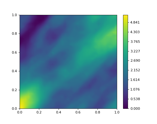
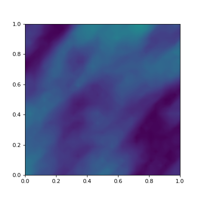
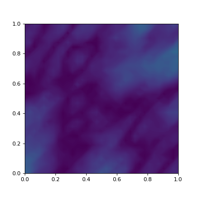
initial guess	ES-model (informed)	VS-model (informed)
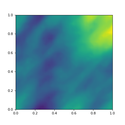
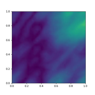
	ES-model (standard)	VS-model (standard)

Figure 3: Pointwise parameter field discrepancy $|m_{\scriptscriptstyle\text{true}}-m_{\mathrm{MAP}}|$ (left and center columns) and $|m_{\scriptscriptstyle\text{true}}-m_{\mathrm{guess}}|$ initial guess (top left) when using the informed (top) and standard (bottom) priors with the energy and variogram scores. The Monte Carlo sample size is 64 in all panels. High discrepancy is indicated by light green, low discrepancy by dark blue.

Table 1 shows the RMSE and SSIM and its 3 components, computed between the parameters $m_{\scriptscriptstyle\text{true}}$ and $m_{\rm MAP}$. As expected, being in the informed prior case leads to smaller RMSE and better SSIM for the inverted parameter, in other words, better overall performance. Additionally, the contrast term, which is related to the variance of each signal, is well captured by the three scores and by both types of priors (standard and informed). In particular, we note that the use of standard priors degrades the capture of the intensity of the parameters given by the luminance term. As expected, the VS-model and HS-model perform better than the ES-model at capturing the covariance between the two parameters $m_{\scriptscriptstyle\text{true}}$ and $m_{\rm MAP}$ (structure term).

	Samples	Luminance	Contrast	Structure	SSIM	RMSE
Model	(a) Informed prior
ES	1	0.847	1	0.698	0.591	1.137
	4	0.801	0.989	0.797	0.631	1.134
	8	0.824	0.995	0.777	0.637	1.108
	32	0.803	0.996	0.765	0.612	1.155
	64	0.793	0.992	0.757	0.596	1.176
	128	0.786	0.995	0.759	0.594	1.187
VS	1	0.825	0.997	0.755	0.621	1.124
	4	0.955	0.976	0.868	0.809	0.696
	8	0.966	0.967	0.859	0.803	0.66
	32	0.98	0.948	0.848	0.788	0.617
	64	0.982	0.939	0.846	0.78	0.612
	128	0.987	0.947	0.855	0.799	0.574
HS	1	0.837	1	0.722	0.605	1.136
	4	0.935	0.981	0.868	0.796	0.765
	8	0.947	0.979	0.853	0.737	0.737
	32	0.958	0.973	0.833	0.776	0.719
	64	0.960	0.966	0.83	0.769	0.716
	128	0.962	0.972	0.836	0.782	0.697
Model	(b) Standard prior
ES	1	-0.729	0.997	0.442	-0.321	2.988
	4	-0.336	1	0.371	-0.125	2.535
	8	-0.29	0.999	0.385	-0.112	2.483
	32	-0.386	0.989	0.469	-0.179	2.538
	64	-0.283	0.985	0.469	-0.131	2.43
	128	-0.371	0.996	0.412	-0.152	2.548
VS	1	-0.828	0.991	0.527	-0.432	3.146
	4	-0.547	0.999	0.447	-0.245	2.737
	8	0.268	0.998	0.363	0.097	2.017
	32	0.412	0.995	0.46	0.189	1.8
	64	0.839	0.995	0.43	0.359	1.3
	128	0.863	0.999	0.402	0.346	1.292
HS	1	-0.85	0.989	0.501	-0.421	3.202
	4	-0.351	0.998	0.42	-0.147	2.527
	8	-0.192	1	0.406	-0.078	2.385
	32	-0.223	0.989	0.485	-0.107	2.37
	64	-0.023	0.992	0.465	-0.011	2.194
	128	-0.074	0.998	0.421	-0.031	2.265

Table 1: Quality of the reconstruction of the parameter field (i.e., the MAP point $m_{\rm MAP}$) measured by different metrics with informed (a) and standard (b) priors. The Samples column lists the number of Monte Carlo samples used to approximate the stochastic right-hand side was. The Luminance column shows the consistency in terms of intensity of the two signals; the Contrast column represents the matching of variance of the two signals; and the Structure column shows the covariance matching between the two signals. The SSIM column—the product of the luminance, contrast, and structure—is a global measure of consistency of the two studied quantities. One expects the SSIM and its factor components to be as close to 1 as possible. The last column, RMSE, shows the root mean squared errors between the two signals, one expects the RMSE to be as small as possible. This table shows that in the proposed setup of informed priors enables better results in terms of SSIM and RMSE and that the VS-model tends to provide a better matching between the true and estimated parameter field. The variance of each signal tends to be well captured by all models.

Comparison between $\mathcal{F}(m)$ and ${\boldsymbol{d}_{\scriptscriptstyle\text{obs}}}$

To assess the quality and statistical properties of the observables generated by the model, in Figure 4 we show the rank histograms reflecting the statistical consistency between the true observables ${\boldsymbol{d}_{\scriptscriptstyle\text{obs}}}$ and the generated ones $\mathcal{F}(m)$. The results show that the standard priors (right row) provide a better calibration between ${\boldsymbol{d}_{\scriptscriptstyle\text{obs}}}$ and $\mathcal{F}(m)$ than do the informed priors (central row). Additionally, the results show that the ES-model (top row) generates calibrated $\mathcal{F}(m)$. This is not unexpected since the energy score is known for discriminating between the intensity of the signals it compares [44]. The VS-model (center row) does not present good calibration results. This result is not unexpected either since the variogram score is known for not capturing the intensity of the signals it compares [49]. We remark that the observables from the VS-model show some overdispersion (bell-shaped histogram). The hybrid score seems to take advantage of the properties of the energy score in terms of calibration and thus appears to be a good compromise between the ES-model and the VS-model. We note that the rank histograms do not assess the correlation structure of the data. In that context we investigate in the following indexes that measure the spatial data structure.

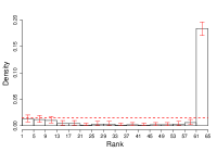
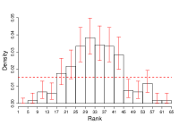
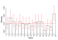
initial guess	ES (informed prior)	ES (standard prior)
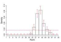
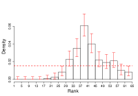
	VS (informed prior)	VS (standard prior)
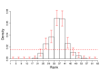
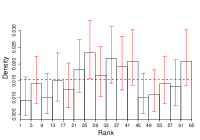
	HS (informed prior)	HS (standard prior)

Figure 4: Rank histogram between ${\boldsymbol{d}_{\scriptscriptstyle\text{obs}}}$ and $\mathcal{F}(m)$. From left to right: guess, $\mathcal{F}(m)$ obtained by using the informed prior, and $\mathcal{F}(m)$ obtained by using the standard prior. From top to bottom: ES-model; VS-model; HS-model. The horizontal line is the perfect uniform histogram that represents a perfect match between ${\boldsymbol{d}_{\scriptscriptstyle\text{obs}}}$ and $\mathcal{F}(m)$. Red whiskers show $\%95$-confidence intervals associated with the estimated count histogram. The closer to the uniform histogram, the better the consistency between ${\boldsymbol{d}_{\scriptscriptstyle\text{obs}}}$ and $\mathcal{F}(m)$. Histograms are obtained for simulations with 64 samples.

In order to investigate the spatial structure of the observables, a metric assessing structural feature, namely, the SSIM, is computed. For each generated sample, in order to assess the overall error between the signals, the SSIM and RMSE are computed between the true and the recovered observable. The values of the metrics are summarized in boxplots in Figure 5. Comparable to Figure 4, Figure 5 shows that the ES-model and HS-model provide better results than does the VS-model in terms of recovering the observables $\mathcal{F}(m)$. The metrics tend to have more variability for the VS-model and HS-model when the number of samples increases. This variability likely comes from the overdispersion of the outputs of the VS-model. We note, however, that the overall range of the bulk of the distribution (box) stays reasonably narrow. The hybrid score thus appears to be a good compromise between the ES-model and VS-model.

RMSE
ES (standard prior)	VS (standard prior)	HS (standard prior)
ES (informed prior)	VS (informed prior)	HS (informed prior)
SSIM
ES (standard prior)	VS (standard prior)	HS (standard prior)
ES (informed prior)	VS (informed prior)	HS (informed prior)

Figure 5: RMSE (two upper rows) and SSIM (two lower rows) between ${\boldsymbol{d}_{\scriptscriptstyle\text{obs}}}$ and each sample of $\mathcal{F}(m)$. Left to right: ES-model; VS-model; HS-model. Models are run with informed and standard priors. The number of samples of the right-hand side varies for each model (N = 4, 8, 32, 64, 128). The RMSE is expected to be as close to 0 as possible, whereas an ideal SSIM would be as close to 1 as possible.

As a conclusion, the overall method shows a wide range of results in this experimental setup. In terms of capturing the parameter field and the intensity and the variability of $m$, the VS- and HS- scores show better agreement with the true one than does the ES-based model. For observables, however, the ES-model shows good results in capturing statistics of the data ${\boldsymbol{d}_{\scriptscriptstyle\text{obs}}}$. As expected, the informed priors help capture the parameter $m$ better, as seen on Table 1 whereas the standard prior case gives a better calibration between ${\boldsymbol{d}_{\scriptscriptstyle\text{obs}}}$ and $\mathcal{F}(m)$ and more accurate intensity and structure of $\mathcal{F}(m)$ (see Figures 4 and 5) arguably by relaxing the parameter constrained through the prior.

5 Model problem 2: Parameter identification in power grid applications governed by DAEs

Next we probe the proposed scores on a power grid inverse model problem governed by an index-1 DAE system. This model incorporates an electromagnetic machine, a slack bus, and a stochastic load as illustrated in Figure 6.

Figure 6: Power grid diagram.

We model the power grid using the generator, current, and network equations [47], namely,

(24a) $$\begin{cases}\dot{x}&=f(x,y;m)\\ 0&=g(x,y;\xi)\end{cases}\Rightarrow F(u,m;\xi)=0~{}\textnormal{a.s.}\,,~{}u=[x,y]^{T}\,.$$

Here $x$ is associated mainly with generators, and $y$ represents current (part of the generator equations) and the network equations (Kirchhoff). The full set of equations is given in Appendix A. The unknown (or inversion) parameter here is $m$ and represents the generator inertia, which is one dimensional in this example. This parameter can be interpreted as how fast the generator reacts to fluctuations in the network. In our case $\xi=[P,Q]^{T}$ represents fluctuations in the load, where $P$ and $Q$ represent the real and imaginary resistive components, respectively.

In recent work we have explored estimating the inertia parameters in a standard 9-bus system given a single known disturbance in the load from synthetic bus voltage observations [40]. In this study we pose the problem as having a small signal disturbance in the load, which is a discrete process in time. This problem now describes a realistic behavior of small-scale consumers drawing power from the grid in an unobserved fashion. What we consider to be known is the distribution of the probabilistic load process. Moreover, we assume that we measure the power flow (or voltage) at one of the buses (see Figure 6).

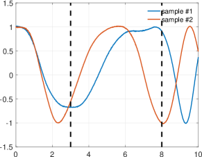
(a) $V_{r}$ simulated

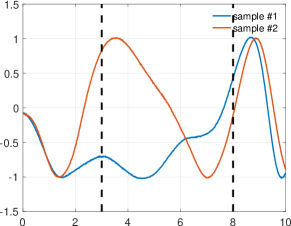
(b) $V_{i}$ simulated

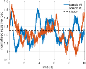
(c) $P$ time series

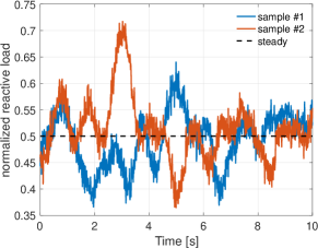
(d) $Q$ time series

Figure 7: Voltage with (a) real and (b) imaginary parts at the measurement location for two samples. Load noise around the stationarity baseline for the (c) resitive and (d) reactive components.

5.1 Computational experiment

We start with the system at dynamic steady state having $\frac{\partial x}{\partial t}=\frac{\partial y}{\partial t}=0$ and $\xi=\left[\overline{P},\overline{Q}\right]^{T}=[1.25,0.5]^{T}$. The system is integrated with backward Euler with stochastic forcing. This discretization is then equivalent to first-order weak convergence in the mean square error sense of the stochastic DAE. Higher-order methods have been used as well, without noticing any qualitative differences for our current setup. The time series generated by the stochastic forcing is given by two independent stationary processes with known distribution $\pi_{\mbox{\tiny$\xi$}}$:

(25) $$\xi=[P,Q]^{T},P(t)\sim{\cal N}\left(\overline{P},0.1^{2}\,\rm{k}(h)\,\right),~{}Q(t)\sim{\cal N}\left(\overline{Q},0.05^{2}\,\rm{k}(h)\,\right),~{}\rm{k}(h)=e^{-\frac{h^{2}}{0.002}}+0.1,$$

where $h=t-t^{\prime}$ and, as before, $\mathrm{Cov}(P(t),P(t^{\prime}))=\rm{k}(h)$. Some realizations of these time series are shown in Figure 7(c)-7(d).

The simulation time is $T=10$ seconds, with a time step of ${\Delta t}=10^{-2}$ (10 ms). From the 10-second window we extract 5 seconds (seconds 3 to 8) to avoid initialization or mixture issues. We consider an ensemble of 1,000 samples integrated with this time step, with ${N_{s}}=800$ being considered as numerical simulations and $n=1,2,\dots,200$ set aside for observations. In this experiment we do not consider observational noise ($\varepsilon_{\rm obs}\equiv 0$) and do not need to use any regularization; this is equivalent to an uninformative or flat prior. The optimization problem becomes a univariate unconstrained program, and therefore we approximate the gradient with finite differences. Nevertheless, one can compute the gradients via adjoints as has been done for model problem 1 in Section 4 as well.

5.2 Analysis of the results

The time-dependent setting allows us to analyze different aspects of the inverse problem solution. For instance, in the steady-state case such as the first model problem, the spatial domain is fixed, and in general so is the number of observations. In the unsteady example, one typically has control over the observation window. To this end, we begin by exploring the effect of adding observations to the inference process and thus using the mean score (10). Specifically, we compute the score values at integer values of the parameter, from 1 to 35, and use 1 to 200 batches of observations or validation samples. In other words we explore the mean score values $S_{n}$ with $n=1,\dots,200$; i.e., ${\boldsymbol{d}_{\scriptscriptstyle\text{obs}}}^{(1,\dots,n)}=[{\boldsymbol{d}_{\scriptscriptstyle\text{obs}}}^{(1)},{\boldsymbol{d}_{\scriptscriptstyle\text{obs}}}^{(2)},\dots\boldsymbol{d}_{\scriptscriptstyle\text{obs}}^{(n)}]^{\top}\in\mathbb{R}^{n\times M}$. One batch is the time series obtained under a stochastic forcing realization. Each batch is the result of a 5-second simulation, and this assumes that the distribution is stationary for the entire inference window; i.e., the distributions do not change over time. The observations of the voltage $x_{11}$ and $x_{14}$ corresponding to the middle bus are taken at every time step.

We illustrate the results in Figure 8 for the ES-model and VS-model computed with respect to two exact values of the parameter, 10 and 20, respectively. We observe that both the energy and variogram scores converge to the exact value, with the variogram score converging much faster than the energy score especially when the exact value of the parameter is 10. We also remark that convergence guarantees are not easy to ascertain a priori; as reflected in the figure, a different number of observations are necessary in order to reach an accurate conclusion. One possible strategy to mitigate this issue is to use two different scores and observe the system until they are in agreement and do not change with additional observations.

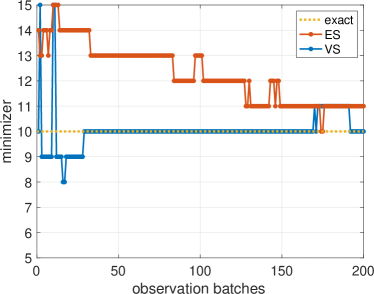
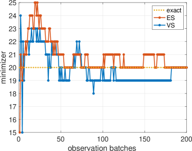
Figure 8: Grid search of the minimizer as a function of observation batches. The exact parameter value is 10 for the left panel and 20 for right one. As the number of observations increases, the minimizer converges to the true value.

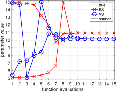
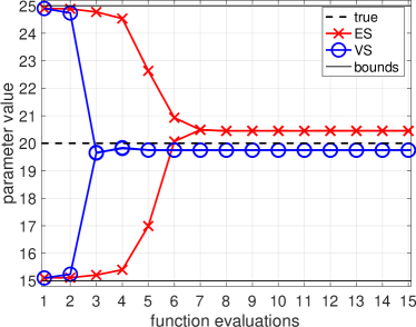
Figure 9: Reconstructed parameter for $m_{\scriptscriptstyle\text{true}}=10$ (left) and $m_{\scriptscriptstyle\text{true}}=20$ (right). The results obtained with the energy score are shown in red (cross) and for the variogram score in blue (circles). The bounds $m_{\scriptscriptstyle\text{true}}\,\pm\,5$ used in the optimization solver are shown with a black solid line. Two experiments are carried out for each score with the initial guess being the high and low bound values.

The numerical results are carried out in Matlab using the default optimization solver. In Figure 9 we show the reconstructed parameter values as a function of function evaluations for the exact parameter values (black dashed line) 10 (left) and 20 (right). The results for the energy score are shown in red (cross) and for the variogram score in blue (circles). The bounds set to truth$\,\pm\,5$ used in the optimization solver are shown with a black solid line. This figure shows that with both scores the optimization solver converges to a relatively good estimate of the exact parameter value in a relatively small number of function evaluations.

6 Conclusions

We have presented a statistical treatment of inverse problems governed by physics-based models with stochastic inputs. The goal of this study is to quantify the quality of the inverted parameter field, measured by a comparison with the “truth,” and the quality of the recovered observable: for example, given the inverted parameter field, quantify how well we fit the distribution of the observable. The end goal of our study is to introduce an inverse problem formulation that facilitates the integration of data with physics-based models in order to quantify the uncertainties in model predictions. To this end, inspired from statistics, we propose to replace the traditional least-squares minimization problem—which minimizes the norm of the misfit between data and observables—with a set of loss functions that describes quantitatively the distance between the distributions of model generated data and the distribution of observational data. We refer to these metrics as scores, as known in the statistics community.

To compute the maximum utility or a posteriori point for the proposed inverse problem, we solve an optimization problem constrained by the physics-based models under stochastic inputs with a quasi-Newton limited-memory algorithm. For efficient calculation of the gradient of the objective with respect to the inversion parameters, we derive adjoint-based expressions. Several challenges are associated with solving such optimization problems. First, these inverse problems are large scale, stemming from discretization of the parameter field in the case of PDE-based models or the size of the power grid network. Second, although we employ an efficient method to calculate derivatives, the number of adjoint solves increases with the number of samples and are coupled. As we indicated above, however, the communication during the adjoint calculations follows a fixed pattern and can be optimized for, arguably resulting in overall scalable strategies. Third, structured error in measurements (data) requires special attention, and convergence guarantees are not easy to ascertain a priori. Nevertheless, as we illustrate in the second model (see Fig. 8), one can use multiple sets of data to ascertain and mitigate potential convergence issues.

We have studied the performance of the proposed formulation in the context of two applications: a coefficient field inversion for subsurface flow governed by an elliptic PDE with a stochastic source and a parameter inversion for power grid governed by DAEs. In both cases the goal was to obtain predictive probabilistic models that explain the data.

The submitted manuscript has been created by UChicago Argonne, LLC, Operator of Argonne National Laboratory (“Argonne”). Argonne, a U.S. Department of Energy Office of Science laboratory, is operated under Contract No. DE-AC02-06CH11357. The U.S. Government retains for itself, and others acting on its behalf, a paid-up nonexclusive, irrevocable worldwide license in said article to reproduce, prepare derivative works, distribute copies to the public, and perform publicly and display publicly, by or on behalf of the Government. The Department of Energy will provide public access to these results of federally sponsored research in accordance with the DOE Public Access Plan. http://energy.gov/downloads/doe-public-access-plan.

Appendix A Power grid equations

Below we present the equations extracted from [47] for the power grid example discussed in Sec. 5. The one generator 3-bus system is described by index-1 DAEs. Here we have 7 differential equations and 8 algebraic equations. The differential variables are the first seven variables, with the rest being algebraic.

$$\dot{x}_{1}= -376.99111843077515+x_{2}$$

$$\frac{m}{23.64}\dot{x}_{2}= 47.70113037725341-0.09968102073365231x_{2}-7.974481658692184(x_{4}x_{8}+x_{3}x_{9}+0.0361x_{8}x_{9})$$

$$\dot{x}_{3}= 0.11160714285714285(x_{5}-x_{3})-0.009508928571428571x_{8}$$

$$\dot{x}_{4}= -3.2258064516129035x_{4}+1.0938709677419356x_{9}$$

$$\dot{x}_{5}= -0.012420382165605096\exp(1.555x_{5})+3.1847133757961785(x_{7}-x_{5})$$

$$\dot{x}_{6}= 0.5142857142857145x_{5}-2.857142857142857x_{6}$$

$$\dot{x}_{7}= 109.644151839917-18x_{5}+100x_{6}-5x_{7}-100\sqrt{x_{10}^{2}+x_{13}^{2}}$$

$$0= x_{8}+16.44736842105263(\cos(x_{1})x_{10}+\sin(x_{1})x_{13}-x_{3})$$

$$0= x_{9}+10.319917440660475(x_{4}-\sin(x_{1})x_{10}+\cos(x_{1})x_{13})$$

$$0= \sin(x_{1})x_{8}+\cos(x_{1})x_{9}-0.030140727054618(x_{10}-x_{11})-17.361008783459972(x_{13}-x_{14})$$

$$0= 0.030140727054618x_{10}-1.395328440365198x_{11}+1.36518771331058x_{12}+17.361058783459974x_{13}-$$

$$\quad 28.877104346599904x_{14}+11.60409556313993x_{15}$$

$$0= 1.36518771331058(x_{11}-x_{12})+11.60409556313993x_{14}-11.516095563139931x_{15}-\frac{Px_{12}}{x_{12}^{2}+x_{15}^{2}}-\frac{Qx_{15}}{x_{12}^{2}+x_{15}^{2}}$$

$$0= -(\cos(x_{1})x_{8})+\sin(x_{1})x_{9}+17.361008783459972(x_{10}-x_{11})-0.030140727054618(x_{13}-x_{14})$$

$$0= -17.361058783459974x_{10}+28.877104346599904x_{11}-11.60409556313993x_{12}+0.030140727054618x_{13}$$

$$\quad-1.395328440365198x_{14}+1.36518771331058x_{15}$$

$$0= -11.60409556313993x_{11}+11.516095563139931x_{12}+1.36518771331058(x_{14}-x_{15})+\frac{Qx_{12}}{x_{12}^{2}+x_{15}^{2}}-\frac{Px_{15}}{x_{12}^{2}+x_{15}^{2}}$$

The initial condition that gives a steady state is given by $x(t_{0})=[0.391057483977274,376.9911184307751,\\ 1.022092319747551,0.308311065534821,1.107019848098437,0.199263572657719,1.12883036798339,0.996801975949364,\\ 0.909203967958775,1.04,1.006755413658047,0.938198590465838,0,-0.070244002800643,-0.166824934470857]^{T}$, here $P=1.25$ and $Q=0.5$.

The stochastic noise is characterized by $\xi=[P,Q]^{T}$ and the parameter sought is $m$, while observing the voltage at the slack bus, $x_{11}$ and $x_{14}$.

References

- [1] A. Alexanderian, N. Petra, G. Stadler, and O. Ghattas, A fast and scalable method for A-optimal design of experiments for infinite-dimensional Bayesian nonlinear inverse problems, SIAM Journal on Scientific Computing, 38 (2016), pp. A243–A272, https://doi.org/10.1137/140992564, http://dx.doi.org/10.1137/140992564.
- [2] J. L. Anderson, A method for producing and evaluating probabilistic forecasts from ensemble model integrations, Journal of Climate, 9 (1996), pp. 1518–1530.
- [3] G. Bal, I. Langmore, and Y. Marzouk, Bayesian inverse problems with Monte Carlo forward models, Inverse Problems & Imaging, 7 (2013), p. 81, https://doi.org/10.3934/ipi.2013.7.81, http://aimsciences.org//article/id/d904b995-d45b-482c-b697-3347afcb9c98.
- [4] S. Balay, K. Buschelman, W. D. Gropp, D. Kaushik, M. Knepley, L. C. McInnes, B. F. Smith, and H. Zhang, PETSc home page, 2001. http://www.mcs.anl.gov/petsc.
- [5] S. Balay, K. Buschelman, W. D. Gropp, D. Kaushik, M. G. Knepley, L. C. McInnes, B. F. Smith, and H. Zhang, PETSc Web page, 2009. http://www.mcs.anl.gov/petsc.
- [6] S. Baran, Probabilistic wind speed forecasting using bayesian model averaging with truncated normal components, Computational Statistics & Data Analysis, 75 (2014), pp. 227–238.
- [7] S. Baran and S. Lerch, Log-normal distribution based ensemble model output statistics models for probabilistic wind-speed forecasting, Quarterly Journal of the Royal Meteorological Society, 141 (2015), pp. 2289–2299.
- [8] E. Bernton, P. E. Jacob, M. Gerber, and C. P. Robert, Inference in generative models using the wasserstein distance, arXiv preprint arXiv:1701.05146, (2017).
- [9] A. Borzì and V. Schulz, Computational Optimization of Systems Governed by Partial Differential Equations, SIAM, 2012.
- [10] A. Borzì and G. Von Winckel, Multigrid methods and sparse-grid collocation techniques for parabolic optimal control problems with random coefficients, SIAM Journal on Scientific Computing, 31 (2009), pp. 2172–2192.
- [11] T. Bui-Thanh, O. Ghattas, J. Martin, and G. Stadler, A computational framework for infinite-dimensional Bayesian inverse problems Part I: The linearized case, with application to global seismic inversion, SIAM Journal on Scientific Computing, 35 (2013), pp. A2494–A2523, https://doi.org/10.1137/12089586X.
- [12] R. H. Byrd, J. Nocedal, and R. B. Schnabel, Representations of quasi-newton matrices and their use in limited memory methods, Mathematical Programming, 63 (1994), pp. 129–156, https://doi.org/10.1007/BF01582063, http://dx.doi.org/10.1007/BF01582063.
- [13] T. Dupont, J. Hoffman, C. Johnson, R. Kirby, M. Larson, A. Logg, and R. Scott, The FEniCS project, tech. report, 2003.
- [14] C. A. T. Ferro, Measuring forecast performance in the presence of observation error, Quarterly Journal of the Royal Meteorological Society, 143 (2017), pp. 2665–2676, https://doi.org/10.1002/qj.3115, http://dx.doi.org/10.1002/qj.3115.
- [15] Y. Gel, A. E. Raftery, and T. Gneiting, Calibrated probabilistic mesoscale weather field forecasting: The geostatistical output perturbation method, Journal of the American Statistical Association, 99 (2004), pp. 575–583.
- [16] M. Giles, Multilevel Monte Carlo methods, Acta Numerica, 24 (2015), pp. 259–328.
- [17] T. Gneiting and M. Katzfuss, Probabilistic forecasting, Annual Review of Statistics and Its Application, 1 (2014), pp. 125–151.
- [18] T. Gneiting and A. E. Raftery, Strictly proper scoring rules, prediction, and estimation, Journal of the American Statistical Association, 102 (2007), pp. 359–378.
- [19] T. Gneiting, A. E. Raftery, A. H. Westveld III, and T. Goldman, Calibrated probabilistic forecasting using ensemble model output statistics and minimum CRPS estimation, Monthly Weather Review, 133 (2005), pp. 1098–1118.
- [20] T. Gneiting, L. I. Stanberry, E. P. Grimit, L. Held, and N. A. Johnson, Assessing probabilistic forecasts of multivariate quantities, with an application to ensemble predictions of surface winds, Test, 17 (2008), pp. 211–235.
- [21] M. Gunzburger, N. Jiang, and Z. Wang, A second-order time-stepping scheme for simulating ensembles of parameterized flow problems, Computational Methods in Applied Mathematics, (2017).
- [22] M. Gunzburger, C. Webster, and G. Zhang, Stochastic finite element methods for partial differential equations with random input data, Acta Numerica, 23 (2014), p. 521–650, https://doi.org/10.1017/S0962492914000075.
- [23] M. Hairer, Introduction to Stochastic PDEs. Lecture Notes, 2009.
- [24] T. M. Hamill, Interpretation of rank histograms for verifying ensemble forecasts, Monthly Weather Review, 129 (2001), pp. 550–560.
- [25] J. Kaipio and V. Kolehmainen, Bayesian Theory and Applications, Oxford University Press, 2013, ch. Approximate Marginalization Over Modeling Errors and Uncertainties in Inverse Problems, pp. 644–672.
- [26] J. Kaipio and E. Somersalo, Statistical and Computational Inverse Problems, vol. 160 of Applied Mathematical Sciences, Springer-Verlag, New York, 2005.
- [27] E. Kalnay, Atmospheric Modeling, Data Assimilation and Predictability, Cambridge University Press, 2003.
- [28] R. Kass and A. Raftery, Bayes factors, Journal of the American Statistical Association, 90 (1995), pp. 773–795, https://doi.org/10.1080/01621459.1995.10476572.
- [29] S. Lerch and T. L. Thorarinsdottir, Comparison of non-homogeneous regression models for probabilistic wind speed forecasting, Tellus A: Dynamic Meteorology and Oceanography, 65 (2013), p. 21206.
- [30] H. Lie, T. Sullivan, and A. Teckentrup, Random forward models and log-likelihoods in Bayesian inverse problems, ArXiv e-prints, (2017), https://arxiv.org/abs/1712.05717.
- [31] A. Logg, K.-A. Mardal, and G. N. Wells, eds., Automated Solution of Differential Equations by the Finite Element Method, vol. 84 of Lecture Notes in Computational Science and Engineering, Springer, 2012.
- [32] D. Maraun, F. Wetterhall, A. Ireson, R. Chandler, E. Kendon, M. Widmann, S. Brienen, H. Rust, T. Sauter, M. Themeßl, et al., Precipitation downscaling under climate change: Recent developments to bridge the gap between dynamical models and the end user, Reviews of Geophysics, 48 (2010).
- [33] J.-M. Marin, P. Pudlo, C. P. Robert, and R. J. Ryder, Approximate bayesian computational methods, Statistics and Computing, 22 (2012), pp. 1167–1180.
- [34] S. Mattis, T. Butler, C. Dawson, D. Estep, and V. Vesselinov, Parameter estimation and prediction for groundwater contamination based on measure theory, Water Resources Research, 51 (2015), pp. 7608–7629.
- [35] P. Naveau and J. Bessac, Forecast evaluation with imperfect observations and imperfect models. 2018.
- [36] R. Nicholson, N. Petra, and P. J. Kaipio, Estimation of the Robin coefficient field in a Poisson problem with uncertain conductivity field, Inverse Problems, 34 (2018), p. 115005.
- [37] J. Nocedal and S. J. Wright, Numerical Optimization, Springer, New York, 2nd ed., 2006.
- [38] C. G. Petra, A memory-distributed quasi-Newton solver for nonlinear programming problems with a small number of general constraints, in review to the Journal of Parallel and Distributed Computed, (2017).
- [39] N. Petra, J. Martin, G. Stadler, and O. Ghattas, A computational framework for infinite-dimensional Bayesian inverse problems: Part II. Stochastic Newton MCMC with application to ice sheet inverse problems, SIAM Journal on Scientific Computing, 36 (2014), pp. A1525–A1555.
- [40] N. Petra, C. Petra, Z. Zhang, E. Constantinescu, and M. Anitescu, A Bayesian approach for parameter estimation with uncertainty for dynamic power systems, IEEE Transactions on Power Systems, 32 (2017), pp. 2735–2743, https://doi.org/10.1109/TPWRS.2016.2625277.
- [41] N. Petra and G. Stadler, Model variational inverse problems governed by partial differential equations, Tech. Report 11-05, The Institute for Computational Engineering and Sciences, The University of Texas at Austin, 2011.
- [42] J. Pfanzagl, On the measurability and consistency of minimum contrast estimates, Metrika, 14 (1969), pp. 249–272.
- [43] P. Pinson and R. Girard, Evaluating the quality of scenarios of short-term wind power generation, Applied Energy, 96 (2012), pp. 12–20.
- [44] P. Pinson and J. Tastu, Discrimination ability of the energy score, tech. report, Technical University of Denmark, 2013.
- [45] A. E. Raftery, T. Gneiting, F. Balabdaoui, and M. Polakowski, Using Bayesian model averaging to calibrate forecast ensembles, Monthly Weather Review, 133 (2005), pp. 1155–1174.
- [46] E. Rosseel and G. Wells, Optimal control with stochastic PDE constraints and uncertain controls, Computer Methods in Applied Mechanics and Engineering, 213 (2012), pp. 152–167.
- [47] P. W. Sauer and M. Pai, Power system dynamics and stability, Prentice Hall Upper Saddle River, NJ, 1998.
- [48] M. Scheuerer, Probabilistic quantitative precipitation forecasting using ensemble model output statistics, Quarterly Journal of the Royal Meteorological Society, 140 (2014), pp. 1086–1096.
- [49] M. Scheuerer and T. M. Hamill, Variogram-based proper scoring rules for probabilistic forecasts of multivariate quantities, Monthly Weather Review, 143 (2015), pp. 1321–1334.
- [50] M. Scheuerer and D. Möller, Probabilistic wind speed forecasting on a grid based on ensemble model output statistics, The Annals of Applied Statistics, 9 (2015), pp. 1328–1349.
- [51] M. A. Semenov and E. M. Barrow, Use of a stochastic weather generator in the development of climate change scenarios, Climatic change, 35 (1997), pp. 397–414.
- [52] J. M. L. Sloughter, T. Gneiting, and A. E. Raftery, Probabilistic wind speed forecasting using ensembles and Bayesian model averaging, Journal of the American Statistical Association, 105 (2010), pp. 25–35.
- [53] A. M. Stuart, Inverse problems: A Bayesian perspective, Acta Numerica, 19 (2010), pp. 451–559.
- [54] T. Thorarinsdottir, T. Gneiting, and N. Gissibl, Using proper divergence functions to evaluate climate models, SIAM/ASA Journal on Uncertainty Quantification, 1 (2013), pp. 522–534.
- [55] T. L. Thorarinsdottir and T. Gneiting, Probabilistic forecasts of wind speed: ensemble model output statistics by using heteroscedastic censored regression, Journal of the Royal Statistical Society: Series A (Statistics in Society), 173 (2010), pp. 371–388.
- [56] F. Tröltzsch, Optimal Control of Partial Differential Equations: Theory, Methods and Applications, vol. 112 of Graduate Studies in Mathematics, American Mathematical Society, 2010.
- [57] U. Villa, N. Petra, and O. Ghattas, hIPPYlib: an Extensible Software Framework for Large-scale Deterministic and Bayesian Inversion, (2016), https://doi.org/10.5281/zenodo.596931, http://hippylib.github.io.
- [58] U. Villa, N. Petra, and O. Ghattas, hIPPYlib: An extensible software framework for large-scale inverse problems, Journal of Open Source Software, 3 (2018), p. 115005, https://doi.org/10.21105/joss.00940.
- [59] C. R. Vogel, Computational Methods for Inverse Problems, Frontiers in Applied Mathematics, Society for Industrial and Applied Mathematics (SIAM), Philadelphia, PA, 2002.
- [60] C. R. Vogel, Computational methods for inverse problems, vol. 23, Siam, 2002.
- [61] Z. Wang, A. C. Bovik, H. R. Sheikh, and E. P. Simoncelli, Image quality assessment: from error visibility to structural similarity, IEEE transactions on image processing, 13 (2004), pp. 600–612.
- [62] N. Zabaras and B. Ganapathysubramanian, A scalable framework for the solution of stochastic inverse problems using a sparse grid collocation approach, Journal of Computational Physics, 227 (2008), pp. 4697–4735.
- [63] C. Zhang, J. Butepage, H. Kjellstrom, and S. Mandt, Advances in variational inference, IEEE transactions on pattern analysis and machine intelligence, (2018).