Global minima for optimal control of the obstacle problem

Abstract

An optimal control problem subject to an elliptic obstacle problem is studied. We obtain a numerical approximation of this problem by discretising the PDE obtained via a Moreau–Yosida type penalisation. For the resulting discrete control problem we provide a condition that allows to decide whether a solution of the necessary first order conditions is a global minimum. In addition we show that the corresponding result can be transferred to the limit problem provided that the above condition holds uniformly in the penalisation and discretisation parameters. Numerical examples with unique global solutions are presented.

Key words. Optimal control, obstacle problem, Moreau–Yosida penalisation, finite elements, global solution.
Mathematics Subject Classification. 49J20, 49M05, 49M20, 65M15, 65M60.

1 Introduction

In this paper we are concerned with the following distributed optimal control problem for the elliptic obstacle problem

$$(\mathbb{P})\quad\min_{u\in L^{2}(\Omega)}J(u)=\frac{1}{2}\|y-y_{0}\|_{L^{2}(\Omega)}^{2}+\dfrac{\alpha}{2}\|u\|_{L^{2}(\Omega)}^{2}$$

subject to

$$y\in K,\quad\int_{\Omega}\nabla y\cdot\nabla(\phi-y)dx\geq\int_{\Omega}(f+u)(\phi-y)dx\qquad\forall\phi\in K,$$ (1.1)

where

$$K=\{\phi\in H^{1}_{0}(\Omega)\,|\,\phi(x)\geq\psi(x)\mbox{ a.e. in }\Omega\}.$$

Furthermore, $\displaystyle\Omega\subset\mathbb{R}^{d}\,(d=2,3)$ is a bounded polyhedral domain, $\displaystyle\psi\in H^{1}_{0}(\Omega)\cap H^{2}(\Omega)$ is the given obstacle, $\displaystyle y_{0},f\in L^{2}(\Omega)$ and $\displaystyle\alpha>0$.
It is well–known that for a given function $\displaystyle u\in L^{2}(\Omega)$ the variational inequality (1.1) has a unique solution $\displaystyle y\in K$ and using standard arguments (cf. [14, Theorem 2.1]) one obtains the existence of a solution of $\displaystyle(\mathbb{P})$. However, a major issue in the analysis and numerical approximation of $\displaystyle(\mathbb{P})$ is the fact that the mapping $\displaystyle u\mapsto y$ is in general not Gâteaux differentiable, so that the derivation of necessary first order optimality conditions becomes a difficult task. A common approach in order to handle this difficulty consists in approximating (1.1) by a sequence of penalised or regularised problems and then to pass to the limit, see e.g. [3], [14], [8], [6], [7], [9], [15] and [12]. In our work we employ a Moreau–Yosida type penalisation of the obstacle problem resulting in the following optimal control problem depending on the parameter $\displaystyle\gamma\gg 1$:

$$(\mathbb{P}^{\gamma})\quad\min_{u\in L^{2}(\Omega)}J^{\gamma}(u)=\frac{1}{2}\|y-y_{0}\|_{L^{2}(\Omega)}^{2}+\dfrac{\alpha}{2}\|u\|_{L^{2}(\Omega)}^{2}$$

subject to

$$\int_{\Omega}\nabla y\cdot\nabla\phi\,dx+\gamma^{3}\int_{\Omega}[(y-\psi)^{-}]^{3}\,\phi\,dx=\int_{\Omega}(f+u)\phi\,dx\qquad\forall\phi\in H^{1}_{0}(\Omega).$$ (1.2)

Here, $\displaystyle a^{-}=\min(a,0)$. Existence of a solution of $\displaystyle(\mathbb{P}^{\gamma})$ and a detailed convergence analysis as $\displaystyle\gamma\rightarrow\infty$ can be found in [12, Section 3]. For numerical purposes we shall discretise the PDE (1.2) with the help of continuous, piecewise linear finite elements giving rise to a discrete optimisation problem, whose solutions satisfy standard first order optimality conditions. Due to the lack of convexity of the underlying problem it is however not clear whether a computed discrete stationary point is actually a global minimum. Our first main result of this paper establishes for a fixed penalisation parameter and a discrete stationary solution a condition that ensures global optimality, see Theorem 2.2. This condition has the form of an inequality involving the state and the adjoint variable as well as the obstacle. Furthermore, the minimum is unique in case that the inequality is strict. A similar kind of result for control problems subject to a class of semilinear elliptic PDEs has been obtained in [1, 2], but the form of the condition presented here is adapted to the obstacle problem and entirely different from the one proposed in [1, 2]. In Section 3 we consider a sequence of approximate control problems $\displaystyle(\mathbb{P}^{\gamma_{h}}_{h})$ with $\displaystyle h\rightarrow 0$ and $\displaystyle\gamma_{h}\rightarrow\infty$ as $\displaystyle h\rightarrow 0$, where $\displaystyle h$ denotes the grid size. As our second main result we shall prove that a corresponding sequence of discrete stationary points which are uniformly bounded in a suitable sense has a subsequence that converges to a limit satisfying a system of first order optimality conditions, see Theorem 3.1. It turns out that a solution of this system is strongly stationary in the sense of [14] and that we obtain a continuous analogue of the condition mentioned above guaranteeing global optimality of a stationary point, see Theorem 3.2. The only other sufficient condition for optimality which we are aware of can be found in [13, Theorem 5.4], where global optimality is derived from the condition that $\displaystyle y_{0}\leq\psi$, see also [8, Section 5.2]. A sufficient second order optimality condition giving local optimality is derived in [10]. In Section 4 we briefly outline how to apply our theory to a direct discretisation of (1.1). Finally, several numerical examples with unique global solutions are presented in Section 5.

2 Discretisation of $\displaystyle(\mathbb{P})$

Let $\displaystyle\mathcal{T}_{h}$ be an admissible triangulation of $\displaystyle\Omega$ so that

$$\bar{\Omega}=\bigcup_{T\in\mathcal{T}_{h}}\bar{T}.$$

We denote by $\displaystyle x_{1},\ldots,x_{n}$ the interior and by $\displaystyle x_{n+1},\ldots,x_{n+m}$ the boundary vertices of $\displaystyle\mathcal{T}_{h}$. Next, let

$$X_{h}:=\{v_{h}\in C^{0}(\bar{\Omega}):v_{h}\mbox{ is a linear polynomial on each }T\in\mathcal{T}_{h}\}$$

be the space of linear finite elements as well as $\displaystyle X_{h0}:=X_{h}\cap H^{1}_{0}(\Omega)$. The standard nodal basis functions are defined by $\displaystyle\phi_{i}\in X_{h}$ with $\displaystyle\phi_{i}(x_{j})=\delta_{ij},i,j=1,\ldots,n+m$. In particular, $\displaystyle\{\phi_{1},\ldots,\phi_{n}\}$ is a basis of $\displaystyle X_{h0}$. We shall make use of the Lagrange interpolation operator

$$I_{h}:C^{0}(\bar{\Omega})\rightarrow X_{h}\quad I_{h}y:=\sum_{j=1}^{n+m}y(x_{j})\phi_{i}.$$

Let us approximate (1.2) as follows: for a given $\displaystyle u\in L^{2}(\Omega)$, find $\displaystyle y_{h}\in X_{h0}$ such that

$$\int_{\Omega}\nabla y_{h}\cdot\nabla\phi_{h}\,dx+\gamma^{3}\int_{\Omega}I_{h}\{[(y_{h}-\psi)^{-}]^{3}\,\phi_{h}\}\,dx=\int_{\Omega}(f+u)\phi_{h}\,dx\quad\forall\,\phi_{h}\in X_{h0}.$$ (2.1)

It is not difficult to show that (2.1) has a unique solution $\displaystyle y_{h}\in X_{h0}$. The variational discretization of Problem $\displaystyle(\mathbb{P}^{\gamma})$ now reads:

$$(\mathbb{P}^{\gamma}_{h})\quad\begin{array}[]{l}\min_{u\in L^{2}(\Omega)}J^{\gamma}_{h}(u):=\frac{1}{2}\|y_{h}-y_{0}\|_{L^{2}(\Omega)}^{2}+\dfrac{\alpha}{2}\|u\|_{L^{2}(\Omega)}^{2}\\ \mbox{ subject to }y_{h}\mbox{ solves (\ref{equation: 3}) }.\end{array}$$

Using standard arguments one obtains:

Lemma 2.1

Suppose that $\displaystyle u_{h}\in L^{2}(\Omega)$ is a local solution of $\displaystyle(\mathbb{P}^{\gamma}_{h})$ with corresponding state $\displaystyle y_{h}\in X_{h0}$. Then there exists an adjoint state $\displaystyle p_{h}\in X_{h0}$ such that

$$\displaystyle\int_{\Omega}\nabla y_{h}\cdot\nabla\phi_{h}dx+\gamma^{3}\int_{\Omega}I_{h}\{[(y_{h}-\psi)^{-}]^{3}\,\phi_{h}\}dx \displaystyle= \displaystyle\int_{\Omega}(f+u_{h})\phi_{h}\,dx\quad\forall\,\phi_{h}\in X_{h0}$$ (2.2)

$$\displaystyle\int_{\Omega}\nabla p_{h}\cdot\nabla\phi_{h}dx+3\gamma^{3}\int_{\Omega}I_{h}\{[(y_{h}-\psi)^{-}]^{2}p_{h}\phi_{h}\}dx \displaystyle= \displaystyle\int_{\Omega}(y_{h}-y_{0})\phi_{h}\,dx\quad\forall\,\phi_{h}\in X_{h0}$$ (2.3)

$$\displaystyle\alpha u_{h}+p_{h} \displaystyle= \displaystyle 0\quad\mbox{ in }\Omega.$$ (2.4)

Note that (2.4) implicitly yields a discretisation of the control variable so that (2.2)–(2.4) is a finite–dimensional system that can be solved using classical nonlinear programming algorithms. However, due to the non-convexity of the problem, it is not clear whether a solution of (2.2)–(2.4) is actually a global minimum of $\displaystyle(\mathbb{P}^{\gamma}_{h})$. Our first main result provides a sufficient condition for a discrete stationary point that guarantees that this is the case. In order to formulate the corresponding condition we introduce $\displaystyle\lambda_{1}$ as the smallest eigenvalue of $\displaystyle-\Delta$ in $\displaystyle\Omega$ subject to homogeneous Dirichlet boundary conditions, i.e.

$$\lambda_{1}=\inf_{\phi\in H^{1}_{0}(\Omega)\setminus\{0\}}\frac{\int_{\Omega}|\nabla\phi|^{2}\,dx}{\int_{\Omega}\phi^{2}\,dx}.$$ (2.5)

In what follows we shall abbreviate $\displaystyle y_{j}=y_{h}(x_{j}),p_{j}=p_{h}(x_{j})$ and $\displaystyle\psi_{j}=\psi(x_{j}),\,j=1,\ldots,n$.

Theorem 2.2

Suppose that $\displaystyle(u_{h},y_{h},p_{h})$ is a solution of (2.2)–(2.4), which satisfies

$$p_{k}\geq 0\quad\forall k\in\{1,\ldots,n\}\mbox{ with }y_{k}-\psi_{k}=0$$ (2.6)

and define

$$\eta:=\min\bigl{(}\min_{y_{j}>\psi_{j}}\frac{p_{j}}{y_{j}-\psi_{j}},\min_{y_{j}<\psi_{j}}\frac{3p_{j}}{\psi_{j}-y_{j}},0\bigr{)}.$$ (2.7)

If

$$|\eta|\leq\alpha\lambda_{1}+\sqrt{\alpha^{2}\lambda_{1}^{2}+\alpha},$$ (2.8)

then $\displaystyle u_{h}$ is a global minimum for Problem $\displaystyle(\mathbb{P}^{\gamma}_{h})$. If the inequality (2.8) is strict, then $\displaystyle u_{h}$ is the unique global minimum.

Proof:.

Let $\displaystyle v\in L^{2}(\Omega)$ be arbitrary and denote by $\displaystyle\tilde{y}_{h}\in X_{h0}$ the solution of

$$\int_{\Omega}\nabla\tilde{y}_{h}\cdot\nabla\phi_{h}dx+\gamma^{3}\int_{\Omega}I_{h}\{[(\tilde{y}_{h}-\psi)^{-}]^{3}\,\phi_{h}\}dx=\int_{\Omega}(f+v)\phi_{h}\,dx\quad\forall\,\phi_{h}\in X_{h0}.$$ (2.9)

A straightforward calculation shows that

$$\displaystyle J^{\gamma}_{h}(v)-J^{\gamma}_{h}(u_{h}) \displaystyle= \displaystyle\frac{1}{2}\|\tilde{y}_{h}-y_{h}\|_{L^{2}(\Omega)}^{2}+\frac{\alpha}{2}\|v-u_{h}\|_{L^{2}(\Omega)}^{2}$$ (2.10)

$$\displaystyle+\int_{\Omega}(y_{h}-y_{0})(\tilde{y}_{h}-y_{h})\,dx+\alpha\int_{\Omega}u_{h}(v-u_{h})\,dx.$$

We deduce from (2.3), (2.2) and (2.9) that

$$\displaystyle\int_{\Omega}(y_{h}-y_{0})(\tilde{y}_{h}-y_{h})\,dx=\int_{\Omega}\nabla p_{h}\cdot\nabla(\tilde{y}_{h}-y_{h})\,dx+3\gamma^{3}\int_{\Omega}I_{h}\{[(y_{h}-\psi)^{-}]^{2}p_{h}(\tilde{y}_{h}-y_{h})\}dx$$ (2.11)

$$\displaystyle= \displaystyle-\gamma^{3}\int_{\Omega}I_{h}\{[(\tilde{y}_{h}-\psi)^{-}]^{3}p_{h}\}dx+\gamma^{3}\int_{\Omega}I_{h}\{[(y_{h}-\psi)^{-}]^{3}p_{h}\}dx+\int_{\Omega}p_{h}(v-u_{h})\,dx$$

$$\displaystyle+3\gamma^{3}\int_{\Omega}I_{h}\{[(y_{h}-\psi)^{-}]^{2}p_{h}(\tilde{y}_{h}-y_{h})\}dx$$

$$\displaystyle= \displaystyle\gamma^{3}\int_{\Omega}I_{h}\{p_{h}r_{h}\}\,dx+\int_{\Omega}p_{h}(v-u_{h})\,dx,$$

where

$$\displaystyle r_{h} \displaystyle= \displaystyle-[(\tilde{y}_{h}-\psi)^{-}]^{3}+[(y_{h}-\psi)^{-}]^{3}+3[(y_{h}-\psi)^{-}]^{2}(\tilde{y}_{h}-y_{h})$$

$$\displaystyle= \displaystyle-[(\tilde{y}_{h}-\psi)^{-}]^{3}-2[(y_{h}-\psi)^{-}]^{3}+3[(y_{h}-\psi)^{-}]^{2}(\tilde{y}_{h}-\psi).$$

Using Young’s inequality we find that

$$\displaystyle[(y_{h}-\psi)^{-}]^{2}(\tilde{y}_{h}-\psi) \displaystyle= \displaystyle[(y_{h}-\psi)^{-}]^{2}\bigl{(}(\tilde{y}_{h}-\psi)^{-}+(\tilde{y}_{h}-\psi)^{+}\bigr{)}$$

$$\displaystyle\geq \displaystyle[(y_{h}-\psi)^{-}]^{2}(\tilde{y}_{h}-\psi)^{-}\geq\frac{2}{3}[(y_{h}-\psi)^{-}]^{3}+\frac{1}{3}[(\tilde{y}_{h}-\psi)^{-}]^{3}$$

so that

$$r_{h}\geq 0\quad\mbox{ in }\bar{\Omega}.$$ (2.12)

Inserting (2.11) into (2.10) and applying (2.4) we obtain

$$J^{\gamma}_{h}(v)-J^{\gamma}_{h}(u_{h})=\frac{1}{2}\|\tilde{y}_{h}-y_{h}\|_{L^{2}(\Omega)}^{2}+\frac{\alpha}{2}\|v-u_{h}\|_{L^{2}(\Omega)}^{2}+\gamma^{3}\sum_{j=1}^{n}p_{j}r_{j}m_{j},$$ (2.13)

where we have abbreviated $\displaystyle r_{j}:=r_{h}(x_{j})\geq 0$ and $\displaystyle m_{j}=\int_{\Omega}\phi_{j}\,dx$.
Let us decompose

$$\{1,\ldots,n\}=\{j\,|\,y_{j}>\psi_{j}\}\cup\{j\,|\,y_{j}=\psi_{j}\}\cup\{j\,|\,y_{j}<\psi_{j}\}=:\mathcal{N}^{+}\cup\mathcal{N}^{0}\cup\mathcal{N}^{-}.$$

(i) $\displaystyle j\in\mathcal{N}^{+}$: In this case we have in view of (2.7) that $\displaystyle p_{j}\geq\eta(y_{j}-\psi_{j})$ and hence

$$\displaystyle p_{j}r_{j} \displaystyle\geq \displaystyle\eta(y_{j}-\psi_{j})r_{j}=-\eta(y_{j}-\psi_{j})[(\tilde{y}_{j}-\psi_{j})^{-}]^{3}$$

$$\displaystyle= \displaystyle\eta(\tilde{y}_{j}-y_{j})[(\tilde{y}_{j}-\psi_{j})^{-}]^{3}-\eta[(\tilde{y}_{j}-\psi_{j})^{-}]^{4}$$

$$\displaystyle\geq \displaystyle\eta(\tilde{y}_{j}-y_{j})\{[(\tilde{y_{j}}-\psi_{j})^{-}]^{3}-[(y_{j}-\psi_{j})^{-}]^{3}\}$$

since $\displaystyle(y_{j}-\psi_{j})^{-}=0,j\in\mathcal{N}^{+}$ and $\displaystyle\eta\leq 0$.
(ii) $\displaystyle j\in\mathcal{N}^{-}$: In this case we have $\displaystyle p_{j}\geq-\frac{\eta}{3}(y_{j}-\psi_{j})$ so that

$$\displaystyle p_{j}r_{j} \displaystyle\geq \displaystyle-\frac{\eta}{3}(y_{j}-\psi_{j})r_{j}$$

$$\displaystyle= \displaystyle\frac{\eta}{3}(y_{j}-\psi_{j})[(\tilde{y}_{j}-\psi_{j})^{-}]^{3}+\frac{2}{3}\eta[(y_{j}-\psi_{j})^{-}]^{4}-\eta[(y_{j}-\psi_{j})^{-}]^{3}(\tilde{y}_{j}-\psi_{j})$$

$$\displaystyle= \displaystyle\eta(\tilde{y}_{j}-y_{j})\{[(\tilde{y}_{j}-\psi_{j})^{-}]^{3}-[(y_{j}-\psi_{j})^{-}]^{3}\}m_{j}$$

$$\displaystyle-\eta\{[(\tilde{y}_{j}-\psi_{j})^{-}]^{4}+\frac{1}{3}[(y_{j}-\psi_{j})^{-}]^{4}-\frac{4}{3}(y_{j}-\psi_{j})[(\tilde{y}_{j}-\psi_{j})^{-}]^{3}\}$$

$$\displaystyle\geq \displaystyle\eta(\tilde{y}_{j}-y_{j})\{[(\tilde{y}_{j}-\psi_{j})^{-}]^{3}-[(y_{j}-\psi_{j})^{-}]^{3}\},$$ (2.16)

since $\displaystyle\eta\leq 0$ and $\displaystyle\frac{4}{3}|a|^{3}|b|\leq a^{4}+\frac{1}{3}b^{4}$ in view of Young’s inequality.
(iii) $\displaystyle j\in\mathcal{N}^{0}$: In this case we have $\displaystyle p_{j}\geq 0$ by (2.6) and therefore

$$p_{j}r_{j}\geq 0\geq\eta(\tilde{y}_{j}-y_{j})\{[(\tilde{y}_{j}-\psi_{j})^{-}]^{3}-[(y_{j}-\psi_{j})^{-}]^{3}\}.$$ (2.17)

Combining (2)–(2.17) with (2.1), (2.9) and the definition of $\displaystyle\lambda_{1}$ we derive

$$\displaystyle\gamma^{3}\sum_{j=1}^{n}p_{j}r_{j}m_{j} \displaystyle\geq \displaystyle\eta\gamma^{3}\sum_{j=1}^{n}(\tilde{y}_{j}-y_{j})\{[(\tilde{y}_{j}-\psi_{j})^{-}]^{3}-[(y_{j}-\psi_{j})^{-}]^{3}\}m_{j}$$

$$\displaystyle= \displaystyle\eta\gamma^{3}\int_{\Omega}I_{h}\{([(\tilde{y}_{h}-\phi)^{-}]^{3}-[(y_{h}-\psi)^{-}]^{3})(\tilde{y}_{h}-y_{h})\}dx$$

$$\displaystyle= \displaystyle-\eta\int_{\Omega}|\nabla(\tilde{y}_{h}-y_{h})|^{2}\,dx+\eta\int_{\Omega}(v-u_{h})(\tilde{y}_{h}-y_{h})\,dx$$

$$\displaystyle\geq \displaystyle|\eta|\lambda_{1}\int_{\Omega}|\tilde{y}_{h}-y_{h}|^{2}\,dx-|\eta|\int_{\Omega}(v-u_{h})(\tilde{y}_{h}-y_{h})\,dx.$$

If we insert this bound into (2.13) we deduce that

$$J^{\gamma}_{h}(v)-J^{\gamma}_{h}(u_{h})\geq\int_{\Omega}[(\frac{1}{2}+|\eta|\lambda_{1})|\tilde{y}_{h}-y_{h}|^{2}+\frac{\alpha}{2}|v-u_{h}|^{2}-|\eta|(v-u_{h})(\tilde{y}_{h}-y_{h})]\,dx.$$

It is not difficult to verify that the bilinear form $\displaystyle(x_{1},x_{2})\mapsto(\frac{1}{2}+|\eta|\lambda_{1})x_{1}^{2}+\frac{\alpha}{2}x_{2}^{2}-|\eta|x_{1}x_{2}$ is positive semidefinite (positive definite) if

$$\frac{\alpha}{4}+\frac{\alpha}{2}\lambda_{1}|\eta|-\frac{|\eta|^{2}}{4}\geq 0\quad(>0).$$

This is the case, if $\displaystyle|\eta|\leq\mu$ ($\displaystyle|\eta|<\mu$), where $\displaystyle\mu=\alpha\lambda_{1}+\sqrt{\alpha^{2}\lambda_{1}^{2}+\alpha}$ is the positive root of the quadratic equation $\displaystyle x^{2}-2\alpha\lambda_{1}x-\alpha=0$. This completes the proof of the theorem. ∎

3 Convergence

Let $\displaystyle(\mathcal{T}_{h})_{0<h\leq h_{0}}$ be a sequence of triangulations of $\displaystyle\bar{\Omega}$ with mesh size $\displaystyle h:=\max_{T\in\mathcal{T}_{h}}h_{T}$, where $\displaystyle h_{T}=\mbox{diam}(T)$. We suppose that the sequence is regular in the sense that there exists $\displaystyle\rho>0$ such that

$$r_{T}\geq\rho h_{T}\quad\forall T\in\mathcal{T}_{h},\;0<h\leq h_{0},$$

where $\displaystyle r_{T}$ denotes the radius of the largest ball contained in $\displaystyle T$. For a sequence $\displaystyle(\gamma_{h})_{0<h\leq h_{0}}$ satisfying

$$\gamma_{h}\rightarrow\infty\quad\mbox{ as }\quad h\rightarrow 0$$ (3.1)

we now consider the corresponding sequence of control problems $\displaystyle(\mathbb{P}^{\gamma_{h}}_{h})$. Our first result is concerned with the question how the stationarity conditions at the discrete level transfer to the continuous level under the assumption that the quantity defined in (2.7) is uniformly bounded.

Theorem 3.1

Let $\displaystyle(\bar{u}_{h},\bar{y}_{h},\bar{p}_{h})_{0<h\leq h_{0}}\subset L^{2}(\Omega)\times X_{h0}\times X_{h0}$ be a sequence of solutions of (2.2)–(2.4) with corresponding $\displaystyle\eta_{h}\leq 0$ given by (2.7) and suppose that

$$\|\bar{u}_{h}\|_{L^{2}(\Omega)}\leq C,\quad|\eta_{h}|\leq C,\qquad 0<h\leq h_{0}$$ (3.2)

for some $\displaystyle C\geq 0$. Then there exists a subsequence $\displaystyle h\rightarrow 0$ and $\displaystyle(\bar{u},\bar{y},\bar{p})\in L^{2}(\Omega)\times H^{1}_{0}(\Omega)\times H^{1}_{0}(\Omega)$ as well as $\displaystyle\bar{\xi},\bar{\mu}\in H^{-1}(\Omega)$ such that

$$\bar{u}_{h}\rightarrow\bar{u}\mbox{ in }L^{2}(\Omega),\quad\bar{y}_{h}\rightarrow\bar{y}\mbox{ in }H^{1}(\Omega),\quad\bar{p}_{h}\rightharpoonup\bar{p}\mbox{ in }H^{1}(\Omega),\quad\eta_{h}\rightarrow\eta$$

and

$$\displaystyle\int_{\Omega}\nabla\bar{y}\cdot\nabla\phi\,dx=\int_{\Omega}(f+\bar{u})\phi\,dx+\langle\bar{\xi},\phi\rangle\quad\forall\phi\in H^{1}_{0}(\Omega)$$ (3.3)

$$\displaystyle\bar{y}\geq\psi\mbox{ a.e. in }\Omega,\;\bar{\xi}\geq 0,\;\langle\bar{\xi},\bar{y}-\psi\rangle=0$$ (3.4)

$$\displaystyle\int_{\Omega}\nabla\bar{p}\cdot\nabla\phi\,dx=\int_{\Omega}(\bar{y}-y_{0})\phi\,dx-\langle\bar{\mu},\phi\rangle\quad\forall\phi\in H^{1}_{0}(\Omega)$$ (3.5)

$$\displaystyle\langle\bar{\xi},\bar{p}\rangle=0,\,\langle\bar{\mu},\bar{y}-\psi\rangle=0$$ (3.6)

$$\displaystyle\alpha\bar{u}+\bar{p}=0\quad\mbox{ a.e. in }\Omega$$ (3.7)

$$\displaystyle\bar{p}\geq\eta(\bar{y}-\psi)\mbox{ a.e. in }\Omega,\;\bar{\mu}\geq\eta\,\bar{\xi}.$$ (3.8)

Proof:.

Let us first derive on upper bound on $\displaystyle\bar{y}_{h}$ in $\displaystyle H^{1}(\Omega)$. Inserting $\displaystyle\phi_{h}=\bar{y}_{h}-I_{h}\psi$ into (2.1) we derive

$$\int_{\Omega}\nabla\bar{y}_{h}\cdot\nabla(\bar{y}_{h}-I_{h}\psi)\,dx+\gamma_{h}^{3}\int_{\Omega}I_{h}\{[(\bar{y}_{h}-\psi)^{-}]^{4}\}\,dx=\int_{\Omega}(f+\bar{u}_{h})(\bar{y}_{h}-I_{h}\psi)\,dx,$$

from which we infer with the help of Poincaré’s inequality

$$\|\bar{y}_{h}\|^{2}_{H^{1}(\Omega)}+\gamma_{h}^{3}\int_{\Omega}I_{h}\{[(\bar{y}_{h}-\psi)^{-}]^{4}\}\,dx\leq c\bigl{(}\|f\|^{2}_{L^{2}(\Omega)}+\|I_{h}\psi\|^{2}_{H^{1}(\Omega)}+\|\bar{u}_{h}\|^{2}_{L^{2}(\Omega)}\bigr{)}\leq c$$ (3.9)

in view of (3.2) and the fact that $\displaystyle\psi\in H^{2}(\Omega)$. Next, using $\displaystyle\phi_{h}=p_{h}$ in (2.3) we derive

$$\int_{\Omega}|\nabla\bar{p}_{h}|^{2}\,dx+3\gamma_{h}^{3}\int_{\Omega}I_{h}\{[(\bar{y}_{h}-\psi)^{-}]^{2}\bar{p}_{h}^{2}\}\,dx=\int_{\Omega}(\bar{y}_{h}-y_{0})\bar{p}_{h}\,dx,$$

which combined with (3.9) yields

$$\|\bar{p}_{h}\|^{2}_{H^{1}(\Omega)}+\gamma_{h}^{3}\int_{\Omega}I_{h}\{[(\bar{y}_{h}-\psi)^{-}]^{2}\bar{p}_{h}^{2}\}\,dx\leq c.$$ (3.10)

Thus, there exists a subsequence $\displaystyle h\rightarrow 0$ and $\displaystyle\bar{u}\in L^{2}(\Omega)$, $\displaystyle\bar{y}\in H^{1}_{0}(\Omega)$, $\displaystyle\bar{p}\in H^{1}_{0}(\Omega)$ as well as $\displaystyle\eta\leq 0$ such that

$$\displaystyle\bar{y}_{h} \displaystyle\rightharpoonup \displaystyle\bar{y}\quad\mbox{ in }H^{1}_{0}(\Omega),\quad\bar{y}_{h}\rightarrow\bar{y}\quad\mbox{ in }L^{2}(\Omega),$$ (3.11)

$$\displaystyle\bar{p}_{h} \displaystyle\rightharpoonup \displaystyle\bar{p}\quad\mbox{ in }H^{1}_{0}(\Omega),\quad\bar{p}_{h}\rightarrow\bar{p}\quad\mbox{ in }L^{2}(\Omega),$$ (3.12)

$$\displaystyle\bar{u}_{h} \displaystyle\rightarrow \displaystyle\bar{u}\quad\mbox{ in }L^{2}(\Omega),$$ (3.13)

$$\displaystyle\eta_{h} \displaystyle\rightarrow \displaystyle\eta.$$ (3.14)

Note that the strong convergence in (3.13) is a consequence of (3.12) and (2.4). Let us first verify that $\displaystyle\bar{y}\in K$. Using the convexity of $\displaystyle s\mapsto(s^{-})^{4}$ we derive that

$$[(\bar{y}_{h}-I_{h}\psi)^{-}]^{4}\leq I_{h}\{[(\bar{y}_{h}-\psi)^{-}]^{4}\}\quad\mbox{ on }T\,\mbox{ for all }T\in\mathcal{T}_{h},$$

which together with (3.9) yields

$$\|(\bar{y}_{h}-I_{h}\psi)^{-}\|_{L^{1}(\Omega)}\leq c\|(\bar{y}_{h}-I_{h}\psi)^{-}\|_{L^{4}(\Omega)}\leq c\gamma_{h}^{-\frac{3}{4}}\rightarrow 0,\;h\rightarrow 0.$$

We then have

$$\|(\bar{y}-\psi)^{-}\|_{L^{1}(\Omega)}\leq\|(\bar{y}_{h}-I_{h}\psi)^{-}\|_{L^{1}(\Omega)}+\|\bar{y}_{h}-\bar{y}\|_{L^{1}(\Omega)}+\|I_{h}\psi-\psi\|_{L^{1}(\Omega)}$$

so that we deduce that $\displaystyle\|(\bar{y}-\psi)^{-}\|_{L^{1}(\Omega)}=0$ by sending $\displaystyle h\rightarrow 0$. Thus $\displaystyle\bar{y}\geq\psi$ a.e. in $\displaystyle\Omega$ and hence $\displaystyle\bar{y}\in K$.
We next show that $\displaystyle\bar{y}$ is the solution of (1.1) with $\displaystyle u=\bar{u}$ by verifying that $\displaystyle\bar{y}$ minimizes the functional

$$y\mapsto\frac{1}{2}\int_{\Omega}|\nabla y|^{2}\,dx-\int_{\Omega}(f+\bar{u})y\,dx\quad\mbox{ over }K.$$

To see this, let $\displaystyle y\in K$ be arbitrary. Arguing as in the proof of Proposition 5.2 in [4] we obtain a sequence $\displaystyle(y_{k})_{k\in\mathbb{N}}$ such that $\displaystyle y_{k}\in K\cap H^{2}(\Omega),k\in\mathbb{N}$ and $\displaystyle y_{k}\rightarrow y$ in $\displaystyle H^{1}(\Omega)$ as $\displaystyle k\rightarrow\infty$. Since $\displaystyle\bar{y}_{h}$ is a solution of (2.1) it satisfies $\displaystyle Q(\bar{y}_{h})=\min_{z_{h}\in X_{h0}}Q(z_{h})$, where

$$Q(z_{h})=\frac{1}{2}\int_{\Omega}|\nabla z_{h}|^{2}\,dx+\frac{\gamma_{h}^{3}}{4}\int_{\Omega}I_{h}\{[(z_{h}-\psi)^{-}]^{4}\}\,dx-\int_{\Omega}(f+\bar{u}_{h})z_{h}\,dx.$$ (3.15)

Therefore,

$$\displaystyle\frac{1}{2}\int_{\Omega}|\nabla\bar{y}_{h}|^{2}\,dx+\frac{\gamma_{h}^{3}}{4}\int_{\Omega}I_{h}\{[(\bar{y}_{h}-\psi)^{-}]^{4}\}\,dx-\int_{\Omega}(f+\bar{u}_{h})\bar{y}_{h}\,dx$$ (3.16)

$$\displaystyle\leq \displaystyle\frac{1}{2}\int_{\Omega}|\nabla I_{h}y_{k}|^{2}\,dx-\int_{\Omega}(f+\bar{u}_{h})I_{h}y_{k}\,dx,$$

since $\displaystyle y_{k}(x_{j})\geq\psi(x_{j}),j=1,\ldots,n$. Letting first $\displaystyle h\rightarrow 0$ and then $\displaystyle k\rightarrow\infty$ we infer that

$$\frac{1}{2}\int_{\Omega}|\nabla\bar{y}|^{2}\,dx-\int_{\Omega}(f+\bar{u})\bar{y}\,dx\leq\frac{1}{2}\int_{\Omega}|\nabla y|^{2}\,dx-\int_{\Omega}(f+\bar{u})y\,dx$$

for all $\displaystyle y\in K$, so that $\displaystyle\bar{y}$ solves (1.1) with $\displaystyle u=\bar{u}$. If we use (3.16) for a sequence $\displaystyle\bar{y}_{k}\in K\cap H^{2}(\Omega)$ with $\displaystyle\bar{y}_{k}\rightarrow\bar{y}$ in $\displaystyle H^{1}(\Omega)$ we obtain

$$\frac{1}{2}\int_{\Omega}|\nabla\bar{y}_{h}|^{2}\,dx+\frac{\gamma_{h}^{3}}{4}\int_{\Omega}I_{h}\{[(\bar{y}_{h}-\psi)^{-}]^{4}\}\,dx\leq\frac{1}{2}\int_{\Omega}|\nabla I_{h}\bar{y}_{k}|^{2}\,dx+\int_{\Omega}(f+\bar{u}_{h})(\bar{y}_{h}-I_{h}\bar{y}_{k})\,dx,$$

from which we deduce that

$$\limsup_{h\rightarrow 0}\bigl{(}\frac{1}{2}\int_{\Omega}|\nabla\bar{y}_{h}|^{2}\,dx+\frac{\gamma_{h}^{3}}{4}\int_{\Omega}I_{h}\{[(\bar{y}_{h}-\psi)^{-}]^{4}\}\,dx\bigr{)}\leq\frac{1}{2}\int_{\Omega}|\nabla\bar{y}_{k}|^{2}\,dx+\int_{\Omega}(f+\bar{u})(\bar{y}-\bar{y}_{k})\,dx$$

and hence after sending $\displaystyle k\rightarrow\infty$

$$\limsup_{h\rightarrow 0}\bigl{(}\frac{1}{2}\int_{\Omega}|\nabla\bar{y}_{h}|^{2}\,dx+\frac{\gamma_{h}^{3}}{4}\int_{\Omega}I_{h}\{[(\bar{y}_{h}-\psi)^{-}]^{4}\}\,dx\bigr{)}\leq\frac{1}{2}\int_{\Omega}|\nabla\bar{y}|^{2}\,dx.$$ (3.17)

In particular, $\displaystyle\limsup_{h\rightarrow 0}\|\nabla\bar{y}_{h}\|_{L^{2}(\Omega)}^{2}\leq\|\nabla\bar{y}\|_{L^{2}(\Omega)}^{2}$ and hence $\displaystyle\|\nabla\bar{y}_{h}\|_{L^{2}(\Omega)}^{2}\rightarrow\|\nabla\bar{y}\|_{L^{2}(\Omega)}^{2}$. Thus, we obtain together with (3.17) that

$$\bar{y}_{h}\rightarrow\bar{y}\mbox{ in }H^{1}(\Omega)\quad\mbox{ and }\quad\frac{\gamma_{h}^{3}}{4}\int_{\Omega}I_{h}\{[(\bar{y}_{h}-\psi)^{-}]^{4}\}\,dx\rightarrow 0.$$ (3.18)

Next, let us introduce $\displaystyle\bar{\xi},\bar{\mu}\in H^{-1}(\Omega)$ by

$$\displaystyle\langle\bar{\xi},\phi\rangle \displaystyle= \displaystyle\int_{\Omega}\nabla\bar{y}\cdot\nabla\phi\,dx-\int_{\Omega}(f+\bar{u})\phi\,dx,$$

$$\displaystyle\langle\bar{\mu},\phi\rangle \displaystyle= \displaystyle-\int_{\Omega}\nabla\bar{p}\cdot\nabla\phi\,dx+\int_{\Omega}(\bar{y}-y_{0})\phi\,dx.$$

Obviously, (3.3) and (3.5) are satisfied by definition, while (3.4) follows from the fact that $\displaystyle\bar{y}$ is a solution of (1.1). Let us next show that (3.6) holds. In view of (3.18), (3.12) and (2.3) we have

$$\displaystyle|\langle\bar{\mu},\bar{y}-\psi\rangle| \displaystyle\leftarrow \displaystyle|\,-\int_{\Omega}\nabla\bar{p}_{h}\cdot\nabla(\bar{y}_{h}-I_{h}\psi)\,dx+\int_{\Omega}(\bar{y}_{h}-y_{0})(\bar{y}_{h}-I_{h}\psi)\,dx\,|$$

$$\displaystyle= \displaystyle|\,3\gamma_{h}^{3}\int_{\Omega}I_{h}\{[(\bar{y}_{h}-\psi)^{-}]^{3}\bar{p}_{h}\}\,dx\,|$$

$$\displaystyle\leq \displaystyle 3\Bigl{(}\gamma_{h}^{3}\int_{\Omega}I_{h}\{[(\bar{y}_{h}-\psi)^{-}]^{4}\}\,dx\Bigr{)}^{\frac{1}{2}}\Bigl{(}\gamma_{h}^{3}\int_{\Omega}I_{h}\{[(\bar{y}_{h}-\psi)^{-}]^{2}\bar{p}_{h}^{2}\}\,dx\Bigr{)}^{\frac{1}{2}}$$

$$\displaystyle\rightarrow \displaystyle 0$$

by (3.18) and (3.10). Hence $\displaystyle\langle\bar{\mu},\bar{y}-\psi\rangle=0$ and in the same way we can show that $\displaystyle\langle\bar{\xi},\bar{p}\rangle=0$. Furthermore, (3.7) is an immediate consequence of (2.4). It remains to prove (3.8). Note that (2.6) and the definition of $\displaystyle\eta_{h}$ imply

$$\bar{p}_{h}\geq\eta_{h}I_{h}[(\bar{y}_{h}-\psi)^{+}]-\frac{\eta_{h}}{3}I_{h}[(\bar{y}_{h}-\psi)^{-}]=\eta_{h}(\bar{y}_{h}-I_{h}\psi)-\frac{4}{3}\eta_{h}I_{h}[(\bar{y}_{h}-\psi)^{-}].$$

Letting $\displaystyle h\rightarrow 0$ we find that $\displaystyle\bar{p}\geq\eta(\bar{y}-\psi)$ a.e. in $\displaystyle\Omega$, since $\displaystyle I_{h}[(\bar{y}_{h}-\psi)^{-}]\rightarrow 0$ in $\displaystyle L^{1}(\Omega)$ in view of (3.18) and (3.2). Finally, let $\displaystyle\phi\in C^{\infty}_{0}(\Omega),\phi\geq 0$ be arbitrary. We then have by (2.3) and (2.2) that

$$\displaystyle\langle\bar{\mu}-\eta\bar{\xi},\phi\rangle \displaystyle\leftarrow \displaystyle-\int_{\Omega}\nabla\bar{p}_{h}\cdot\nabla I_{h}\phi\,dx+\int_{\Omega}(\bar{y}_{h}-y_{0})I_{h}\phi\,dx$$

$$\displaystyle-\eta_{h}\int_{\Omega}\nabla\bar{y}_{h}\cdot\nabla I_{h}\phi\,dx+\eta_{h}\int_{\Omega}(f+\bar{u}_{h})I_{h}\phi\,dx$$

$$\displaystyle= \displaystyle 3\gamma_{h}^{3}\int_{\Omega}I_{h}\{[(\bar{y}_{h}-\psi)^{-}]^{2}\bar{p}_{h}I_{h}\phi\}\,dx+\eta_{h}\gamma_{h}^{3}\int_{\Omega}I_{h}\{[(\bar{y}_{h}-\psi)^{-}]^{3}I_{h}\phi\}\,dx$$

$$\displaystyle= \displaystyle\gamma_{h}^{3}\,\sum_{\bar{y}_{j}<\psi_{j}}[(\bar{y}_{j}-\psi_{j})^{-}]^{2}\{3\bar{p}_{j}+\eta_{h}(\bar{y}_{j}-\psi_{j})\}\phi(x_{j})m_{j}$$

$$\displaystyle\geq \displaystyle 0,$$

by the definition of $\displaystyle\eta_{h}$ and since $\displaystyle\phi(x_{j})\geq 0$. Hence $\displaystyle\bar{\mu}-\eta\bar{\xi}\geq 0$ and (3.8) holds. ∎

In order to relate the system (3.3)–(3.8) to known stationarity concepts we briefly recall the notion of strong stationarity:

Definition 1 

The point $\displaystyle(u,y,\xi)\in L^{2}(\Omega)\times H^{1}_{0}(\Omega)\times H^{-1}(\Omega)$ is called strongly stationary if there exists $\displaystyle p\in H^{1}_{0}(\Omega)$ such that

$$\displaystyle\int_{\Omega}\nabla y\cdot\nabla\phi\,dx=\int_{\Omega}(f+u)\phi\,dx+\langle\xi,\phi\rangle\quad\forall\phi\in H^{1}_{0}(\Omega)$$ (3.19)

$$\displaystyle y\geq\psi\mbox{ a.e. in }\Omega,\;\xi\geq 0,\;\langle\xi,y-\psi\rangle=0$$ (3.20)

$$\displaystyle p\in S_{y},\quad\int_{\Omega}\nabla p\cdot\nabla\phi\,dx\leq\int_{\Omega}(y-y_{0})\phi\,dx\quad\forall\phi\in S_{y}$$ (3.21)

$$\displaystyle\alpha u+p=0\quad\mbox{ a.e. in }\Omega,$$ (3.22)

where $\displaystyle S_{y}=\{\phi\in H^{1}_{0}(\Omega)\,|\,\phi\geq 0\mbox{ q.e. on }Z_{y},\langle\xi,\phi\rangle=0\}$ and $\displaystyle Z_{y}=\{x\in\Omega\,|\,y(x)=\psi(x)\}$ (defined up to sets of zero capacity). Here, q.e. stands for quasi-everywhere.

It is shown in [14, Theorem 2.2] that a solution of $\displaystyle(\mathbb{P})$ is strongly stationary. This result was extended to the case of control constraints in [16]. In our next result we show that a solution of the system (3.3)–(3.8) is strongly stationary. Furthermore, we prove a continuous analogue of Theorem 2.2.

Theorem 3.2

Suppose that $\displaystyle(u,y,p,\xi,\mu)\in L^{2}(\Omega)\times H^{1}_{0}(\Omega)\times H^{1}_{0}(\Omega)\times H^{-1}(\Omega)\times H^{-1}(\Omega)$ is a solution of (3.3)–(3.8) for some $\displaystyle\eta\leq 0$. Then there holds:
a) $\displaystyle(u,y,\xi)$ is strongly stationary.
b) If

$$|\eta|\leq\alpha\lambda_{1}+\sqrt{\alpha^{2}\lambda_{1}^{2}+\alpha},$$ (3.23)

then $\displaystyle u$ is a global minimum for Problem $\displaystyle(\mathbb{P})$. If the inequality (3.23) is strict, then $\displaystyle u$ is the unique global minimum.

Proof:.

a) We only have to prove (3.21). To do so, we shall make use of some basic results from capacity theory for which we refer the reader to [16, Section 2]. Since $\displaystyle p\geq\eta(y-\psi)\mbox{ a.e. in }\Omega$ we deduce from [16, Lemma 2.3] that $\displaystyle p\geq\eta(y-\psi)\mbox{ q.e. on }\Omega$ and hence that $\displaystyle p\geq 0\mbox{ q.e. on }Z_{y}$. Combining this relation with (3.6) we infer that $\displaystyle p\in S_{y}$. Next, (3.8) implies that $\displaystyle\lambda:=\mu-\eta\xi$ is a nonnegative functional in $\displaystyle H^{-1}(\Omega)$. Hence there exists a regular Borel measure (also denoted by $\displaystyle\lambda$) such that

$$\langle\lambda,\phi\rangle=\int_{\Omega}\phi\,d\lambda,\quad\phi\in H^{1}_{0}(\Omega),$$

where we integrate the quasi-continuous representative of $\displaystyle\phi$. Lemma 2.4 in [16] yields that $\displaystyle y\geq\psi\,\lambda$-a.e. in $\displaystyle\Omega$ so that we have for every compact set $\displaystyle C\subset\Omega$

$$0\leq\int_{C}(y-\psi)\,d\lambda\leq\int_{\Omega}(y-\psi)\,d\lambda=\langle\lambda,y-\psi\rangle=0$$

in view of (3.4) and (3.6). Thus $\displaystyle\lambda(C\cap\{y>\psi\})=0$ for all compact sets $\displaystyle C\subset\Omega$ and hence $\displaystyle\lambda(\{y>\psi\})=0$. We deduce for every $\displaystyle\phi\in S_{y}$

$$\langle\mu,\phi\rangle=\langle\mu-\eta\xi,\phi\rangle=\int_{\Omega}\phi\,d\lambda=\int_{\{y>\psi\}}\phi\,d\lambda+\int_{\{y=\psi\}}\phi\,d\lambda=\int_{Z_{y}}\phi\,d\lambda\geq 0,$$

since $\displaystyle\phi\geq 0$ q.e. (and hence also $\displaystyle\lambda$-a.e.) on $\displaystyle Z_{y}$. Combining this result with (3.5) we infer

$$\int_{\Omega}\nabla p\cdot\nabla\phi\,dx=\int_{\Omega}(y-y_{0})\phi\,dx-\langle\mu,\phi\rangle\leq\int_{\Omega}(y-y_{0})\phi\,dx\qquad\forall\phi\in S_{y},$$

and hence (3.20) is satisfied.
b) Let $\displaystyle v\in L^{2}(\Omega)$ be arbitrary and $\displaystyle\tilde{y}\in K$ the solution of

$$\int_{\Omega}\nabla\tilde{y}\cdot\nabla(\phi-\tilde{y})dx\geq\int_{\Omega}(f+v)(\phi-\tilde{y})dx\qquad\forall\phi\in K.$$

Defining $\displaystyle\tilde{\xi}\in H^{-1}(\Omega)$ by

$$\langle\tilde{\xi},\phi\rangle:=\int_{\Omega}\nabla\tilde{y}\cdot\nabla\phi\,dx-\int_{\Omega}(f+v)\phi\,dx,$$

we have that $\displaystyle\tilde{\xi}\geq 0$ and $\displaystyle\langle\tilde{\xi},\tilde{y}-\psi\rangle=0$. Similarly as in the proof of Theorem 2.2 we calculate

$$J(v)-J(u)=\frac{1}{2}\|\tilde{y}-y\|_{L^{2}(\Omega)}^{2}+\frac{\alpha}{2}\|v-u\|_{L^{2}(\Omega)}^{2}+\int_{\Omega}(y-y_{0})(\tilde{y}-y)\,dx+\alpha\int_{\Omega}u(v-u)\,dx.$$ (3.24)

We infer from (3.5), (3.3) and the definition of $\displaystyle\tilde{\xi}$ that

$$\displaystyle\int_{\Omega}(y-y_{0})(\tilde{y}-y)\,dx \displaystyle= \displaystyle\int_{\Omega}\nabla p\cdot\nabla(\tilde{y}-y)\,dx+\langle\mu,\tilde{y}-y\rangle$$

$$\displaystyle= \displaystyle\int_{\Omega}p(v-u)\,dx+\langle\tilde{\xi}-\xi,p\rangle+\langle\mu,\tilde{y}-y\rangle.$$

Inserting this relation into (3.24) and recalling (3.4), (3.6) and (3.8) we derive

$$\displaystyle J(v)-J(u) \displaystyle= \displaystyle\frac{1}{2}\|\tilde{y}-y\|_{L^{2}(\Omega)}^{2}+\frac{\alpha}{2}\|v-u\|_{L^{2}(\Omega)}^{2}+\langle\tilde{\xi},p\rangle+\langle\mu,\tilde{y}-\psi\rangle$$

$$\displaystyle\geq \displaystyle\frac{1}{2}\|\tilde{y}-y\|_{L^{2}(\Omega)}^{2}+\frac{\alpha}{2}\|v-u\|_{L^{2}(\Omega)}^{2}+\eta\,\langle\tilde{\xi},y-\psi\rangle+\eta\,\langle\xi,\tilde{y}-\psi\rangle$$

$$\displaystyle= \displaystyle\frac{1}{2}\|\tilde{y}-y\|_{L^{2}(\Omega)}^{2}+\frac{\alpha}{2}\|v-u\|_{L^{2}(\Omega)}^{2}-\eta\langle\tilde{\xi}-\xi,\tilde{y}-y\rangle,$$

since $\displaystyle\tilde{y}-\psi\geq 0$ and $\displaystyle\langle\tilde{\xi},\tilde{y}-\psi\rangle=0$. Using once more (3.3), the definition of $\displaystyle\tilde{\xi}$ and recalling (2.5) we may write

$$\displaystyle\langle\tilde{\xi}-\xi,\tilde{y}-y\rangle \displaystyle= \displaystyle\int_{\Omega}|\nabla(\tilde{y}-y)|^{2}\,dx-\int_{\Omega}(\tilde{y}-y)(v-u)\,dx$$

$$\displaystyle\geq \displaystyle\lambda_{1}\int_{\Omega}|\tilde{y}-y|^{2}\,dx-\int_{\Omega}(\tilde{y}-y)(v-u)\,dx.$$

If we multiply this relation by $\displaystyle-\eta=|\eta|$ and insert it into (3) we obtain

$$J(v)-J(u)\geq\int_{\Omega}[(\frac{1}{2}+|\eta|\lambda_{1})|\tilde{y}-y|^{2}+\frac{\alpha}{2}|v-u|^{2}-|\eta|(v-u)(\tilde{y}-y)]\,dx$$

and the result follows in the same way as in the proof of Theorem 2.2. ∎

As an immediate consequence we have:

Corollary 3.3

Let $\displaystyle(\bar{u}_{h},\bar{y}_{h},\bar{p}_{h})_{0<h\leq h_{0}}$ be a sequence of solutions of (2.2)–(2.4) with corresponding $\displaystyle\eta_{h}\leq 0$ given by (2.7) and suppose that

$$|\eta_{h}|\leq\alpha\lambda_{1}+\sqrt{\alpha^{2}\lambda_{1}^{2}+\alpha},\quad 0<h\leq h_{0}.$$ (3.26)

Then

$$\bar{u}_{h}\to\bar{u}\mbox{ in }L^{2}(\Omega)\mbox{ for a subsequence }h\to 0,$$

where $\displaystyle\bar{u}$ is a global minimum for Problem $\displaystyle(\mathbb{P})$. If

$$|\eta_{h}|\leq\kappa\alpha\bigl{(}\lambda_{1}+\sqrt{\alpha^{2}\lambda_{1}^{2}+\alpha}\bigr{)},\quad 0<h\leq h_{0},$$ (3.27)

for some $\displaystyle 0<\kappa<1$, then $\displaystyle\bar{u}$ is the unique global solution of $\displaystyle(\mathbb{P})$ and the whole sequence $\displaystyle(\bar{u}_{h})_{0<h\leq h_{0}}$ converges to $\displaystyle\bar{u}$.

Proof:.

Let us denote by $\displaystyle\hat{y}_{h}$ the solution of (2.1) with $\displaystyle u\equiv 0$. In the same way as at the beginning of the proof of Theorem 3.1 we can show that $\displaystyle\|\hat{y}_{h}\|_{H^{1}(\Omega)}\leq c$. It follows from (3.26) and Theorem 2.2 that $\displaystyle\bar{u}_{h}$ is a solution of $\displaystyle(\mathbb{P}^{\gamma_{h}}_{h})$, so that in particular $\displaystyle J^{\gamma_{h}}_{h}(\bar{u}_{h})\leq J^{\gamma_{h}}_{h}(0),\,0<h\leq h_{0}$ and therefore

$$\frac{\alpha}{2}\|\bar{u}_{h}\|^{2}_{L^{2}(\Omega)}\leq\frac{1}{2}\|\hat{y}_{h}-y_{0}\|^{2}_{L^{2}(\Omega)}\leq c.$$ (3.28)

Combining (3.28) with (3.26) we may infer from Theorem 3.1 that there exists a subsequence $\displaystyle h\rightarrow 0$ and a solution $\displaystyle(\bar{u},\bar{y},\bar{p},\bar{\xi},\bar{\mu})$ of (3.3)–(3.8) such that

$$\bar{u}_{h}\rightarrow\bar{u}\mbox{ in }L^{2}(\Omega),\;\bar{y}_{h}\rightarrow\bar{y}\mbox{ in }H^{1}(\Omega),\,\eta_{h}\rightarrow\eta\leq 0.$$

Since $\displaystyle|\eta|\leq\alpha\lambda_{1}+\sqrt{\alpha^{2}\lambda_{1}^{2}+\alpha}$ it follows from Theorem 3.2 b) that $\displaystyle\bar{u}$ is a global minimum for Problem $\displaystyle(\mathbb{P})$. If (3.27) holds, then the above inequality is strict and the minimum is unique. ∎

4 The unpenalised case

In this section we briefly discuss how our theory can be adapted to the case when the state is approximated by a discrete version of the variational inequality (1.1), namely we consider the following discrete control problem:

$$(\mathbb{P}_{h})\quad\min_{u\in L^{2}(\Omega)}J_{h}(u)=\frac{1}{2}\|y_{h}-y_{0}\|_{L^{2}(\Omega)}^{2}+\frac{\alpha}{2}\|u\|_{L^{2}(\Omega)}^{2}$$

subject to

$$y_{h}\in K_{h},\quad\int_{\Omega}\nabla y_{h}\cdot\nabla(\phi_{h}-y_{h})dx\geq\int_{\Omega}(f+u)(\phi_{h}-y_{h})dx\qquad\forall\phi_{h}\in K_{h},$$ (4.1)

where

$$K_{h}=\{\phi_{h}\in X_{h0}\,|\,\phi_{h}(x)\geq(I_{h}\psi)(x),x\in\Omega\}.$$

Existence of a solution of $\displaystyle(\mathbb{P}_{h})$ is shown in [11, Section 3]. We shall formulate the necessary first order optimality conditions in matrix/vector form. To do so, let us define the mass matrix $\displaystyle\mathcal{M}$ and the stiffness matrix $\displaystyle\mathcal{A}$, i.e.

$$\mathcal{M}_{ij}:=\int_{\Omega}\phi_{i}\phi_{j}\,dx,\quad\mathcal{A}_{ij}:=\int_{\Omega}\nabla\phi_{i}\cdot\nabla\phi_{j}\,dx,\quad i,j=1,\ldots,n.$$

Introducing a slack variable $\displaystyle{\boldsymbol{\xi}}\in\mathbb{R}^{n}$, problem (4.1) can be written as

$$\displaystyle\mathcal{A}{\bf y}=\Bigl{(}\int_{\Omega}(f+u)\phi_{i}\,dx\Bigr{)}_{i=1}^{n}+{\boldsymbol{\xi}}$$

$$\displaystyle y_{j}\geq\psi_{j},\xi_{j}\geq 0,\xi_{j}(y_{j}-\psi_{j})=0,j=1,\ldots,n.$$

Here, $\displaystyle y_{h}=\sum_{j=1}^{n}y_{j}\phi_{j}$ and $\displaystyle{\bf y}=(y_{j})_{j=1}^{n}$. The following result is proved in [11, Theorem 4.1]. Note that the system given below slightly differs from the one in [11] in that we have replaced $\displaystyle{\boldsymbol{\mu}}$ by $\displaystyle-{\boldsymbol{\mu}}$.

Theorem 4.1

Let $\displaystyle u_{h}\in L^{2}(\Omega)$ be a local optimal solution of $\displaystyle(\mathbb{P}_{h})$ with associated state $\displaystyle y_{h}\in X_{h0}$ and slack variable $\displaystyle{\boldsymbol{\xi}}\in\mathbb{R}^{n}$. Then there exist an adjoint state $\displaystyle p_{h}\in X_{h0}$ and a multiplier $\displaystyle{\boldsymbol{\mu}}\in\mathbb{R}^{n}$ such that the following strong stationarity system is satisfied:

$$\displaystyle\mathcal{A}{\bf y}=\Bigl{(}\int_{\Omega}(f+u_{h})\phi_{i}\,dx\Bigr{)}_{i=1}^{n}+{\boldsymbol{\xi}}$$ (4.2)

$$\displaystyle y_{j}\geq\psi_{j},\xi_{j}\geq 0,\xi_{j}(y_{j}-\psi_{j})=0,j=1,\ldots,n$$ (4.3)

$$\displaystyle\mathcal{A}^{T}{\bf p}=\mathcal{M}{\bf y}-\Bigl{(}\int_{\Omega}y_{0}\phi_{i}\,dx\Bigr{)}_{i=1}^{n}-{\boldsymbol{\mu}}$$ (4.4)

$$\displaystyle(y_{j}-\psi_{j})\mu_{j}=0,\,\xi_{j}p_{j}=0,j=1,\ldots,n$$ (4.5)

$$\displaystyle\alpha u_{h}+p_{h}=0\quad\mbox{ in }\Omega$$ (4.6)

$$\displaystyle\mu_{k}\geq 0,\,p_{k}\geq 0\mbox{ for all }k\in\{1,\ldots,n\}\mbox{ with }y_{k}-\psi_{k}=\xi_{k}=0.$$ (4.7)

Here, $\displaystyle y_{h}=\sum_{j=1}^{n}y_{j}\phi_{j},p_{h}=\sum_{j=1}^{n}p_{j}\phi_{j}$.

In practice, the system (4.2)–(4.6) can be solved with the help of a primal–dual active set strategy, see [8, Section 6]. The corresponding numerical experiments indicate that this method typically enters into a cycle in the presence of bi-active sets. This is one of the reasons to base our numerical treatment on the Moreau-Yosida relaxed version $\displaystyle(\mathbb{P}^{\gamma}_{h})$ of the original optimal control problem $\displaystyle(\mathbb{P})$.

The following result is the analogue of Theorem 2.2. We remark that the quantity $\displaystyle\eta$ in (4.8) has been used in [5] (see (4.19)) in order to show the equivalence between certain optimality systems.

Theorem 4.2

Suppose that $\displaystyle(u_{h},y_{h},p_{h},{\boldsymbol{\xi}},{\boldsymbol{\mu}})\in L^{2}(\Omega)\times X_{h0}\times X_{h0}\times\mathbb{R}^{n}\times\mathbb{R}^{n}$ is a solution of (4.2)-(4.7) and define

$$\eta:=\min\Bigl{(}\min_{y_{k}>\psi_{k}}\frac{p_{k}}{y_{k}-\psi_{k}},\min_{\xi_{k}>0}\frac{\mu_{k}}{\xi_{k}},0\Bigr{)}.$$ (4.8)

If

$$|\eta|\leq\alpha\lambda_{1}+\sqrt{\alpha^{2}\lambda_{1}^{2}+\alpha},$$ (4.9)

then $\displaystyle u_{h}$ is a global minimum for Problem $\displaystyle(\mathbb{P}_{h})$. If the inequality (4.9) is strict, then $\displaystyle u_{h}$ is the unique global minimum.

Proof:.

The proof is essentially a discrete version of the proof of Theorem 3.2 b). Note that (4.7) and the definition of $\displaystyle\eta$ imply that

$$p_{j}\geq\eta(y_{j}-\psi_{j}),\,\,\mu_{j}\geq\eta\,\xi_{j},\;j=1,\ldots,n$$

so that $\displaystyle(u_{h},y_{h},p_{h},{\boldsymbol{\xi}},{\boldsymbol{\mu}})$ satisfies a discrete analogue of (3.3)–(3.8). ∎

It is not difficult to see that the result of Theorem 3.1 also holds for a sequence of solutions $\displaystyle(\bar{u}_{h},\bar{y}_{h},\bar{p}_{h})_{0<h\leq h_{0}}$ of (4.2)-(4.7) satisfying the bounds (3.2). The corresponding arguments in fact become a little bit easier because the penalisation term is no longer present. Furthermore, the convergence result in Corollary 3.3 holds as well. We omit the details.

5 Numerical examples

In this section we apply Theorem 2.2 to some numerical examples taken from [8], [11] and [12]. In Examples 1–3 the computational domain is given by $\displaystyle\Omega:=(0,1)\times(0,1)$, and consequently, the constant $\displaystyle\lambda_{1}$ from (2.5) has the value $\displaystyle\lambda_{1}=2\pi^{2}$. On the other hand, Example 4 is formulated on the L-shaped domain $\displaystyle\Omega:=(-1,0)\times(-1,1)\cup[0,1)\times(0,1)$ and $\displaystyle\lambda_{1}$ is approximated by solving a generalized eigenvalue problem leading to $\displaystyle\lambda_{1}\approx 9.63977851$. In all of the examples, the domain $\displaystyle\Omega$ is partitioned using a uniform triangulation with mesh size $\displaystyle h=2^{-6}\sqrt{2}$.

We solve (2.2),(2.3),(2.4) using Newton’s method with the stopping criterion

$$\frac{1}{\alpha}\|p^{(k)}_{h}-p^{(k+1)}_{h}\|_{L^{2}(\Omega)}\leq 10^{-15},$$

where $\displaystyle p^{(k)}_{h}$ denotes the discrete adjoint variable corresponding to the $\displaystyle k$-th iteration. We take the zero point as an initial guess for Newton’s method and initialize our $\displaystyle\gamma-$homotopy with $\displaystyle\gamma=1$. As the value of $\displaystyle\gamma$ increases we take the solution of the system (2.2),(2.3),(2.4) at the preceding value of $\displaystyle\gamma$ as starting value in the current Newton iteration.

We introduce the sets of nodes

$$\displaystyle\mathcal{N}^{+}:=\{k\in\{1,\ldots,n\}:y_{k}-\psi_{k}>0\},$$

$$\displaystyle\mathcal{N}^{0}:=\{k\in\{1,\ldots,n\}:y_{k}-\psi_{k}=0\},\text{ and}$$

$$\displaystyle\mathcal{N}^{-}:=\{k\in\{1,\ldots,n\}:y_{k}-\psi_{k}<0\}.$$

Then, one can see from the quantity $\displaystyle\min_{k\in\mathcal{N}^{-}}(y_{k}-\psi_{k})$ the amount by which the state violates the obstacle constraint, which typically should tend to zero as the parameter $\displaystyle\gamma$ increases. We point out that the equality $\displaystyle y_{k}=\psi_{k}$ is often difficult to be observed on computers. In fact, it has never been detected when performing computations for the considered examples. Hence, we consider directly condition (2.8) as the set $\displaystyle\mathcal{N}^{0}$ is empty. We shall report for each example the values of the quantities $\displaystyle\eta$, $\displaystyle\min_{k\in\mathcal{N}^{-}}(y_{k}-\psi_{k})$ and the number of Newton iterations, denoted by $\displaystyle\#N$, as we increase the value of the penalization parameter $\displaystyle\gamma$. We stop increasing the parameter $\displaystyle\gamma$ once the linear system in Newton’s method becomes too ill-conditioned. All the computations are done using MATLAB R2018a.

In what follows we refer to the Lagrange interpolations of

$$-\gamma^{3}[(y_{h}-\psi)^{-}]^{3}\text{ and }-3\gamma^{3}[(y_{h}-\psi)^{-}]^{2}p_{h}$$

as multipliers $\displaystyle\xi$ and $\displaystyle\mu$, respectively.

Example 1 

This is the Example 6.4 from [8] with $\displaystyle f,y_{0},\psi$ replaced by $\displaystyle-f$, $\displaystyle-y_{0}$ and $\displaystyle-\psi$. Here we choose the following data for $\displaystyle(\mathbb{P})$:

$$\displaystyle\alpha=10^{-1},\quad y_{0}(x)=-(5x_{1}+x_{2}-1)\mbox{ in }\Omega,\quad f(x)=-0.1\mbox{ in }\Omega,$$

$$\displaystyle\psi(x)=-4\big{(}x_{1}(x_{1}-1)+x_{2}(x_{2}-1)\big{)}-1.5\mbox{ in }\Omega.$$

We have

$$\alpha\lambda_{1}+\sqrt{\alpha^{2}\lambda^{2}_{1}+\alpha}\approx 3.9730.$$

The numerical results are reported in Table 1.

We see that the condition (2.8) holds for the considered values of $\displaystyle\gamma$, which indicates that the computed solution is the unique global minimum of $\displaystyle(\mathbb{P}^{\gamma}_{h})$. Graphical illustration of the solution is provided in Figure 1 for $\displaystyle\gamma=10^{8}$. We also observe that the violation of the obstacle constraint satisfies $\displaystyle\min_{k\in\mathcal{N}^{-}}(y_{k}-\psi_{k})\sim-\gamma^{-1}$.

Table 1: Example 1 where $\displaystyle\alpha\lambda_{1}+\sqrt{\alpha^{2}\lambda^{2}_{1}+\alpha}\approx 3.9730$.

$\displaystyle\gamma$	$\displaystyle\min_{k\in\mathcal{N}^{+}}\frac{p_{k}}{y_{k}-\psi_{k}}$	$\displaystyle\min_{k\in\mathcal{N}^{-}}\frac{3p_{k}}{\psi_{k}-y_{k}}$	$\displaystyle\eta$	$\displaystyle\min_{k\in\mathcal{N}^{-}}(y_{k}-\psi_{k})$	$\displaystyle\#N$
1.0e+00	-4.10942407e-05	6.49648857e-01	-4.10942407e-05	-5.80096766e-01	5
1.0e+01	-3.04816156e-04	2.56513024e-01	-3.04816156e-04	-2.28879959e-01	8
1.0e+02	-5.20715816e-04	1.23095522e-01	-5.20715816e-04	-2.52527352e-02	11
1.0e+03	-5.46497352e-04	9.94266004e-02	-5.46497352e-04	-2.52516115e-03	12
1.0e+04	-5.49770680e-04	9.06835069e-02	-5.49770680e-04	-2.52508949e-04	13
1.0e+05	-5.50113221e-04	8.63210169e-02	-5.50113221e-04	-2.52508176e-05	15
1.0e+06	-5.50622631e-04	8.39380400e-02	-5.50622631e-04	-2.52524125e-06	12
1.0e+07	-5.50679810e-04	8.34709569e-02	-5.50679810e-04	-2.52538920e-07	11
1.0e+08	-5.50685642e-04	8.34241524e-02	-5.50685642e-04	-2.52542988e-08	11
1.0e+09	-5.50686226e-04	8.34194702e-02	-5.50686226e-04	-2.52543397e-09	11
1.0e+10	-5.50686284e-04	8.34190005e-02	-5.50686284e-04	-2.52543431e-10	10
1.0e+11	-5.50686290e-04	8.34189542e-02	-5.50686290e-04	-2.52543542e-11	10
1.0e+12	-5.50686291e-04	8.34185828e-02	-5.50686291e-04	-2.52542431e-12	10
1.0e+13	-5.50686291e-04	8.34167493e-02	-5.50686291e-04	-2.52520227e-13	9
1.0e+14	-5.50686291e-04	8.33984159e-02	-5.50686291e-04	-2.52575738e-14	9
1.0e+15	-5.50686291e-04	8.43368891e-02	-5.50686291e-04	-2.49800181e-15	8

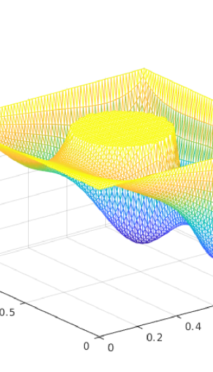
(a) The optimal control

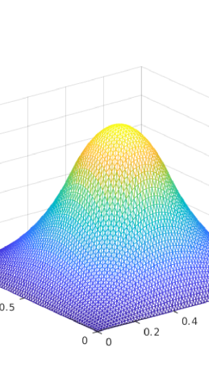
(b) The optimal state

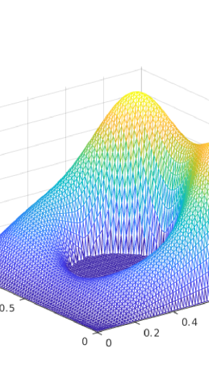
(c) The optimal adjoint state

(d) The multiplier $\displaystyle\mu$

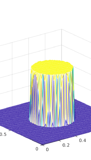
(e) The multiplier $\displaystyle\xi$

Figure 1: Example 1: The optimal control, state, adjoint state for $\displaystyle\gamma=10^{8}$.

Example 2 

This is Example 6.5 from [8] with lack of strict complementarity, where $\displaystyle f,y_{0}$ are replaced by $\displaystyle-f$ and $\displaystyle-y_{0}$. Here we choose for $\displaystyle(\mathbb{P})$ the data

$$\displaystyle\alpha=10^{-1},\quad y_{0}(x)=-(5x_{1}+x_{2}-1)\mbox{ in }\Omega,\quad f(x)=-(x_{1}-\frac{1}{2})\mbox{ in }\Omega,\quad\psi(x)=0\mbox{ in }\Omega.$$

We have

$$\alpha\lambda_{1}+\sqrt{\alpha^{2}\lambda^{2}_{1}+\alpha}\approx 3.9730.$$

The numerical results are reported in Table 2. We see that the condition (2.8) is satisfied for the considered values of $\displaystyle\gamma$, and hence, the unique global solution has been computed, which is presented in Figure 2 for $\displaystyle\gamma=10^{8}$. We again observe that the violation of the obstacle constraint satisfies $\displaystyle\min_{k\in\mathcal{N}^{-}}(y_{k}-\psi_{k})\sim-\gamma^{-1}$. This is also true in the subsequent examples.

Table 2: Example 2 where $\displaystyle\alpha\lambda_{1}+\sqrt{\alpha^{2}\lambda^{2}_{1}+\alpha}\approx 3.9730$.

$\displaystyle\gamma$	$\displaystyle\min_{k\in\mathcal{N}^{+}}\frac{p_{k}}{y_{k}-\psi_{k}}$	$\displaystyle\min_{k\in\mathcal{N}^{-}}\frac{3p_{k}}{\psi_{k}-y_{k}}$	$\displaystyle\eta$	$\displaystyle\min_{k\in\mathcal{N}^{-}}(y_{k}-\psi_{k})$	$\displaystyle\#N$
1.0e+00	-9.18374766e-01	5.31348016e+00	-9.18374766e-01	-8.34645660e-02	4
1.0e+01	-9.72376118e-01	5.75321935e+00	-9.72376118e-01	-5.91117294e-02	6
1.0e+02	-1.01940110e+00	8.79601682e+00	-1.01940110e+00	-7.28493127e-03	11
1.0e+03	-1.02120448e+00	9.45008887e+00	-1.02120448e+00	-7.34501977e-04	12
1.0e+04	-1.02054664e+00	8.61664669e+00	-1.02054664e+00	-7.65785826e-05	12
1.0e+05	-1.02044429e+00	8.29383499e+00	-1.02044429e+00	-7.76577329e-06	13
1.0e+06	-1.02030934e+00	8.19782461e+00	-1.02030934e+00	-7.83603514e-07	15
1.0e+07	-1.02028019e+00	8.13627555e+00	-1.02028019e+00	-7.85170648e-08	13
1.0e+08	-1.02027779e+00	8.12975658e+00	-1.02027779e+00	-7.85327708e-09	11
1.0e+09	-1.02027759e+00	8.12910469e+00	-1.02027759e+00	-7.85343418e-10	11
1.0e+10	-1.02027757e+00	8.12903950e+00	-1.02027757e+00	-7.85344989e-11	10
1.0e+11	-1.02027757e+00	8.12903298e+00	-1.02027757e+00	-7.85345146e-12	10
1.0e+12	-1.02027757e+00	8.12903233e+00	-1.02027757e+00	-7.85345161e-13	10

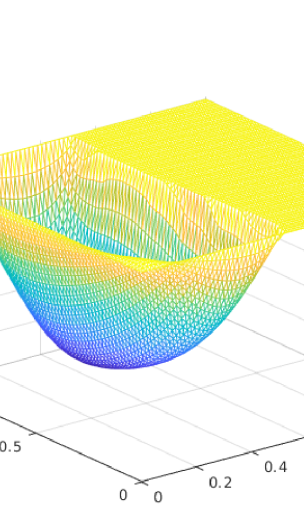
(a) The optimal control

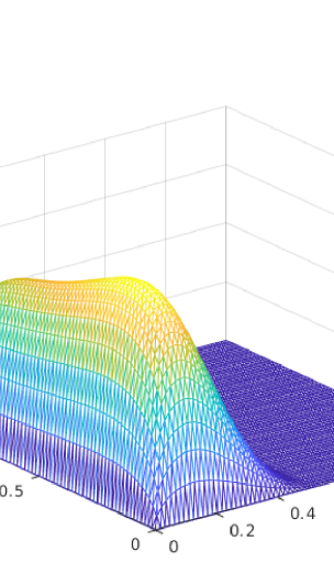
(b) The optimal state

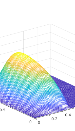
(c) The optimal adjoint state

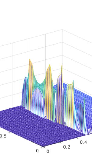
(d) The multiplier $\displaystyle\mu$

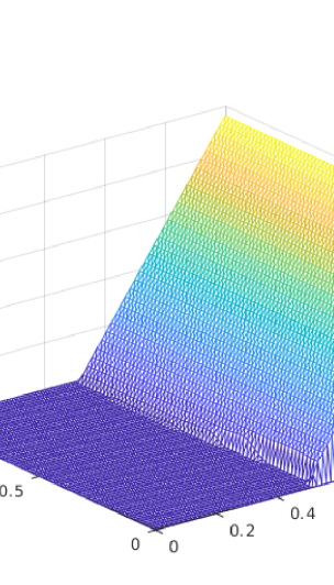
(e) The multiplier $\displaystyle\xi$

Figure 2: Example 2: The optimal control, state and adjoint state for $\displaystyle\gamma=10^{8}$.

Example 3 

The data of this Example 1 is taken from [11], where an exact solution for $\displaystyle(\mathbb{P})$ is constructed as follows;

$$\displaystyle\alpha=1,\quad\psi=0\mbox{ in }\Omega,$$

$$\displaystyle f(x)=-\Delta y(x)-\xi(x)+\frac{1}{\alpha}p(x)\mbox{ in }\Omega$$

$$\displaystyle y_{0}(x)=\begin{cases}y(x)+\Delta p_{1}(Q^{t}x)&\quad\text{ in }\Omega_{1},\\ y(x)&\quad\text{otherwise}.\end{cases}$$

Here $\displaystyle y$ denotes the optimal state with the corresponding adjoint state $\displaystyle p$ and slackness variable $\displaystyle\xi$, which are defined by

$$\displaystyle y(x_{1},x_{2}) \displaystyle=\begin{cases}y_{1}(x_{1})\cdot y_{2}(x_{2})&\quad\text{ in }(0,0.5)\times(0,0.8),\\ 0&\quad\text{otherwise},\end{cases}$$

$$\displaystyle p(x) \displaystyle=\begin{cases}p_{1}(Q^{t}x)&\quad\text{ in }\Omega_{1},\\ 0&\quad\text{otherwise},\end{cases}$$

$$\displaystyle\xi(x_{1},x_{2}) \displaystyle=\begin{cases}y_{1}(x_{1}-0.5)\cdot y_{2}(x_{2})&\quad\text{ in }(0.5,1)\times(0,0.8),\\ 0&\quad\text{otherwise}.\end{cases}$$

Moreover, $\displaystyle y_{1}$, $\displaystyle y_{2}$, and $\displaystyle p_{1}$ are the functions

$$\displaystyle y_{1}(x_{1})=-4096x_{1}^{6}+6144x_{1}^{5}-3072x_{1}^{4}+512x_{1}^{3},$$

$$\displaystyle y_{2}(x_{2})=-244.140625x_{2}^{6}+585.9375x_{2}^{5}-468.75x_{2}^{4}+125x_{2}^{3},$$

$$\displaystyle p_{1}(x_{1},x_{2})=(-200(x_{1}-0.8)^{2}+0.5)(-200(x_{2}-0.9)^{2}+0.5),$$

and $\displaystyle\Omega_{1}$ is the square with midpoint (0.8,0.9) and edge length 0.1 after being rotated by the matrix

$$Q=\begin{bmatrix}\cos\frac{\pi}{6}&-\sin\frac{\pi}{6}\\ \sin\frac{\pi}{6}&\cos\frac{\pi}{6}\end{bmatrix}$$

around its midpoint. This example contains the biactive set

$$\{x\in\Omega;y(x)=\xi(x)=0\}\equiv[0,1]\times[0.8,1],$$

which makes its numerical treatment challenging. Furthermore should we note that in this example the cost functional is of the form

$$J(y,u)=\frac{1}{2}\|y-y_{0}\|_{L^{2}(\Omega)}^{2}+\frac{1}{2}\|u-u_{d}\|_{L^{2}(\Omega)}^{2}$$

with $\displaystyle u_{d}=u+\frac{1}{\alpha}p$. We account for $\displaystyle u_{d}$ in the setting of $\displaystyle f$ above. Our theory also is valid in this situation without further modifications, see the proof of Lemma 2.1.

From the previous data we have

$$\alpha\lambda_{1}+\sqrt{\alpha^{2}\lambda^{2}_{1}+\alpha}\approx 39.5037.$$

We provide the numerical results in Table 3. Again, the unique global minimum has been computed and the corresponding graphs are illustrated in Figure 3 when $\displaystyle\gamma=10^{8}$.

Table 3: Example 3 with $\displaystyle\alpha\lambda_{1}+\sqrt{\alpha^{2}\lambda^{2}_{1}+\alpha}\approx 39.5037$

. $\displaystyle\gamma$ $\displaystyle\min_{k\in\mathcal{N}^{+}}\frac{p_{k}}{y_{k}-\psi_{k}}$ $\displaystyle\min_{k\in\mathcal{N}^{-}}\frac{3p_{k}}{\psi_{k}-y_{k}}$ $\displaystyle\eta$ $\displaystyle\min_{k\in\mathcal{N}^{-}}(y_{k}-\psi_{k})$ $\displaystyle\#N$ 1.0e+00 1.63643751e-02 3.74767766e+00 0.00000000e+00 -2.10533852e-02 3 1.0e+01 1.58450462e-02 3.61352870e+00 0.00000000e+00 -2.07865748e-02 4 1.0e+02 1.97319240e-03 1.04106448e-01 0.00000000e+00 -8.25007721e-03 8 1.0e+03 -1.25202529e-02 -3.51210686e-01 -3.51210686e-01 -9.83097618e-04 11 1.0e+04 -2.42618027e-01 -3.37078927e-01 -3.37078927e-01 -9.97061633e-05 12 1.0e+05 -1.36127707e-01 -1.12485742e-01 -1.36127707e-01 -1.02473476e-05 13 1.0e+06 -9.75060053e-02 -3.06984382e-02 -9.75060053e-02 -1.03346212e-06 15 1.0e+07 -8.26915590e-02 -3.18139489e-02 -8.26915590e-02 -1.03449193e-07 13 1.0e+08 -1.81555278e-01 -3.47707710e-02 -1.81555278e-01 -1.03459974e-08 14 1.0e+09 -2.20032200e-01 -4.44457854e-02 -2.20032200e-01 -1.03461058e-09 15 1.0e+10 -2.24336956e-01 -4.55306972e-02 -2.24336956e-01 -1.03461166e-10 17 1.0e+11 -2.24772813e-01 -4.56405644e-02 -2.24772813e-01 -1.03461177e-11 16

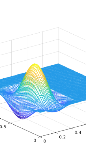
(a) The optimal control

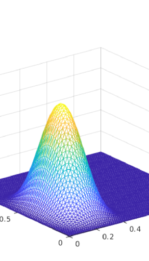
(b) The optimal state

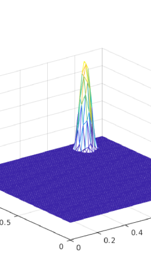
(c) The optimal adjoint state

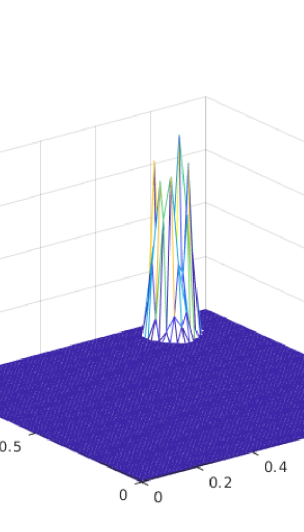
(d) The multiplier $\displaystyle\mu$

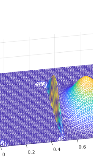
(e) The multiplier $\displaystyle\xi$

Figure 3: Example 3: The optimal control, state, adjoint state, and the multipliers for $\displaystyle\gamma=10^{8}$.

Example 4 

The data for this problem is taken from Example 6.2 in [12] and for $\displaystyle(\mathbb{P})$ reads

$$\displaystyle\alpha=1,\quad\psi(x)=0\mbox{ in }\Omega,\quad f(x)=\frac{1}{2}+\frac{1}{2}(x_{1}-x_{2})\mbox{ in }\Omega,$$

$$\displaystyle y_{0}(x)=\begin{cases}-1\quad\text{ if }|x|\geq 0.1,\\ 1-100x_{1}^{2}-50x_{2}^{2}\quad\text{otherwise}.\end{cases}$$

We have

$$\alpha\lambda_{1}+\sqrt{\alpha^{2}\lambda^{2}_{1}+\alpha}\approx 19.3313.$$

The numerical results are reported in Table 4. The condition (2.8) is satisfied, and hence, the unique global solution has been computed, which we illustrate in Figure 4 for $\displaystyle\gamma=10^{8}$.

Table 4: Example 4 where $\displaystyle\alpha\lambda_{1}+\sqrt{\alpha^{2}\lambda^{2}_{1}+\alpha}\approx 19.3313$.

$\displaystyle\gamma$	$\displaystyle\min_{k\in\mathcal{N}^{+}}\frac{p_{k}}{y_{k}-\psi_{k}}$	$\displaystyle\min_{k\in\mathcal{N}^{-}}\frac{3p_{k}}{\psi_{k}-y_{k}}$	$\displaystyle\eta$	$\displaystyle\min_{k\in\mathcal{N}^{-}}(y_{k}-\psi_{k})$	$\displaystyle\#N$
1.0e+00	1.28191544e+00	9.12899685e+00	0.00000000e+00	-7.61042379e-03	3
1.0e+01	1.28189321e+00	9.11848759e+00	0.00000000e+00	-7.59555549e-03	3
1.0e+02	1.27854041e+00	7.14870263e+00	0.00000000e+00	-4.77178798e-03	7
1.0e+03	1.27598179e+00	2.95273878e+00	0.00000000e+00	-7.05858478e-04	11
1.0e+04	1.27568823e+00	2.30861182e+00	0.00000000e+00	-7.60379296e-05	12
1.0e+05	1.27561164e+00	2.14128368e+00	0.00000000e+00	-7.76063518e-06	12
1.0e+06	1.27562640e+00	2.08304474e+00	0.00000000e+00	-7.81857173e-07	13
1.0e+07	1.27563830e+00	2.06636877e+00	0.00000000e+00	-7.84995677e-08	15
1.0e+08	1.27563972e+00	2.06470139e+00	0.00000000e+00	-7.85310208e-09	11
1.0e+09	1.27563987e+00	2.06453466e+00	0.00000000e+00	-7.85341667e-10	11
1.0e+10	1.27563988e+00	2.06451798e+00	0.00000000e+00	-7.85344814e-11	10
1.0e+11	1.27563988e+00	2.06451631e+00	0.00000000e+00	-7.85345128e-12	10
1.0e+12	1.27563989e+00	2.06451615e+00	0.00000000e+00	-7.85345160e-13	10

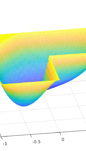
(a) The optimal control

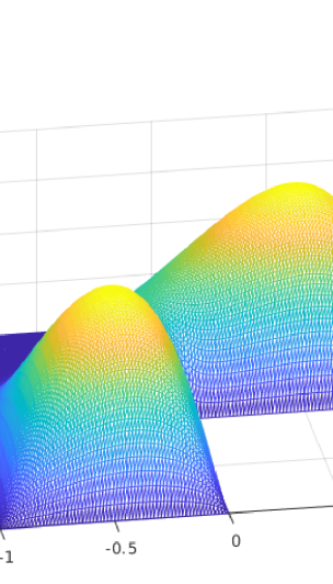
(b) The optimal state

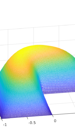
(c) The optimal adjoint state

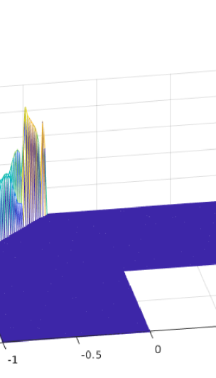
(d) The multiplier $\displaystyle\mu$

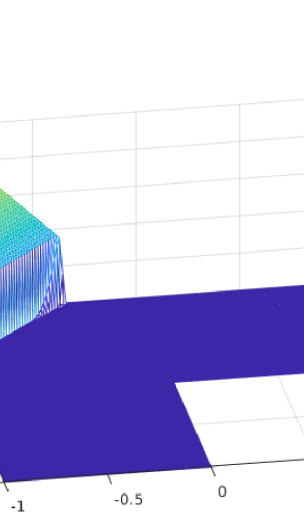
(e) The multiplier $\displaystyle\xi$

Figure 4: Example 4: The optimal control, state, adjoint state, and the multipliers for $\displaystyle\gamma=10^{8}$.

References

- [1] A. Ahmad Ali, K. Deckelnick and M. Hinze, Global minima for semilinear optimal control problems. Comput. Optim. Appl. 65, 261–288 (2016).
- [2] A. Ahmad Ali, K. Deckelnick and M. Hinze, Error analysis for global minima of semilinear optimal control problems. Mathematical Control and related Fields 8, 195–215 (2018).
- [3] V. Barbu, Optimal control of variational inequalities. Res. Notes Math. 100, Pitman, Boston, 1984.
- [4] S. Bartels, Numerical methods for nonlinear partial differential equations. Springer Series in Computational Mathematics, 47. Springer, Cham, 2015.
- [5] M. Bergounioux and F. Mignot, Optimal control of obstacle problems: existence of Lagrange multipliers. ESAIM Control Optim. Calc. Var. 5, 45–70 (2000).
- [6] M. Hintermüller, Inverse coefficient problems for variational inequalities: Optimality conditions and numerical realization. ESAIM Math. Model. Numer. Anal. 35, 129–152 (2001).
- [7] M. Hintermüller and I. Kopacka, A smooth penalty approach and a nonlinear multigrid algorithm for elliptic MPECs. Comput. Optim. Appl. 50, 111–145 (2011).
- [8] K. Ito and K. Kunisch, Optimal control of elliptic variational inequalities. Appl. Math. Optim. 41, 343–364 (2000).
- [9] K. Kunisch and D. Wachsmuth, Path–following for optimal control of stationary variational inequalities. Comput. Opt. Appl. 51, 1345–1373 (2012).
- [10] K. Kunisch and D. Wachsmuth, Sufficient optimality conditions and semi–smooth Newton methods for optimal control of stationary variational inequalities. ESAIM Control Optim. Calc. Var. 18, no. 2, 520–-547 (2012).
- [11] C. Meyer and O. Thoma, A priori finite element error analysis for optimal control of the obstacle problem. SIAM J. Numer. Anal. 51, 605–628 (2013).
- [12] C. Meyer, A. Rademacher, and W. Wollner, Adaptive optimal control of the obstacle problem. SIAM J. Sci. Comput. 37, 918–945 (2015).
- [13] F. Mignot, Contrôle dans les inéquations variationelles elliptiques. J. Funct. Anal. 22, 130–185 (1976).
- [14] F. Mignot and J.-P. Puel, Optimal control in some variational inequalities. SIAM J. Control Optim. 22 (3), 466–476 (1984).
- [15] A. Schiela and D. Wachsmuth, Convergence analysis of smoothing methods for optimal control of stationary variational inequalities with control constraints. ESAIM Math. Model. Numer. Anal. 47, no. 3, 771–787 (2013).
- [16] G. Wachsmuth, Strong stationarity for optimal control of the obstacle problem with control constraints. SIAM J. Optim. 24 (1), 1914–1932 (2014).