CONVOLUTIONAL GROUP-SPARSE CODING AND SOURCE LOCALIZATION

Abstract

In this paper, we present a new interpretation of non-negatively constrained convolutional coding problems as blind deconvolution problems with spatially variant point spread function. In this light, we propose an optimization framework that generalizes our previous work on non-negative group sparsity for convolutional models. We then link these concepts to source localization problems that arise in scientific imaging, and provide a visual example on an image derived from data captured by the Hubble telescope.

Index Terms—  Sparse representation, Source localization, Non-negative group sparsity

1 Introduction

Convolutional sparse representations, or convolutional sparse coding (CSC), have been the subject of study of many recent publications in the deep learning and signal processing communities, see, for example, [1] and the references therein. CSC has been used for feature extraction in biological imaging [2], musical representation and transcription [3, 4], and pedestrian detection [5], among others. The fundamental advantage of CSC over previous sparse representations is that it naturally allows for invariance constraints to be part of the feature extraction process, e.g. [6, 1]. Besides imposing desired properties on the extracted features, these invariance constraints greatly reduce the number of model parameters, and thereby, training complexity.

In this paper, we shift the paradigm from feature extraction towards generative models and inverse problems. In fact, we interpret convolutional coding as a means of relaxing the invariance constraints of a simple convolutional model. A known approach to blind deconvolution with a spatially variant (SV) point spread function (PSF) is approximating the SV kernel as a spatially weighted combination of elements of a low-dimensional kernel basis [7]. In this paper, we show that a non-negatively constrained version of the optimization problem used for convolutional coding can be interpreted in this manner, placing CSC in the context of a longstanding open problem with many recent contributions [8, 9, 7, 10, 11]. With this new framework in mind, we propose to replace the sparsity regularizer in the convolutional basis pursuit denoising problem [1] by a non-negative group-sparsity regularizer [12], and call the resulting technique convolutional group-sparse coding (CGSC). This novel technique generalizes our proposal in [13, 14], and can be applied to a number of settings by using different groupings of the variables involved.

For example, in diverse scientific scenarios, image data can be explained in terms of a number of point- or extended-sources emitting some measurable signal (see Fig. 1 for two example images), e.g. [15, 16, 17, 18, 19, 20, 13, 14], and source localization (SL) methods automate the accurate localization of these sources. In [13, 14], we derived and analyzed a physically-motivated generative model for ELISPOT and Fluorospot biomedical images. This led us to an optimization problem formulation for SL on these images that naturally included a fixed convolutional dictionary and non-negativity constraints on the feature maps. In this paper, we generalize that formulation to fit generic SL problems, and present a visual example with a composite image obtained from data captured by one of the wide field cameras in the Hubble telescope.

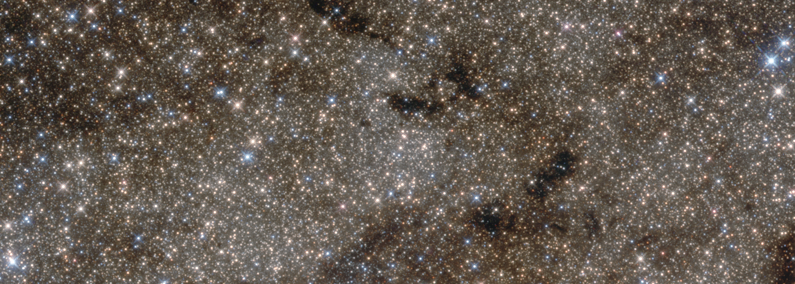
(a) Section of an image of the Milky Way’s nuclear star cluster

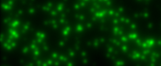
(b) Section of a synthetic Fluorospot observation

Fig. 1: Scientific imaging examples in which source localization (SL) is needed. Above, section of a composite color image of the Milky Way’s nuclear star cluster, generated by The Hubble Heritage Team, NASA and ESA (STScI-2016-11) from an image capture using Hubble’s Wide Field Camera 3. Below, a section of a synthetic Fluorospot image observation, generated using our results in [14].

2 Convolutional Group-Sparse Coding

2.1 Convolutional coding

In convolutional coding, one models an image observation $s\in\operatorname{\mathbb{T}}\left(M,N\right)$ as

$$s=\sum_{k=1}^{K}h_{k}\circledast x_{k}+n\,,$$ (1)

where $n\in\operatorname{\mathbb{T}}\left(M,N\right)$ is additive noise, $\{x_{k}\}_{1}^{K}\subset\operatorname{\mathbb{T}_{+}}\left(M,N\right)$ are $K$ different images or feature maps, and $\{h_{k}\}_{1}^{K}$ is some dictionary of convolutional kernels. Here, $\operatorname{\mathbb{T}}\left(\mathcal{S},Q_{1},Q_{2}\right)$ are the matrices of dimension $Q_{1}\times Q_{2}$ with elements in the one-dimensional set $\mathcal{S}$, $\operatorname{\mathbb{T}}\left(\mathbb{R},Q_{1},Q_{2}\right)$ is shortened as $\operatorname{\mathbb{T}}\left(Q_{1},Q_{2}\right)$, and $\operatorname{\mathbb{T}}\left(\mathbb{R}_{+},Q_{1},Q_{2}\right)$ as $\operatorname{\mathbb{T}_{+}}\left(Q_{1},Q_{2}\right)$. Furthermore, $\circledast$ represents a zero-padded, same-size discrete convolution. For the model in (1), one aims to find the most adequate $x_{k}$s (according to some criteria) to explain $s$, for some specific collection of $h_{k}$s. The non-negativity constraint $x_{k}\in\operatorname{\mathbb{T}_{+}}\left(M,N\right)$ is not standard in the literature, but does not restrict use either. Indeed, one can incorporate pairs $\{h,-h\}$ to $\{h_{k}\}_{1}^{K}$ to obtain the usual model. Our focus here, however, will be in preserving these non-negativity constraints on the feature maps.

In CSC, the model-fit is generally performed using the convolutional basis pursuit denoising problem [1], which, after the inclusion of the aforementioned non-negativity constraints, is of the form

$$\min_{\{x_{k}\in\operatorname{\mathbb{T}_{+}}\left(M,N\right)\}_{1}^{K}}\left\{\left\|\sum_{k=1}^{K}h_{k}\circledast x_{k}-s\right\|_{2}^{2}+\lambda\sum_{k=1}^{K}\left\|x_{k}\right\|_{1}\right\}\,.$$ (2)

Non-negativity gains importance when we define the new variables $y\in\operatorname{\mathbb{T}_{+}}\left(M,N\right)$ and $\alpha_{k}\in\operatorname{\mathbb{T}}\left([0,1],M,N\right)$ for $k\in\{1,2,\dots,K\}$ such that

$$y=\sum_{k=1}^{K}x_{k},\mbox{ and }\alpha_{k}[i,j]=\frac{x_{k}[i,j]}{y[i,j]}\mbox{ if }y[i,j]>0\,,$$

that allow us to rewrite the model in (1) as

$$s[\tilde{i},\tilde{j}]=\sum_{i,j}y[i,j]\sum_{k=1}^{K}\alpha_{k}[i,j]h_{k}[\tilde{i}-i,\tilde{j}-j].$$ (3)

Here, for a specific pixel position $(i,j)$, the $\alpha_{k}[i,j]$s are convex combination coefficients that express the PSF at location $(i,j)$ with respect to the basis $\{h_{k}\}_{1}^{K}$. Therefore, (3) reveals that solving (2) is equivalent to performing least-squares recovery of a sparse image $y$ that has been blurred by a SV PSF restricted to the convex hull of $\{h_{k}\}_{1}^{K}$.

As it is common in CSC [1], we will further on consider a norm constraint on the $h_{k}$s to avoid the scaling ambiguity between filters and coefficients. In contrast to [1, Section V], that imposes $\left\|h_{k}\right\|_{2}=1$, we will impose the $h_{k}$s to have the same $1$-norm $\left\|h_{k}\right\|_{1}$. The model in (3) reveals that this is more convenient, because it corresponds to simply assuming that the local PSF has constant $1$-norm throughout the image.

2.2 Convolutional group-sparse coding

The model in (3) suggests that the relation between the $x_{k}[i,j]$s in (2) could be further exploited. For example, one may accept that in some area the local PSF is described as a convex combination of $h_{1}$ and $h_{2}$, but it may well be the case that in some other area the combination of these two kernels is unlikely. In other words, previous knowledge could be incorporated by locally forcing a model selection between unlikely combinations and joint or group behavior between likely combinations. To this end, we propose to define $G$ sets $\left\{\mathcal{G}_{g}\right\}_{1}^{G}$ of indices $(i,j,k)$ such that $\mathcal{G}_{g_{1}}\cap\mathcal{G}_{g_{2}}=\emptyset$ for $g_{1}\neq g_{2}$, and solve the following least-squares, non-negative group-sparsity regularized problem instead,

$$\min_{\{x_{k}\}_{1}^{K}}\!\left\{\left\|\sum_{k=1}^{K}h_{k}\circledast x_{k}-s\right\|_{w}^{2}\!\!\!\!+\!\lambda\sum_{g=1}^{G}\sqrt{\sum_{(i,j,k)\in\mathcal{G}_{g}}\!\!\!\!\!x_{k}^{2}[i,j]}\right\}\,,$$ (4)

with $x_{k}\in\operatorname{\mathbb{T}_{+}}\left(M,N\right)$ for every $k$. Here, we use the norm $\|\cdot\|_{w}=\|w\odot\cdot\|_{2}$ (where $\odot$ stands for the Hadamard product) to allow for a non-negative weighting $w\in\operatorname{\mathbb{T}_{+}}\left(M,N\right)$ that judges differently prediction errors at different locations. This new problem formulation (4), which we name convolutional group-sparse coding (CGSC), will induce a group behavior [12] on the elements $x_{k}[i,j]$ such that $(i,j,k)$ belong to the same $\mathcal{G}_{g}$. Note that (4) is a convex problem, and that it includes (2) as a specific case, in which one chooses $M\times N\times K$ groups of a single index vector.

Group sparsity regularization for convolutional coding has been used previously in the context of multimodal imaging [21, 22], in which grouping promoted the fusion of information from different imaging sensors or modalities. However, these approaches do not consider non-negativity of the feature maps, which plays an fundamental role in SL and in the interpretation of CSC as a deconvolution with SV kernels.

2.3 Accelerated proximal gradient algorithm

 

0:   $\{x_{k}^{(0)}\}_{1}^{K}\subset\operatorname{\mathbb{T}_{+}}\left(M,N\right)$, an image $s\in\operatorname{\mathbb{T}}\left(M,N\right)$, a weight $w\in\operatorname{\mathbb{T}_{+}}\left(M,N\right)$ and a kernel dictionary $\left\{h_{k}\right\}_{1}^{K}$  

0:  

1:  $l\leftarrow 0$

2:  for  $k=1$ to $K$ do

3:     $\displaystyle z_{k}^{(0)}\leftarrow x_{k}^{(0)}$,

4:  end for

5:  repeat

6:     $l\leftarrow l+1$

7:     $\displaystyle u^{(l)}\leftarrow\sum_{k=1}^{K}h_{k}\circledast z^{(l-1)}_{k}-s$

8:     for  $k=1$ to $K$ do

9:        $\displaystyle x_{k}^{(l)}\leftarrow\left[z_{k}^{(l-1)}-h^{\mathrm{m}}_{k}\circledast\left[w\odot u^{(l)}\right]\right]_{+}$

10:     end for

11:     for  $g=1$ to $G$ do

12:        $\displaystyle n\leftarrow\sqrt{\sum_{(i,j,k)\in\mathcal{G}_{g}}\left(x^{(l)}_{k}[i,j]\right)^{2}}$

13:        for  $(i,j,k)\in\mathcal{G}_{g}$ do

14:           $\displaystyle x^{(l)}_{k}[i,j]\leftarrow\left(1-\frac{\lambda}{2}n^{-1}\right)_{+}x^{(l)}_{k}[i,j]$

15:        end for

16:     end for

17:     for  $k=1$ to $K$ do

18:        $z_{k}^{(l)}\leftarrow x_{k}^{(l)}+\alpha(l)\left(x_{k}^{(l)}-x_{k}^{(l-1)}\right)$

19:     end for

20:  until  convergence of $\{x_{k}^{(l)}\}_{1}^{K}$

20:    

Fig. 2: APG algorithm for CGSC, solving (4). The sequence $\alpha(l)$ can be that in [23] or that in [24].

Proximal optimization algorithms have been widely used for CSC [25, 4, 26, 27, 1]. In [13], we derived the accelerated proximal gradient (APG) algorithm (also known as FISTA) to solve a functional optimization problem closely related to (4). Here, we will derive the APG algorithm to solve (4), reported in Fig. 2, often referring to our previous results in [13].

To obtain the APG algorithm for (4), one needs to characterize the mapping $\{x_{k}\}_{1}^{K}\mapsto\sum_{k=1}^{K}h_{k}\circledast x_{k}$ in terms of A) its adjoint and B) an upper bound on its operator norm (see [13, Section IV-B]). With respect to A), while in [13] we relied on the self-adjointness of convolutional operators with symmetric kernel, here we have not imposed any symmetry restrictions on the $h_{k}$s. Nonetheless, following [13, Appendix A, Proofs - Property 3 and Lemma 2], it is clear that the adjoint we seek is the mapping $u\mapsto\left\{h^{\mathrm{m}}_{k}\circledast\left[w\odot u\right]\right\}_{1}^{K}$, where the $h^{\mathrm{m}}_{k}$s are the matched filters corresponding to the $h_{k}$s, constructed by inverting the order of the elements in the kernel matrix in both dimensions. This result was implicitly stated before in [25] in its derivation of the FISTA for CSC. With respect to B), in [13] we used that Gaussian functions have unit $1$-norm. As mentioned in Section 2.1, and to simplify the expressions in the final algorithm, we assume that $\left\|h_{k}\right\|_{1}=K^{-1}\|w\|^{-2}_{\infty}$, which, following [13, Appendix A, Proof - Lemma 1], provides that the operator norm of the aforementioned mapping is bounded above by $1$.

Furthermore, one needs to obtain the proximal operator [28] corresponding to the non-negative group-sparsity regularizer in (4). In [13, Appendix B - Lemma 6], we provided the proximal operator of the non-negative $2$-norm in some space. The proofs there generalize well to each partition of $\operatorname{\mathbb{T}}\left(M,N,K\right)$ established by the index groups $\{\mathcal{G}_{g}\}_{1}^{G}$. Combining those results with the separable sum property [29], we obtain that if $\{z_{k}\}_{1}^{K}$ are the result of evaluating the proximal operator of the non-negative group-sparsity regularizer at $\{x_{k}\}_{1}^{K}$, then $z_{k}[i,j]=Q_{+}[i,j,k]\left(x_{k}[i,j]\right)_{+}$ with

$$Q_{+}[i,j,k]=\left(1-\frac{\lambda}{2}\left[\sqrt{\sum_{(i,j,k)\in\mathcal{G}_{g}}\left(\left[x_{k}[i,j]\right]_{+}\right)^{2}}\right]^{-1}\right)_{+},$$

if $(i,j,k)\in\mathcal{G}_{g}$ and $Q=1$ if $(i,j,k)$ does not belong to any of the $\mathcal{G}_{g}$s. As expected, this result has the structure of a block soft thresholding operator [29], but with the addendum of the projection onto the non-negative half-space.

These results are reflected in the algorithm in Fig. 2. In particular, Lines 7 and 9 implement the gradient step with adequate step-size and non-negative projection, and Lines 12 and 14 implement the proximal operator of the non-negative group-sparsity regularizer.

3 CGSC for source localization

In many cases, image-based SL problems are characterized by noisy images with bright spots of different shapes and sizes that often occlude each other. Each of these spots represents a relevant source, and thus, the objective of the problem is to accurately distinguish and locate each of the spots. Example applications are the localization and counting of stars in astronomy and cells in biology, e.g. Fig. 1.

These problems can be addressed in terms of a blind deconvolution problem with SV PSF. With respect to the notation in (3), the underlying image $y$ is a detailed geographical map of the sources that characterizes them in terms of their location and brightness, while the shapes and sizes of each of the spots are expressed in terms of a convex combination of kernels in the dictionary $\{h_{k}\}$. In this context, then, we propose the APG algorithm for CGSC in Fig 2, with $G=M\times N\times P$ groups of the shape

$$\mathcal{G}_{i,j,p}=\left\{(m,n,k):m=i,n=j,k\in\aleph_{p}\right\}\,,$$ (5)

with $p\in\{1,2,\dots,P\}$.

In (5), the $\aleph_{p}$s are sets of $k$s that express which kernels $h_{k}$ should be considered for use jointly to express a spot shape. If $\{1,2,\dots,K\}\setminus\cup_{p=1}^{P}\aleph_{p}\neq\emptyset$, those $k$s correspond to kernels that are used to account for background patterns or other artifacts that are not to be considered sources. This choice corresponds to a grouping effect for all those terms representing a single location that should be considered jointly, placing the focus on determining whether or not a specific spatial location held a source. Note that the application of CGSC to SL is only possible due to the non-negativity constraints in (4), as the otherwise unconstrained optimization proble would also try to predict dark shapes in terms of the corresponding negative kernels $\{-h_{k}\}_{1}^{K}$. The formulation for SL composed by (4) and (5) generalizes our proposed approach in [13, 14] for cell detection in ELISPOT and Fluorospot data. An application example is provided in Section 4 using the image section from the Hubble telescope (see Fig 1).

The challenge of choosing the base $\{h_{k}\}_{1}^{K}$ to successfully approximate spot shapes and background patterns remains. On one hand, data-based solutions to this problem, i.e. convolutional dictionary learning, have been extensively discussed in the literature, e.g., [1, Section II-D] and references therein. On the other hand, in [13, 14], we analyzed the physical model for ELISPOT and Fluorospot assays, and derived an observation model for the resulting images. Discretizing this observation model lead us to an expression for the image observation of the form in (1), where exact expressions for the $h_{k}$s were known, and the only source of error was discretization in itself. Finally, a first approximate solution can be obtained for new applications by choosing an initial base $\{h_{k}\}_{1}^{K}$ based on heuristic reasoning and refining it by trial-and-error.

4 Experimental results

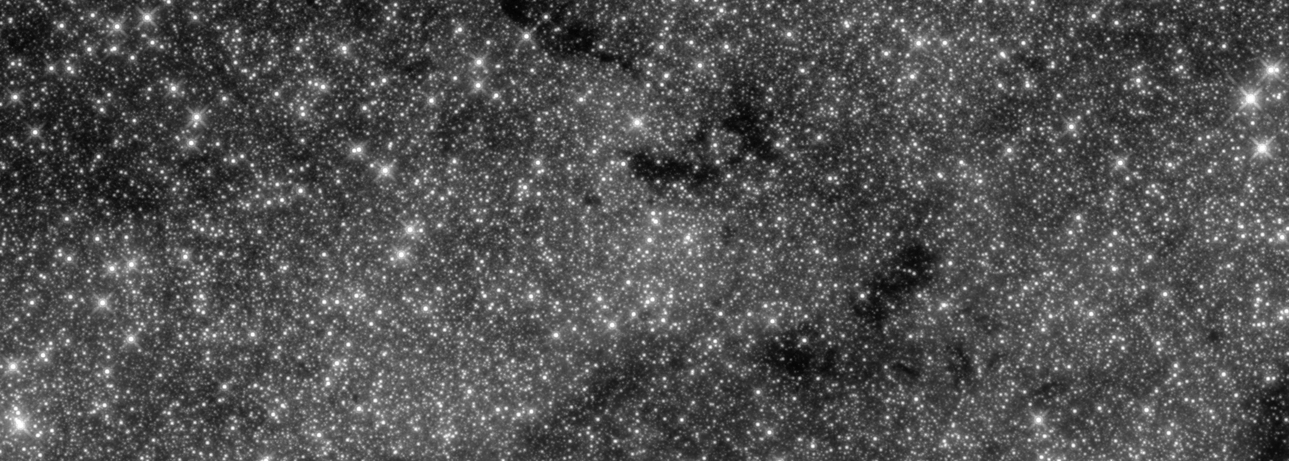
(a) Section of an image of the Milky Way’s nuclear star cluster

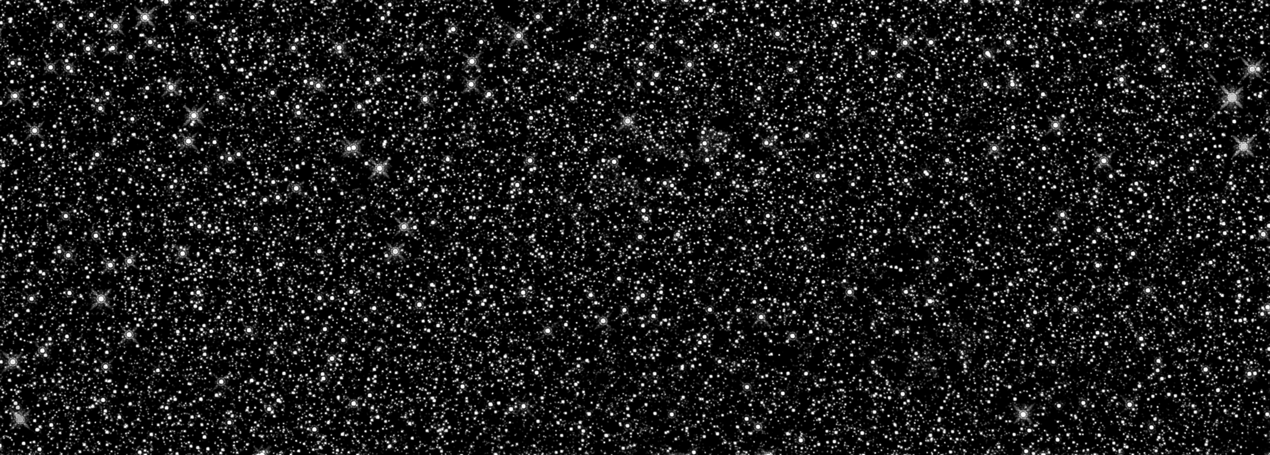
(b) Recovery of the foreground component using CGSC

(c) Battery of filters $\{h_{k}\}_{1}^{K}$, $k$ increasing from left to right.

Fig. 3: Foreground reconstruction using the APG algorithm for CGSC in Fig. 2. Above, grayscale image. Middle, foreground recovery, artificially saturated for printing clarity, showing only lower half of dynamic range. Below, set of filters used for foreground (left to right, first $5$ filters) and background prediction (last filter).

In our previous works [13, 14], we provided extensive quantitative validation of a restricted version of the algorithm in Fig. 2 for cell detection on ELISPOT and Fluorospot data, both with synthetic images and real, expertly-labeled images. Here, we present a qualitative example from an entirely different setting, using the more general formulation in (4). The image in the upper part of Fig. 1 is a section of a composite image of the Milky Way’s nuclear star cluster, generated as part of a study to determine the structure and origin of this cluster (STScI-2016-11). The study aimed to recover the cluster’s total mass and its dynamic behavior. For both these purposes, an accurate localization and count of the stars from this and similar images was important. Besides the massive amount of stars, part of the problem in this task was the background variations caused by dense dust clouds that surrounded the relevant stars and absorbed part their infrared emissions.

In Fig. 3, we report the results of a first approximation to the problem using $1000$ iterations of the APG algorithm for CGSC in Fig. 2, with $\lambda=0.01$, $w=1$ everywhere and $K=6$. In particular, we choose an heuristic set of $h_{k}$s, shown in Fig. 3(c), and use them to predict how the image, Fig. 3(a), would appear without a background component, i.e., Fig. 3(b). Of the filters in Fig. 3(c), the first is a middle-sized star with a complex shape extracted from the image itself, the second is an up-sampled (scale $4/3$) version of the same star, included to match larger stars, and the remaining four are spatially-integrated (within a pixel) rotationally-symmetric Gaussian kernels with different standard deviations included to match smaller stars (from left to right, $\sigma=1$, $\sigma=2$, $\sigma=5$) and background variations (last, $\sigma=50$). Consequently, with respect to the notation in Section 3, we choose $\aleph_{1}=\{1\}$, $\aleph_{2}=\{2\}$, $\aleph_{3}=\{3,4,5\}$. This implies that for each pixel, we consider three different groups of variables, the two first corresponding to the explanation of a spot by a simple copy of one of the two first kernels, and the third corresponding to the explanation of a spot by a convex combination of the shapes in the next three kernels. Finally, the variable that corresponds to the last kernel is not regularized. Therefore, if a pattern can be matched by the last, much wider kernel, that explanation will be preferred, and the pattern will be considered as part of the background.

Fig. 3(b) exhibits an impressive foreground reconstruction, at the low cost of a basic heuristic proposal for $\{h_{k}\}_{1}^{K}$ based only on the most obvious patterns in the image. Specialized insight on the physical modeling of star emissions and the patterns that arise in the Hubble’s telescope wide field cameras could, in our opinion, open the door to complete SL and counting in these images at the remarkable accuracy levels we obtained in [13, 14] for ELISPOT and Fluorospot data.

References

- [1] B. Wohlberg, “Efficient algorithms for convolutional sparse representations,” IEEE Transactions on Image Processing, vol. 25, no. 1, pp. 301–315, Jan. 2016.
- [2] Marius Pachitariu, Adam M Packer, Noah Pettit, Henry Dalgleish, Michael Hausser, and Maneesh Sahani, “Extracting regions of interest from biological images with convolutional sparse block coding,” in Advances in Neural Information Processing Systems 26, C. J. C. Burges, L. Bottou, M. Welling, Z. Ghahramani, and K. Q. Weinberger, Eds., pp. 1745–1753. Curran Associates, Inc., 2013.
- [3] T. Blumensath and M. Davies, “Sparse and shift-invariant representations of music,” IEEE Transactions on Audio, Speech, and Language Processing, vol. 14, no. 1, pp. 50–57, Jan. 2006.
- [4] A. Cogliati, Z. Duan, and B. Wohlberg, “Piano music transcription with fast convolutional sparse coding,” in 2015 IEEE 25th International Workshop on Machine Learning for Signal Processing (MLSP), Sept. 2015, pp. 1–6.
- [5] Pierre Sermanet, Koray Kavukcuoglu, Soumith Chintala, and Yann Lecun, “Pedestrian detection with unsupervised multi-stage feature learning,” in The IEEE Conference on Computer Vision and Pattern Recognition (CVPR), June 2013.
- [6] Q. Barthelemy, A. Larue, A. Mayoue, D. Mercier, and J. I. Mars, “Shift & 2D rotation invariant sparse coding for multivariate signals,” IEEE Transactions on Signal Processing, vol. 60, no. 4, pp. 1597–1611, Apr. 2012.
- [7] Paul Escande and Pierre Weiss, “Sparse wavelet representations of spatially varying blurring operators,” SIAM Journal on Imaging Sciences, vol. 8, no. 4, pp. 2976–3014, 2015.
- [8] M. E. Daube-Witherspoon and G. Muehllehner, “An iterative image space reconstruction algorthm suitable for volume ECT,” IEEE Transactions on Medical Imaging, vol. 5, no. 2, pp. 61–66, June 1986.
- [9] Ralf C. Flicker and François J. Rigaut, “Anisoplanatic deconvolution of adaptive optics images,” J. Opt. Soc. Am. A, vol. 22, no. 3, pp. 504–513, Mar. 2005.
- [10] Joo Dong Yun and Seungjoon Yang, “ADMM in Krylov subspace and its application to total variation restoration of spatially variant blur,” SIAM Journal on Imaging Sciences, vol. 10, no. 2, pp. 484–507, 2017.
- [11] Daniel O’Connor and Lieven Vandenberghe, “Total variation image deblurring with space-varying kernel,” Computational Optimization and Applications, vol. 67, no. 3, pp. 521–541, July 2017.
- [12] Ming Yuan and Yi Lin, “Model selection and estimation in regression with grouped variables,” Journal of the Royal Statistical Society: Series B (Statistical Methodology), vol. 68, no. 1, pp. 49–67, 2006.
- [13] Pol del Aguila Pla and Joakim Jaldén, “Cell detection by functional inverse diffusion and group sparsity – Part I: Theory,” arXiv, 2017, Available at: arXiv:1710.01604v1.
- [14] Pol del Aguila Pla and Joakim Jaldén, “Cell detection by functional inverse diffusion and group sparsity – Part II: Practice,” arXiv, 2017, Available at: arXiv:1710.01622v1.
- [15] Giovannelli, J.-F. and Coulais, A., “Positive deconvolution for superimposed extended source and point sources,” A&A, vol. 439, no. 1, pp. 401–412, 2005.
- [16] Jonathan A. Rebhahn, Courtney Bishop, Anagha A. Divekar, Katty Jiminez-Garcia, James J. Kobie, F. Eun-Hyung Lee, Genny M. Maupin, Jennifer E. Snyder-Cappione, Dietmar M. Zaiss, and Tim R. Mosmann, “Automated analysis of two- and three-color fluorescent ELISPOT (Fluorospot) assays for cytokine secretion,” Computer Methods and Programs in Biomedicine, vol. 92, no. 1, pp. 54–65, 2008.
- [17] Ihor Smal, Marco Loog, Wiro Niessen, and Erik Meijering, “Quantitative comparison of spot detection methods in fluorescence microscopy,” IEEE Transactions on Medical Imaging, vol. 29, no. 2, pp. 282–301, Feb. 2010.
- [18] H. Ayasso, T. Rodet, A. Abergel, and K. Dassas, “A gradient-like variational bayesian approach for joint image super-resolution and source separation, application to astrophysical map-making,” in 2013 IEEE International Conference on Acoustics, Speech and Signal Processing (ICASSP), May 2013, pp. 5830–5834.
- [19] A. Benfenati and V. Ruggiero, “Inexact Bregman iteration for deconvolution of superimposed extended and point sources,” Communications in Nonlinear Science and Numerical Simulation, vol. 20, no. 3, pp. 882–896, 2015.
- [20] R. Mourya, L. Denis, J. M. Becker, and E. Thiébaut, “A blind deblurring and image decomposition approach for astronomical image restoration,” in 2015 23rd European Signal Processing Conference (EUSIPCO), Aug. 2015, pp. 1636–1640.
- [21] B. Wohlberg, “Convolutional sparse representation of color images,” in 2016 IEEE Southwest Symposium on Image Analysis and Interpretation (SSIAI), Mar. 2016, pp. 57–60.
- [22] Kevin Degraux, Ulugbek S Kamilov, Petros T Boufounos, and Dehong Liu, “Online convolutional dictionary learning for multimodal imaging,” arXiv preprint arXiv:1706.04256, 2017.
- [23] Amir Beck and Marc Teboulle, “A fast iterative shrinkage-thresholding algorithm for linear inverse problems,” SIAM Journal on Imaging Sciences, vol. 2, no. 1, pp. 183–202, 2009.
- [24] Antonin Chambolle and Charles Dossal, “On the convergence of the iterates of the fast iterative shrinkage/thresholding algorithm,” Journal of Optimization Theory and Applications, vol. 166, no. 3, pp. 968–982, 2015.
- [25] R. Chalasani, J. C. Principe, and N. Ramakrishnan, “A fast proximal method for convolutional sparse coding,” in The 2013 International Joint Conference on Neural Networks (IJCNN), Aug. 2013, pp. 1–5.
- [26] Shuhang Gu, Wangmeng Zuo, Qi Xie, Deyu Meng, Xiangchu Feng, and Lei Zhang, “Convolutional sparse coding for image super-resolution,” in The IEEE International Conference on Computer Vision (ICCV), Dec. 2015.
- [27] Felix Heide, Wolfgang Heidrich, and Gordon Wetzstein, “Fast and flexible convolutional sparse coding,” in The IEEE Conference on Computer Vision and Pattern Recognition (CVPR), June 2015.
- [28] Heinz H. Bauschke and Patrick L. Combettes, Convex analysis and monotone operator theory in Hilbert spaces, chapter 27. Proximal minimization, pp. 399–413, Springer New York, 2011.
- [29] Neal Parikh and Stephen Boyd, “Proximal algorithms,” Foundations and Trends ® in Optimization, vol. 1, no. 3, pp. 127–239, 2014.