A similarity measure for second order properties of non-stationary functional time series with applications to clustering and testing

Abstract

Due to the surge of data storage techniques, the need for the development of appropriate techniques to identify patterns and to extract knowledge from the resulting enormous data sets, which can be viewed as collections of dependent functional data, is of increasing interest in many scientific areas. We develop a similarity measure for spectral density operators of a collection of functional time series, which is based on the aggregation of Hilbert-Schmidt differences of the individual time-varying spectral density operators. Under fairly general conditions, the asymptotic properties of the corresponding estimator are derived and asymptotic normality is established. The introduced statistic lends itself naturally to quantify (dis)-similarity between functional time series, which we subsequently exploit in order to build a spectral clustering algorithm. Our algorithm is the first of its kind in the analysis of non-stationary (functional) time series and enables to discover particular patterns by grouping together ‘similar’ series into clusters, thereby reducing the complexity of the analysis considerably. The algorithm is simple to implement and computationally feasible. As a further application we provide a simple test for the hypothesis that the second order properties of two non-stationary functional time series coincide.

Keywords: time series, functional data, clustering, spectral analysis, local stationarity
AMS Subject classification: Primary: 62M15; 62H15, Secondary: 62M10, 62M15

1 Introduction

The surge in data storage techniques over the past two decades has led to more and more data sets that are almost continuously recorded from their domain of definition. The development of tools to model these type of data is the main focus of functional data analysis. In functional data analysis, the variables of interest are perceived as random smooth functions that vary on a continuum $D$, i.e., $X(\tau),\tau\in D$. While the intrinsically infinite variation of such random functions can be considered a rich source of information, extracting relevant information and to identify patterns becomes more and more a challenge. Especially when the data is collected sequentially over time and the curves exhibit serial dependence, i.e., when the data set consists of a collection of $d$ functional time series, $\{X_{i,t}(\tau):\tau\in D\}_{t\in\mathbb{Z},i\in 1,\ldots,d}$. This type of data arises naturally in a wide range of scientific disciplines such as astronomy, biology, finance, meteorology, medicine or yet engineering. In addition, in most real-world applications, the second order characteristics of time series change gradually over time. In meteorology, the distribution of the daily records of temperature, precipitation and cloud cover for a region, viewed as three related functional surfaces, may change over time due to global climate changes. Other relevant examples appear in the study of cognitive functions such as high-resolution recordings from local field potentials, EEG and MEG or from the financial industry where implied volatility of an option as a function of moneyness changes over time. The development of appropriate exploratory techniques that allow to discover patterns or anomalies is therefore of foremost interest for this type of data.

The most widely used technique for this preliminary step of data exploration is known as cluster analysis. Clustering is concerned with partitioning a data-set into a set of disjoint homogeneous groups (clusters) of realizations. Unlike supervised learning, clustering does not rely on prior knowledge of the groups or on building classifiers based upon a training set. It is therefore especially meaningful when little is known about the nature of the process and the data set is large.

A large body of literature on clustering (and related learning techniques) of Euclidean-valued time series has been published. Depending on the goal of the application, clustering algorithms can differ in a variety of aspects such as the representation of the data, how similarities are measured and the way clusters are constructed. The first two aspects are known to be crucial in terms of efficiency and accuracy of the solution and this is where most research focuses on(see section 5 of Aghabozorgi et al., 2015, for a full taxonomy of the different aspects of clustering time series). For instance, in parametric approaches, clusters are usually built based upon similarity of their estimated parameters (see e.g., Kalpakis et al., 2001; Corduas and Piccolo, 2008) some of which take a Bayesian approach (Bauwens and Rombouts, 2007; Frühwirth-Schnatter and Kaufman, 2008; Juárez and Steel, 2010). Nonparametric methods are often based upon comparing similarity of the estimated power spectra, which is a research topic on its own (see e.g., Coates and Diggle, 1986; Eichler, 2008; Dette and Paparoditis, 2009; Dette and Hildebrandt, 2012; Jentsch and Pauly, 2015). This approach is taken in, i.a., Kakizawa et al. (1998); Savvides et al. (2008); Fokianos and Promponas (2011); Holan and Ravishanker (2018). A wavelet-based approach can be found in Vlachos et al. (2003).

Clustering and classification methods have also been extended to non-stationary time series. For example, Sakiyamaa and Taniguchi (2004) use the framework of locally stationary time series (Dahlhaus, 1997) for clustering while Chandler and Polonik (2006) use it to develop a shape-based approach discriminant analysis. Another branch of literature focuses on piecewise stationary processes using Smooth Localized Complex EXponentials (SLEX) transforms, which were introduced by Ombao et al. (2001), or variations thereof (see e.g., Huang et al., 2004; Harvill et al., 2017) for clustering approaches and Böhm et al. (2010) for classification of multivariate series.

In contrast to the Euclidean case, the literature on cluster analysis for functional data is not that rich. Some methods have been developed for clustering of i.i.d. functional data (Jacques and Preda, 2014, and references therein). A popular technique is to first reduce dimension by projecting the curves onto a basis of finite dimension and then apply a standard classical clustering algorithm such as $k$-means (see Peng and Müller, 2008; Abraham et al., 2003). Alternatively, nonparametric methods have been proposed that use specific distances for functional data (Ferraty and Vieu, 2006; Ieva et al., 2013) and parametric (Bayesian) approaches assuming a particular probability distribution for multivariate functional data (see Jacques and Preda, 2014; Heard et al., 2006, among others).

Despite of the vast amount of literature available on various data structures, existing methods are inappropriate to cluster possibly non-stationary functional time series. A clustering technique for functional time series requires to take into account its infinite variation and hence a clustering approach must be able to capture the complex within-curves dynamics as well as the between-curve dynamics. At the same time, it needs to be efficient to apply because of the high dimensionality of the data. In this article, we address this problem from several perspectives. We develop a new measure to compare the second order properties of non-stationary functional time series. This measure is based on the aggregation of Hilbert-Schmidt differences of the individual time-varying spectral density operators. Under fairly general conditions, the asymptotic properties of the corresponding estimator are derived and asymptotic normality is established. We then use this methodology for two purposes. Firstly, we consider this measure and its estimate to develop a new spectral clustering algorithm for functional time series, which are allowed to be non-stationary and nonlinear. Our algorithm is novel in the sense that not only is it the first of its kind for exploratory analysis of functional time series but moreover because, to our knowledge, spectral clustering has also not yet been considered for Euclidean time series. The underlying principle of spectral clustering is to reformulate the problem into a graph partitioning problem (see Figure 3.1) Geometrical properties of graphs can be conveniently described by the spectral properties of the corresponding graph Laplacian (see e.g., Chung, 1997; Chung and Radcliffe, 2011; Von Luxburg, 2007). Using these properties, we can detect clusters in non-convex regions, which classical clustering techniques may not be able to find. Furthermore, it can be solved efficiently via classical linear algebra operations. We will show that our introduced measure of similarity provides a meaningful basis for the adjacency matrix underlying the graph Laplacian. Secondly, we use this measure to develop a particularly simple level $\alpha$-test for the hypothesis of equality of two time-varying spectral density operators, which uses the quantiles of the standard normal distribution.

The structure of this paper is as follows. We first introduce necessary notation and background on the type of processes considered in this paper. We then define a measure of similarity for a pair of functional time series and derive a consistent estimator to construct an empirical adjacency matrix. In Section 3, the spectral clustering algorithm is discussed in detail and it is shown that the algorithm based upon an empirical graph Laplacian, a transformation of the estimated adjacency matrix, is consistent. In Section 4, we discuss the application of hypothesis testing, whereas in Section 5 we study the properties of our algorithm in finite samples. In Section 6, the clustering method is illustrated by means of an application to high-resolution meteorological data. All proofs and technical assumptions for the main statements are relegated to the Appendix.

2 A measure of similarity

In this section we introduce a measure of similarity for functional time series, which is appropriate to use as a basis for a similarity matrix to cluster functional time series.

Example.

We have generated $90$ functional time series uniformly from models I, II, III (described in detail in Section 4), which should be clustered according to their second order properties. To visualize the difficulties of this task we exemplary depict $9$ series in Figure 2.1, where we took three from each distribution. As can be seen, the high dimensionality of the data makes a visual assessment of their second order properties almost impossible for 6 of them, while 3 of them appear more obvious to distinguish from the other 6.

Figure 2.1: Functional time series from $3$ different distributions, $T=512$.

2.1 Notation

First, let us introduce some necessary notation. For a separable Hilbert space $\mathcal{H}$, we denote the inner product as $\langle\cdot,\cdot\rangle:\mathcal{H}\times\mathcal{H}\to\mathbb{C}$ and its induced norm by $\|\cdot\|$. The Banach space of bounded linear operators $A:\mathcal{H}\to\mathcal{H}$ with operator norm $\rvert\rvert\rvert{A}\rvert\rvert\rvert_{\infty}=\sup_{\|x\|\leq 1}\|Ax\|$ shall be denoted by $\mathcal{L}(\mathcal{H})$, the adjoint of $A\in\mathcal{L}({\mathcal{H}})$ by $A^{\dagger}$ . $A\in\mathcal{L}(\mathcal{H})$ is called self-adjoint if $A=A^{\dagger}$ and non-negative definite if $\langle Ax,x\rangle\geq 0$ for each $x\in\mathcal{H}$. If well-defined we denote the trace of $A\in\mathcal{L}(\mathcal{H})$ by $\operatorname{Tr}(A)$. A compact operator $A\in\mathcal{L}(\mathcal{H})$ belongs to the Schatten class of order $1\leq p<\infty$, denoted by $A\in S_{p}(\mathcal{H})$, if $|\kern-1.07639pt|\kern-1.07639pt|A|\kern-1.07639pt|\kern-1.07639pt|_{p}^{p}=\sum_{j\geq 1}s_{j}^{p}(A)<\infty$, where $\{s_{j}(A):j\geq 1\}$ are the singular values of $A$. Operators that belong to the Banach spaces $(S_{1}(\mathcal{H}),\rvert\rvert\rvert{\cdot}\rvert\rvert\rvert_{1})$ or $(S_{2}(\mathcal{H}),\rvert\rvert\rvert{\cdot}\rvert\rvert\rvert_{2})$ will be referred to as trace-class operators and Hilbert-schmidt operators, respectively. We remark in particular that $(S_{2}(\mathcal{H}),\rvert\rvert\rvert{\cdot}\rvert\rvert\rvert_{2})$ is a Hilbert space with the inner product given by $\langle A,B\rangle_{\mathrm{H}S}=\operatorname{Tr}(AB^{\dagger})=\sum_{j\geq 1}\langle Ae_{j},Be_{j}\rangle$ for each $A,B\in S_{2}(\mathcal{H})$ and $\{e_{j}\}_{j\in\mathbb{N}}$ an orthonormal basis of $\mathcal{H}$. For $f,g\in\mathcal{H}$, we define the tensor product $f\otimes g:\mathcal{H}\otimes\mathcal{H}\to\mathcal{H}$ as the bounded linear operator defined by

$$(f\otimes g)v=\langle v,g\rangle f\quad\forall v\in\mathcal{H}.$$

Without loss of generality, we consider the Hilbert space $\mathcal{H}=\L^{2}_{\mathbb{C}}([0,1])$ of equivalence classes of square integrable measurable functions $f:[0,1]\to\mathbb{C}$ with inner product $\int_{0}^{1}f(\tau)\overline{g(\tau)}d\tau$, where the complex conjugate of $x\in\mathbb{C}$ is denoted as usual by $\overline{x}$. Since the mapping $\mathcal{T}:\mathcal{H}\otimes\mathcal{H}\to S_{2}(\mathcal{H})$ defined by the linear extension of $\mathcal{T}(f\otimes g)=f\otimes\overline{g}$ is an isometric isomorphism, it defines a Hilbert-Schmidt operator with the kernel in $\mathcal{H}$ given by $(f\otimes g)(\tau,\sigma)=f(\tau)\overline{g(\sigma)}$ for each $\tau,\sigma\in[0,1]$ in an $L^{2}$-sense. We refer to Appendix Appendix A for further details and background.

2.2 A measure of similarity for functional time series

The main object of this paper are $d$ zero-mean stochastic processes $X_{i}=\{X_{i,t,T}\}_{t=1,\dots,T;T\in\mathbb{N}}$ $i=1,\ldots,d$ that take values in the Hilbert space $L^{2}_{\mathbb{R}}([0,1])$. The second order dynamics are assumed to be finite but allowed to change over time. Processes of this type fit the framework of locally stationary functional time series as defined in van Delft and Eichler (2018) –which extends the concept of local stationarity (Dahlhaus, 1997) to the function space– and contain weakly stationary functional processes as a subclass. Asymptotic properties can be described by so-called infill-asymptotics, such that, as $T\to\infty$, we obtain more and more observations at a local level. Formally, a process $\{X_{t,T}\}_{t=1,\dots,T;T\in\mathbb{N}}$ is called functional locally stationary if, for all rescaled times $u\in[0,1]$, there exists an $L^{2}_{\mathbb{R}}([0,1])$-valued strictly stationary process $\{X^{(u)}_{t}:t\in\mathbb{Z}\}$ such that

$$\Bigl{\|}X_{t,T}-X^{(u)}_{t}\Bigr{\|}_{2}\leq\big{(}\big{|}\tfrac{t}{T}-u\big{|}+\tfrac{1}{T}\big{)}\,P_{t,T}^{(u)}\qquad a.s.$$ (2.1)

for all $1\leq t\leq T$, where $\{P_{t,T}^{(u)}\}_{t=1,\dots,T;T\in\mathbb{N}}$ is a positive real-valued process such that for some $\rho>0$ and $C<\infty$ the process satisfies $\mathbb{E}\big{(}\big{|}P_{t,T}^{(u)}\big{|}^{\rho}\big{)}<C$ for all $t$ and $T$ and uniformly in $u\in[0,1]$. We refer to van Delft and Eichler (2018) for further details.

What we will exploit throughout this paper is that the full second order dynamics of the the triangular array $\{X_{t,T}\}_{t=1,\dots,T;T\in\mathbb{N}}$ are completely and uniquely characterized by the time-varying spectral density operator

$$\mathcal{F}_{u,\omega}=\frac{1}{2\pi}\sum_{h\in\mathbb{Z}}\mathbb{E}\big{(}X^{(u)}_{t+h}\otimes X^{(u)}_{t}\big{)}e^{-\mathrm{i}\omega h}$$ (2.2)

for each $u\in[0,1]$ and $\{X_{t}^{(u)}:t\in\mathbb{Z}\}$. In particular, for weakly stationary functional time series we can drop the dependence on local time and thus $\mathcal{F}_{u,\omega}\equiv\mathcal{F}_{\omega}$. This uniquely characterizing object of a functional time series lends itself naturally as a basis for a measure of similarity.

More specifically, let, ${\mathcal{F}}^{(i_{1})}_{u,\omega}$ and ${\mathcal{F}}^{(i_{2})}_{u,\omega}$ denote the time-varying spectral density operator of processes $\{X_{i_{1},t,T}\}_{t=1,\dots,T;T\in\mathbb{N}}$ and $\{X_{i_{2},t,T}\}_{t=1,\dots,T;T\in\mathbb{N}}$, respectively. As a measure of pairwise similarity between two functional time series, we consider

$$\mathcal{A}_{i_{1},i_{2}}=\frac{\int_{0}^{1}\int_{-\pi}^{\pi}\rvert\rvert\rvert{{\mathcal{F}}^{(i_{1})}_{u,\omega}-{\mathcal{F}}^{(i_{2})}_{u,\omega}}\rvert\rvert\rvert_{2}^{2}dud\omega}{\int_{0}^{1}\int_{-\pi}^{\pi}\rvert\rvert\rvert{{\mathcal{F}}^{(i_{1})}_{u,\omega}}\rvert\rvert\rvert^{2}_{2}+\rvert\rvert\rvert{{\mathcal{F}}^{(i_{2})}_{u,\omega}}\rvert\rvert\rvert_{2}^{2}dud\omega}.$$ (2.3)

Clearly, if this distance is zero, then processes $\{X_{i_{1},t,T}\}_{t=1,\dots,T;T\in\mathbb{N}}$ and $\{X_{i_{2},t,T}\}_{t=1,\dots,T;T\in\mathbb{N}}$ must have the same second order properties and hence must belong to the same cluster. Note that (2.3) takes values in the interval $[0,1)$. The local scaling via the denominator is an essential aspect for its usage in a spectral clustering procedure. Differences in scales can lead spectral clustering to fail. While most similarity graphs are based upon a global scaling parameter of which the optimal value is difficult to determine and can highly affect the clustering performance [see Von Luxburg (2007)], we find that making the measure scale-invariant by accounting for local scales avoids this issue. We discuss this further in Section 5.

Since ${\mathcal{F}}^{(i_{1})}_{u,\omega}$ and ${\mathcal{F}}^{(i_{2})}_{u,\omega}$ are unknown, we will have to estimate (2.3). Similar to van Delft et al. (2018), we shall do this using integrated periodogram tensors. That is, we split the sample into $M$ blocks with $N$ elements inside each of these blocks so that $T=MN=M(T)N(T)$ for each $T\in\mathbb{N}$, where $M\in\mathbb{N}$ and $N$ is an even number. $M$ and $N$ will correspond to the number of terms used in a Riemann sum approximating the integrals in (2.3) with respect to $du$ and $d\omega$ and therefore they have to be reasonable large. The functional discrete Fourier transform (fDFT) at time point $u$, is a random function with values in $L^{2}([0,1],\mathbb{C})$ defined by

$$D_{i}^{u,\omega}:=\frac{1}{\sqrt{2\pi N}}\sum_{s=0}^{N-1}X_{i,\lfloor uT\rfloor-N/2+s+1,T}e^{-\mathrm{i}\omega s}.$$ (2.4)

The local periodogram tensor for the $i$-th time series can be given as

$$I_{i}^{u,\omega}:=D_{i}^{u,\omega}\otimes{D_{i}^{u,\omega}},$$ (2.5)

for $i=1,\dots,d$. We base our estimator upon a linear combination of the following Hilbert-Schmidt inner products

$$F_{i_{1}i_{2}}=\frac{1}{T}\sum_{j=1}^{M}\sum_{k=1}^{\lfloor N/2\rfloor}\langle I_{i_{1}}^{u_{j},\omega_{k}},I_{i_{2}}^{u_{j},\omega_{k-1}}\rangle_{HS}.$$ (2.6)

In particular, a suitable and (symmetric) estimator for the distance (2.3) is given by

$$\hat{\mathcal{A}}_{i_{1},i_{2}}:=\frac{F_{i_{1}i_{1}}+F_{i_{2}i_{2}}-F_{i_{1}i_{2}}-F_{i_{2}i_{1}}}{(F_{i_{1}i_{1}}+F_{i_{2}i_{2}})},$$ (2.7)

To ease notation, we provide empirical quantities with $\hat{\cdot}$. The dependence of these quantities on $T$ is therefore implicit. We find under suitable regularity conditions, which are postponed to section Appendix B,

Theorem 2.1 (consistency).

Under Assumption B.1 with $m=8$ and Assumption B.2, we find that

$$\hat{\mathcal{A}}_{i_{1},i_{2}}-\mathcal{A}_{i_{1},i_{2}}=O_{p}({T}^{-1/2}).$$

We remark that, under suitable moment conditions, it is moreover asymptotically multivariate normal and therefore lends itself for other statistical applications such as a test for equality of time-varying spectral density operators. We shall briefly discuss this application together with more details on the statistic $\hat{\mathcal{A}}_{i_{1},i_{2}}$ in Section 4. In the next section, we define a similarity graph based upon the measure (2.7) and introduce a spectral clustering algorithm to cluster the functional time series.

Example (continued).

For $6$ of the $9$ functional time series depicted in Figure 2.1 it is difficult to visually distinguish the second order properties. This becomes even more difficult for all $90$ series. However, we can use the measure $\hat{\mathcal{A}}$ to identify similarities. A heat map of the corresponding estimates for all 90 time series are displayed in Figure 2.3(b)(a). As can be seen the empirical measure gives the pairs of time series different weights ranging from $0$ to $1$, but it is difficult to identify any structure. For the sake comparison, we ordered the times series assuming knowledge of the clusters in the right part of Figure 2.3(b)(b). We observe that the similarity measure $\hat{\mathcal{A}}$ make the clusters visible.

((a)) without information on the clusters

((b)) with information on the clusters

Figure 2.3: Heat map of the value of the estimates $\hat{\mathcal{A}}_{i,j}$ of ${\mathcal{A}}_{i,j}$ plotted for all pairs $i,j=1,\ldots,90$ in random order (left); and ordererd by cluster (right).

.

3 Spectral clustering of functional time series

In this section, we develop a spectral clustering algorithm, which consists of a several steps. We start by translating the problem of clustering $d$ functional time series into $k$ clusters into a graph partitioning problem using the previously defined similarity measure. Secondly, we construct a spectral embedding using an empirical graph Laplacian, which is shown to have spectral properties that converge to those of the population graph Laplacian. We then use the embedded points to cluster the data using $k$-means and show that we can bound the number of points that are clustered converges to zero as $T\to\infty$.

3.1 Construction of the graph

We construct an undirected similarity graph $G=(V,E)$, where $V$ denotes the set of vertices and $E$ denotes the set of edges. To each family of random curves $\{X_{i}\},i\in[d]$ we relate a node $v_{i}\in V$ and describe the similarity between node $v_{i}$ and $v_{j}$ via non-negative weights on the edges. These weighs are given by the empirical adjacency matrix which is defined as the following transformation of the matrix $\hat{\mathcal{A}}=\{\hat{\mathcal{A}}_{i_{1},i_{2}}:i_{1},i_{2}=1,\ldots,d\}$ as defined in (2.7)

$$\hat{W}=e^{-\hat{\mathcal{A}}}\in\mathbb{R}^{d\times d}.$$ (3.1)

Figure 3.1: Illustration of the map from the space of functional time series (left) into a graph partitioning problem (right).

This is illustrated in Figure 3.1 for the first 6 processes depicted in Figure 2.1. The clustering problem then becomes equivalent to partitioning the similarity graph into connected components such that points with pairwise high weight belong to the same component while points with low weight are put into different components.

3.2 The spectral embedding

The main ingredient to our algorithm is the empirical graph Laplacian

$$\hat{L}=I-\hat{D}^{-1/2}\hat{W}\hat{D}^{-1/2},$$ (3.2)

where $\hat{D}=\text{diag}\big{(}\{\hat{D}_{i}\}_{i=1}^{d}\big{)}$ denotes the degree matrix of $\hat{W}$ which carries the degree of vertex $v_{i}$ as its $i$-th diagonal element, i.e., $\hat{D}_{i}=\sum_{j=1}^{d}\hat{W}_{i,j}$. This Laplacian can be viewed as a perturbed version of the unknown population Laplacian

$$L=I-D^{-1/2}WD^{-1/2},$$ (3.3)

where $W=e^{-\mathcal{A}}$ is the population adjacency matrix and $D$ its corresponding degree matrix. Note that we use a Normalized Laplacian as it shows a better performance if $d$ is large (Von Luxburg et al., 2008) and can also be applied to irregular graphs, i.e., graphs of which the vertices have different degrees.

It is straightforward to show that (3.3) is symmetric and positive-definite and therefore has an eigendecomposition, say $L=U^{\top}\Lambda U$ with $\Lambda=\text{diag}\big{(}\{\lambda_{i}\}_{i=1}^{d})\in\mathbb{R}_{\geq 0}^{d\times d}$. In he case where $G=(V,E)$ is an undirected weighted graph with non-negative weights, its spectrum provides information on the connectivity of the graph. More specifically, the multiplicity $k$ of the eigenvalue $0$ of $L$ equals the number of connected components $G_{1},\ldots,G_{k}$ in the graph $G$, and the eigenspace of the eigenvalue $0$ is spanned by the vectors $D^{1/2}\mathbb{1}_{G_{i}}i=1,\ldots,k$, where $\mathbb{1}_{G_{i}}\in\mathbb{R}^{d}$ denotes the indicator vector on component $G_{i}$ (see e.g., Chung, 1997).

To understand the usefulness of these properties, suppose for a moment that our graph has exactly $k$ disconnected components where the nodes belonging to different components are infinitely far apart, i.e. have zero weight. The above implies that if we collect the $k$ eigenvectors that belong to the $k$ smallest eigenvectors of $L$ and we row-normalize this matrix, we obtain a matrix of indicator vectors

$$\mathcal{U}:=[\mathbb{1}_{G_{1}},\ldots,\mathbb{1}_{G_{k}}]\in\mathbb{R}^{d\times k}.$$ (3.4)

Per row of $\mathcal{U}$ there will be exactly one nonzero element, indicating the component to which it belongs to. In practice, one never encounters the ideal situation that the nullspace of the empirical graph Laplacian is perfectly spanned by (scaled) indicator vectors because the empirical similarity graph, by construction, consists of only one connected component. Nevertheless, the information about the structure of $k$ clusters is still completely contained in the eigenvectors that belong to the smallest $k$ eigenvalues of $L$. In particular, these eigenvectors provide a relaxation solution to the Normalized minimal cut problem (Ncut) (Shi and Malik, 2000), which has the objective to partition the graph into $k$ disjoint components by ‘cutting’ it at the edges of which the total sum of normalized weights (relative to the volume of the partitioning component) is minimized. In order to exploit this information, we embed the infinite-dimensional processes $X_{i}$ into the space spanned by the $k$ eigenvectors that belong to the $k$ smallest eigenvalues by representing the $i$-th process by the $i$-th row of $\mathcal{U}$. The embedded points then provide a representation of $X_{i}$ in $\mathbb{R}^{k}$ of which the clustering properties are enhanced. As a result, a simple algorithm such as $k$-means can be applied to the embedded points to identify the clusters.

To be precise, let ${\hat{\mathcal{U}}}_{\cdot,1},\ldots,{\hat{\mathcal{U}}}_{\cdot,k}\in\mathbb{R}^{d}$ denote the row-normalized $k$ eigenvectors of the empirical graph Laplacian $\hat{L}$ defined in (3.2) corresponding to the smallest $k$ eigenvalues. Note that the eigenvectors of $\hat{L}$ can only be identified up to an orthogonal rotation. The row normalization avoids this additional source of unidentifiability as will become clear below. It is by no means guaranteed that the embedding of our data as the rows of the matrix

$${\hat{\mathcal{U}}}:=[{\hat{\mathcal{U}}}_{\cdot,1},\ldots,{\hat{\mathcal{U}}}_{\cdot,k}]\in\mathbb{R}^{d\times k},$$ (3.5)

provides a meaningful spectral embedding for clustering. For this purpose we need to show that $\hat{L}$ is ‘close’ to $L$ measured by a suitable norm such that their spectral properties converge to their population counterparts. The approach that we take to establish consistency of the empirical Laplacian as $T$ tends to infinity is based on perturbation theory comparing the matrices $\hat{L}$ and $L$ (see also Ng et al., 2002; Rohe et al., 2011). The proofs are technical and rely on several auxiliary results which are relegated to the Appendix. Using consistency of $\hat{\mathcal{A}}$ and the symmetry of $L$, we can show that the distance in operator norm between $\hat{L}$ and $L$ converges to zero in probability.

Lemma 3.1.

Under the conditions of Theorem 2.1

$$\forall\varepsilon>0,\quad\lim_{T\to\infty}\mathbb{P}\big{(}\rvert\rvert\rvert{\hat{L}-L}\rvert\rvert\rvert_{\infty}>\varepsilon\big{)}=0.$$

To analyze the concentration of $\hat{\mathcal{U}}$, we use a slight modification of the classical Davis-Kahan Sin $\Theta$ theorem (Stewart and Sun, 1990). While this theorem provides an upper bound on the sinus of the principal angles between the eigenspaces $\hat{U}O$, for some orthonormal rotation matrix $O\in\mathbb{R}^{k\times k}$, and $U$, in terms of the spectral grap $\delta$, the dimension of the space $k$ and on the size of the perturbation $\rvert\rvert\rvert{H}\rvert\rvert\rvert_{\infty}$, Lemma C.1 in the Appendix can be used to bound the Euclidean distance between the non-normalized empirical eigenvectors $\hat{U}$ and their population counterparts $U$ up to rotation. For the row-normalized matrix $\hat{\mathcal{U}}$, we avoid the additional source of unidentifiability caused by the rotation matrix. We derive the following result.

Lemma 3.2.

The matrix $\hat{\mathcal{U}}$ defined in (3.5) satisfies

$$\|\hat{\mathcal{U}}-\mathcal{U}\|_{2} \leq\frac{4\sqrt{k}}{\sqrt{\min_{i}\|{U}_{i,\cdot}\|^{2}_{2}}}\frac{\rvert\rvert\rvert{\hat{L}-L}\rvert\rvert\rvert_{\infty}}{\lambda_{k+1}}\leq 4\sqrt{k}\sqrt{\frac{\mathcal{C_{\text{max}}}}{\min_{i}D_{i}}}\frac{\rvert\rvert\rvert{\hat{L}-L}\rvert\rvert\rvert_{\infty}}{\lambda_{k+1}}$$

where $\lambda_{k+1}$ is the $(k+1)$-th smallest eigenvalue of $L$ and where $\mathcal{C}_{\text{max}}=\max_{i}\sum_{i_{1},i_{2}\in G_{i}}W_{i_{1},i_{2}}$. Hence, Under the conditions of Lemma 3.1,

$$\forall\varepsilon>0,\quad\lim_{T\to\infty}\mathbb{P}\big{(}\|\hat{\mathcal{U}}-\mathcal{U}\|_{2}>\varepsilon\big{)}=0.$$

These results thus justify to use the rows $\hat{\mathcal{U}}_{1,\cdot},\ldots,\hat{\mathcal{U}}_{d,\cdot}$ of (3.5) to embed the $d$ functional time series. Each embedded point $\hat{\mathcal{U}}_{i,\cdot}$ then represents a process $X_{i}$ (or node) in $k$ dimensions, where these $k$ dimensions can be seen as the features. Based on this representation we can cluster our data using $k$-means. This step is analyzed next. We remark that our treatment of the spectral embedding by means of row-normalized eigenvectors of the graph Laplacian is therefore similar to Ng et al. (2002) who first investigated the use of a symmetric Laplacian in the context of spectral clustering.

Example (continued).

For our example, the eigenvalues in Figure 3.3(a) indicate the empirical graph Laplacian has one connected component. This is not surprising as we have a fully connected graph. The first eigenvector is therefore approximately constant, which can be seen in Figure 3.3(b), while the second and third are approximately constant on the clusters. The second eigenvector (Figure 3.3(c)) allows to separate the first 3 observations from the rest, while the third eigenvector indicates to separate the last three from the first 6 observations (Figure 3.3(d)).

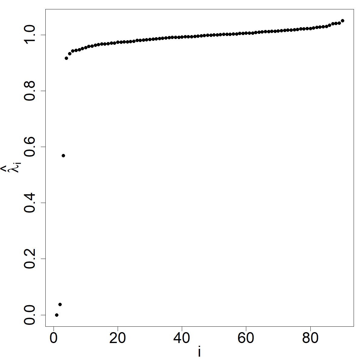
((a)) eigenvalues of $\hat{L}$

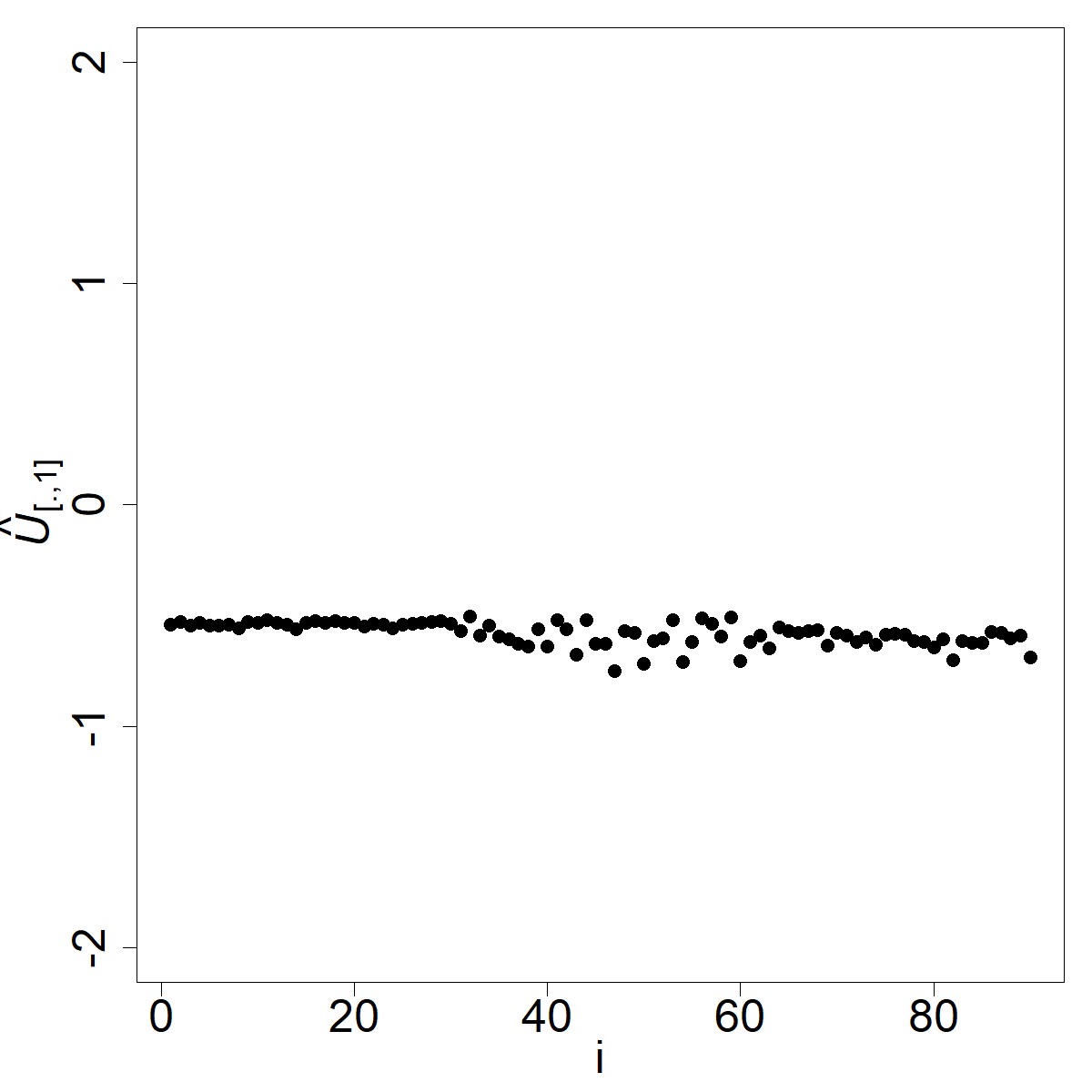
((b)) eigenvector $\hat{\mathcal{U}}_{\cdot,1}$

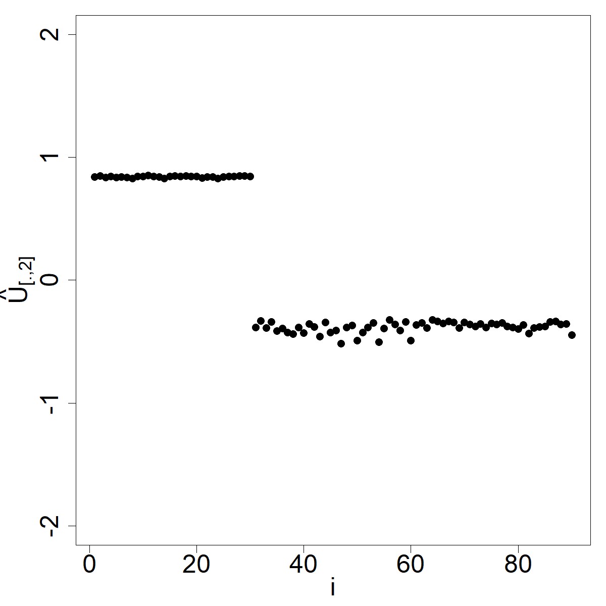
((c)) eigenvector $\hat{\mathcal{U}}_{\cdot,2}$

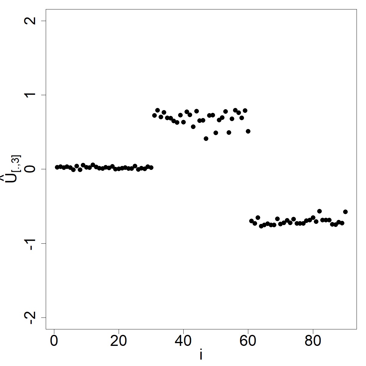
((d)) eigenvector $\hat{\mathcal{U}}_{\cdot,3}$

Figure 3.3: The spectrum of $\hat{L}$ and the three row-normalized eigenvectors belonging to the eigenvalues that belong to the three smallest eigenvalues $\hat{\lambda}_{1}\leq\hat{\lambda}_{2}\leq\hat{\lambda}_{3}$.

3.3 Clustering the embedded points using $k$-means

In this section, we analyze the final step where $k$-means is applied to the embedded points $\hat{\mathcal{U}}_{1,\cdot},\ldots$, $\hat{\mathcal{U}}_{d,\cdot}\in\ \mathbb{R}^{k}$. We show that the $k$-means algorithm, clusters, with high probability, the data correctly. More specifically, we derive a non-asymptotic bound on the number of points that are misclustered and show, under regularity conditions, that this converges to zero as $T\to\infty$.

The $k$-means objective aims to partition the $d$ embedded points $\hat{\mathcal{U}}_{1,\cdot},\ldots,\hat{\mathcal{U}}_{d,\cdot}\in\mathbb{R}^{k}$ into $k$ clusters $\{C_{1},\ldots,C_{k}\}$ in such a way that the pairwise squared deviations of points within the same cluster is minimized. The algorithm thus returns the centroids $\{c^{\star}_{1},\ldots,c^{\star}_{k}\}$ from the objective function,

$$\min_{\{c_{1},\ldots,c_{k}\}\subset\mathbb{R}^{k}}\sum_{i}\min_{j}\|\hat{\mathcal{U}}_{i,\cdot}-c_{j}\|^{2}_{2}.$$

The data points $\hat{\mathcal{U}}_{i,\cdot}$ and $\hat{\mathcal{U}}_{j,\cdot}$ are then put in the same cluster if $c^{\star}_{i}=c^{\star}_{j}$. More formally but equivalently, for $\hat{\mathcal{U}}$ defined in (3.5), the $k$ means algorihm should return a matrix $C^{\star}\in\mathbb{R}^{d\times k}$ with at most $k$ unique rows such that

$$C^{\star}=\operatorname*{arg\,min}_{C\in\mathcal{M}(d,k)}\|\hat{\mathcal{U}}-C\|^{2}_{2}.$$ (3.6)

where $\mathcal{M}(d,k)=\{M\in\mathbb{R}^{d\times k}:M\text{ has at most $k$ distinct rows}\}$.

To analyze the algorithm, we need to define what we mean with a point being correctly clustered. Let $C^{\star}$ as in (3.6), i.e., the matrix returned from applying the $k$-means algorithm to $\hat{\mathcal{U}}$. Intuitively, a point $\hat{\mathcal{U}}_{i,\cdot}$ is correctly clustered if there is no other row of the population matrix $\mathcal{U}$ defined in (3.4) that is closer to $C^{\star}_{i,\cdot}$ than the $i$-th row. Using this intuition, we can provide a meaningful definition of the set of correctly clustered point (Lemma C.2) and hence of its complement set. The next theorem gives a nonasymptotic bound on the number of misclustered points.

Theorem 3.1.

Assume the graph has $k$ components. Then the cardinality of the set of misclustered points, denoted by $|\Sigma|$, satisfies

$$|\Sigma|\leq\iota k\frac{1}{\min_{i}\|{U}_{i,\cdot}\|^{2}_{2}}\frac{\rvert\rvert\rvert{\hat{L}-L}\rvert\rvert\rvert^{2}_{\infty}}{\lambda^{2}_{k+1}}\leq\iota k{\frac{\mathcal{C_{\text{max}}}}{\min_{i}D_{i}}}\frac{\rvert\rvert\rvert{\hat{L}-L}\rvert\rvert\rvert^{2}_{\infty}}{\lambda^{2}_{k+1}}.$$ (3.7)

for some constant $\iota>0$ and where $\mathcal{C_{\text{max}}}=\max_{i}\sum_{i_{1}\in G_{i}}\sum_{i_{2}\in G_{i}}W_{i_{1},i_{2}}$. If the conditions underlying Theorem 2.1 hold, then $|\Sigma|$ converges to zero in probability as $T\to\infty$.

This upper bound implies that the probability of misclustering is affected by various properties of the (data-induced) graph. Firstly, one can see it is an increasing function of the number of clusters $k$. Secondly, it is a decreasing function of the minimum degree. In particular, the second inequality implies that for an unbalanced graph as measured by the maximal sum of all entries of any of the groups relative to the minimal degree $\min_{i}D_{i}$ the probability to miscluster has a less tight upper bound. In other words, if the graph contains isolated vertices and or many points that are highly concentrated, we can expect a higher probability to miscluster. Thirdly, it is a decreasing function of the distance between the zero eigenvalues and the first nonzero eigenvalue $\lambda_{k+1}$. Finally, it is affected by how well $\hat{L}$ estimates $L$.

Example (continued).

For our example, the embedded points are shown in the left graph of Figure 3.4. Applying k-means identifies all clusters exactly where the colors indicate the cluster the respective data points belong to.

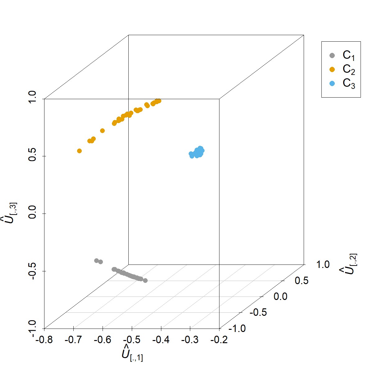
Figure 3.4: The embedded points $\hat{\mathcal{U}}_{[1,\cdot]},\ldots,\hat{\mathcal{U}}_{[90,\cdot]}$ (left) and the result of applying $k$-means to these points where the color indicate the cluster the point belongs to (right).

3.4 The choice of $k$

So far we have considered the case where the number of clusters $k$ is known. In the remaining part of this section we briefly discuss a data driven choice of $k$. This problem has received much attention within the clustering literature and a wide range of methods has been developed (see Gordon, 1999; Theodoridis and Koutroumbas, 2008, for overviews) and compared (see Milligan and Cooper, 1985; Tibshirani et al., 2001, and references therein). Most methods to pick $k$ are formulated in terms of optimizing a relative criteria. For different choices of $k$, the quality of the clustering structure is evaluated according to some measure, such as the intra-cluster dispersion, and the number of clusters chosen that optimizes this criteria.

There is however no universally optimal method because the definition of ‘optimal’ number of clusters can highly depend on the application and on the method used to cluster to data. If the data is well-separated and there are clear pronounced clusters then there are several successful methods that will correctly detect the underlying clusters. However, in noisy datasets with overlapping of clusters, different methods will detect different number of clusters. In the case of spectral clustering, an intuitive alternative would be to pick the number of clusters $k$ such that the first $\lambda_{1},\ldots,\lambda_{k}$ eigenvalues of $\hat{L}$ are small but $\lambda_{k+1}$ is ‘relatively’ large. This ‘eigengap’ heuristic can be justified through spectral properties of the population graph Laplacian and Lemma 3.1. In practice it is however also known to be very sensitive to the construction of the similarity graph and can quickly fail unless the data is well separated. Deemed therefore an unsolvable problem, it is not uncommon to apply multiple criteria and pick the criteria that works best for the particular problem at hand (see Charrad et al., 2014, for an implementation of various criteria).

A thorough development of a new method would be beyond the scope of this paper. In our empirical study in 5 we investigate the performance of available methods to choose $k$ for our particular algorithm. Additionally, we consider two variations of the eigengap heuristic each with a different interpretation of a “relatively large” eigengap.

4 Testing for equality

Besides from the application of the similarity measure as a basis for spectral clustering of functional time series, a well-defined limiting distribution allows it to be meaningful in a variety of statistical applications and in particular for the construction of hypothesis tests. The problem to detect similarities or to compare time series is of interest in a wide range of scientific fields and for classical time series a variety of methods have been proposed (see references in the introduction and examples therein). In case of functional data, the literature is less well-developed. Horvàth et al. (2013) proposed a procedure to test the hypothesis that two sets of functional data are identical and independently distributed using the sum of $L^{2}$-distances of the sequence of correlation functions. Panaretos and Tavakoli (2016) instead proposed a test between two stationary functional time series based upon the Hilbert-Schmidt norm of the difference of the sample spectral density operators, restricted to a Hilbert-Schmid space of finite dimension. Bootstrap-based methods to test for equality of mean functions or covariance operators are proposed in Paporoditis and Sapatinas (2016) and, more recently, Leucht et al. (2018) disucssed a test for the equality of spectral density operators.

To our knowledge, no procedure is available that allows to test for similarity of functional time series of which the second order structure is allowed to be time-dependent. In this section, we develop such a test using the previously defined similarity measure ${\mathcal{A}}_{i_{1},i_{2}}$ in (2.3). For the sake of brevity we restrict ourselves to the case of two functional series and consider the hypothesis

$$H_{0}:\mathcal{F}^{(i_{1})}_{u,\omega}\equiv\mathcal{F}^{(i_{2})}_{\omega}\hskip 7.22743pt\text{a.e. on }[-\pi,\pi]\times[0,1]$$ (5.1)

versus

$$H_{a}:\mathcal{F}^{(i_{1})}_{u,\omega}\neq\mathcal{F}^{(i_{2})}_{\omega}\text{on a subset of }[-\pi,\pi]\times[0,1]\text{ of positive Lebesgue measure}$$ (5.2)

The similarity measure in (2.3) lends itself quite naturally to test this hypothesis, i.e., we can equivalently formulate the hypothesis as

$$H_{0}:{\mathcal{A}}_{i_{1},i_{2}}=0\hskip 21.68121pt\text{versus}\hskip 21.68121ptH_{a}:{\mathcal{A}}_{i_{1},i_{2}}>0.$$ (5.3)

By Theorem 2.1, the statistic $\hat{\mathcal{A}}_{i_{1},i_{2}}$ defined in (2.7) is a consistent estimator of the normalized distance ${\mathcal{A}}_{i_{1},i_{2}}$. Therefore it is reasonable to reject the null hypothesis for large values of the estimator $\hat{\mathcal{A}}_{i_{1},i_{2}}$. Using the set of reqularity conditions provided in Appendix Appendix B the following result gives the asymptotic distribution of $\hat{\mathcal{A}}_{i_{1},i_{2}}$.

Theorem 4.1.

Suppose that Assumption B.1 with $m\geq 1$ and Assumption B.2 hold. Then,

$$\left\{\sqrt{T}\left(\hat{\mathcal{A}}_{i_{1},i_{2}}-\mathcal{A}_{i_{1},i_{2}}\right)\right\}_{\{i_{1},i_{2}\in[d]\}}\to\mathcal{N}(\boldsymbol{0},\boldsymbol{\Gamma})\quad\text{ as }T\to\infty,$$

where $\boldsymbol{0}\in\mathbb{R}^{d}$ and $\boldsymbol{\Gamma}$ is a positive definite element of $\,\mathbb{R}^{d\times d}$.

Under the null hypothesis, the asymptotic variance reduces to a very succinct form in case the processes are moreover independent.

Theorem 4.2.

Suppose that Assumption B.1 with $m\geq 1$ and Assumption B.2 hold and suppose $\{X_{i_{1},t,T}\}$ and $\{X_{i_{2},t,T}\}$ are independent. Then, under the null hypothesis $H_{0}:\mathcal{F}^{i_{1}}_{u,\omega}\equiv\mathcal{F}^{i_{2}}_{u,\omega}$, we have

$$\sqrt{T}\hat{\mathcal{A}}_{i_{1},i_{2}}\sim\mathcal{N}\big{(}0,\sigma^{2}_{H_{0}}\big{)},$$

where the asymptotic variance is given by

$$\sigma^{2}_{H_{0}}=4\pi\frac{\int_{-\pi}^{\pi}\int_{0}^{1}\rvert\rvert\rvert{\mathcal{F}^{i_{1}}_{u,\omega}}\rvert\rvert\rvert^{4}_{2}dud\omega}{\big{(}\int_{-\pi}^{\pi}\int_{0}^{1}\rvert\rvert\rvert{\mathcal{F}^{i_{1}}_{u,\omega}}\rvert\rvert\rvert^{2}_{2}dud\omega\big{)}^{2}}.$$ (5.4)

Let $I_{p}^{u_{j},\omega_{k}}=(I_{i_{1}}^{u_{j},\omega_{k}}+I_{i_{2}}^{u_{j},\omega_{k}})/2$ be the pooled periodogram operator evaluated at $u_{j}$ and $\omega_{k}$. The asymptotic variance under the null can be estimated by

$$\hat{\sigma}_{H_{0}}^{2}=\frac{2}{3T}\sum_{j=1}^{M}\sum_{k=1}^{\lfloor N/2\rfloor}\big{(}\langle I_{p}^{u_{j},\omega_{k}},I_{p}^{u_{j},\omega_{k-1}}\rangle_{HS}\big{)}^{2}\Big{/}\Big{(}\frac{2}{T}\sum_{j=1}^{M}\sum_{k=1}^{\lfloor N/2\rfloor}\langle I_{p}^{u_{j},\omega_{k}},I_{p}^{u_{j},\omega_{k-1}}\rangle_{HS}\Big{)}^{2}.$$ (5.5)

Lemma 4.1.

Under the conditions of Theorem 4.2, the estimator defined in (5.5) satisfies

$$\hat{\sigma}_{H_{0}}^{2}\overset{p}{\to}\sigma_{H_{0}}^{2}$$

as $T\to\infty$.

Consequently, a test for the hypotheses (5.1) and (5.2) can be based upon rejecting the null if

$$\hat{\mathcal{A}}_{i_{1},i_{2}}~{}>~{}\frac{\hat{\sigma}^{2}_{H_{0}}}{\sqrt{T}}z_{1-\alpha}~{},$$ (5.6)

where $z_{1-\alpha}$ denotes the $({1-\alpha})$-quantile of the standard normal distribution. The finite sample performance of this test is studied in a simulation study which is provided at the end of Section 5.

Remark 4.1.

We emphasize that Theorem 4.2 still holds in case the series are dependent but the expression of the asymptotic variance is slightly more involved. It can however still be estimated similar in spirit to (5.5). See Appendix Appendix B for more details.

5 Simulation study

To study the performance in finite samples, we apply the algorithm to a mixture of stationary and non-stationary models in a variety of settings. We vary the number of clusters $k$ and the number of observations per cluster $n$ as well as the included models. The algorithm is moreover considered both in the case were the number of true clusters are known and when this is unknown. In the latter case, we obtain an additional source of variability as the number of clusters needs to be estimated from the data. Finally, we consider the effect on the simulations of applying a scaling factor $\eta$ to our similarity matrix. Before we discuss how to determine $k$, we start by introducing the simulation setting and data-generating processes.

5.1 Simulation setting

We simulate functional autoregressive and functional moving average via their bais representation as follows. A $p$-th order (time varying) functional autoregressive process (tvFAR(p)), $(X_{t},t\in\mathbb{Z})$ can be defined as

$$X_{t}=\sum_{t^{\prime}=1}^{p}A_{t,t^{\prime}}(X_{t-t^{\prime}})+\epsilon_{t},$$ (4.1)

where $A_{t,1},\dots,A_{t,p}$ are time-varying autoregressive operators on $L^{2}([0,1])$ and $\{\epsilon_{t}(\tau)\}_{t\in\mathbb{Z}}$ is a sequence of mean zero innovations taking values in $L^{2}([0,1])$. To generate such processes, let $\{\psi_{l}\}_{l=1}^{\infty}$ be a Fourier basis of $L^{2}([0,1])$. By means of a basis expansion, one can show that (see e.g., Aue and van Delft, 2017) the first $L_{max}$ coefficients of (4.1) are generated using the $p$-th order vector autoregressive, VAR(p), process

$$\widetilde{X}_{t}=\sum_{t^{\prime}=1}^{p}\widetilde{A}_{t,t^{\prime}}\widetilde{X}_{t-t^{\prime}}+\widetilde{\epsilon}_{t},$$

where $\widetilde{X}_{t}:=\left(\langle X_{t},\psi_{1}\rangle,\dots,\langle X_{t},\psi_{L_{max}}\rangle\right)^{\top}$ is the vector of basis coefficients and the $(l,l^{\prime})$-th entry of $\widetilde{A}_{t,j}$ is given by $\langle A_{t,j}(\psi_{l}),\psi_{l^{\prime}}\rangle$ and $\widetilde{\epsilon}_{t}:=\left(\langle\epsilon_{t},\psi_{1}\rangle,\dots,\langle\epsilon_{t},\psi_{L_{max}}\rangle\right)^{T}$. The entries of the matrix $\widetilde{A}_{t,j}$ are generated as $N\big{(}0,\nu_{l,l^{\prime}}^{(t,j)}\big{)}$ with $\nu_{l,l^{\prime}}^{(t,j)}$ specified below. To ensure stationarity or existence of a causal solution the norms $\kappa_{t,j}$ of $A_{t,j}$ are required to satisfy certain conditions (see Bosq (2000) for stationary and van Delft and Eichler (2018) for local stationary time series, respectively). We also consider the following time varying functional moving-average process or order $1$:

$$X_{t,T}=B_{1}(\epsilon_{t})-\frac{1}{2}\left(1+b\cos\left(2\pi\frac{t}{T}\right)\right)B_{2}(\epsilon_{t-1})$$ (4.2)

where $B_{1}$ and $B_{2}$ are bounded linear operators on $L^{2}([0,1])$ and $b\in\mathbb{R}$. Similarly as above, we use a basis expansion and generate data from the model

$$\widetilde{X}_{t,T}=\widetilde{B}_{1}\widetilde{\epsilon}_{t}-\frac{1}{2}\left(1+b\cos\left(2\pi\frac{t}{T}\right)\right)\widetilde{B}_{2}\widetilde{\epsilon}_{t-1}$$

where $\widetilde{X}_{t,T}=\left(\langle X_{t,T},\psi_{1}\rangle,\dots,\langle X_{t,T},\psi_{L_{max}}\rangle\right)^{T}$ is the vector of basis coefficients, the $(l,l^{\prime})$-th entry of $\widetilde{B}_{1}$ and $\widetilde{B}_{2}$ are given by $\langle B_{1}(\psi_{l}),\psi_{l^{\prime}}\rangle$ and $\langle B_{2}(\psi_{l}),\psi_{l^{\prime}}\rangle$ respectively and $\widetilde{\epsilon}_{t}$ is as above.

we consider the following data generating processes:

• The functional white noise variables $\epsilon_{1},\dots,\epsilon_{T}$ i.i.d. with coefficient variances $\text{Var}(\langle\epsilon_{t},\psi_{l}\rangle)=\exp(-(l-1)/10)$.

• A FAR(2) variables $X_{1},\dots,X_{T}$ with operators specified by variances $\nu_{l,l^{\prime}}^{(1)}=\exp(-l-l^{\prime})$ and $\nu_{l,l^{\prime}}^{(2)}=1/(l+l^{\prime 3/2})$ with norms $\kappa_{1}=0.75$ and $\kappa_{2}=-0.4$ and the innovations $\epsilon_{1},\dots,\epsilon_{T}$ are as in (I).

• A MA(1) with $b=0$ and operators specified by variances $\nu_{l,l^{\prime}}^{(1)}=\exp(-l-l^{\prime})$.

• A tvFAR(1) with operator specified by variances $\nu_{l,l^{\prime}}^{(t,1)}=\nu_{l,l^{\prime}}^{(1)}=\exp(-l-l^{\prime})$ and norm $\kappa_{1}=0.8$, and innovations are as in (I) but with a multiplicative time-varying variance

  $$\sigma^{2}(t)=\cos\Big{(}\frac{1}{2}+\cos\big{(}\frac{2\pi t}{T}\big{)}+0.3\sin\big{(}\frac{2\pi t}{T}\big{)}\Big{)}.$$

• A tvFAR(2) with operators as in (IV), but with time-varying norm

  $$\kappa_{1,t}=1.8\cos\left(1.5-\cos\left(\frac{4\pi t}{T}\right)\right)$$

  and constant norm $\kappa_{2}=-0.81$ and innovations are as in (I).

• A FAR(2) with structural break;

  • for $t\leq 3T/8$, the operators are as in (II) with norms $\kappa_{1}=0.7$ and $\kappa_{2}=0.2$, with innovations as in (I).

  • for $t>3T/8$, the operators are as in (II) with norms $\kappa_{1}=0$ and $\kappa_{2}=-0.2$, with innovations as in (I) but with coefficient variances $\text{Var}(\langle\epsilon_{t},\psi_{l}\rangle)=2\exp((l-1)/10)$.

Our simulation consists of the following settings:

1. Setting 1: $k=3$ with models I, II and III, where the replications per cluster are taken $n=10$ and $n=30$

2. Setting 2: $k=3$ with models IV, V and VI, where the replications per cluster are taken $n=10$ and $n=30$

3. Setting 3: $k=6$ with models I-VI, where the replications per cluster are taken $n=10$ and $n=30$ and $n=50$.

Per set-up, we run 500 simulations for both $T=256$ wit $M=8$ and $T=512$ with $M=16$.

For the choice of $k$ we investigated a subset of well-known classical criteria that have been demonstrated to work well in aforementioned comparison studies on classical clustering: the Silhouette Index (Kaufman and Rousseeuw, 1990), the CH Index(Calinski and Harabasz, 1974), the Hartigan Index (Hartigan, 1975) and the KL Index (Krzanowski and Lai, 1988). We respectively refer to these in the tables as ‘sil’ ,‘ch’, ‘hartigan’ and ‘kl’. Because these cannot be applied to the spectral embedding directly, the respective criteria were constructed using the similarity graph $\hat{W}$.

Additionally, we considered two variations of the eigengap heuristic each with a different interpretation of ‘relatively large’ eigengap. Let $0=\hat{\lambda}_{1}\leq\ldots\leq\hat{\lambda}_{d}$ be the estimated eigenvalues of $\hat{L}$ in ascending order

1. ‘Relgap’: define the relative contribution of the $k$-th eigenvalue as

   $$\rho_{k}=\frac{\big{(}\hat{\lambda}_{k}-\hat{\lambda}_{k-1}\big{)}}{\hat{\lambda}_{k}}.$$

   Then the rule is to pick $k^{\star}$ as the largest $k$ for which the $k$-th contribution is still larger than a threshold value that is allowed to depend on the scaling parameter $\eta$ of the graph (see (4.3) below).

   $$k^{\star}=\max_{k}\big{\{}k\in\{1,\ldots,k_{\text{max}}\}:\rho_{k}\leq 0.01\eta\big{\}}$$

2. ‘sd1gap’: let

   $$\sigma(\hat{\lambda}_{[-1:k]})=\frac{1}{d-k}\sum_{j=k+1}^{d}\big{(}\hat{\lambda}_{j}-\frac{1}{d-k}\sum_{j=k+1}^{d}\hat{\lambda}_{j}\big{)}^{2}$$

   be the squared deviation from the mean excluding the first $k$ eigenvalues. Then the rule is to pick $k^{\star}$ as the largest $k$ for which the $k$-th gap is still larger than $\sigma(\hat{\lambda}_{[-1:k]})$, i.e.,

   $$k^{\star}=\max_{k}\big{\{}k\in\{1,\ldots,k_{\text{max}}\}:\hat{\lambda}_{k+1}-\hat{\lambda}_{k}\geq\sigma(\hat{\lambda}_{[-1:k]})\big{\}}$$

For all criteria, the maximum numbers of clusters to consider was set to $k_{\max}=15$.

5.2 Simulation results

Table 1 provides the average $k$ chosen according to the different criteria in each setting, while the corresponding percentage of misclustered points averaged over simulations are given in Table 2.

From the first row for $T=256$ and $T=512$ of Table 2, we find that our algorithm does very well if the true $k$ is known as it has a very low percentage of misclustered points across the different settings. Based upon the percentage of misclustered points, the most difficult model is clearly setting 2 with $T=256$. This finding is in accordance with the upper bound in (3.7), which is less tight for larger $k$ and lower estimation precision on $\hat{L}$.

If the true $k$ is not known we obtain higher percentages of misclustered points, where the percentages appear to be directly caused by the way $k$ was selected. As can be seen from Table 1, the CH Index does best in determining the true number of clusters, while the KL index does worst when the number of true clusters increases. Both the Silhouette Index and the Hartigan Index tend to pick $k$ more conservatively. The two rules based upon the estimated eigenvalues of the graph Laplacian –‘Relgap’ and ‘sd1gap’– appear competitive with the CH index, except in setting 2 for $n=10$. What is in particular clear is the overall improvement as both $n$ and $T$ increase. It appears that in particular the eigenvalue-based methods suffer from more variation when $n$ and $T$ are small. This is intuitive, since the choice of $k$ directly depends upon the estimation precision of the spectral properties, which can be expected to be more sensitive to estimation error for small $T$ and $n$ (see also Theorem 3.1) . From the results in table Table 2, we find the CH index to work best in combination with our algorithm. It is most stable across the different settings and has the lowest percentage of misclustered points, which appears to be a direct consequence of the fact that this index estimated the true number of clusters best and that our algorithm suffers from low error conditionally upon knowing the correct number of clusters.

Table 1: chosen k per method averaged over simulations (standard deviation in brackets)

	Setting 1		Setting 2		Setting 3
method	$n=10$	$n=30$	$n=10$	$n=30$	$n=10$	$n=30$	$n=50$
$T=256$
true $k$	3	3	3	3	6	6	6
sil	2 (0)	2 (0)	3 (0.1)	3 (0)	5.34 (0.8)	5.24 (0.5)	5.17 (0.4)
ch	3 (0.5)	2.96 (0.2)	3.05 (0.2)	3 (0)	6.37 (0.6)	6.08 (0.3)	6.03 (0.2)
kl	2.19 (1.4)	2.04 (0.7)	3.09 (1)	3.22 (1.4)	10.4 (3.1)	11.13 (3.5)	10.79 (3.6)
hart	3.04 (0.2)	3 (0)	3 (0)	3 (0)	4.86 (0.9)	4.87 (0.7)	4.87 (0.6)
Relgap	3.04 (0.2)	3 (0)	3.92 (1.1)	3.09 (0.3)	5.14 (0.4)	5.15 (0.4)	5.19 (0.4)
sd1gap	3.09 (0.3)	3.03 (0.2)	3.83 (1.2)	3.55 (1)	5.65 (0.9)	6.23 (0.7)	6.41 (0.9)
$T=512$
true $k$	3	3	3	3	6	6	6
sil	2 (0)	2 (0)	3 (0)	3 (0)	5.92 (0.4)	5.95 (0.2)	5.98 (0.1)
ch	3.13 (0.4)	3 (0)	3 (0)	3 (0)	6.52 (0.7)	6.16 (0.4)	6.08 (0.3)
kl	2.44 (1.7)	2.18 (1)	3.05 (0.7)	3.43 (2.1)	9.87 (3.3)	10.45 (3.5)	9.47 (3.5)
hart	3 (0)	3 (0)	3 (0)	3 (0)	5.28 (0.7)	5.4 (0.6)	5.43 (0.5)
Relgap	3 (0)	3 (0)	3.57 (0.8)	3.03 (0.2)	5.53 (0.6)	5.88 (0.3)	5.99 (0.1)
sd1gap	3.09 (0.4)	3.01 (0.1)	3.92 (1.2)	3.4 (0.8)	6.38 (0.9)	6.3 (0.6)	6.2 (0.5)

Table 2: percentage of misclustered points of the spectral clustering algorithm averaged over simulations (standard deviation in brackets

	Setting 1		Setting 2		Setting 3
method	$n=10$	$n=30$	$n=10$	$n=30$	$n=10$	$n=30$	$n=50$
$T=256$
true	0.11 (0.6)	0.05 (0.2)	0.01 (0.1)	0 (0)	3.22 (6.6)	0.3 (1.1)	0.13 (0.2)
sil	33.33 (0)	33.33 (0)	0.03 (0.4)	0 (0)	13.16 (10.2)	12.97 (8.2)	13.87 (6.9)
ch	4.65 (10.4)	1.41 (6.6)	0.49 (2.6)	0 (0)	5.11 (6.8)	0.82 (2.2)	0.31 (1.1)
kl	33.3 (6.4)	33.48 (2.4)	0.55 (6)	1.45 (9.4)	25.6 (14.7)	25.93 (15.6)	22.59 (14.4)
hart	0.61 (2.6)	0.05 (0.2)	0.01 (0.1)	0 (0)	19.76 (14.6)	18.93 (12.5)	19.02 (10.7)
Relgap	0.57 (2.4)	0.05 (0.2)	10.78 (11.9)	1.27 (4.2)	15.75 (5.6)	14.49 (6.3)	13.68 (6.7)
sd1gap	1.33 (4)	0.46 (2.3)	9.11 (12.5)	6.55 (10.9)	12.33 (7.5)	3.02 (5.5)	2.79 (5.2)
$T=512$
true	0 (0)	0 (0)	0 (0)	0 (0)	0.23 (1.7)	0.01 (0.1)	0 (0)
sil	33.33 (0)	33.33 (0)	0.03 (0.4)	0 (0)	2.68 (5.8)	0.77 (3.5)	0.37 (2.4)
ch	1.67 (4.6)	0 (0)	0.44 (2.1)	0 (0)	3.42 (4.4)	1.14 (2.6)	0.61 (2)
kl	27.97 (14.5)	30.63 (10.2)	1.68 (10.3)	2.59 (12.5)	20.93 (16.8)	21.37 (16.3)	15.56 (14.4)
hart	0 (0)	0 (0)	0 (0)	0 (0)	12.25 (12.1)	9.98 (9.4)	9.57 (8.7)
Relgap	0.02 (0.4)	0 (0)	6.92 (9.7)	0.39 (2.2)	8.73 (8.4)	2 (5.4)	0.17 (1.7)
sd1gap	1.13 (4.4)	0.14 (1.4)	10.16 (12.6)	4.99 (9.7)	4.15 (6)	1.92 (3.9)	1.42 (3.4)

As explained in Section 2, we apply a local scaling to avoid sensitivity on a global scaling parameter. To investigate the robustness with respect to scaling, we consider our clustering algorithm as explained in Section 3 but with an additional scaling parameter $\eta$ in the construction of the adjacency matrix. That is, we consider the simulations but with

$$\hat{W}=e^{-\eta\hat{\mathcal{A}}}\in\mathbb{R}^{d\times d}.$$ (4.3)

where $\eta=\{0.5,2.5,5,10\}$. The results in Table 2 correspond to the choice $\eta=1$ and in Table 3 we present the four alternative choices. Because of space constraints, we only report them for the specification $T=512$ and $n=30$. The results for the other cases show a very similar picture and are available upon request. It can be observed from the first row for each of the settings that the outcomes are fairly similar when $k$ is known. Variation again therefore seems mostly caused by the way $k$ is chosen, where we find the Silhouette index is sensitive as well as the KL index, but also the eigengap heuristics show some sensitivity for $\eta=10$. Overall, we may conclude that our method seems capable to detect the correct number of clusters, despite the highly complicated nature of the data. The numerical study moreover suggests that the CH index should be used to find the numbers of clusters if these are unknown.

Table 3: Percentage of misclustered points and specified $k$ for various values of $\eta$ averaged over simulations (standard deviation in brackets) for $T=512$, $n=30$

meth.	% of misclustered points				average chosen $k$
	$\eta=0.5$	$\eta=2.5$	$\eta=5$	$\eta=10$	$\eta=0.5$	$\eta=2.5$	$\eta=5$	$\eta=10$
Setting 1: $T=512,n=30$
true	0(0)	0(0)	0(0)	0(0)	3(0)	3(0)	3(0)	3(0)
sil	33.33(0)	33.33(0)	2.13(8.2)	0(0)	2(0)	2(0)	2(0)	2.94(0.2)
ch	0.03(0.6)	0(0)	0(0)	0(0)	3(0)	3(0)	3(0)	3(0)
kl	33.02(5.1)	2.8(9.3)	0(0)	0.27(4.3)	2.08(0.9)	2.18(1)	2.92(0.3)	3(0)
hart	0(0)	0(0)	0(0)	0(0)	3(0)	3(0)	3(0)	3(0)
Relgap	0(0)	0.02(0.5)	0.02(0.5)	0.03(0.5)	3(0)	3(0)	3(0)	3(0)
sd1gap	0.05(0.8)	0.88(3.5)	1.08(3.9)	0.6(2.7)	3(0.1)	3.01(0.1)	3.07(0.3)	3.09(0.3)
Setting 2: $T=512,n=30$
true	0(0)	0(0)	0(0)	0(0)	3(0)	3(0)	3(0)	3(0)
sil	0(0)	0(0)	0(0)	0(0)	3(0)	3(0)	3(0)	3(0)
ch	0(0)	0(0)	0(0)	0(0)	3(0)	3(0)	3(0)	3(0)
kl	0.35(4.6)	2.44(11.2)	1.58(9.4)	0.36(4.6)	3.05(0.7)	3.43(2.1)	3.43(2)	3.29(1.7)
hart	0(0)	0(0)	0(0)	0(0)	3(0)	3(0)	3(0)	3(0)
Relgap	0.1(1.2)	2.28(5.8)	6.66(9.3)	7.14(8.5)	3.01(0.1)	3.03(0.2)	3.18(0.5)	3.59(0.9)
sd1gap	4.75(9.5)	5.48(9.7)	4.58(8.7)	2.89(5.9)	3.38(0.8)	3.4(0.8)	3.45(0.9)	3.42(0.8)
Setting 3: $T=512,n=30$
true	0.01(0.1)	0(0)	0.04(0.9)	0.06(0.9)	6(0)	6(0)	6(0)	6(0)
sil	1.03(3.9)	0.03(0.7)	0.04(0.9)	0.06(0.9)	5.95(0.2)	5.95(0.2)	6(0)	6(0)
ch	1.65(3.2)	0.29(1.4)	0.04(0.9)	0.06(0.9)	6.23(0.5)	6.16(0.4)	6.04(0.2)	6(0)
kl	22.72(16.4)	13.94(15.5)	7.4(12.2)	4.56(10.5)	10.54(3.4)	10.45(3.5)	9.2(3.6)	7.84(3.1)
hart	11.48(8)	7.17(13.5)	0.04(0.9)	0.06(0.9)	5.31(0.5)	5.4(0.6)	5.57(0.8)	6(0)
Relgap	7.17(8.3)	0.57(2.2)	3.18(3.9)	3.93(4.4)	5.57(0.5)	5.88(0.3)	6.06(0.3)	6.57(0.8)
sd1gap	1.39(3.4)	4.5(5.1)	6.02(5.6)	4.18(5.1)	6.21(0.5)	6.3(0.6)	6.77(1)	7.2(1.3)

5.3 Testing for equality

We conclude this section with a small investigation of the proposed asymptotic $\alpha$-level test in (5.6) for the hypothesis of equality of (possibly) time-varying spectral density operators. To investigate the finite samples properties of the test, we performed a simulation study which includes the previously defined stationary models I and II and nonstationary models V and VI with parameter specification $T=512$ and $M=16$. The pairwise rejection probabilities at the $5\%$ and $10\%$ over $1000$ replications are provided in Table 4, where the diagonal elements correspond to the null hypothesis. We observe a good approximation of the nominal level with model II a bit undersized. The off-diagonal shows good power overall, with model II and model I appearing to be more difficult to distinguish than the other choices. Regardless of the second-order properties being time-varying or not, it appears therefore that the quantiles of the normal distribution are well-captured for the various models if $H_{0}$ is true, while good power is observed under $H_{A}$.

	I	II	V	VI
I	10.8	96.6	100.0	100.0
II	96.6	8.0	99.9	100.0
V	100.0	99.9	9.8	100.0
VI	100.0	100.0	100.0	10.0

	I	II	V	VI
I	5.4	93.1	100.0	100.0
II	93.1	3.2	99.7	100.0
V	100.0	99.7	3.6	100.0
VI	100.0	100.0	100.0	4.7

Table 4: Rejection probabilities of the pairwise equality test (5.6) at the 10% (left); and 5% level.

6 Data Application

We illustrate our clustering algorithm by means of an application to high resolution infrared surface temperature measurements recorded during the years 2015-2018 in the conterminous U.S., Alaska and Hawaii. The exact locations of the 126 included stations in our study are depicted in Figure 6.1.

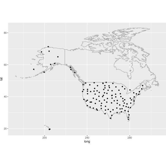
Figure 6.1: Measurement stations projected upon the map of North America acording to their longitude (long) and latitude (lat) coordinates.

.

The measurements are part of a quality controlled dataset (Diamond et al., 2013) monitored within the United States Climate Reference Network (USCRN). These are publicly available on the website of the NOAA U.S. government agency.
Understanding the characteristics of land surface temperature is of interest in various applications as it influences for example surface energy balance and various soil hydrologic processes. Our goal is to investigate whether we can identify spatial or geographical patterns in terms of variation in the surface temperature. Variation in surface temperature can be expected to be influenced by numerous factors such as wind, elevation, proximity of major water bodies or yet land cover types. For each location $i=1,\ldots,126$, we have of a sample of observations $\{X_{i,t}(\tau_{1}),\ldots,X_{i,t}(\tau_{\text{max}})\}_{t=1,\ldots,1288}$, where $X_{i,t}$ represents the sampled temperature curve on day $t$ for location $i$. The first measurement day $t=1$ corresponds to February 28 2015 and the last measurement day $t=T=1288$ corresponds to September 7 2018. The recordings were made at a 5 minute time-interval leading to a maximum of $288$ observations per day. We remark that the measurement stations included have at most 10% of missing observations per day over the measurement period. The gridded observations were transformed into functional objects using 21 Fourier basis functions, rescaled to the unit interval, i.e., $\tau_{1}$ corresponds to local time 0.00am and $\tau_{288}=\tau_{max}$ to local time 23.55pm. A few sets of realized curves are depicted in Figure 6.3.

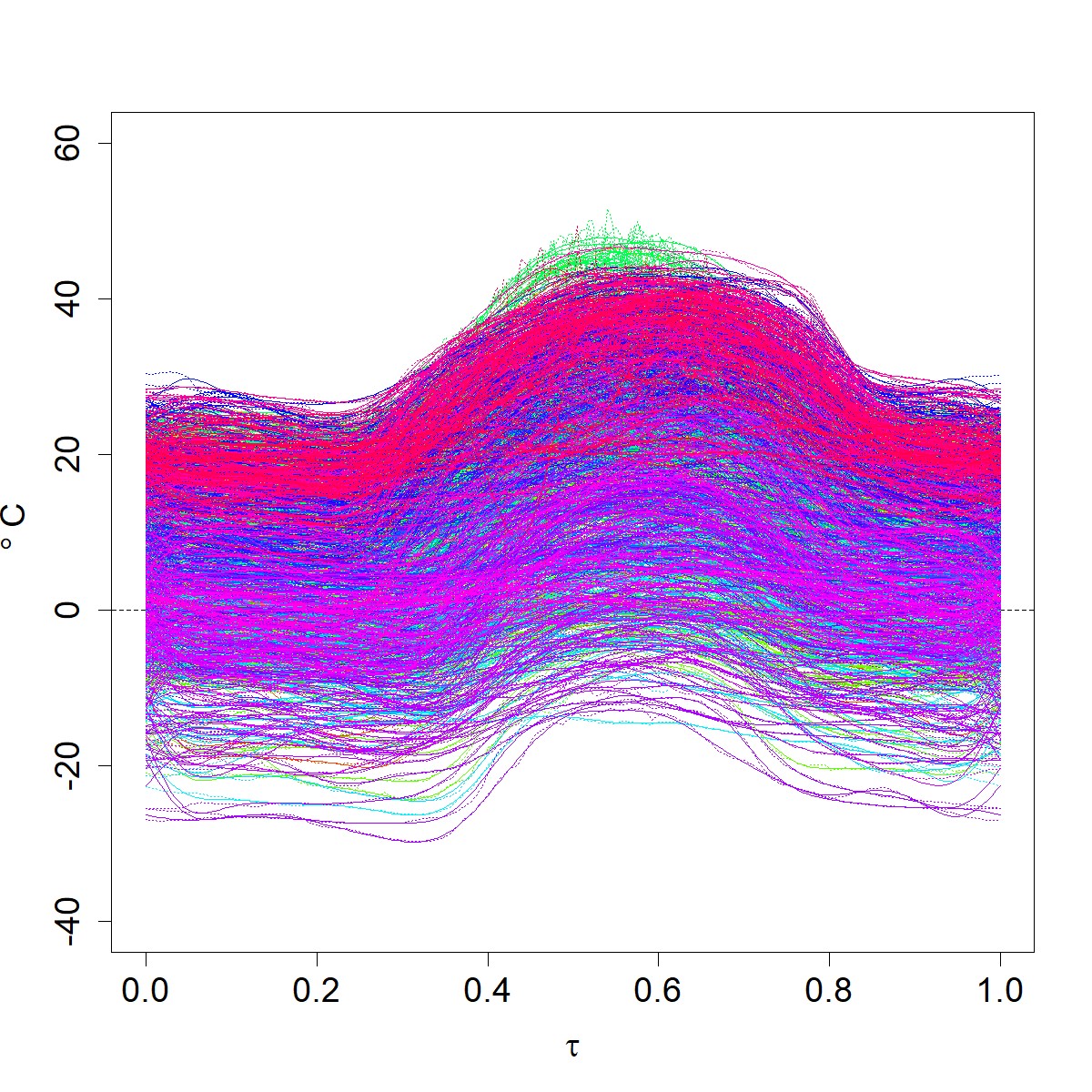
((a)) Lincoln, Nebraska

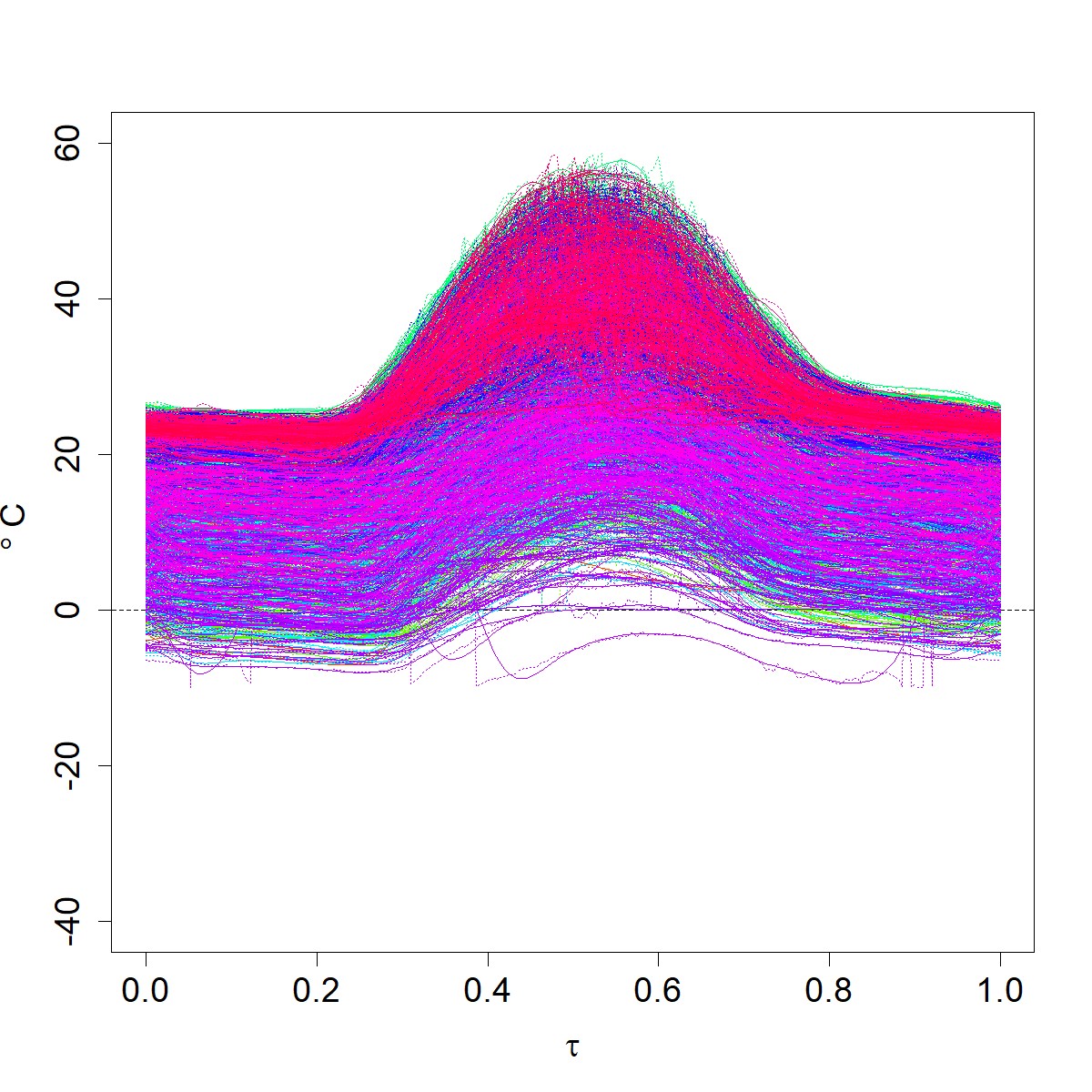
((b)) Selma, Alabama

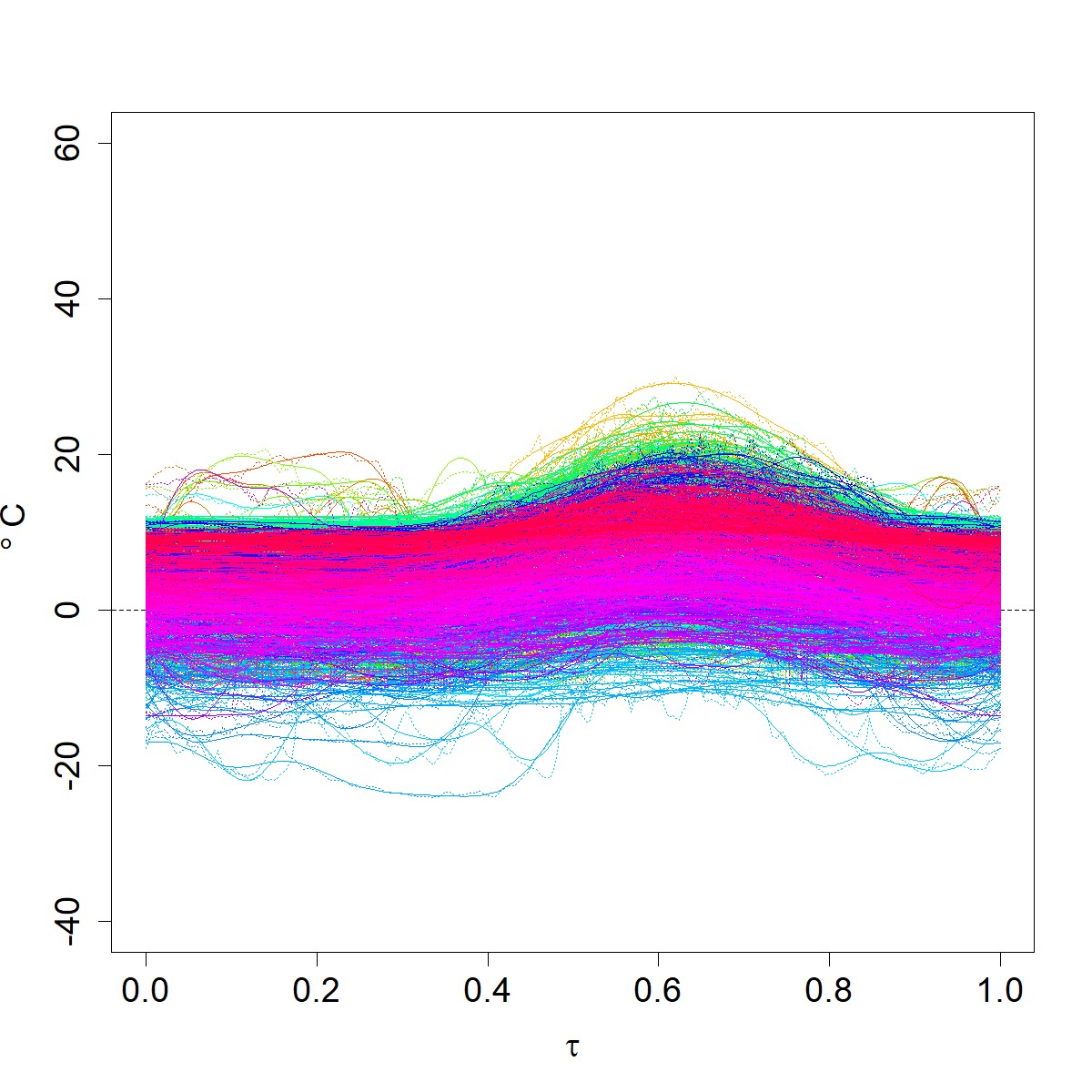
((c)) St. Paul, Alaska

Figure 6.3: Daily surface temperature curves (solid) fitted to the observations (dotted) for the period 28-Feb. 2015-07 Sept. 2018.

It can be observed there is more between-curves variation for Lincoln, Nebraska while there is more within-curve variation for Selma, Alabama. For St. Paul, the more visible variety in colors indicate a stronger variation over longer periods of time. To cluster the locations, we factorize the 1288 daily curves into $M=14$ complete seasons, each of length $N=92$. We applied our algorithm described in Section 3. For the choice of $k$, we looked at the various criteria discussed in the previous section. These indicated 2 to 4 clusters, with the majority picking 3 clusters. To choose the number of clusters, we used the index that performed best in the simulation study, which was the CH index and which indicates 3 clusters. The results of clustering the locations in 3 clusters by means of our algorithm are given in Figure 6.3. The figure seems to indicate the seasonal variation for two clusters is related to two prevailing wind patterns; those in red to the westerlies wind, while those in green to northeasterly trade wind. We moreover observe a separate cluster consisting of mainly locations on the coast in a bay area, island or on a peninsula. In particular, these locations correspond to areas known to be more affected by different atmospheric pressures which are responsible for forming cyclones and that can vary with the El Niño-Southern Oscillations cycle. It is worth remarking that a similar pattern was observed when different time periods were considered.

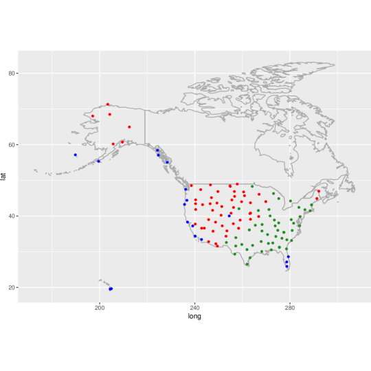
Figure 6.3: Measurement stations clustered according to variation in surface temperature

.

Acknowledgements This work has been supported in part by the Collaborative Research Center “Statistical modeling of nonlinear dynamic processes” (SFB 823, Teilprojekt A1, A7, C1) of the German Research Foundation (DFG).

Appendix A Background material and auxiliary results

Let $\mathcal{H}_{i}$ for each $i=1,\ldots,n$ be a Hilbert space with inner product $\langle\cdot,\cdot\rangle$. The tensor of these is denoted by

$$\mathcal{H}:=\mathcal{H}_{1}\otimes\ldots\otimes\mathcal{H}_{n}=\bigotimes_{i=1}^{n}\mathcal{H}_{i}$$

If $\mathcal{H}_{i}=\mathcal{H}\,\forall i$, then this is the n-th fold tensor product of $\mathcal{H}$. For $A_{i}\in H_{i},1\leq i\leq n$ the object $\bigotimes_{i=1}^{n}A_{i}$ is a multi-antilinear functional that generates a linear manifold, the usual algebraic tensor product of vector spaces $\mathcal{H}_{i}$, to which the scalar product

$$\langle\bigotimes_{i=1}^{n}A_{i},\bigotimes_{i=1}^{n}B_{i}\rangle=\prod_{i=1}^{n}\langle A_{i},B_{i}\rangle$$

can be extended to a pre-Hilbert space. The completion of the above algebraic tensor product is $\bigotimes_{i=1}^{n}\mathcal{H}_{i}$.
For $A,B,C\in\mathcal{L}(\mathcal{H})$ we define the following bounded linear mappings. The kronecker product is defined as $(A\widetilde{\bigotimes}B)C=ACB^{\dagger}$, while the transpose Kronecker product is given by $(A\widetilde{\bigotimes}_{\top}B)C=(A\widetilde{\bigotimes}\overline{B})\overline{C}^{\dagger}$. For $A,B,C\in S_{2}(\mathcal{H})$, we shall denote, in analogy to elements $a,b\in\mathcal{H}$, the Hilbert tensor product as $A\bigotimes B$. We list the following useful properties:

Properties A.1.

Let $\mathcal{H}_{i}=L^{2}_{\mathbb{C}}([0,1]^{k})$ for $i=1,\ldots,n$. Then for $a_{i},b_{i}\in\mathcal{H}_{i}$ and $A_{i},B_{i}\in S_{2}(\mathcal{H}_{i})$, we have

1. $\langle A,B\rangle_{HS}=\operatorname{Tr}({A}{B}^{\dagger})$

2. $\langle\bigotimes_{i=1}^{n}A_{i},\bigotimes_{i=1}^{n}B_{i}\rangle_{{HS}}=\prod_{i=1}^{n}\langle A_{i},B_{i}\rangle_{HS}$

3. $\langle a_{1}\otimes a_{2},b_{1}\otimes b_{2}\rangle_{HS}=\langle a_{1}\otimes\overline{a}_{2},b_{1}\otimes\overline{b_{2}}\rangle_{\mathcal{H}_{i}\otimes\mathcal{H}_{i}}=\langle a_{1},b_{1}\rangle\overline{\langle a_{2},b_{2}\rangle}$

4. If $A_{i}\in S_{1}(H)$, then $\prod_{i=1}^{n}\operatorname{Tr}(A_{i})=\operatorname{Tr}(\widetilde{\bigotimes}_{i=1}^{n}A_{i})$

5. $\big{(}(a_{1}\otimes\overline{a}_{2})\bigotimes(a_{3}\otimes\overline{a}_{4})\big{)}=\big{(}(a_{1}\otimes{a}_{3})\widetilde{\bigotimes}(\overline{a}_{2}\otimes\overline{a}_{4})\big{)}=\big{(}(a_{1}\otimes{a}_{4})\widetilde{\bigotimes}_{\top}{a}_{2}\otimes{a}_{3})\big{)}$

Let $X$ be a random element on a probability space $(\Omega,\mathcal{A},\mathbb{P})$ that takes values in a separable Hilbert space $H$. More precisely, we endow $H$ with the topology induced by the norm on $H$ and assume that $X:\Omega\to H$ is Borel-measurable. The $k$-th order cumulant tensor is defined by (van Delft and Eichler, 2018)

$$\text{Cum}\big{(}X_{1},\ldots,X_{k}\big{)}=\sum_{l_{1},\ldots l_{k}\in\mathbb{N}}\text{Cum}\big{(}\langle X_{1},\psi_{l_{1}}\rangle,\ldots,\langle X_{k},\psi_{l_{k}}\rangle\big{)}(\psi_{l_{1}}\otimes\cdots\otimes\psi_{l_{k}}),$$ (6.2)

where $\{\psi_{l}\}_{l\in\mathbb{N}}$ is an orthonormal basis of $H$ and the cumulants on the right hand side are as usual given by

$$\text{Cum}\big{(}\langle X_{1},\psi_{l_{1}}\rangle,\ldots,\langle X_{k},\psi_{l_{k}}\rangle\big{)}=\sum_{\nu=(\nu_{1},\ldots,\nu_{p})}(-1)^{p-1}\,(p-1)!\,\prod_{r=1}^{p}\mathbb{E}\Big{[}\prod_{t\in\nu_{r}}\langle X_{t},\psi_{l_{t}}\rangle\Big{]},$$

where the summation extends over all unordered partitions $\nu$ of $\{1,\ldots,k\}$. The product theorem for cumulants (Brillinger, 1981, Theorem 2.3.2) can then be generalised (see e.g. van Delft and Eichler, 2018) to simple tensors of random elements of $H$, i.e., $X_{t}=\otimes_{j=1}^{J_{t}}X_{tj}$ with $j=1,\ldots,J_{t}$ and $t=1,\ldots,k$. The joint cumulant tensor is then be given by

$$\text{Cum}(X_{1},\ldots,X_{k})=\sum_{\nu=(\nu_{1},\ldots,\nu_{p})}S_{\nu}\Big{(}\otimes_{n=1}^{p}\text{Cum}\big{(}X_{tj}|(t,j)\in\nu_{n}\big{)}\Big{)},$$ (6.3)

where $S_{\nu}$ is the permutation that maps the components of the tensor back into the original order, that is, $S_{\nu}(\otimes_{r=1}^{p}\otimes_{(t,j)\in\nu_{r}}X_{tj})=X_{11}\otimes\cdots\otimes X_{kJ_{t}}$.

Appendix B Distributional properties of the similarity measure

In order to derive the distributional properties of $\hat{\mathcal{A}}_{i_{1},i_{2}}$ defined in (2.7), we require the following assumptions on the functional processes $\{\,X_{i,t,T}\colon t\in\mathbb{Z}\}_{T\in\mathbb{N}},i=1,\ldots,d$

Assumption B.1.

Assume $\{\,X_{i,t,T}\colon t\in\mathbb{Z}\}_{T\in\mathbb{N}}$ are $d$ locally stationary zero-mean stochastic processes taking values in $\mathcal{H}_{\mathbb{R}}$ and let $\kappa_{{m};t_{1},\ldots,t_{{m}-1}}:L^{2}([0,1]^{\lfloor m/2\rfloor})\to L^{2}([0,1]^{\lfloor\frac{m+1}{2}\rfloor})$ be a positive operator independent of $T$ such that, for all $j=1,\ldots,m-1$ and some $\ell\in\mathbb{N}$,

$$\sum_{t_{1},\ldots,t_{k-1}\in\mathbb{Z}}(1+|t_{j}|^{\ell})\rvert\rvert\rvert{\kappa_{{m};t_{1},\ldots,t_{{m}-1}}}\rvert\rvert\rvert_{1}<\infty.$$ (6.4)

Let us denote

$$Y^{(T)}_{i,t}=X_{i,t,T}-X_{i,t}^{(t/T)}\qquad\text{and}\qquad Y_{i,t}^{(u,v)}=\frac{X^{(u)}_{i,t}-X^{(v)}_{i,t}}{(u-v)}$$ (6.5)

for $T\geq 1$, $1\leq t\leq T$ and $u,v\in[0,1]$ such that $u\neq v$. Suppose furthermore that $m$-th order joint cumulants satisfy

1. $\|\text{Cum}(X_{i_{1},t_{1},T},\ldots,X_{i_{m-1},t_{m-1},T},Y^{(T)}_{i_{m},t_{m}})\|_{2}\leq\frac{1}{T}\rvert\rvert\rvert{\kappa_{m;t_{1}-t_{m},\ldots,t_{m-1}-t_{m}}}\rvert\rvert\rvert_{1}$,

2. $\|\text{Cum}(X_{i_{1},t_{1}}^{(u_{1})},\ldots,X_{i_{m-1},t_{m-1}}^{(u_{m-1})},Y_{i_{m},t_{m}}^{(u_{m},v)})\|_{2}\leq\rvert\rvert\rvert{\kappa_{m;t_{1}-t_{m},\ldots,t_{m-1}-t_{m}}}\rvert\rvert\rvert_{1}$,

3. $\sup_{u}\|\text{Cum}(X_{i_{1},t_{1}}^{(u)},\ldots,X_{i_{m-1},t_{m-1}}^{(u)},X_{i_{m},t_{m}}^{(u)})\|_{2}\leq\rvert\rvert\rvert{\kappa_{m;t_{1}-t_{m},\ldots,t_{m-1}-t_{m}}}\rvert\rvert\rvert_{1}$,

4. $\sup_{u}\|\frac{\partial^{\ell}}{\partial u^{\ell}}\text{Cum}(X_{i_{1},t_{1}}^{(u)},\ldots,X_{i_{m-1},t_{m-1}}^{(u)},X_{i_{m},t_{m}}^{(u)})\|_{2}\leq\rvert\rvert\rvert{\kappa_{m;t_{1}-t_{m},\ldots,t_{m-1}-t_{m}}}\rvert\rvert\rvert_{1}$,

We remark that if the process is in fact stationary, the dependence on localized time $u$ drops. As explained in Section 2, the estimator requires splitting the sample $T\in\mathbb{N}$ as $T=N(T)M(T)$, where $N(T)$ defines the resolution in frequency of the local fDFT and $M(T)$ controls the number of nonoverlapping local fDFT’s in (2.6). Since they correspond to the number of terms used in a Riemann sum approximating the integrals with respect to $du$ and $d\omega$ they have to be sufficiently large. We assume

Assumption B.2.

$M\to\infty$, $N\to\infty$ as $T\to\infty$, such that

$$N/M\to\infty\quad\text{and}\quad N/M^{3}\to 0$$

The number of elements in the blocks grows therefore must grow faster than the number of blocks, but slower than the cube number of blocks. The choice of the number of blocks is carefully discussed in van Delft et al. (2018), who used the integrated periodogram operators as a basis for a stationarity test.

In order to derive the results in Section 4, we require four auxiliary results, which can be proved using similar arguments as given in van Delft et al. (2018) and the proofs are therefore omitted. The first one expresses the cumulants of Hilbert-Schmidt inner products of local periodogram tensors, into the trace of cumulants of simple tensors of the local functional DFT’s.

Theorem B.1.

Let $\mathbb{E}\prod_{i_{l}\in\{1,\ldots,d\}}^{2n}\rvert\rvert\rvert{I_{i_{l}}^{u,\omega}}\rvert\rvert\rvert_{2}<\infty$ for some $n\in\mathbb{N}$ and uniformly in $u$ and $\omega$. Then for any $i_{1},\ldots,i_{2n}\in\{1,\ldots,d\}$.

Cum $$\Big{(}\langle I_{i_{1}}^{u_{j_{1}},\omega_{k_{1}}},I_{i_{2}}^{u_{j_{2}},\omega_{{k_{2}}}}\rangle_{HS},\ldots,\langle I_{i_{2n-1}}^{u_{j_{2n-1}},\omega_{k_{2n-1}}},I_{i_{2n}}^{u_{j_{2n}},\omega_{{k_{2n}}}}\rangle_{HS}\Big{)}$$

$$=\operatorname{Tr}\Big{(}\sum_{\boldsymbol{P}=P_{1}\cup\ldots\cup P_{G}}S_{\boldsymbol{P}}\Big{(}\otimes_{g=1}^{G}\operatorname{cum}\big{(}D_{i_{p}}^{u_{j_{p}},\omega_{k_{p}}}\ |p\in P_{g}\Big{)}\Big{)}.$$

where the summation is over all indecomposable partitions $\boldsymbol{P}=P_{1}\cup\ldots\cup P_{G}$ of the array

$$\begin{matrix}(1,1)&(1,2)&(1,3)&(1,4)\\ (2,1)&(2,2)&(2,3)&(2,4)\\ \vdots&&&\vdots\\ \vdots&&&\vdots\\ (n,1)&(n,2)&(n,3)&(n,4)\\ \end{matrix}$$

where $p=(l,m)$ and $i_{p}=i_{2l-\delta\{m\in\{1,2\}\}}$, $k_{p}=(-1)^{m}k_{2l-\delta{\{m\in\{1,2\}\}}}$ and $j_{p}=j_{2l-\delta{\{m\in\{1,2\}\}}}$ for $l\in\{1,\ldots,n\}$ and $m\in\{1,2,3,4\}$ and where $\delta_{\{A\}}$ equals 1 if event $A$ occurs and $0$ otherwise.

We additionally require auxiliary results on the properties of the local fDFTs.

Lemma B.1.

Suppose Assumption B.1 is satisfied $k$ moments and $\sum_{j=1}^{k}\omega_{j}\equiv 0\mod 2\pi$ then

$$\Big{\rvert}\Big{\rvert}\Big{\rvert}{\text{Cum}\left(D_{i}^{u_{j},\omega_{1}},\dots,D_{i}^{u_{j},\omega_{k}}\right)-\frac{(2\pi)^{1-k/2}}{N^{k/2-1}}\mathcal{F}_{u_{i},\omega_{1},\dots,\omega_{k-1}}}\Big{\rvert}\Big{\rvert}\Big{\rvert}_{1}=O\left(N^{-k/2}\times\frac{N}{M^{2}}\right).$$

additionally, for $|i_{1}|=|i_{2}|=k/2$, we have

$$\Big{\rvert}\Big{\rvert}\Big{\rvert}{\text{Cum}\left(D_{i}^{u_{j},\omega_{1}},\dots,D_{i}^{u_{j},\omega_{k}}\right)-\frac{(2\pi)^{1-k/2}}{N^{k/2-1}}\mathcal{F}^{i_{1},i_{2}}_{u_{i},\omega_{1},\dots,\omega_{k-1}}}\Big{\rvert}\Big{\rvert}\Big{\rvert}_{1}=O\left(N^{-k/2}\times\frac{N}{M^{2}}\right).$$

where $\mathcal{F}^{i_{1},i_{2}}_{u_{i},\omega_{1},\dots,\omega_{k-1}}$ denotes the cross spectral density operator of series $i_{1}$ and $i_{2}$ of order $k$ at time $u_{i}$.

When evaluated off the manifold, i.e., $\sum_{j=1}^{k}\omega_{j}\neq 0\mod 2\pi$, the above cumulant is of lower order (see Corollary B.1). A direct consequence of the proof of Lemma B.1 is the following corollary

Corollary B.1.

For $i_{1},\ldots,i_{k}\in\{1,\ldots,d\}$ We have for any $p\geq 1$

$$\Big{\rvert}\Big{\rvert}\Big{\rvert}{\text{Cum}\left(D_{i_{1}}^{u_{1},\omega_{1}},\dots,D_{i_{k}}^{u_{k},\omega_{k}}\right)}\Big{\rvert}\Big{\rvert}\Big{\rvert}_{p}=O\left(N^{1-k/2}\right)$$ (6.7)

uniformly in $\omega_{1},\ldots,\omega_{k}$ and $u_{1},\ldots,u_{k}$. Moreover, if $~{}\sum_{j=1}^{k}\omega_{j}~{}\neq 0\mod 2\pi$ then

$$\Big{\rvert}\Big{\rvert}\Big{\rvert}{\text{Cum}\left(D_{i_{1}}^{u_{1},\omega_{1}},\dots,D_{i_{k}}^{u_{k},\omega_{k}}\right)}\Big{\rvert}\Big{\rvert}\Big{\rvert}_{p}=O\left(N^{-k/2}\right).$$ (6.8)

Additionally, when the local fDFT’s are evaluated on different midpoints then we have the following lemma.

Lemma B.2.

If Assumption B.1 is satisfied and $|{j_{1}}-{j_{2}}|>1$ for some midpoints $u_{j_{1}}$ and $u_{j_{2}}$ then

$$\Big{\rvert}\Big{\rvert}\Big{\rvert}{\text{Cum}\left(D_{i_{1}}^{u_{1},\omega_{1}},\dots,D_{i_{k}}^{u_{k},\omega_{k}}\right)}\Big{\rvert}\Big{\rvert}\Big{\rvert}_{1}=O\left(N^{-k/2}M^{-1}\right)$$

uniformly in $\omega_{1},\ldots,\omega_{k}$.

In the following, for random variables $Y_{0},Y_{1},Y_{2},Y_{3}$ let $\operatorname{cum}_{m_{0},m_{1},m_{2},m_{3}}(Y_{0},Y_{1},Y_{2},Y_{3})$ denote the joint cumulant

$$\operatorname{cum}(\underbrace{Y_{0},\ldots,Y_{0}}_{m_{0}\ \text{times}},\underbrace{Y_{1},\ldots,Y_{1}}_{m_{1}\ \text{times}},\underbrace{Y_{2},\ldots,Y_{2}}_{m_{2}\ \text{times}},\underbrace{Y_{3},\ldots,Y_{3}}_{m_{3}\ \text{times}}),$$

where $0\leq m_{i}\leq m,i=0,1,2,3$ s.t. $\sum_{i=0}^{3}m_{i}=m$. Using the previous statements, we can derive the order of the higher order joint cumulants of elements defined in $\eqref{Fij}$.

Theorem B.2.

If Assumption B.1 is satisfied then for finite $m$

$$T^{m/2}\operatorname{cum}_{m_{0},m_{1},m_{2},m_{3}}(\hat{F}_{i_{1},i_{2}},\hat{F}_{i_{3},i_{4}},\hat{F}_{i_{5},i_{6}},\hat{F}_{i_{7},i_{8}})$$

$$\frac{1}{T^{m/2}}\sum_{k_{1},\ldots,k_{m}=1}^{\lfloor N/2\rfloor}\sum_{\begin{subarray}{c}j_{1},\ldots,j_{m}=1\end{subarray}}^{M}\operatorname{Tr}\Big{(}\sum_{\boldsymbol{P}=P_{1}\cup\ldots\cup P_{G}}S_{\boldsymbol{P}}\Big{(}\otimes_{g=1}^{G}\operatorname{cum}\big{(}D_{i_{p}}^{u_{j_{p}},\omega_{k_{p}}}\ |p\in P_{g}\Big{)}\Big{)}=O(T^{1-m/2}).$$

uniformly in $0\leq m_{i}\leq m$ s.t. $\sum_{i=0}^{3}m_{i}=m$.

Proof of Theorem B.2.

For a fixed partition $P=\{P_{1},\ldots,P_{G}\}$, let the cardinality of set $P_{g}$ be denoted by $|P_{g}|=\mathscr{C}_{g}$. By (6.7) of Corollary B.1 and Lemma B.2 an upperbound of (B.1) is given by

$$O\Big{(}T^{-m/2}\sum_{k_{1},\ldots,k_{m}=1}^{\lfloor N/2\rfloor}\sum_{\begin{subarray}{c}j_{1},\ldots,j_{m}=1\end{subarray}}^{M}\prod_{g=1}^{G}\frac{1}{N^{\mathscr{C}_{g}/2-1}}M^{-\delta_{\{\exists p_{1},p_{2}\in P_{g}:|j_{p_{1}}-j_{p_{2}}|>1\}}}\Big{)}$$ (6.9)

Similar to Lemma 4.3 of van Delft et al. (2018), we can show inductively that the indecomposability of the array (B.1) and the behavior of the joint cumulants of the local fDFT’s at different midpoints imply this is at most of order

$$O(N^{m/2}M^{-m/2}E^{m}MN^{-2m+G})=O(T^{1-m/2}N^{G-m-1}).$$

Thus, partitions of size $G\leq m+1$ will vanish as $T\to\infty$. For $G\geq m+2$, indecomposability of the array requires to stay on the frequency manifold (see equation (6.8) of Corollary B.1) and therefore imposes additional restrictions in frequency direction. It can be shown (van Delft et al., 2018, Proposition 4.1) that for a partition of size $G=m+r_{1}+1$ with $r_{1}\geq 1$ of the array (B.1) only partitions with at least $r_{1}$ restrictions in frequency direction are indecomposable if $m>2$, while if $m=2$ there must be at least 1 restriction in frequency direction. Consequently, the joint cumulant is at most of order $O(T^{1-n/2}N^{m+r_{1}+1-m-1}N^{-{r_{1}}})=O(T^{1-n/2})$. ∎

Proof of Theorem 2.1.

Using Theorem B.1 with $n=1$ implies

$$\mathbb{E}{F}_{i_{1},i_{2}} =\frac{1}{T}\sum_{k=1}^{\lfloor N/2\rfloor}\sum_{j=1}^{M}\operatorname{Tr}\Big{(}\mathbb{E}\big{[}D_{i_{1}}^{{u_{j_{{1}}}},{\omega_{k_{1}}}}\otimes D_{i_{1}}^{{u_{j_{{1}}}},{-\omega_{k_{1}}}}\otimes D_{i_{2}}^{{u_{j_{{1}}}},{-\omega_{k_{1}-1}}}\otimes D_{i_{2}}^{{u_{j_{{1}}}},{\omega_{k_{1}-1}}}\big{]}\Big{)}.$$

Rewriting this expectation in cumulant tensors, we get

$$\mathbb{E}{F}_{i_{1},i_{2}} =\frac{1}{T}\sum_{k=1}^{\lfloor N/2\rfloor}\sum_{j=1}^{M}\operatorname{Tr}\Big{(}S_{1234}\text{Cum}\big{(}(D_{i_{1}}^{{u_{j_{{1}}}},{\omega_{k_{1}}}},D_{i_{1}}^{{u_{j_{{1}}}},{-\omega_{k_{1}}}},D_{i_{2}}^{{u_{j_{{1}}}},{-\omega_{k_{1}-1}}},D_{i_{2}}^{{u_{j_{{1}}}},{\omega_{k_{1}-1}}})\big{)}$$

$$+\frac{1}{T}\sum_{k=1}^{\lfloor N/2\rfloor}\sum_{j=1}^{M}\operatorname{Tr}\Bigg{(}S_{1234}\Big{(}\text{Cum}(D_{i_{1}}^{{u_{j_{{1}}}},{\omega_{k_{1}}}},D_{i_{1}}^{{u_{j_{{1}}}},{-\omega_{k_{1}}}})\otimes\text{Cum}(D_{i_{2}}^{{u_{j_{{1}}}},{-\omega_{k_{1}-1}}},D_{i_{2}}^{{u_{j_{{1}}}},{\omega_{k_{1}-1}}})\Big{)}\Bigg{)}$$

$$+\frac{1}{T}\sum_{k=1}^{\lfloor N/2\rfloor}\sum_{j=1}^{M}\operatorname{Tr}\Bigg{(}S_{1324}\Big{(}\text{Cum}(D_{i_{1}}^{{u_{j_{{1}}}},{\omega_{k_{1}}}},D_{i_{2}}^{{u_{j_{{1}}}},{-\omega_{k_{1}-1}}})\otimes\text{Cum}(D_{i_{1}}^{{u_{j_{{1}}}},{-\omega_{k_{1}}}},D_{i_{2}}^{{u_{j_{{1}}}},{\omega_{k_{1}-1}}})\Big{)}\Bigg{)}$$

$$+\frac{1}{T}\sum_{k=1}^{\lfloor N/2\rfloor}\sum_{j=1}^{M}\operatorname{Tr}\Bigg{(}S_{1423}\Big{(}\text{Cum}(D_{i_{1}}^{{u_{j_{{1}}}},{\omega_{k_{1}}}},D_{i_{2}}^{{u_{j_{{1}}}},{\omega_{k_{1}-1}}})\otimes\text{Cum}(D_{i_{1}}^{{u_{j_{{1}}}},{-\omega_{k_{1}}}},D_{i_{2}}^{{u_{j_{{1}}}},{-\omega_{k_{1}-1}}})\Big{)}\Bigg{)}$$

By Corollary B.1 andLemma B.1 we thus find

$$\mathbb{E}{F}_{i_{1},i_{2}} =\frac{1}{T}\sum_{k=1}^{\lfloor N/2\rfloor}\sum_{j=1}^{M}\langle\mathcal{F}_{u_{j},\omega_{k}}^{i_{1}},\mathcal{F}_{u_{j},\omega_{k-1}}^{i_{2}}\rangle_{HS}+O(\frac{1}{M^{2}})+O(\frac{1}{N}).$$

Hence,

$$\lim_{N,M\to\infty}\operatorname{\mathbb{E}}F_{i_{1},i_{2}}=\frac{1}{2\pi}\int_{0}^{\pi}\int_{0}^{1}\langle\mathcal{F}_{u,\omega}^{i_{1}},\mathcal{F}_{u,\omega}^{i_{2}}\rangle_{HS}\mathrm{d}u\mathrm{d}\omega=\frac{1}{4\pi}\int_{-\pi}^{\pi}\int_{0}^{1}\langle\mathcal{F}_{u,\omega}^{i_{1}},\mathcal{F}_{u,\omega}^{i_{2}}\rangle_{HS}\mathrm{d}u\mathrm{d}\omega.$$

Secondly, we have for any $i_{1},i_{2},i_{3},i_{4}\in\{1,\ldots,d\}$

$$T\text{Cov}({F}_{i_{1},i_{2}},{F}_{i_{3},i_{4}})=T\text{Cum}\big{(}{{F}_{i_{1},i_{2}},\overline{{F}_{i_{3},i_{4}}}}\big{)}$$

Hence, if Assumption B.1 is satisfied with $m=8$, Theorem B.2 implies this term is of order $O(1)$. summarizing, we find ${F}_{i_{1},i_{1}},{F}_{i_{2},i_{2}},{F}_{i_{1},i_{2}}$ and ${F}_{i_{2},i_{1}}$ are asymptotically unbiased and jointly convergence in probability. The continuous mapping theorem establishes then that $\hat{\mathcal{A}}_{i_{1},i_{2}}$ is a $\sqrt{T}$-consistent estimator of ${\mathcal{A}}_{i_{1},i_{2}}$ for any $i_{1},i_{2},\in\{1\ldots,d\}$. ∎

Proof of Theorem 4.1.

If Assumption B.1 holds for all moments, then Theorem B.2, yields that for $m>2$

$$T^{m/2}\operatorname{cum}_{m_{0},m_{1},m_{2},m_{3}}(F_{i_{1},i_{2}},F_{i_{3},i_{4}},F_{i_{5},i_{6}},F_{i_{7},i_{8}})\to 0\quad\text{as }T\to\infty,$$

from which asymptotic joint normality of $F_{i_{1},i_{2}},F_{i_{3},i_{4}},F_{i_{5},i_{6}},F_{i_{7},i_{8}}$ follows, i.e., we have

$$\sqrt{T}\begin{pmatrix}4\pi F_{i_{1},i_{1}}-\mathbb{E}(F_{i_{1},i_{1}})\\ 4\pi F_{i_{2},i_{2}}-\mathbb{E}(F_{i_{2},i_{2}})\\ 4\pi F_{i_{1},i_{2}}-\mathbb{E}(F_{i_{1},i_{2}})\\ 4\pi F_{i_{2},i_{1}}-\mathbb{E}(F_{i_{1},i_{1}})\end{pmatrix}\longrightarrow\mathcal{N}(\mathbf{0},\boldsymbol{\Sigma}),$$

where

$$\boldsymbol{\Sigma}=\left(\begin{array}[]{cccc}\text{Var}({F}_{i_{1},i_{1}})&\text{Cov}({F}_{i_{1},i_{1}},{F}_{i_{2},i_{2}})&\text{Cov}({F}_{i_{1},i_{1}},{F}_{i_{1},i_{2}})&\text{Cov}({F}_{i_{1},i_{1}},{F}_{i_{2},i_{1}})\\ \text{Cov}({F}_{i_{1},i_{1}},{F}_{i_{2},i_{2}})&\text{Var}({F}_{i_{2},i_{2}})&\text{Cov}({F}_{i_{2},i_{2}},{F}_{i_{1},i_{2}})&\text{Cov}({F}_{i_{2},i_{2}},{F}_{i_{2},i_{1}})\\ \text{Cov}({F}_{i_{1},i_{1}},{F}_{i_{1},i_{2}})&\text{Cov}({F}_{i_{2},i_{2}},{F}_{i_{1},i_{2}})&\text{Var}({F}_{i_{1},i_{2}})&\text{Cov}({F}_{i_{1},i_{2}},{F}_{i_{2},i_{1}})\\ \text{Cov}({F}_{i_{1},i_{1}},{F}_{i_{2},i_{1}})&\text{Cov}({F}_{i_{2},i_{2}},{F}_{i_{2},i_{1}})&\text{Cov}({F}_{i_{1},i_{2}},{F}_{i_{2},i_{1}})&\text{Var}({F}_{i_{2},i_{1}})\end{array}\right).$$ (6.14)

To derive from this the distribution of $\hat{\mathcal{A}}_{i_{1},i_{2}}$, consider the function $g:\mathbb{R}^{4}\to\mathbb{R}$

$$g(x_{1},x_{2},x_{3},x_{4})=1-\frac{x_{3}}{(x_{1}+x_{2})}-\frac{x_{4}}{(x_{1}+x_{2})}$$

of which the gradient is given by

$$\nabla g^{\top}(\boldsymbol{x})=\left(\begin{array}[]{c}x_{3}(x_{1}+x_{2})^{-2}+x_{4}(x_{1}+x_{2})^{-2}\\ x_{3}(x_{1}+x_{2})^{-2}+x_{4}(x_{1}+x_{2})^{-2}\\ -(x_{1}+x_{2})^{-1}\\ -(x_{1}+x_{2})^{-1}\end{array}\right)=\frac{1}{(x_{1}+x_{2})}\left(\begin{array}[]{c}\frac{x_{3}+x_{4}}{(x_{1}+x_{2})}\\ \frac{x_{3}+x_{4}}{(x_{1}+x_{2})}\\ -1\\ -1\end{array}\right).$$

Then since we can write

$$\hat{\mathcal{A}}_{i_{1},i_{2}}=g\big{(}F_{i_{1},i_{1}},F_{i_{2},i_{2}},F_{i_{1},i_{2}},F_{i_{2},i_{1}}\big{)}=1-\frac{F_{i_{1},i_{2}}}{(F_{i_{1},i_{1}}+F_{i_{2},i_{2}})}-\frac{F_{i_{2},i_{1}}}{(F_{i_{1},i_{1}}+F_{i_{2},i_{2}})},$$

the Delta method implies, that as $T\to\infty$,

$$\left\{\sqrt{T}\left(\hat{\mathcal{A}}_{i_{1},i_{2}}-\mathcal{A}_{i_{1},i_{2}}\right)\right\}_{\{i_{1},i_{2}\in[d]\}}\to\mathcal{N}\big{(}\boldsymbol{0},\nabla g^{\top}(\boldsymbol{x})\boldsymbol{\Sigma}\nabla g(\boldsymbol{x})\big{)},$$ (6.15)

where for fixed $i_{1},i_{2}\in\{1,\ldots,d\}$,

$$\boldsymbol{x}=\left(\begin{array}[]{c}{x}_{1}\\ x_{2}\\ x_{3}\\ x_{4}\\ \end{array}\right)=\left(\begin{array}[]{c}\frac{1}{4\pi}\int_{-\pi}^{\pi}\int_{0}^{1}\langle\mathcal{F}_{u,\omega}^{i_{1}},\mathcal{F}_{u,\omega}^{i_{1}}\rangle_{HS}\mathrm{d}u\mathrm{d}\omega\\ \frac{1}{4\pi}\int_{-\pi}^{\pi}\int_{0}^{1}\langle\mathcal{F}_{u,\omega}^{i_{2}},\mathcal{F}_{u,\omega}^{i_{2}}\rangle_{HS}\mathrm{d}u\mathrm{d}\omega\\ \frac{1}{4\pi}\int_{-\pi}^{\pi}\int_{0}^{1}\langle\mathcal{F}_{u,\omega}^{i_{1}},\mathcal{F}_{u,\omega}^{i_{2}}\rangle_{HS}\mathrm{d}u\mathrm{d}\omega\\ \frac{1}{4\pi}\int_{-\pi}^{\pi}\int_{0}^{1}\langle\mathcal{F}_{u,\omega}^{i_{2}},\mathcal{F}_{u,\omega}^{i_{1}}\rangle_{HS}\mathrm{d}u\mathrm{d}\omega,\end{array}\right)$$

and $\boldsymbol{\Sigma}$ is defined in (6.14). Next, consider the covariance structure. We have,

$$T\text{Cov}({F}_{i_{1},i_{2}},{F}_{i_{3},i_{4}})=T\text{Cum}\left(\frac{1}{T}\sum_{k_{1}=1}^{\lfloor N/2\rfloor}\sum_{j_{1}=1}^{M}\langle I_{i_{1}}^{u_{j_{1}},\omega_{k_{1}}},I_{i_{2}}^{u_{j_{1}},\omega_{k_{1}-1}}\rangle_{HS},\frac{1}{T}\sum_{k_{2}=1}^{\lfloor N/2\rfloor}\sum_{j_{2}=1}^{M}\overline{\langle I_{i_{3}}^{u_{j_{2}},\omega_{k_{2}}},I_{i_{4}}^{u_{j_{2}},\omega_{k_{2}-1}}\rangle}_{HS}\right)$$

By Theorem B.2, this satisfies

$$T\text{Cov}({F}_{i_{1},i_{2}},{F}_{i_{3},i_{4}}) =\frac{1}{T}\sum_{k_{1},k_{2}=1}^{\lfloor N/2\rfloor}\sum_{j_{1},j_{2}=1}^{M}\text{Cum}\Big{(}\operatorname{Tr}\big{(}D_{i_{1}}^{{u_{j_{{1}}}},{\omega_{k_{1}}}}\otimes D_{i_{1}}^{{u_{j_{{1}}}},{-\omega_{k_{1}}}}\otimes D_{i_{2}}^{{u_{j_{{1}}}},{-\omega_{k_{1}-1}}}\otimes D_{i_{2}}^{{u_{j_{{1}}}},{\omega_{k_{1}-1}}})\big{)},$$

$$\phantom{\frac{1}{T}\sum_{k_{1},k_{2}=1}^{\lfloor N/2\rfloor}\sum_{j_{1},\ldots,j_{n}=1}^{M}\text{Cum}\Big{(}\operatorname{Tr}}\operatorname{Tr}\big{(}D_{i_{3}}^{{u_{j_{{2}}}},{-\omega_{k_{2}}}}\otimes D_{i_{3}}^{{u_{j_{{2}}}},{\omega_{k_{2}}}}\otimes D_{i_{4}}^{{u_{j_{{2}}}},{\omega_{k_{2}-1}}}\otimes D_{i_{4}}^{{u_{j_{{2}}}},{-\omega_{k_{2}-1}}}\big{)}\Big{)}$$

$$=\frac{1}{T}\sum_{k_{1},k_{2}=1}^{\lfloor N/2\rfloor}\sum_{j_{1},j_{2}=1}^{M}\operatorname{Tr}\Big{(}\sum_{\boldsymbol{P}=P_{1}\cup\ldots\cup P_{G}}S_{\boldsymbol{P}}\Big{(}\otimes_{g=1}^{G}\operatorname{cum}\big{(}D_{i_{p}}^{u_{j_{p}},\omega_{k_{p}}}\ |p\in P_{g}\Big{)}\Big{)}$$

where $p=(l,m)$ with $k_{p}=(-1)^{l-m}k_{l}-\delta_{\{m\in\{3,4\}\}}$, $j_{p}=j_{l}$ and $i_{p}=i_{2l-\delta\{m\in\{1,2\}\}}$ for $l\in\{1,2\}$ and $m\in\{1,2,3,4\}$. In particular, we are interested in all indecomposable partitions of the array where the summation is overall indecomposable partitions of the array

$$\begin{matrix}\underbrace{D_{i_{1}}^{u_{j_{1}},\omega_{k_{1}}}}_{1}&\underbrace{D_{i_{1}}^{u_{j_{1}},-\omega_{k_{1}}}}_{2}&\underbrace{D_{i_{2}}^{u_{j_{1}},-\omega_{k_{1}-1}}}_{3}&\underbrace{D_{i_{2}}^{u_{j_{1}},\omega_{k_{1}-1}}}_{4}\\ \underbrace{D_{i_{3}}^{u_{j_{2}},-\omega_{k_{2}}}}_{5}&\underbrace{D_{i_{3}}^{u_{j_{2}},\omega_{k_{2}}}}_{6}&\underbrace{D_{i_{4}}^{u_{j_{2}},\omega_{k_{2}-1}}}_{7}&\underbrace{D_{i_{4}}^{u_{j_{2}},-\omega_{k_{2}-1}}}_{8}\end{matrix}$$

The significant partitions of the form $\text{Cum}_{4}\text{Cum}_{2}\text{Cum}2$ are

$$\operatorname{Tr}\Big{(}S_{(1256)(34)(78)}\Big{(}\delta_{j_{1},j_{2}}\left[(\frac{2\pi}{N}\mathcal{F}^{i_{1},i_{3}}_{u_{j_{1}},\omega_{k_{1}},-\omega_{k_{1}},-\omega_{k_{2}}}+\mathcal{E}_{4})\otimes(\mathcal{F}^{i_{2}}_{u_{j_{1}},-\omega_{k_{1}-1}}+\mathcal{E}_{2})\otimes(\mathcal{F}^{i_{4}}_{u_{j_{2}},\omega_{k_{2}-1}}+\mathcal{E}_{2})\right]\Big{)}\Big{)}$$

$$\operatorname{Tr}\Big{(}S_{(1278)(34)(56)}\Big{(}\delta_{j_{1},j_{2}}\left[(\frac{2\pi}{N}\mathcal{F}^{i_{1},i_{4}}_{u_{j_{1}},\omega_{k_{1}},-\omega_{k_{1}},\omega_{k_{2}-1}}+\mathcal{E}_{4})\otimes(\mathcal{F}^{i_{2}}_{u_{j_{1}},-\omega_{k_{1}-1}}+\mathcal{E}_{2})\otimes(\mathcal{F}^{i_{3}}_{u_{j_{2}},-\omega_{k_{2}}}+\mathcal{E}_{2})\right]\Big{)}\Big{)}$$

$$\operatorname{Tr}\Big{(}S_{(3456)(12)(78)}\Big{(}\delta_{j_{1},j_{2}}\left[(\frac{2\pi}{N}\mathcal{F}^{i_{2},i_{3}}_{u_{j_{1}},-\omega_{k_{1}-1},\omega_{k_{1}-1},-\omega_{k_{2}}}+\mathcal{E}_{4})\otimes(\mathcal{F}^{i_{1}}_{u_{j_{1}},\omega_{k_{1}}}+\mathcal{E}_{2})\otimes(\mathcal{F}^{i_{4}}_{u_{j_{2}},\omega_{k_{2}-1}}+\mathcal{E}_{2})\right]\Big{)}\Big{)}$$

$$\operatorname{Tr}\Big{(}S_{(3478)(12)(56)}\Big{(}\delta_{j_{1},j_{2}}\left[(\frac{2\pi}{N}\mathcal{F}^{i_{2},i_{4}}_{u_{j_{1}},-\omega_{k_{1}-1},\omega_{k_{1}-1},\omega_{k_{2}-1}}+\mathcal{E}_{4})\otimes(\mathcal{F}^{i_{1}}_{u_{j_{1}},\omega_{k_{1}}}+\mathcal{E}_{2})\otimes(\mathcal{F}^{i_{3}}_{u_{j_{2}},-\omega_{k_{2}}}+\mathcal{E}_{2}\right]\Big{)}\Big{)}.$$

The significant partitions of the form $\text{Cum}_{2}\text{Cum}_{2}\text{Cum}_{2}\text{Cum}_{2}$ are

$$\operatorname{Tr}\Big{(}S_{(12)(37)(56)(48)} \Big{(}\delta_{j_{1},j_{2}}\delta_{k_{1},k_{2}}\big{[}\mathcal{F}^{i_{1}}_{u_{j_{1}},\omega_{k_{1}}}\otimes\mathcal{F}^{i_{2},i_{4}}_{u_{j_{1}},-\omega_{k_{1}-1}}\otimes\mathcal{F}^{i_{3}}_{u_{j_{2}},-\omega_{k_{2}}}\otimes\mathcal{F}^{i_{2},i_{4}}_{u_{j_{1}},\omega_{k_{1}-1}}+\mathcal{E}_{2}\big{]}\Big{)}$$

$$\operatorname{Tr}\Big{(}S_{(12)(36)(78)(45)} \Big{(}\delta_{j_{1},j_{2}}\delta_{k_{1}-1,k_{2}}\big{[}\mathcal{F}^{i_{1}}_{u_{j_{1}},\omega_{k_{1}}}\otimes\mathcal{F}^{i_{2},i_{3}}_{u_{j_{1}},-\omega_{k_{1}-1}}\otimes\mathcal{F}^{i_{4}}_{u_{j_{2}},\omega_{k_{2}-1}}\otimes\mathcal{F}^{i_{2},i_{3}}_{u_{j_{1}},\omega_{k_{1}-1}}+\mathcal{E}_{2}\big{]}\Big{)}$$

$$\operatorname{Tr}\Big{(}S_{(15)(26)(37)(48)} \Big{(}\delta_{j_{1},j_{2}}\delta_{k_{1},k_{2}}\big{[}\mathcal{F}^{i_{1},i_{3}}_{u_{j_{1}},\omega_{k_{1}}}\otimes\mathcal{F}^{i_{1},i_{3}}_{u_{j_{1}},-\omega_{k_{1}}}\otimes\mathcal{F}^{i_{2},i_{4}}_{u_{j_{1}},-\omega_{k_{1}-1}}\otimes\mathcal{F}^{i_{2},i_{4}}_{u_{j_{1}},\omega_{k_{1}-1}}+\mathcal{E}_{2}\big{]}\Big{)}$$

$$\operatorname{Tr}\Big{(}S_{(15)(26)(34)(78)} \Big{(}\delta_{j_{1},j_{2}}\delta_{k_{1},k_{2}}\big{[}\mathcal{F}^{i_{1},i_{3}}_{u_{j_{1}},\omega_{k_{1}}}\otimes\mathcal{F}^{i_{1},i_{3}}_{u_{j_{1}},-\omega_{k_{1}}}\otimes\mathcal{F}^{i_{2}}_{u_{j_{1}},-\omega_{k_{1}-1}}\otimes\mathcal{F}^{i_{4}}_{u_{j_{2}},\omega_{k_{2}-1}}+\mathcal{E}_{2}\big{]}\Big{)}$$

$$\operatorname{Tr}\Big{(}S_{(18)(27)(34)(56)} \Big{(}\delta_{j_{1},j_{2}}\delta_{k_{1},k_{2}-1}\big{[}\mathcal{F}^{i_{1},i_{4}}_{u_{j_{1}},\omega_{k_{1}}}\otimes\mathcal{F}^{i_{1},i_{4}}_{u_{j_{1}},-\omega_{k_{1}}}\otimes\mathcal{F}^{i_{2}}_{u_{j_{1}},-\omega_{k_{1}-1}}\otimes\mathcal{F}^{i_{3}}_{u_{j_{2}},-\omega_{k_{2}}}+\epsilon_{2}\big{]}\Big{)}.$$

The covariance structure are derived in more detail in the proof of Theorem 4.2. ∎

Proof of Theorem 4.2.

If the series are independent, possible cross spectral terms drop out. The significant partitions of the form $\text{Cum}_{4}\text{Cum}_{2}\text{Cum}2$ become therefore

$$\operatorname{Tr}\Big{(}S_{(1256)(34)(78)}\Big{(}\delta_{i_{1},i_{3}}\delta_{j_{1},j_{2}}\left[(\frac{2\pi}{N}\mathcal{F}^{i_{1}}_{u_{j_{1}},\omega_{k_{1}},-\omega_{k_{1}},-\omega_{k_{2}}}+\mathcal{E}_{4})\otimes(\mathcal{F}^{i_{2}}_{u_{j_{1}},-\omega_{k_{1}-1}}+\mathcal{E}_{2})\otimes(\mathcal{F}^{i_{4}}_{u_{j_{2}},\omega_{k_{2}-1}}+\mathcal{E}_{2})\right]\Big{)}\Big{)}$$

$$\operatorname{Tr}\Big{(}S_{(1278)(34)(56)}\Big{(}\delta_{i_{1},i_{4}}\delta_{j_{1},j_{2}}\left[(\frac{2\pi}{N}\mathcal{F}^{i_{1}}_{u_{j_{1}},\omega_{k_{1}},-\omega_{k_{1}},\omega_{k_{2}-1}}+\mathcal{E}_{4})\otimes(\mathcal{F}^{i_{2}}_{u_{j_{1}},-\omega_{k_{1}-1}}+\mathcal{E}_{2})\otimes(\mathcal{F}^{i_{3}}_{u_{j_{2}},-\omega_{k_{2}}}+\mathcal{E}_{2})\right]\Big{)}\Big{)}$$

$$\operatorname{Tr}\Big{(}S_{(3456)(12)(78)}\Big{(}\delta_{i_{2},i_{3}}\delta_{j_{1},j_{2}}\left[(\frac{2\pi}{N}\mathcal{F}^{i_{2}}_{u_{j_{1}},-\omega_{k_{1}-1},\omega_{k_{1}-1},-\omega_{k_{2}}}+\mathcal{E}_{4})\otimes(\mathcal{F}^{i_{1}}_{u_{j_{1}},\omega_{k_{1}}}+\mathcal{E}_{2})\otimes(\mathcal{F}^{i_{4}}_{u_{j_{2}},\omega_{k_{2}-1}}+\mathcal{E}_{2})\right]\Big{)}\Big{)}$$

$$\operatorname{Tr}\Big{(}S_{(3478)(12)(56)}\Big{(}\delta_{i_{2},i_{4}}\delta_{j_{1},j_{2}}\left[(\frac{2\pi}{N}\mathcal{F}^{i_{2}}_{u_{j_{1}},-\omega_{k_{1}-1},\omega_{k_{1}-1},\omega_{k_{2}-1}}+\mathcal{E}_{4})\otimes(\mathcal{F}^{i_{1}}_{u_{j_{1}},\omega_{k_{1}}}+\mathcal{E}_{2})\otimes(\mathcal{F}^{i_{3}}_{u_{j_{2}},-\omega_{k_{2}}}+\mathcal{E}_{2}\right]\Big{)}\Big{)}.$$

The significant partitions of the form $\text{Cum}_{2}\text{Cum}_{2}\text{Cum}_{2}\text{Cum}_{2}$ are

$$\operatorname{Tr}\Big{(}S_{(12)(37)(56)(48)} \Big{(}\delta_{i_{2},i_{4}}\delta_{j_{1},j_{2}}\delta_{k_{1},k_{2}}\big{[}\mathcal{F}^{i_{1}}_{u_{j_{1}},\omega_{k_{1}}}\otimes\mathcal{F}^{i_{2}}_{u_{j_{1}},-\omega_{k_{1}-1}}\otimes\mathcal{F}^{i_{3}}_{u_{j_{2}},-\omega_{k_{2}}}\otimes\mathcal{F}^{i_{2}}_{u_{j_{1}},\omega_{k_{1}-1}}+\mathcal{E}_{2}\big{]}\Big{)}$$

$$\operatorname{Tr}\Big{(}S_{(12)(36)(78)(45)} \Big{(}\delta_{i_{2},i_{3}}\delta_{j_{1},j_{2}}\delta_{k_{1}-1,k_{2}}\big{[}\mathcal{F}^{i_{1}}_{u_{j_{1}},\omega_{k_{1}}}\otimes\mathcal{F}^{i_{2}}_{u_{j_{1}},-\omega_{k_{1}-1}}\otimes\mathcal{F}^{i_{4}}_{u_{j_{2}},\omega_{k_{2}-1}}\otimes\mathcal{F}^{i_{2}}_{u_{j_{1}},\omega_{k_{1}-1}}+\mathcal{E}_{2}\big{]}\Big{)}$$

$$\operatorname{Tr}\Big{(}S_{(15)(26)(37)(48)} \Big{(}\delta_{i_{1},i_{3}}\delta_{i_{2},i_{4}}\delta_{j_{1},j_{2}}\delta_{k_{1},k_{2}}\big{[}\mathcal{F}^{i_{1}}_{u_{j_{1}},\omega_{k_{1}}}\otimes\mathcal{F}^{i_{1}}_{u_{j_{1}},-\omega_{k_{1}}}\otimes\mathcal{F}^{i_{2}}_{u_{j_{1}},-\omega_{k_{1}-1}}\otimes\mathcal{F}^{i_{2}}_{u_{j_{1}},\omega_{k_{1}-1}}+\mathcal{E}_{2}\big{]}\Big{)}$$

$$\operatorname{Tr}\Big{(}S_{(15)(26)(34)(78)} \Big{(}\delta_{i_{1},i_{3}}\delta_{j_{1},j_{2}}\delta_{k_{1},k_{2}}\big{[}\mathcal{F}^{i_{1}}_{u_{j_{1}},\omega_{k_{1}}}\otimes\mathcal{F}^{i_{1}}_{u_{j_{1}},-\omega_{k_{1}}}\otimes\mathcal{F}^{i_{2}}_{u_{j_{1}},-\omega_{k_{1}-1}}\otimes\mathcal{F}^{i_{4}}_{u_{j_{2}},\omega_{k_{2}-1}}+\mathcal{E}_{2}\big{]}\Big{)}$$

$$\operatorname{Tr}\Big{(}S_{(18)(27)(34)(56)} \Big{(}\delta_{i_{1},i_{4}}\delta_{j_{1},j_{2}}\delta_{k_{1},k_{2}-1}\big{[}\mathcal{F}^{i_{1}}_{u_{j_{1}},\omega_{k_{1}}}\otimes\mathcal{F}^{i_{1}}_{u_{j_{1}},-\omega_{k_{1}}}\otimes\mathcal{F}^{i_{2}}_{u_{j_{1}},-\omega_{k_{1}-1}}\otimes\mathcal{F}^{i_{3}}_{u_{j_{2}},-\omega_{k_{2}}}+\epsilon_{2}\big{]}\Big{)}.$$

In order to give meaning to the covariance structure, we need to investigate how it ‘operates’ as a result of the permutation that occurs due to the cumulant operation. For the second order cumulant structure, Theorem B.1] implies that the original order of the simple tensors has structure $\operatorname{Tr}(S_{1234}\cdot\otimes\cdot\otimes\cdot\otimes\cdot\widetilde{\bigotimes}S_{5678}\cdot\otimes\cdot\otimes\cdot\otimes\cdot)$. Using the properties listed in A.1 we obtain the following.

Proposition B.1 (Trace of permutations of order 8).

Let $S_{\nu}$ be the permutation operator as defined in (6.3) that acts on a tensor Hilbert space of appropriate order. The object $\operatorname{Tr}(S_{1234}\cdot\otimes\cdot\otimes\cdot\otimes\cdot\widetilde{\bigotimes}S_{5678}\cdot\otimes\cdot\otimes\cdot\otimes\cdot)$ leads to the following correspondence of simple tensors; $1\leftrightarrow 3$, $2\leftrightarrow 4$, $5\leftrightarrow 7$, $6\leftrightarrow 8$. Then for $X\in\mathcal{H}^{{\otimes^{4}}}$ and $Y,Z,X\in\mathcal{H}^{\otimes^{2}}$, properties A.1 imply

$$\operatorname{Tr}\Big{(}S_{(1256)(12)(56)}X\otimes Y\otimes Z) =\operatorname{Tr}\big{(}X(\overline{Y}\bigotimes{Z})^{\dagger}\big{)}=\langle X,\overline{Y}\bigotimes{Z}\rangle_{HS}$$

$$\operatorname{Tr}\Big{(}S_{(1256)(12)(56)}X\otimes Y\otimes Z) =\operatorname{Tr}\big{(}X(\overline{Y}\bigotimes{Z})^{\dagger}\big{)}=\langle X,\overline{Y}\bigotimes{Z}\rangle_{HS}$$

$$\operatorname{Tr}\Big{(}S_{(1256)(12)(56)}X\otimes Y\otimes Z) =\operatorname{Tr}\big{(}X(\overline{Y}\bigotimes{Z})^{\dagger}\big{)}=\langle X,\overline{Y}\bigotimes{Z}\rangle_{HS}$$

$$\operatorname{Tr}\Big{(}S_{(1256)(12)(56)}X\otimes Y\otimes Z) =\operatorname{Tr}\big{(}X(\overline{Y}\bigotimes{Z})^{\dagger}\big{)}=\langle X,\overline{Y}\bigotimes{Z}\rangle_{HS},$$ (6.17)

and for $W,X,Y,Z\in X\in\mathcal{H}^{\otimes^{2}}$, these imply

$$\operatorname{Tr}\Big{(}S_{(12)(15)(56)(26)}W\otimes X\otimes Y\otimes Z\Big{)} =\langle\overline{W}^{\dagger}X,\overline{Z}Y^{\dagger}\rangle_{HS}$$

$$\operatorname{Tr}\Big{(}S_{(12)(16)(56)(25)}W\otimes X\otimes Y\otimes Z\Big{)} =\langle\overline{W}^{\dagger}X,\overline{Z}\overline{Y}\rangle_{HS}$$

$$\operatorname{Tr}\Big{(}S_{(15)(26)(15)(26)}W\otimes X\otimes Y\otimes Z\Big{)} =\langle W,\overline{Y}\rangle_{HS}\langle X,\overline{Z}\rangle_{HS}$$

$$\operatorname{Tr}\Big{(}S_{(15)(26)(12)(56)}W\otimes X\otimes Y\otimes Z\Big{)} =\langle W\widetilde{\bigotimes}\overline{X},(\overline{Y}\bigotimes Z)\rangle_{HS}$$

$$\operatorname{Tr}\Big{(}S_{(16)(25)(12)(56)}W\otimes X\otimes Y\otimes Z\Big{)} =\langle W\widetilde{\bigotimes}_{\top}{X},(\overline{Y}\bigotimes Z)\rangle_{HS}.$$ (6.18)

Therefore using Proposition B.1and in particular (6.17)(6.18), the corresponding terms of the covariance equal

$$T\text{Cov}({F}_{i_{1},i_{2}}, {F}_{i_{3},i_{4}})=\frac{1}{T}\sum_{k_{1},k_{2}=1}^{\lfloor N/2\rfloor}\sum_{j_{1},j_{2}=1}^{M}\delta_{i_{1},i_{3}}\delta_{j_{1},j_{2}}\left[\Big{\langle}\frac{2\pi}{N}\mathcal{F}^{i_{1}}_{u_{j_{1}},\omega_{k_{1}},-\omega_{k_{1}},-\omega_{k_{2}}},\mathcal{F}^{i_{2}}_{u_{j_{1}},\omega_{k_{1}-1}}\bigotimes\mathcal{F}^{i_{4}}_{u_{j_{2}},\omega_{k_{2}-1}}\Big{\rangle}_{HS}+O(\frac{1}{T})\right]$$

$$+\frac{1}{T}\sum_{k_{1},k_{2}=1}^{\lfloor N/2\rfloor}\sum_{j_{1},j_{2}=1}^{M}\delta_{i_{1},i_{4}}\delta_{j_{1},j_{2}}\left[\Big{\langle}\frac{2\pi}{N}\mathcal{F}^{i_{1}}_{u_{j_{1}},\omega_{k_{1}},-\omega_{k_{1}},\omega_{k_{2}-1}},\mathcal{F}^{i_{2}}_{u_{j_{1}},\omega_{k_{1}-1}}\bigotimes\mathcal{F}^{i_{3}}_{u_{j_{2}},-\omega_{k_{2}}}\Big{\rangle}_{HS}+O(\frac{1}{T})\right]$$

$$+\frac{1}{T}\sum_{k_{1},k_{2}=1}^{\lfloor N/2\rfloor}\sum_{j_{1},j_{2}=1}^{M}\delta_{i_{2},i_{3}}\delta_{j_{1},j_{2}}\left[\Big{\langle}\frac{2\pi}{N}\mathcal{F}^{i_{2}}_{u_{j_{1}},-\omega_{k_{1}-1},\omega_{k_{1}-1},-\omega_{k_{2}}},\mathcal{F}^{i_{1}}_{u_{j_{1}},-\omega_{k_{1}}}\bigotimes\mathcal{F}^{i_{4}}_{u_{j_{2}},\omega_{k_{2}-1}}\Big{\rangle}_{HS}+O(\frac{1}{T})\right]$$

$$+\frac{1}{T}\sum_{k_{1},k_{2}=1}^{\lfloor N/2\rfloor}\sum_{j_{1},j_{2}=1}^{M}\delta_{i_{2},i_{4}}\delta_{j_{1},j_{2}}\left[\Big{\langle}(\frac{2\pi}{N}\mathcal{F}^{i_{2}}_{u_{j_{1}},-\omega_{k_{1}-1},\omega_{k_{1}-1},\omega_{k_{2}-1}},\mathcal{F}^{i_{1}}_{u_{j_{1}},-\omega_{k_{1}}}\bigotimes\mathcal{F}^{i_{3}}_{u_{j_{2}},-\omega_{k_{2}}}\Big{\rangle}_{HS}+O(\frac{1}{T})\right]$$

$$+\frac{1}{T}\sum_{k_{1},k_{2}=1}^{\lfloor N/2\rfloor}\sum_{j_{1},j_{2}=1}^{M}\delta_{i_{2},i_{4}}\delta_{j_{1},j_{2}}\delta_{k_{1},k_{2}}\left[\langle{\mathcal{F}^{\dagger,i_{1}}_{u_{j_{1}},-\omega_{k_{1}}}}\mathcal{F}^{i_{2}}_{u_{j_{1}},-\omega_{k_{1}-1}},{\mathcal{F}^{i_{2}}_{u_{j_{1}},-\omega_{k_{1}-1}}}\mathcal{F}^{\dagger,i_{3}}_{u_{j_{2}},-\omega_{k_{2}}}\rangle+O(\frac{1}{M^{2}})\right]$$

$$+\frac{1}{T}\sum_{k_{1},k_{2}=1}^{\lfloor N/2\rfloor}\sum_{j_{1},j_{2}=1}^{M}\delta_{i_{2},i_{3}}\delta_{j_{1},j_{2}}\delta_{k_{1}-1,k_{2}}\left[\langle{\mathcal{F}^{\dagger,i_{1}}_{u_{j_{1}},-\omega_{k_{1}}}}\mathcal{F}^{i_{2}}_{u_{j_{1}},-\omega_{k_{1}-1}},\mathcal{F}^{i_{2}}_{u_{j_{1}},-\omega_{k_{1}-1}}\mathcal{F}^{i_{4}}_{u_{j_{2}},-\omega_{k_{2}-1}}\rangle_{HS}+O(\frac{1}{M^{2}})\right]$$

$$+\frac{1}{T}\sum_{k_{1},k_{2}=1}^{\lfloor N/2\rfloor}\sum_{j_{1},j_{2}=1}^{M}\delta_{i_{1},i_{3}}\delta_{i_{2},i_{4}}\delta_{j_{1},j_{2}}\delta_{k_{1},k_{2}}\ \left[\langle\mathcal{F}^{i_{1}}_{u_{j_{1}},\omega_{k_{1}}},\mathcal{F}^{i_{2}}_{u_{j_{1}},\omega_{k_{1}-1}}\rangle_{HS}\langle\mathcal{F}^{i_{1}}_{u_{j_{1}},-\omega_{k_{1}}},\mathcal{F}^{i_{2}}_{u_{j_{1}},-\omega_{k_{1}-1}}\rangle_{HS}+O(\frac{1}{M^{2}})\right]$$

$$+\frac{1}{T}\sum_{k_{1},k_{2}=1}^{\lfloor N/2\rfloor}\sum_{j_{1},j_{2}=1}^{M}\delta_{i_{1},i_{3}}\delta_{j_{1},j_{2}}\delta_{k_{1},k_{2}}\left[\langle\mathcal{F}^{i_{1}}_{u_{j_{1}},\omega_{k_{1}}}\widetilde{\bigotimes}\mathcal{F}^{i_{1}}_{u_{j_{1}},\omega_{k_{1}}},\mathcal{F}^{i_{2}}_{u_{j_{1}},\omega_{k_{1}-1}}\bigotimes\mathcal{F}^{i_{4}}_{u_{j_{2}},\omega_{k_{2}-1}}\rangle_{HS}+O(\frac{1}{M^{2}})\right]$$

$$+\frac{1}{T}\sum_{k_{1},k_{2}=1}^{\lfloor N/2\rfloor}\sum_{j_{1},j_{2}=1}^{M}\delta_{i_{1},i_{4}}\delta_{j_{1},j_{2}}\delta_{k_{1},k_{2}-1}\left[\langle\mathcal{F}^{i_{1}}_{u_{j_{1}},\omega_{k_{1}}}\widetilde{\bigotimes}_{\top}\mathcal{F}^{i_{1}}_{u_{j_{1}},-\omega_{k_{1}}},\mathcal{F}^{i_{2}}_{u_{j_{1}},\omega_{k_{1}-1}}\bigotimes\mathcal{F}^{i_{3}}_{u_{j_{2}},-\omega_{k_{2}}}\rangle_{HS}+O(\frac{1}{M^{2}})\right]$$

So that, as $N,M\to\infty$,

$$T\text{Cov}({F}_{i_{1},i_{2}},{F}_{i_{3},i_{4}}) \to\delta_{i_{1},i_{3}}\frac{1}{8\pi}\int_{-\pi}^{\pi}\int_{-\pi}^{\pi}\int_{0}^{1}\Big{\langle}\mathcal{F}^{i_{1}}_{u,\omega_{1},-\omega_{1},-\omega_{2}},\mathcal{F}^{i_{2}}_{u,\omega_{1}}\bigotimes\mathcal{F}^{i_{4}}_{u,\omega_{2}}\Big{\rangle}_{HS}dud\omega_{1}d\omega_{2}$$

$$+\delta_{i_{1},i_{4}}\frac{1}{8\pi}\int_{-\pi}^{\pi}\int_{-\pi}^{\pi}\int_{0}^{1}\Big{\langle}\mathcal{F}^{i_{1}}_{u,\omega_{1},-\omega_{1},\omega_{2}},\mathcal{F}^{i_{2}}_{u,\omega_{1}}\bigotimes\mathcal{F}^{i_{3}}_{u,-\omega_{2}}\Big{\rangle}_{HS}dud\omega_{1}d\omega_{2}$$

$$+\delta_{i_{2},i_{3}}\frac{1}{8\pi}\int_{-\pi}^{\pi}\int_{-\pi}^{\pi}\int_{0}^{1}\Big{\langle}\mathcal{F}^{i_{2}}_{u,-\omega_{1},\omega_{1},-\omega_{2}},\mathcal{F}^{i_{1}}_{u,-\omega_{1}}\bigotimes\mathcal{F}^{i_{4}}_{u,\omega_{2}}\Big{\rangle}_{HS}dud\omega_{1}d\omega_{2}$$

$$+\delta_{i_{2},i_{4}}\frac{1}{8\pi}\int_{-\pi}^{\pi}\int_{-\pi}^{\pi}\int_{0}^{1}\Big{\langle}\mathcal{F}^{i_{2}}_{u,-\omega_{1},\omega_{1},\omega_{2}},\mathcal{F}^{i_{1}}_{u,-\omega_{1}}\bigotimes\mathcal{F}^{i_{3}}_{u,-\omega_{2}}\Big{\rangle}_{HS}dud\omega_{1}d\omega_{2}$$

$$+\delta_{i_{2},i_{4}}\frac{1}{4\pi}\int_{-\pi}^{\pi}\int_{0}^{1}\langle\mathcal{F}^{\dagger,i_{1}}_{u,-\omega}\mathcal{F}^{i_{2}}_{u,-\omega},\mathcal{F}^{i_{2}}_{u,-\omega}\mathcal{F}^{\dagger,i_{3}}_{u,-\omega}\rangle dud\omega$$

$$+\delta_{i_{2},i_{3}}\frac{1}{4\pi}\int_{-\pi}^{\pi}\int_{0}^{1}\langle\mathcal{F}^{\dagger,i_{1}}_{u,-\omega}\mathcal{F}^{i_{2}}_{u,-\omega},\mathcal{F}^{i_{2}}_{u,-\omega}\mathcal{F}^{i_{4}}_{u,-\omega}\rangle_{HS}dud\omega$$

$$+\delta_{i_{1},i_{3}}\delta_{i_{2},i_{4}}\frac{1}{4\pi}\int_{-\pi}^{\pi}\int_{0}^{1}\langle\mathcal{F}^{i_{1}}_{u,\omega},\mathcal{F}^{i_{2}}_{u,\omega}\rangle_{HS}\langle\mathcal{F}^{i_{1}}_{u,-\omega},\mathcal{F}^{i_{2}}_{u,-\omega}\rangle_{HS}dud\omega$$

$$+\delta_{i_{1},i_{3}}\frac{1}{4\pi}\int_{-\pi}^{\pi}\int_{0}^{1}\langle\mathcal{F}^{i_{1}}_{u,\omega}\widetilde{\bigotimes}\mathcal{F}^{i_{1}}_{u,\omega},\mathcal{F}^{i_{2}}_{u,\omega}\bigotimes\mathcal{F}^{i_{4}}_{u,\omega}\rangle_{HS}dud\omega$$

$$+\delta_{i_{1},i_{4}}\frac{1}{4\pi}\int_{-\pi}^{\pi}\int_{0}^{1}\langle\mathcal{F}^{i_{1}}_{u,\omega}\widetilde{\bigotimes}_{\top}\mathcal{F}^{i_{1}}_{u,-\omega},\mathcal{F}^{i_{2}}_{u,\omega}\bigotimes\mathcal{F}^{i_{3}}_{u,-\omega}\rangle_{HS}dud\omega.$$

From this we can now derive the structures of the four distinct components of the asymptotic variance of $\mathcal{A}^{T}_{(i_{1},i_{2})}$.

1. Setting $i_{1}=i_{3}=i_{2}=i_{4}$

   $$T\text{Var}(F_{i_{1}})~{}\to \frac{2}{8\pi}\int_{-\pi}^{\pi}\int_{-\pi}^{\pi}\int_{0}^{1}\Big{\langle}\mathcal{F}^{i_{1}}_{u,\omega_{1},-\omega_{1},-\omega_{2}},\mathcal{F}^{i_{1}}_{u,\omega_{1}}\bigotimes\mathcal{F}^{i_{1}}_{u,\omega_{2}}\Big{\rangle}_{HS}dud\omega_{1}d\omega_{2}$$

   $$+\frac{2}{8\pi}\int_{-\pi}^{\pi}\int_{-\pi}^{\pi}\int_{0}^{1}\Big{\langle}\mathcal{F}^{i_{1}}_{u,\omega_{1},-\omega_{1},\omega_{2}},\mathcal{F}^{i_{1}}_{u,\omega_{1}}\bigotimes\mathcal{F}^{i_{1}}_{u,-\omega_{2}}\Big{\rangle}_{HS}dud\omega_{1}d\omega_{2}$$

   $$+\frac{2}{4\pi}\int_{-\pi}^{\pi}\int_{0}^{1}\rvert\rvert\rvert{{(\mathcal{F}^{i_{1}}_{u,\omega})}^{2}}\rvert\rvert\rvert^{2}_{2}dud\omega$$

   $$+\frac{1}{4\pi}\int_{-\pi}^{\pi}\int_{0}^{1}\rvert\rvert\rvert{\mathcal{F}^{i_{1}}_{u,\omega}}\rvert\rvert\rvert^{4}_{2}dud\omega$$

   $$+\frac{1}{4\pi}\int_{-\pi}^{\pi}\int_{0}^{1}\langle\mathcal{F}^{i_{1}}_{u,\omega}\widetilde{\bigotimes}\mathcal{F}^{i_{1}}_{u,\omega},\mathcal{F}^{i_{1}}_{u,\omega}\bigotimes\mathcal{F}^{i_{1}}_{u,\omega}\rangle_{HS}dud\omega$$

   $$+\frac{1}{4\pi}\int_{-\pi}^{\pi}\int_{0}^{1}\langle\mathcal{F}^{i_{1}}_{u,\omega}\widetilde{\bigotimes}_{\top}\mathcal{F}^{i_{1}}_{u,-\omega},\mathcal{F}^{i_{1}}_{u,\omega}\bigotimes\mathcal{F}^{i_{1}}_{u,-\omega}\rangle_{HS}dud\omega$$ (6.19)

   where we used the self-adjointness of the spectral density operator and that, for any function $g:\mathbb{R}\to\mathbb{K}$, we have $\int_{-\pi}^{\pi}g(\omega)d\omega=\int_{-\pi}^{\pi}g(-\omega)d\omega$. From this it follows that the terms 1 and 4, 2 and 3 and 5 and 6 are respectively equal in the limit.

2. Setting $i_{1}=i_{3}$ and $i_{2}=i_{4}$, $i_{1}\neq i_{2}\to i_{3}\neq i_{4},i_{1}\neq i_{4},i_{3}\neq i_{2}$

   $$T\text{Var}(F_{i_{1}i_{2}})~{} \to~{}\frac{1}{8\pi}\int_{-\pi}^{\pi}\int_{-\pi}^{\pi}\int_{0}^{1}\Big{\langle}\mathcal{F}^{i_{1}}_{u,\omega_{1},-\omega_{1},-\omega_{2}},\mathcal{F}^{i_{2}}_{u,\omega_{1}}\bigotimes\mathcal{F}^{i_{2}}_{u,\omega_{2}}\Big{\rangle}_{HS}dud\omega_{1}d\omega_{2}$$

   $$+\frac{1}{8\pi}\int_{-\pi}^{\pi}\int_{-\pi}^{\pi}\int_{0}^{1}\Big{\langle}\mathcal{F}^{i_{2}}_{u,-\omega_{1},\omega_{1},\omega_{2}},\mathcal{F}^{i_{1}}_{u,-\omega_{1}}\bigotimes\mathcal{F}^{i_{1}}_{u,-\omega_{2}}\Big{\rangle}_{HS}dud\omega_{1}d\omega_{2}$$

   $$+\frac{1}{4\pi}\int_{-\pi}^{\pi}\int_{0}^{1}\langle\mathcal{F}^{i_{1}}_{u,-\omega}\mathcal{F}^{i_{2}}_{u,-\omega},\mathcal{F}^{i_{2}}_{u,-\omega}\mathcal{F}^{i_{1}}_{u,-\omega}\rangle dud\omega$$

   $$+\frac{1}{4\pi}\int_{-\pi}^{\pi}\int_{0}^{1}\langle\mathcal{F}^{i_{1}}_{u,\omega},\mathcal{F}^{i_{2}}_{u,\omega}\rangle_{HS}\langle\mathcal{F}^{i_{1}}_{u,-\omega},\mathcal{F}^{i_{2}}_{u,-\omega}\rangle_{HS}dud\omega$$

   $$+\frac{1}{4\pi}\int_{-\pi}^{\pi}\int_{0}^{1}\langle\mathcal{F}^{i_{1}}_{u,\omega}\widetilde{\bigotimes}\mathcal{F}^{i_{1}}_{u,\omega},\mathcal{F}^{i_{2}}_{u,\omega}\bigotimes\mathcal{F}^{i_{2}}_{u,\omega}\rangle_{HS}dud\omega.$$ (6.20)

3. Setting $i_{1}=i_{2}$ and $i_{3}=i_{4}$, $i_{1}\neq i_{3}$, we have to due independence

   $$T\text{Cov}({F}_{i_{1},i_{1}},{F}_{i_{3},i_{3}})=0.$$ (6.21)

4. Setting $i_{3}=i_{2},i_{4}=i_{1}$, $i_{1}\neq i_{2}\to i_{3}\neq i_{4},i_{1}\neq i_{3},i_{2}\neq i_{4}$

   $$T\text{Cov}({F}_{i_{1},i_{2}},{F}_{i_{2},i_{1}})~{}~{} \to\frac{1}{8\pi}\int_{-\pi}^{\pi}\int_{-\pi}^{\pi}\int_{0}^{1}\Big{\langle}\mathcal{F}^{i_{1}}_{u,\omega_{1},-\omega_{1},\omega_{2}},\mathcal{F}^{i_{2}}_{u,\omega_{1}}\bigotimes\mathcal{F}^{i_{2}}_{u,-\omega_{2}}\Big{\rangle}_{HS}dud\omega_{1}d\omega_{2}$$

   $$+\frac{1}{8\pi}\int_{-\pi}^{\pi}\int_{-\pi}^{\pi}\int_{0}^{1}\Big{\langle}\mathcal{F}^{i_{2}}_{u,-\omega_{1},\omega_{1},-\omega_{2}},\mathcal{F}^{i_{1}}_{u,-\omega_{1}}\bigotimes\mathcal{F}^{i_{1}}_{u,\omega_{2}}\Big{\rangle}_{HS}dud\omega_{1}d\omega_{2}$$

   $$+\frac{1}{4\pi}\int_{-\pi}^{\pi}\int_{0}^{1}\langle\mathcal{F}^{i_{1}}_{u,-\omega}\mathcal{F}^{i_{2}}_{u,-\omega},\mathcal{F}^{i_{2}}_{u,-\omega}\mathcal{F}^{i_{1}}_{u,-\omega}\rangle_{HS}dud\omega$$

   $$+\frac{1}{4\pi}\int_{-\pi}^{\pi}\int_{0}^{1}\langle\mathcal{F}^{i_{1}}_{u,\omega}\widetilde{\bigotimes}_{\top}\mathcal{F}^{i_{1}}_{u,-\omega},\mathcal{F}^{i_{2}}_{u,\omega}\bigotimes\mathcal{F}^{i_{2}}_{u,-\omega}\rangle_{HS}dud\omega.$$ (6.22)

5. Setting $i_{2}=i_{3}=i_{1}$ with $i_{1}\neq i_{4}$,

   $$T\text{Cov}(F_{i_{1}i_{1}},F_{i_{1}i_{4}})~{}\to \frac{1}{8\pi}\int_{-\pi}^{\pi}\int_{-\pi}^{\pi}\int_{0}^{1}\Big{\langle}\mathcal{F}^{i_{1}}_{u,\omega_{1},-\omega_{1},-\omega_{2}},\mathcal{F}^{i_{1}}_{u,\omega_{1}}\bigotimes\mathcal{F}^{i_{4}}_{u,\omega_{2}}\Big{\rangle}_{HS}dud\omega_{1}d\omega_{2}$$

   $$+\frac{1}{8\pi}\int_{-\pi}^{\pi}\int_{-\pi}^{\pi}\int_{0}^{1}\Big{\langle}\mathcal{F}^{i_{1}}_{u,-\omega_{1},\omega_{1},-\omega_{2}},\mathcal{F}^{i_{1}}_{u,-\omega_{1}}\bigotimes\mathcal{F}^{i_{4}}_{u,\omega_{2}}\Big{\rangle}_{HS}dud\omega_{1}d\omega_{2}$$

   $$+\frac{1}{4\pi}\int_{-\pi}^{\pi}\int_{0}^{1}\langle\mathcal{F}^{\dagger,i_{1}}_{u,-\omega}\mathcal{F}^{i_{1}}_{u,-\omega},\mathcal{F}^{i_{1}}_{u,-\omega}\mathcal{F}^{i_{4}}_{u,-\omega}\rangle_{HS}dud\omega$$

   $$+\frac{1}{4\pi}\int_{-\pi}^{\pi}\int_{0}^{1}\langle\mathcal{F}^{i_{1}}_{u,\omega}\widetilde{\bigotimes}\mathcal{F}^{i_{1}}_{u,\omega},\mathcal{F}^{i_{1}}_{u,\omega}\bigotimes\mathcal{F}^{i_{4}}_{u,\omega}\rangle_{HS}dud\omega.$$ (6.23)

6. Setting $i_{2}=i_{4}=i_{1}$ with $i_{1}\neq i_{3}$,

   $$T\text{Cov}(F_{i_{1}i_{1}},F_{i_{3}i_{1}})~{}\to +\frac{1}{8\pi}\int_{-\pi}^{\pi}\int_{-\pi}^{\pi}\int_{0}^{1}\Big{\langle}\mathcal{F}^{i_{1}}_{u,\omega_{1},-\omega_{1},\omega_{2}},\mathcal{F}^{i_{1}}_{u,\omega_{1}}\bigotimes\mathcal{F}^{i_{3}}_{u,-\omega_{2}}\Big{\rangle}_{HS}dud\omega_{1}d\omega_{2}$$

   $$+\frac{1}{8\pi}\int_{-\pi}^{\pi}\int_{-\pi}^{\pi}\int_{0}^{1}\Big{\langle}\mathcal{F}^{i_{1}}_{u,-\omega_{1},\omega_{1},\omega_{2}},\mathcal{F}^{i_{1}}_{u,-\omega_{1}}\bigotimes\mathcal{F}^{i_{3}}_{u,-\omega_{2}}\Big{\rangle}_{HS}dud\omega_{1}d\omega_{2}$$

   $$+\frac{1}{4\pi}\int_{-\pi}^{\pi}\int_{0}^{1}\langle\mathcal{F}^{i_{1}}_{u,-\omega}\mathcal{F}^{i_{2}}_{u,-\omega},\mathcal{F}^{i_{1}}_{u,-\omega}\mathcal{F}^{i_{3}}_{u,-\omega}\rangle dud\omega$$

   $$+\frac{1}{4\pi}\int_{-\pi}^{\pi}\int_{0}^{1}\langle\mathcal{F}^{i_{1}}_{u,\omega}\widetilde{\bigotimes}_{\top}\mathcal{F}^{i_{1}}_{u,-\omega},\mathcal{F}^{i_{1}}_{u,\omega}\bigotimes\mathcal{F}^{i_{3}}_{u,-\omega}\rangle_{HS}dud\omega$$ (6.24)

Let $\boldsymbol{e}$ be the identity vector in $\mathbb{R}^{4}$. We note that we the variance structure can be written in the form

$$\boldsymbol{e}^{\top}\big{[}\boldsymbol{\Sigma}\nabla g(\boldsymbol{x})\nabla g^{\top}(\boldsymbol{x})\big{]}\boldsymbol{e}=\boldsymbol{e}^{\top} \frac{\boldsymbol{\Sigma}}{(x_{1}+x_{2})^{2}}\left(\begin{array}[]{cccc}\frac{(x_{3}+x_{4})^{2}}{{(x_{1}+x_{2})}^{2}}&\frac{(x_{3}+x_{4})^{2}}{{(x_{1}+x_{2})}^{2}}&-\frac{x_{3}+x_{4}}{(x_{1}+x_{2})}&-\frac{x_{3}+x_{4}}{(x_{1}+x_{2})}\\ \frac{(x_{3}+x_{4})^{2}}{{(x_{1}+x_{2})}^{2}}&\frac{(x_{3}+x_{4})^{2}}{{(x_{1}+x_{2})}^{2}}&-\frac{x_{3}+x_{4}}{(x_{1}+x_{2})}&-\frac{x_{3}+x_{4}}{(x_{1}+x_{2})}\\ -\frac{x_{3}+x_{4}}{(x_{1}+x_{2})}&-\frac{x_{3}+x_{4}}{(x_{1}+x_{2})}&1&1\\ -\frac{x_{3}+x_{4}}{(x_{1}+x_{2})}&-\frac{x_{3}+x_{4}}{(x_{1}+x_{2})}&1&1,\\ \end{array}\right)\boldsymbol{e}$$

where $\boldsymbol{\Sigma}$ is defined in (6.14) where the expression of the individiual entries are given by (6.19)-(6.24) and where the vector is evaluated as in (B). Under the null hypothesis $H_{0}$, the matrix becomes

$$\boldsymbol{\Sigma}\nabla g(\boldsymbol{x})\nabla g^{\top}(\boldsymbol{x}) =\frac{1}{\big{(}\frac{2}{4\pi}\int_{-\pi}^{\pi}\int_{0}^{1}\rvert\rvert\rvert{\mathcal{F}^{i_{1}}_{u,\omega}}\rvert\rvert\rvert^{2}_{2}dud\omega\big{)}^{2}}\left(\begin{array}[]{cccc}1&1&-1&-1\\ 1&1&-1&-1\\ -1&-1&1&1\\ -1&-1&1&1\\ \end{array}\right)$$

$$\times\left(\begin{array}[]{cccc}\text{Var}({F}_{i_{1},i_{1}})&0&\text{Cov}({F}_{i_{1},i_{1}},{F}_{i_{1},i_{2}})&\text{Cov}({F}_{i_{1},i_{1}},{F}_{i_{2},i_{1}})\\ 0&\text{Var}({F}_{i_{2},i_{2}})&\text{Cov}({F}_{i_{2},i_{2}},{F}_{i_{1},i_{2}})&\text{Cov}({F}_{i_{2},i_{2}},{F}_{i_{2},i_{1}})\\ \text{Cov}({F}_{i_{1},i_{1}},{F}_{i_{1},i_{2}})&\text{Cov}({F}_{i_{2},i_{2}},{F}_{i_{1},i_{2}})&\text{Var}({F}_{i_{1},i_{2}})&\text{Cov}({F}_{i_{1},i_{2}},{F}_{i_{2},i_{1}})\\ \text{Cov}({F}_{i_{1},i_{1}},{F}_{i_{2},i_{1}})&\text{Cov}({F}_{i_{2},i_{2}},{F}_{i_{2},i_{1}})&\text{Cov}({F}_{i_{1},i_{2}},{F}_{i_{2},i_{1}})&\text{Var}({F}_{i_{2},i_{1}}).\end{array}\right)$$ (6.25)

where we used that $\text{Cov}({F}_{i_{1},i_{1}},{F}_{i_{2},i_{2}})=0$ because of the independence assumption. Using the expression of the entries of the asympototic variance (6.19)-(6.24) we exploit that all of these components are restricted forms of (6.19) and that this equation consists of 6 distinct terms. For the structure of (6.25), a tedious derivation yields

1. the first and second term of (the fourth order terms) (6.19): $2$ times in $\text{Var}({F}_{i_{1},i_{1}})$, $\text{Var}({F}_{i_{2},i_{2}})$, once in $\text{Var}({F}_{i_{2},i_{1}})$ and $\text{Var}({F}_{i_{2},i_{1}}),\text{Cov}({F}_{i_{1},i_{2}},{F}_{i_{2},i_{1}})$, and once in $\text{Cov}({F}_{i_{1},i_{1}},{F}_{i_{1},i_{2}}),\text{Cov}({F}_{i_{1},i_{1}},{F}_{i_{2},i_{1}})$. Hence using the number of occurrence in the covariance matrix of these entries, we find these terms to arise $4+2+2-4-4=0$ times and hence cancels.

2. the third term of (6.19): two times in $\text{Var}({F}_{i_{1},i_{1}})$, $\text{Var}({F}_{i_{2},i_{2}})$, once in $\text{Var}({F}_{i_{2},i_{1}})$ and $\text{Var}({F}_{i_{2},i_{1}})$, $\text{Cov}({F}_{i_{1},i_{2}},{F}_{i_{2},i_{1}})$, and once in $\text{Cov}({F}_{i_{1},i_{1}},{F}_{i_{1},i_{2}}),\text{Cov}({F}_{i_{1},i_{1}},{F}_{i_{2},i_{1}})$. Hence using the number of occurrence in the matrix, we find this term to arise $4+2+2-4-4=0$ times and hence cancels.

3. the fourth term of (6.19): once in $\text{Var}({F}_{i_{1},i_{1}})$, $\text{Var}({F}_{i_{2},i_{2}})$ and in once in $\text{Var}({F}_{i_{2},i_{1}})$ and $\text{Var}({F}_{i_{2},i_{1}})$ and does not aris in the other components. Therefore, we find a term $\frac{4}{4\pi}\int_{-\pi}^{\pi}\int_{0}^{1}\rvert\rvert\rvert{\mathcal{F}^{i_{1}}_{u,\omega}}\rvert\rvert\rvert^{4}_{2}dud\omega$ to remain.

4. the fifth term of (6.19): once in $\text{Var}({F}_{i_{1},i_{1}})$, $\text{Var}({F}_{i_{2},i_{2}})$ and in once in $\text{Var}({F}_{i_{2},i_{1}})$ and $\text{Var}({F}_{i_{2},i_{1}})$ and off diagonal it occurs in the structures of the form $\text{Cov}({F}_{i_{1},i_{1}},{F}_{i_{1},i_{2}})$, which arises 4 times. Hence $4-4=0$ and cancels.

5. the sixth term of (6.19): once in $\text{Var}({F}_{i_{1},i_{1}})$, $\text{Var}({F}_{i_{2},i_{2}})$, and from the off-diagonal terms once in $\text{Cov}({F}_{i_{1},i_{2}},{F}_{i_{2},i_{1}})$ and once in $\text{Cov}({F}_{i_{1},i_{1}},{F}_{i_{2},i_{1}})$. As $\text{Cov}({F}_{i_{1},i_{2}},{F}_{i_{2},i_{1}})$ occurs twice off-diagonal in (6.25) and $\text{Cov}({F}_{i_{1},i_{1}},{F}_{i_{2},i_{1}})$ four times, we find the sixth term of (6.19) to occur $2+2-4=0$ and cancels as well.

Thus, under the null hypothesis $H_{0}$

$$\text{Var}(\hat{\mathcal{A}}_{(i_{1},i_{2})})\overset{p}{\to}\frac{\frac{4}{4\pi}\int_{-\pi}^{\pi}\int_{0}^{1}\rvert\rvert\rvert{\mathcal{F}^{i_{1}}_{u,\omega}}\rvert\rvert\rvert^{4}_{2}dud\omega}{\big{(}\frac{2}{4\pi}\int_{-\pi}^{\pi}\int_{0}^{1}\rvert\rvert\rvert{\mathcal{F}^{i_{1}}_{u,\omega}}\rvert\rvert\rvert^{2}_{2}dud\omega\big{)}^{2}}=4\pi\frac{\int_{-\pi}^{\pi}\int_{0}^{1}\rvert\rvert\rvert{\mathcal{F}^{i_{1}}_{u,\omega}}\rvert\rvert\rvert^{4}_{2}dud\omega}{\big{(}\int_{-\pi}^{\pi}\int_{0}^{1}\rvert\rvert\rvert{\mathcal{F}^{i_{1}}_{u,\omega}}\rvert\rvert\rvert^{2}_{2}dud\omega\big{)}^{2}}.$$

∎

Proof of Lemma 4.1.

We have,

$$\langle I_{p}^{u_{j},\omega_{k}},I_{p}^{u_{j},\omega_{k-1}}\rangle_{HS}=\Big{\langle}\frac{1}{2}\big{(}I_{i_{1}}^{u_{j},\omega_{k}}+I_{i_{2}}^{u_{j},\omega_{k}}\big{)},\frac{1}{2}\big{(}I_{i_{1}}^{u_{j},\omega_{k-1}}+I_{i_{2}}^{u_{j},\omega_{k-1}}\big{)}\Big{\rangle}_{HS}.$$

Hence the proof of theorem Theorem 2.1 shows that

$$\Big{(}\frac{2}{T}\sum_{j=1}^{M}\sum_{k=1}^{\lfloor N/2\rfloor}\langle I_{p}^{u_{j},\omega_{k}},I_{p}^{u_{j},\omega_{k-1}}\rangle_{HS}\Big{)}^{2}\overset{p}{\to}\big{(}\frac{2}{4\pi}\int_{-\pi}^{\pi}\int_{0}^{1}\rvert\rvert\rvert{\mathcal{F}^{i_{1}}_{u,\omega}}\rvert\rvert\rvert^{2}_{2}dud\omega\big{)}^{2},$$

and it remains to show that under $H_{0}$

$$\frac{2}{3T}\sum_{j=1}^{M}\sum_{k=1}^{\lfloor N/2\rfloor}\big{(}\langle I_{p}^{u_{j},\omega_{k}},I_{p}^{u_{j},\omega_{k-1}}\rangle_{HS}\big{)}^{2}\overset{p}{\to}\frac{1}{\pi}\int_{-\pi}^{\pi}\int_{0}^{1}\rvert\rvert\rvert{\mathcal{F}^{i_{1}}_{u,\omega}}\rvert\rvert\rvert^{4}_{2}dud\omega.$$

To this purpose note that

$$\mathbb{E}\frac{1}{T}\sum_{j=1}^{M}\sum_{k=1}^{\lfloor N/2\rfloor}\big{(}\langle I_{p}^{u_{j},\omega_{k}},I_{p}^{u_{j},\omega_{k-1}}\rangle_{HS}\big{)}^{2} =\frac{1}{T}\sum_{j=1}^{M}\sum_{k=1}^{\lfloor N/2\rfloor}\text{Cov}\big{(}\langle I_{p}^{u_{j},\omega_{k}},I_{p}^{u_{j},\omega_{k-1}}\rangle_{HS}\big{)}$$

$$+\frac{1}{T}\sum_{j=1}^{M}\sum_{k=1}^{\lfloor N/2\rfloor}\big{(}\mathbb{E}\langle I_{p}^{u_{j},\omega_{k}},I_{p}^{u_{j},\omega_{k-1}}\rangle_{HS}\big{)}^{2},$$ (6.26)

and that the second term converges to $\frac{1}{4\pi}\int_{-\pi}^{\pi}\int_{0}^{1}\rvert\rvert\rvert{\mathcal{F}^{i_{1}}_{u,\omega}}\rvert\rvert\rvert^{4}_{2}dud\omega$. For the first term we write

Cov $$\big{(}\langle I_{p}^{u_{j},\omega_{k}},I_{p}^{u_{j},\omega_{k-1}}\rangle_{HS}\big{)}$$

$$= \frac{1}{4}\Big{(}\text{Cov}\big{(}\langle I_{i_{1}}^{u_{j},\omega_{k}},I_{i_{1}}^{u_{j},\omega_{k-1}}\rangle_{HS}+\langle I_{i_{2}}^{u_{j},\omega_{k}},I_{i_{2}}^{u_{j},\omega_{k-1}}\rangle_{HS}+\langle I_{i_{1}}^{u_{j},\omega_{k}},I_{i_{2}}^{u_{j},\omega_{k-1}}\rangle_{HS}+\langle I_{2}^{u_{j},\omega_{k}},I_{1}^{u_{j},\omega_{k-1}}\rangle_{HS}\Big{)}$$

$$= \frac{1}{4}\Bigg{[}\text{Var}\big{(}\langle I_{i_{1}}^{u_{j},\omega_{k}},I_{i_{1}}^{u_{j},\omega_{k-1}}\rangle_{HS}\big{)}+\text{Var}\big{(}\langle I_{i_{2}}^{u_{j},\omega_{k}},I_{{}_{2}}^{u_{j},\omega_{k-1}}\rangle_{HS}\big{)}+\text{Var}\big{(}\langle I_{i_{1}}^{u_{j},\omega_{k}},I_{i_{2}}^{u_{j},\omega_{k-1}}\rangle_{HS}\big{)}+\text{Var}\big{(}\langle I_{i_{2}}^{u_{j},\omega_{k}},I_{i_{1}}^{u_{j},\omega_{k-1}}\rangle_{HS}\big{)}$$

$$+2\text{Cov}(\langle I_{i_{1}}^{u_{j},\omega_{k}},I_{i_{1}}^{u_{j},\omega_{k-1}}\rangle_{HS},\langle I_{i_{1}}^{u_{j},\omega_{k}},I_{2}^{u_{j},\omega_{k-1}}\rangle_{HS})+2\text{Cov}(\langle I_{i_{1}}^{u_{j},\omega_{k}},I_{i_{1}}^{u_{j},\omega_{k-1}}\rangle_{HS},\langle I_{i_{2}}^{u_{j},\omega_{k}},I_{i_{1}}^{u_{j},\omega_{k-1}}\rangle_{HS})$$

$$+2\text{Cov}(\langle I_{i_{2}}^{u_{j},\omega_{k}},I_{i_{2}}^{u_{j},\omega_{k-1}}\rangle_{HS},\langle I_{1}^{u_{j},\omega_{k}},I_{i_{2}}^{u_{j},\omega_{k-1}}\rangle_{HS})+2\text{Cov}(\langle I_{i_{2}}^{u_{j},\omega_{k}},I_{2}^{u_{j},\omega_{k-1}}\rangle_{HS},\langle I_{i_{2}}^{u_{j},\omega_{k}},I_{1}^{u_{j},\omega_{k-1}}\rangle_{HS})$$

$$+2\text{Cov}(\langle I_{i_{1}}^{u_{j},\omega_{k}},I_{i_{2}}^{u_{j},\omega_{k-1}}\rangle_{HS},\langle I_{i_{2}}^{u_{j},\omega_{k}},I_{i_{1}}^{u_{j},\omega_{k-1}}\rangle_{HS})+2\text{Cov}(\langle I_{i_{1}}^{u_{j},\omega_{k}},I_{i_{1}}^{u_{j},\omega_{k-1}}\rangle_{HS},\langle I_{i_{2}}^{u_{j},\omega_{k}},I_{i_{2}}^{u_{j},\omega_{k-1}}\rangle_{HS})\Bigg{]}$$ (6.27)

Consider the structure of the first two terms of (6.27). By Theorem B.2, we are interested in all indecomposable partitions of the array where the summation is overall indecomposable partitions of the array

$$\begin{matrix}\underbrace{D_{i_{1}}^{u_{j},\omega_{k}}}_{1}&\underbrace{D_{i_{1}}^{u_{j},-\omega_{k}}}_{2}&\underbrace{D_{i_{1}}^{u_{j},-\omega_{k-1}}}_{3}&\underbrace{D_{i_{1}}^{u_{j},\omega_{k-1}}}_{4}\\ \underbrace{D_{i_{1}}^{u_{j},-\omega_{k}}}_{5}&\underbrace{D_{i_{1}}^{u_{j},\omega_{k}}}_{6}&\underbrace{D_{i_{1}}^{u_{j},\omega_{k-1}}}_{7}&\underbrace{D_{i_{1}}^{u_{j},-\omega_{k-1}}}_{8}\end{matrix}$$

It is immediate from Corollary B.1 that all terms not consisting of second order cumulants will be of lower order. Additionally, certain partitions will be of lower order when it involves a cumulant component that is off the frequency manifold. Indecomposability moreover requires the first row to hook with the second. Those partitions that remain are

$$\operatorname{Tr}\Big{(}S_{(15)(26)(34)(78)}\Big{(}\mathcal{F}^{i_{1}}_{u_{j},\omega_{k}}\otimes\mathcal{F}^{i_{1}}_{u_{j},-\omega_{k}}\otimes\mathcal{F}^{i_{1}}_{u_{j},-\omega_{k-1}}\otimes\mathcal{F}^{i_{1}}_{u_{j},\omega_{k-1}}+\mathcal{E}_{2}\Big{)}\Big{)}$$

$$\operatorname{Tr}\Big{(}S_{(15)(26)(37)(48)}\Big{(}\mathcal{F}^{i_{1}}_{u_{j},\omega_{k}}\otimes\mathcal{F}^{i_{1}}_{u_{j},-\omega_{k}}\otimes\mathcal{F}^{i_{1}}_{u_{j},-\omega_{k-1}}\otimes\mathcal{F}^{i_{1}}_{u_{j},\omega_{k-1}}+\mathcal{E}_{2}\Big{)}\Big{)}$$

$$\operatorname{Tr}\Big{(}S_{(12)(56)(37)(48)}\Big{(}\mathcal{F}^{i_{1}}_{u_{j},\omega_{k}}\otimes\mathcal{F}^{i_{1}}_{u_{j},-\omega_{k}}\otimes\mathcal{F}^{i_{1}}_{u_{j},-\omega_{k-1}}\otimes\mathcal{F}^{i_{1}}_{u_{j},\omega_{k-1}}+\mathcal{E}_{2}\Big{)}\Big{)}$$

Hence, a similar argument as provided in Proposition B.1 demonstrates that the orignal order has correspondence $1\to 3,2\to 4,5\to 7,6\to 8$, if we plug these in, we find

$$\operatorname{Tr}\Big{(}S_{(15)(26)(12)(56)}\Big{(}\mathcal{F}^{i_{1}}_{u_{j},\omega_{k}}\otimes\mathcal{F}^{i_{1}}_{u_{j},-\omega_{k}}\otimes\mathcal{F}^{i_{1}}_{u_{j},-\omega_{k-1}}\otimes\mathcal{F}^{i_{1}}_{u_{j},\omega_{k-1}}+\mathcal{E}_{2}\Big{)}\Big{)}$$

$$\operatorname{Tr}\Big{(}S_{(15)(26)(15)(26)}\Big{(}\mathcal{F}^{i_{1}}_{u_{j},\omega_{k}}\otimes\mathcal{F}^{i_{1}}_{u_{j},-\omega_{k}}\otimes\mathcal{F}^{i_{1}}_{u_{j},-\omega_{k-1}}\otimes\mathcal{F}^{i_{1}}_{u_{j},\omega_{k-1}}+\mathcal{E}_{2}\Big{)}\Big{)}$$

$$\operatorname{Tr}\Big{(}S_{(12)(56)(15)(26)}\Big{(}\mathcal{F}^{i_{1}}_{u_{j},\omega_{k}}\otimes\mathcal{F}^{i_{1}}_{u_{j},-\omega_{k}}\otimes\mathcal{F}^{i_{1}}_{u_{j},-\omega_{k-1}}\otimes\mathcal{F}^{i_{1}}_{u_{j},\omega_{k-1}}+\mathcal{E}_{2}\Big{)}\Big{)}$$

But because switching the tensors at position $2$ and $5$ has no effect (being the same object), we find using Properties A.1

$$\frac{1}{T}\sum_{j=1}^{M}\sum_{k=1}^{\lfloor N/2\rfloor}\text{Var}\big{(}\langle I_{i_{1}}^{u_{j},\omega_{k}},I_{i_{1}}^{u_{j},\omega_{k-1}}\rangle_{HS}\big{)} =\frac{3}{T}\sum_{j=1}^{M}\sum_{k=1}^{\lfloor N/2\rfloor}\langle\mathcal{F}^{i_{1}}_{u_{j},\omega_{k}}\bigotimes\mathcal{F}^{i_{1}}_{u_{j},\omega_{k}},\mathcal{F}^{i_{1}}_{u_{j},\omega_{k-1}}\bigotimes\mathcal{F}^{i_{1}}_{u_{j},\omega_{k-1}}\rangle_{HS}+O(\frac{1}{M^{2}})$$

$$=\frac{3}{T}\sum_{j=1}^{M}\sum_{k=1}^{\lfloor N/2\rfloor}\langle\mathcal{F}^{i_{1}}_{u_{j},\omega_{k}},\mathcal{F}^{i_{1}}_{u_{j},\omega_{k-1}}\rangle_{HS}\langle\mathcal{F}^{i_{1}}_{u_{j},\omega_{k}},\mathcal{F}^{i_{1}}_{u_{j},\omega_{k-1}}\rangle_{HS}+O(\frac{1}{M^{2}})$$

$$\to\frac{3}{4\pi}\int_{-\pi}^{\pi}\int_{0}^{1}\rvert\rvert\rvert{\mathcal{F}^{i_{1}}_{u_{j},\omega_{k}}}\rvert\rvert\rvert^{2}_{2}\rvert\rvert\rvert{\mathcal{F}^{i_{1}}_{u_{j},\omega_{k}}}\rvert\rvert\rvert^{2}_{2}dud\omega$$

$$=\frac{3}{4\pi}\int_{-\pi}^{\pi}\int_{0}^{1}\rvert\rvert\rvert{\mathcal{F}^{i_{1}}_{u_{j},\omega_{k}}}\rvert\rvert\rvert^{4}_{2}dud\omega,$$ (6.28)

Similarly

$$\frac{1}{T}\sum_{j=1}^{M}\sum_{k=1}^{\lfloor N/2\rfloor}\text{Var}\big{(}\langle I_{i_{2}}^{u_{j},\omega_{k}},I_{i_{2}}^{u_{j},\omega_{k-1}}\rangle_{HS}\big{)}=\frac{3}{4\pi}\int_{-\pi}^{\pi}\int_{0}^{1}\rvert\rvert\rvert{\mathcal{F}^{i_{1}}_{u_{j},\omega_{k}}}\rvert\rvert\rvert^{4}_{2}dud\omega,$$ (6.29)

under $H_{0}$. Consider then the structure of the third and fourth term of (6.27). We are again interested in all indecomposable partitions of the array where the summation is overall indecomposable partitions of the array

$$\begin{matrix}\underbrace{D_{i_{1}}^{u_{j},\omega_{k}}}_{1}&\underbrace{D_{i_{1}}^{u_{j},-\omega_{k}}}_{2}&\underbrace{D_{i_{2}}^{u_{j},-\omega_{k-1}}}_{3}&\underbrace{D_{i_{2}}^{u_{j},\omega_{k-1}}}_{4}\\ \underbrace{D_{i_{1}}^{u_{j},-\omega_{k}}}_{5}&\underbrace{D_{i_{1}}^{u_{j},\omega_{k}}}_{6}&\underbrace{D_{i_{2}}^{u_{j},\omega_{k-1}}}_{7}&\underbrace{D_{i_{2}}^{u_{j},-\omega_{k-1}}}_{8}\end{matrix}$$

Because of uncorrelatedness under $H_{0}$ between series $i_{1}$ and $i_{2}$ and that the rows of the array must hook results in three permutations remainging; $S_{(15)(26)(34)(78)},S_{(15)(26)(37)(48)}andS_{(12)(56)(37)(48)}$. A similar reasoning shows that, for the fifth to eight terms of (6.27) which involve an array of the form

$$\begin{matrix}\underbrace{D_{i_{1}}^{u_{j},\omega_{k}}}_{1}&\underbrace{D_{i_{1}}^{u_{j},-\omega_{k}}}_{2}&\underbrace{D_{i_{1}}^{u_{j},-\omega_{k-1}}}_{3}&\underbrace{D_{1}^{u_{j},\omega_{k-1}}}_{4}\\ \underbrace{D_{i_{1}}^{u_{j},-\omega_{k}}}_{5}&\underbrace{D_{i_{1}}^{u_{j},\omega_{k}}}_{6}&\underbrace{D_{i_{2}}^{u_{j},\omega_{k-1}}}_{7}&\underbrace{D_{i_{2}}^{u_{j},-\omega_{k-1}}}_{8},\end{matrix}$$

will only have the permutation $S_{(15)(26)(34)(78)}$ remaining. Uncorrelatedness under $H_{0}$ between series $i_{1}$ and $i_{2}$ and the lag Fourier imply that the lasts two terms of (6.27) will be of lower order. We thus have that the total sum in (6.27) consists of $3\times 2+3\times 2+4\times 2=20$ terms and similar to the proof of (6.28) it can be shown these terms all converge to the same limit under $H_{0}$. Therefore, we find under $H_{0}$

$$\mathbb{E}\frac{1}{T}\sum_{j=1}^{M}\sum_{k=1}^{\lfloor N/2\rfloor}\text{Cov}\big{(}\langle I_{p}^{u_{j},\omega_{k}},I_{p}^{u_{j},\omega_{k-1}}\rangle_{HS}\big{)}=\frac{20}{4}\frac{1}{4\pi}\int_{-\pi}^{\pi}\int_{0}^{1}\rvert\rvert\rvert{\mathcal{F}_{u_{j},\omega_{k}}}\rvert\rvert\rvert^{4}_{2}dud\omega$$

which together with the second term of (6.26), implies

$$\mathbb{E}\frac{1}{T}\sum_{j=1}^{M}\sum_{k=1}^{\lfloor N/2\rfloor}\big{(}\langle I_{p}^{u_{j},\omega_{k}},I_{p}^{u_{j},\omega_{k-1}}\rangle_{HS}\big{)}^{2} =\frac{1}{T}\sum_{j=1}^{M}\sum_{k=1}^{\lfloor N/2\rfloor}\text{Cov}\big{(}\langle I_{p}^{u_{j},\omega_{k}},I_{p}^{u_{j},\omega_{k-1}}\rangle_{HS}\big{)}$$

$$+\frac{1}{T}\sum_{j=1}^{M}\sum_{k=1}^{\lfloor N/2\rfloor}\big{(}\mathbb{E}\langle I_{p}^{u_{j},\omega_{k}},I_{p}^{u_{j},\omega_{k-1}}\rangle_{HS}\big{)}^{2}$$

$$\to\frac{20}{4}\frac{1}{4\pi}\int_{-\pi}^{\pi}\int_{0}^{1}\rvert\rvert\rvert{\mathcal{F}_{u_{j},\omega_{k}}}\rvert\rvert\rvert^{4}_{2}dud\omega+\frac{1}{4\pi}\int_{-\pi}^{\pi}\int_{0}^{1}\rvert\rvert\rvert{\mathcal{F}_{u_{j},\omega_{k}}}\rvert\rvert\rvert^{4}_{2}dud\omega$$

$$=\frac{24}{4}\frac{1}{4\pi}\int_{-\pi}^{\pi}\int_{0}^{1}\rvert\rvert\rvert{\mathcal{F}_{u_{j},\omega_{k}}}\rvert\rvert\rvert^{4}_{2}dud\omega$$

It can be shown along the lines of the proof of Theorem 2.1 that this is in fact a $\sqrt{T}$ consistent estimator. The joint convergence in probability therefore immediately follows and the result follows from an application of the continuous mapping theorem. ∎

Appendix C Analysis of the spectral clustering algorithm

C.1 Consistency of $\hat{L}$ for $L$

Proof of Lemma 3.1.

From Theorem 2.1 we have that $\hat{\mathcal{A}}\in\mathbb{R}^{d\times d}$ is a $\sqrt{T}$-consistent estimator of the distance measure $\mathcal{A}$. The continuous mapping theorem therefore implies that $\hat{W}^{T}$ is consistent, i.e., A simple calculation shows that, as $T\to\infty$,

$$\mathbb{P}({\|}{\hat{W}^{T}-W}{\|}_{\infty}\geq\varepsilon) \leq\mathbb{P}(d\max_{i,j}|\hat{W}_{i,j}^{T}-W_{i,j}|\geq\varepsilon)\to 0.$$ (6.30)

Similarly,

$$\mathbb{P}(\max_{i}|D_{i}-\hat{D}_{i}|\geq\varepsilon)=\mathbb{P}(\max_{i}|\sum_{j}\hat{W}^{T}_{i,j}-\sum_{j}\hat{W}^{T}_{i,j}|\geq\varepsilon)\leq\mathbb{P}(d\max_{i,j}|\hat{W}_{i,j}^{T}-W_{i,j}|\geq\varepsilon)\to 0.$$ (6.31)

Similar to Chung and Radcliffe (2011), we use the decomposition

$$\hat{L}-L =\hat{D}^{-1/2}\hat{W}^{T}\hat{D}^{-1/2}-{D}^{-1/2}\hat{W}^{T}{D}^{-1/2}+{D}^{-1/2}\hat{W}^{T}{D}^{-1/2}-{D}^{-1/2}{W}{D}^{-1/2}$$

$$=\big{(}\hat{D}^{-1/2}-{D}^{-1/2}\big{)}\hat{W}^{T}\hat{D}^{-1/2}+{D}^{-1/2}\hat{W}^{T}\big{(}\hat{D}^{-1/2}-{D}^{-1/2}\big{)}+{D}^{-1/2}\big{(}\hat{W}^{T}-{W}\big{)}{D}^{-1/2}$$

$$=\big{(}I-{D}^{-1/2}\hat{D}^{1/2}\big{)}\hat{D}^{-1/2}\hat{W}^{T}\hat{D}^{-1/2}+\big{(}{D}^{-1/2}\hat{D}^{1/2}\big{)}\hat{D}^{-1/2}\hat{W}^{T}\hat{D}^{-1/2}\big{(}I-\hat{D}^{1/2}{D}^{-1/2}\big{)}$$

$$~{}+{D}^{-1/2}\big{(}\hat{W}^{T}-{W}\big{)}{D}^{-1/2}$$

and bound these terms separately. Note that as $D$ and $\hat{D}$ are degree matrices, they are diagonal with nonnegative entries. We therefore have

$$\rvert\rvert\rvert{I-{D}^{-1/2}\hat{D}^{1/2}}\rvert\rvert\rvert_{\infty}=\max_{i}\Big{|}1-\sqrt{\frac{\hat{D}_{i}}{D_{i}}}\Big{|}\leq\max_{i}\Big{|}1-{\frac{\hat{D}_{i}}{D_{i}}}\Big{|}\leq\max_{i}\frac{|D_{i}-\hat{D}_{i}|}{\min_{i}D_{i}}.$$

The triangle inequality gives

$$\rvert\rvert\rvert{{D}^{-1/2}\hat{D}^{1/2}}\rvert\rvert\rvert_{\infty}=\rvert\rvert\rvert{I-\big{(}I-{D}^{-1/2}\hat{D}^{1/2})}\rvert\rvert\rvert_{\infty}\leq 1+\max_{i}\frac{|D_{i}-\hat{D}_{i}|}{\min_{i}D_{i}}$$

Additionally, since $\hat{D}_{i}=\sum_{j}{\hat{W}^{T}_{i,j}}$ it follows that $\rvert\rvert\rvert{\hat{D}^{-1/2}\hat{W}^{T}\hat{D}^{-1/2}}\rvert\rvert\rvert_{\infty}=1$. Furthermore,
$\rvert\rvert\rvert{{D}^{-1/2}\big{(}\hat{W}^{T}-{W}\big{)}{D}^{-1/2}}\rvert\rvert\rvert_{\infty}\leq\frac{1}{\min_{i}D_{i}}\rvert\rvert\rvert{\hat{W}^{T}-{W}}\rvert\rvert\rvert_{\infty}.$ Therefore,

$$\rvert\rvert\rvert{\hat{L}-L}\rvert\rvert\rvert_{\infty} \leq\frac{\max_{i}|D_{i}-\hat{D}_{i}|}{\min_{i}D_{i}}\Bigg{(}2+\frac{\max_{i}|D_{i}-\hat{D}_{i}|}{\min_{i}D_{i}}\Bigg{)}+\frac{1}{\min_{i}D_{i}}\rvert\rvert\rvert{\hat{W}^{T}-{W}}\rvert\rvert\rvert_{\infty}.$$

Consequently, (6.30) and (6.31) imply

$$\forall\varepsilon>0,\quad\lim_{T\to\infty}\mathbb{P}\big{(}\rvert\rvert\rvert{\hat{L}-L}\rvert\rvert\rvert_{\infty}>\varepsilon\big{)}=0.$$

∎

C.2 Concentration of $\hat{\mathcal{U}}$

We shall use Lemma 3.1 to analyze the concentration of $\hat{\mathcal{U}}$. We first need the following auxiliary lemma, which follows from the Davis-Kahan theorem (Davis and Kahan, 1970)

Lemma C.1.

Let $S\subset\mathbb{R}$ an interval. Let $A,H\in\mathbb{R}^{d\times d}$ be two symmetric matrices and let $\hat{A}=A+H$ denote a perturbed version of A. Denote $\hat{Q}$ and $Q$ be orthornormal matrices of dimension $\mathbb{R}^{d\times k}$ whose column spaces equal the eigenspace of $\hat{A}$ and $A$ respectively. Then there exists an orthonormal rotation matrix $O\in\mathbb{R}^{k\times k}$ such that

$$\|\hat{Q}-QO\|_{2}\leq\frac{\sqrt{2k}\rvert\rvert\rvert{H}\rvert\rvert\rvert_{\infty}}{\delta}$$

where

$$\delta=\min\{|\lambda-s|:\lambda\text{ eigenvalue of }A,\,\lambda\not\in S,\,s\in S\}$$

Proof of Lemma C.1.

Using the singular value decomposition, we can find orthonormal matrices $P_{1}$ and $P_{2}$ such that the singular values of $Q^{\top}\hat{Q}$ are exactly the cosines of the principal angles $\Theta$, i.e., we can find $P_{1}$ and $P_{2}$ such that $Q^{\top}\hat{Q}=P_{1}\Sigma P_{2}^{\top}$ where the diagonal of $\Sigma$ contains the principal angles between the column space of $\hat{Q}$ and $Q$. Define the rotation matrix $O$ as $O=P_{1}P_{2}^{\top}$. Then, by definition of the Frobenius norm, the orthonormality of $\hat{Q}$ and $Q$

$$\|\hat{Q}-QO\|^{2}_{2} =\operatorname{Tr}\big{(}(\hat{Q}-QO)^{\top}(\hat{Q}-QO)\big{)}$$

$$=2k-2\operatorname{Tr}(OQ^{\top}\hat{Q})$$

$$=2k-2\operatorname{Tr}(\cos\Theta)=2k-2\sum_{i=1}^{k}\cos\theta_{i}$$

$$\leq 2k-2\sum_{i=1}^{k}\cos(\theta)^{2}_{i}=2k-2k+2\sum_{i=1}^{k}\sin(\theta)^{2}_{i}=2\|\sin\Theta\|^{2}_{2}.$$

The classical Davis-Kahan theorem then yields

$$\|\hat{Q}-QO\|^{2}_{2} \leq 2\|\sin\Theta\|^{2}_{2}\leq 2\frac{\|H\|^{2}_{2}}{\delta^{2}}.$$

Finally, since $\|H\|^{2}_{2}\leq k\max_{j}|\lambda^{H}_{j}|^{2}=k\rvert\rvert\rvert{H}\rvert\rvert\rvert_{\infty}^{2}$, we obtain

$$\|\hat{Q}-QO\|_{2}\leq\sqrt{2k}\frac{\rvert\rvert\rvert{H}\rvert\rvert\rvert_{\infty}}{\delta}.$$

∎

Corollary C.1.

There exists an orthonormal rotation matrix $O\in\mathbb{R}^{k\times k}$ such that

$$\|\hat{U}-UO\|_{2}\leq\frac{2\sqrt{k}\rvert\rvert\rvert{\hat{L}-L}\rvert\rvert\rvert_{\infty}}{\lambda_{k+1}}$$

where $\lambda_{k+1}$ is the $(k+1)$-th smallest eigenvalue of $L$.

Proof of Corollary C.1.

By construction, $\hat{L}$ and $L$ are symmetric and it is clear that we can view $\hat{L}$ as a perturbed version of $L$. Additionally, the columns of $\hat{U}$ and $U$ contain the eigenvectors that correspond to the $k$ smallest eigenvalues of $\hat{L}$ and $L$, respectively. It follows therefore directly from Lemma C.1 that

$$\|\hat{U}-UO\|_{2}\leq\frac{2\sqrt{k}\rvert\rvert\rvert{\hat{L}-L}\rvert\rvert\rvert_{\infty}}{\delta}\leq\frac{2\sqrt{k}\rvert\rvert\rvert{\hat{L}-L}\rvert\rvert\rvert_{\infty}}{\lambda_{k+1}}.$$

The last inequality is a consequence of the following observation. The matrix $L$ has exactly k zero eigenvalues. Hence if we take $S=[0,\epsilon)$ for arbitray small $\epsilon>0$ or actually the singleton $S=\{0\}$, then the first k eigenvalues of $L$ all belong to S. The smallest distance between eigenvalues that belong to S and that do not belong to $S$ is thus given by $|0-\lambda_{k+1}|$. Hence $\delta=\lambda_{k+1}$. ∎

Proof of Lemma 3.2.

We note that by definition we have $\hat{\mathcal{U}}_{i,\cdot}=\frac{\hat{U}_{i,\cdot}}{\|\hat{U}_{i,\cdot}\|_{2}}$ and $\mathcal{U}_{i,\cdot}=\frac{{(UO)}_{i,\cdot}}{\|{U}_{i,\cdot}\|_{2}}$. Therefore standard linear algebra shows

$$\|\hat{\mathcal{U}}-\mathcal{U}\|^{2}_{2} =\sum_{i=1}^{d}\Bigg{\|}{\frac{\hat{U}_{i,\cdot}}{\|\hat{U}_{i,\cdot}\|_{2}}-\frac{{(UO)}_{i,\cdot}}{\|{U}_{i,\cdot}\|_{2}}}\Bigg{\|}^{2}_{2}$$

$$\leq 2\sum_{i=1}^{d}\Bigg{\|}{\frac{\hat{U}_{i,\cdot}\big{(}\|{U}_{i,\cdot}\|_{2}-\|\hat{U}_{i,\cdot}\|_{2}\big{)}}{\|\hat{U}_{i,\cdot}\|_{2}\|{U}_{i,\cdot}\|_{2}}}\Bigg{\|}^{2}_{2}+\Bigg{\|}{\frac{\hat{U}_{i,\cdot}-{(UO)}_{i,\cdot}}{\|{U}_{i,\cdot}\|_{2}}}\Bigg{\|}^{2}_{2}$$

$$=2\sum_{i=1}^{d}\frac{\big{|}\|{U}_{i,\cdot}\|_{2}-\|\hat{U}_{i,\cdot}\|_{2}\big{|}^{2}}{\|{U}_{i,\cdot}\|^{2}_{2}}+\frac{\|\hat{U}_{i,\cdot}-{(UO)}_{i,\cdot}\|^{2}_{2}}{\|{U}_{i,\cdot}\|^{2}_{2}}$$

$$\leq 4\sum_{i=1}^{d}\frac{\|\hat{U}_{i,\cdot}-{(UO)}_{i,\cdot}\|^{2}_{2}}{\|{U}_{i,\cdot}\|^{2}_{2}}$$

$$\leq\frac{4}{\min_{i}\|{U}_{i,\cdot}\|^{2}_{2}}\|\hat{U}-{(UO)}\|^{2}_{2}=\frac{4}{\min_{i}D_{i}}\|\hat{U}-{(UO)}\|^{2}_{2}$$

The last equality follows since $U$ collects eigenvectors of the form $\sqrt{D}\mathbb{1}_{C_{l}}$ for $l=1,\ldots,k$, where $\mathbb{1}_{C_{l}}\in\mathbb{R}^{d}$ denotes the indicator vector that equals 1 if point $i$ belongs to component $C_{l}$. This means in particular that $U$ has exactly one nonzero entry per row. A trivial lower bound on $\min_{i}D_{i}$ can be given by

$$\min_{i}\|{U}_{i,\cdot}\|^{2}_{2}\geq\frac{\min_{i}D_{i}}{\mathcal{C_{\text{max}}}}$$

where $\mathcal{C}_{\text{max}}=\max_{i}\sum_{i_{1}\in G_{i}}\sum_{i_{2}\in G_{i}}W_{i_{1},i_{2}}$. Hence, using Corollary C.1 and Lemma 3.1

$$\|\hat{\mathcal{U}}-\mathcal{U}\|_{2}\leq 4\sqrt{k}\sqrt{\frac{\mathcal{C_{\text{max}}}}{\min_{i}D_{i}}}\frac{{\|}{\hat{L}-L}{\|}_{\infty}}{\lambda_{k+1}}\to 0\text{ as }T\to\infty.$$

∎

C.3 Analyzing the $k$-means step

Using the properties of the row-normalized eigenvectors of $L$, we proceed by providing a definition of the set of points that are clustered correctly and then derive a bound on the complement set.The technique is therefore similar to, among others, Rohe et al. (2011) and Lei and Rinaldo (2015).

Lemma C.2.

Assume the graph has $k$ components. Let $C^{\star}$ defined in (3.6) and $\mathcal{U}$ defined in (3.4). Then, the set of correctly clustered points is defined as the complement of the set

$$\Sigma=\{i:\|C^{\star}_{i,\cdot}-\mathcal{U}_{i,\cdot}\|_{2}\geq\frac{1}{\sqrt{2}}\}$$ (6.32)

Proof of Lemma C.2.

By construction and using the properties of the Laplacian, $\mathcal{U}$ has exactly one 1 per row. All other entries in that row are zero. In total, there are $k$ distinct rows which are orthonormal. Therefore, $\|\mathcal{U}_{i,\cdot}-\mathcal{U}_{j,\cdot}\|_{2}=0$ if the embedded points $i$ and $j$ belong to the same component and $\|\mathcal{U}_{i,\cdot}-\mathcal{U}_{j,\cdot}\|_{2}=\sqrt{2}$ if they belong to different components. At the same time, $\|{C}^{\star}_{i,\cdot}-{C}^{\star}_{j,\cdot}\|_{2}=0$ if and only if the algorithm has clustered $i,j$ in the same cluster. So let, $i$ and $j$ belong to $\Sigma^{\mathsf{c}}$. Minkowski’s inequality yields

$$\|\mathcal{U}_{i,\cdot}-\mathcal{U}_{j,\cdot}\|_{2}\leq\|\mathcal{U}_{i,\cdot}-{C}^{\star}_{i,\cdot}\|_{2}+\|C^{\star}_{i,\cdot}-C^{\star}_{j,\cdot}\|_{2}+\|C^{\star}_{j,\cdot}-\mathcal{U}_{j,\cdot}\|_{2}\leq 2\frac{1}{\sqrt{2}}=\sqrt{2}$$

if and only if $i$ and $j$ are clustered in the same cluster. Otherwise, we have a contradiction. Additionally, since $C{{}^{\star}}\in\mathcal{M}(d,k)$ clusters cannot be split. Hence, points in $\Sigma^{\mathsf{c}}$ must be correctly clustered ∎

Proof of Theorem 3.1.

First note that $\mathcal{U}\in\mathcal{M}(d,k)$ since it has exactly $k$ distinct rows. Consequently,

$$\operatorname*{arg\,min}_{C\in\mathcal{M}(d,k)}\|\hat{\mathcal{U}}-C\|^{2}_{2}=\|\hat{\mathcal{U}}-C^{\star}\|^{2}_{2}\leq\|\hat{\mathcal{U}}-\mathcal{U}\|^{2}_{2}$$

$$|\Sigma|=\sum_{i\in\Sigma}1\leq \sum_{i\in\Sigma}2\|{C}^{\star}_{i,\cdot}-\mathcal{U}_{i,\cdot}\|^{2}_{2}$$

$$\leq 2\|{C}^{\star}-\mathcal{U}\|^{2}_{2}$$

$$\leq 4\big{(}\|{C}^{\star}-\hat{\mathcal{U}}\|^{2}_{2}+\|\hat{\mathcal{U}}-\mathcal{U}\|^{2}_{2}\big{)}$$

$$=8\|\hat{\mathcal{U}}-\mathcal{U}\|^{2}_{2}$$

The result now follows from Lemma 3.2. ∎

References

• Abraham et al. (2003) Abraham, C,. Cornillon, P.A., Matzner-Løber, E. and Molinari, N. “Unsupervised curve clustering using B-splines.” Scandinavian Journal of Statistics. Theory and Applications, 30(3):581–595 (2003).
• Aghabozorgi et al. (2015) Aghabozorgi, S. Sirkhorshidi, A.S., and Wah, Y.W. “Time-series Clustering – A decade review.” Information Systems 53:16–38 (2015).
• Aue and van Delft (2017) Aue, A. and van Delft, A. “Testing for stationarity of functional time series in the frequency domain.” arXiv:1701.0174 (2017).
• Bauwens and Rombouts (2007) Bauwens, L. and Rombouts, J.V.K. “Bayesian Clustering of Many Garch Models.” Econometric Reviews, 26(2-4):365–386 (2007).
• Böhm et al. (2010) Böhm, H-Y., Ombao, H., von Sachs, R., and Sanes, J. “Discrimination and Classification of non-stationary Time Series Using the SLEX Model.” Journal of Statistical Inference and Planning, 140(12):3754–3763 (2010).
• Bosq (2000) Bosq, D. Linear Processes in Function Spaces. New York: Springer-Verlag (2000).
• Brillinger (1981) Brillinger, D. Time Series: Data Analysis and Theory. McGraw Hill, New York. (1981).
• Calinski and Harabasz (1974) Calinski R. B. and Harabasz, J. “A dendrite method for cluster analysis.” Communications in Statistics - Theory and Methods, 3(1):1–27 (1974).
• Chandler and Polonik (2006) Chandler, G. and Polonik, W. “Discrimination of Locally Stationary Time Series Based on the Excess Mass Functional.” Journal of the American Statistical Association, 101(73):240–253 (2006).
• Charrad et al. (2014) Charrad, M., Ghazzali N., Boiteau, V. and Niknafs, A. “NbClust: An R Package for Determining the Relevant Number of Clusters in a Data Set.” Journal of Statistical Software, Articles., 61(6):1–36 (2014).
• Chung (1997) Chung, F. Spectral graph theory. Washington: Converence Board of the Mathematical Sciences. (1997).
• Chung and Radcliffe (2011) Chung, F. and Radcliffe, M. “On the spectra of general random graphs.” Electronic Journal of Combinatorics, 18(1):215–229 (2011).
• Coates and Diggle (1986) Coates, D.S. and Diggle, P.J. “Tests for comparing two estimated spectral den- sities.” Journal of Time Series Analysis, 7:7–20 (1986).
• Corduas and Piccolo (2008) Corduas, M. and Piccolo, D. “Time series clustering and classification by the autoregressive metric.” Computational Statistics & Data Analysis, 52(4):1860–1872 (2008).
• Dahlhaus (1997) Dahlhaus, R. “Fitting time series models to non-stationary processes.” Annals of Statistics, 25(1):1–37 (1997).
• Davis and Kahan (1970) Davis, C. and Kahan, W.M. “The rotation of eigenvectors by a perturbation. III.” Journal of Numerical Analysis, 7:1–46 (1970).
• van Delft et al. (2018) van Delft, A., Characiejus V., and Dette H. “A nonparametric test for stationarity in functional time series.” arXiv:1708.05248, (2018).
• van Delft and Eichler (2018) van Delft, A. and Eichler, M. “Locally stationary functional time series.” Electronic Journal of Statistics, 12:107–170 (2018).
• Dette and Hildebrandt (2012) Dette, H. and Hildebrandt, T. “A note on testing hypotheses for stationary processes in the frequency domain.” Journal of Multivariate Analysis, 104:101–114 (2012).
• Dette and Paparoditis (2009) Dette, H. and Paparoditis, E. “Bootstrapping frequency domain tests in multi-variate time series with an application to comparing spectral densities.” Journal of the Royal Statistical Society. Series B, 71(4):831–857 (2009).
• Diamond et al. (2013) Diamond, H.J., Karl, T.R., Palecki, A., Baker, C.B., Bell, J.E., Leeper, R.D., Easterling, D.R., Lawrimore, J.H., Meyers T.P., Helfert, M.R., Goodge, G. and Thorne, P.W. “U.S. Climate Reference Network after one decade of operations: status and assessment.” Bull. Amer. Meteor. Soc., 94: 489–498.
• Eichler (2008) Eichler, M. “Testing nonparametric and semiparametric hypotheses in vector stationary processes.” Journal of Multivariate Analysis, 99(5):986–1009 (2008).
• Ferraty and Vieu (2006) Ferraty, F. and Vieu, P. Nonparametric functional data analysis. Springer, New York. (2006).
• Fokianos and Promponas (2011) Fokianos, K. and Promponas, V.J. “Biological applications of time series frequency domain clustering.” Journal of Time Series Analysis, 33(5):–1009 (2011).
• Frühwirth-Schnatter and Kaufman (2008) Frühwirth-Schnatter, S. and Kaufman, S. “Model-Based Clustering of Multiple Time Series.” Journal of Business & Economic Statistics, 26(1):78–89 (2008).
• Gordon (1999) Gordon, A. Classification, 2nd edn. London: Chapman and Hall–CRC. (1999).
• Hartigan (1975) Hartigan, J. Clustering Algorithms. New York: Wiley. (1975).
• Harvill et al. (2017) Harvill, J.L., Kohli, P. and Ravishanker, N. “Clustering Nonlinear, non-stationary Time Series Using BSLEX.” Methodology and Computing in Applied Probability, 19(3):935–955 (2017).
• Heard et al. (2006) Heard, N.A., Holmes, C.C., and Stephens, D.A. “A Quantitative Study of Gene Regulation Involved in the Immune Response of Anopheline Mosquitoes.” Journal of the American Statistical Association, 101(473):18–29 (2006).
• Holan and Ravishanker (2018) Holan, S.H. and Ravishanker, N. “Time series clustering and classification via frequency domain methods.” Wiley Interdisciplinary Reviews: Computational Statistics, 10(6):e1444 (2018).
• Huang et al. (2004) Huang, H-Y., Ombao, H. and Stoffer, D.S. “Discrimination and Classification of non-stationary Time Series Using the SLEX Model.” Journal of the American Statistical Association, 99(467):763–774 (2004).
• Ieva et al. (2013) Ieva, F., Paganoni, A.M., Pigoli, D. and Vitelli, V. “Multivariate functional clustering for the analysis of ecg curves morphology.” Journal of the Royal Statistical Society. Series C, 62(3):401–418 (2013).
• Jacques and Preda (2014) Jacques, J. and Preda, C. “Model-based clustering for multivariate functional data.” Computational Statistics & Data Analysis, 71:92–106 (2014).
• Jentsch and Pauly (2015) Jentsch, C. and Pauly, M. “Testing equality of spectral densities using randomization techniques.” Bernoulli, 21(2):697–739 (2015).
• Juárez and Steel (2010) Juárez, M.A. and Steel, M.F.J. “Model-Based Clustering of Non-Gaussian Panel Data Based on Skew-t Distributions.” Journal of Business & Economic Statistics, 28(1):52–66 (2010).
• Kakizawa et al. (1998) Kakizawa, Y., Shumway, R.H, and Taniguchi, M. “Discrimination and Clustering for Multivariate Time Series.” Journal of the American Statistical Association, 93(441):328–340 (1998).
• Kalpakis et al. (2001) Kalpakis, K. Gada, D. and Puttagunta, V. “Distance measures for effective clustering of arima time-series.” In: Proceedings of the 2001 IEEE international conference on data mining. San Jose, 273–280 (2001).
• Kaufman and Rousseeuw (1990) Kaufman, L. and Rousseeuw, P. Finding Groups in Data: an Introduction to Cluster Analysis. New York: Wiley. (1990).
• Krzanowski and Lai (1988) Krzanowski, W. J. and Lai, Y. T. “A Criterion for Determining the Number of Groups in a Data set: Using Sum-of-Squares Clustering.” Biometrics, 44(1):23–34 (1988).
• Lei and Rinaldo (2015) Lei, J. and Rinaldo, A. “Consistency of spectral clustering in stochastic block models.” Annals of Statistics, 43(1):215–237 (2015).
• Leucht et al. (2018) Leucht, A., Paporoditis, E. and Sapatinas, T. “Testing equality of spectral density operators for functional linear processes.” arXiv:1804.03366 (2018).
• Milligan and Cooper (1985) Milligan, G. W. and Cooper, M. C. “An examination of procedures for determining the number of clusters in a data set.” Psychometrika, 50:159–179 (1985).
• Ombao et al. (2001) Ombao, H.C., Raz, J.A., von Sachs, R. and Malow, B.A. “Automatic Statistical Analysis of Bivariate non-stationary Time Series.” Journal of the American Statistical Association, 96(454):543–560 (2001).
• Panaretos and Tavakoli (2016) Panaretos, V. and Tavakoli, S. “Detecting and Localizing Differences in Functional Time Series Dynamics: A Case Study in Molecular Biophysics” Journal of the American Statistical Association, 111:1020–1035 (2016).
• Paporoditis and Sapatinas (2016) Paporoditis, E. and Sapatinas, T. “Bootstrap-based testing of equality of mean functions or equality of covariance operators for functional data.” Biometrika, (103):727–733 (2016).
• Peng and Müller (2008) Peng, J., and Müller, H-G. “Distance-based clustering of sparsely observed stochastic processes, with applications to online auctions.” The Annals of Applied Statistics, 2(3):1056–1077 (2008).
• Ng et al. (2002) Ng, A., Jordan, S. & Weiss, Y. (2002). “On spectral clustering: analysis and an algorithm.” In T. Dietterich, S. Becker, and Z. Ghahramani (Eds.), Advances in Neural Information Processing Systems 14. MIT Press.
• Rohe et al. (2011) Rohe, K., Chatterjee, S. & Yu, B. “Spectral clustering and the high-dimensional stochastic blockmodel.” Annals of Statistics, 39:1878–1915 (2011).
• Horvàth et al. (2013) Horvàth, L., Hus̆ková, M. & Rice, G. “Test of independence for functional data.” Journal of Multivariate Analysis, 117:100–119 (2013).
• Jacques and Preda (2014) Jacques, J. and Preda, C. Functional data clustering: a survey. Advances in Data Analysis and Classification, 8(3):231–255 (2014).
• Sakiyamaa and Taniguchi (2004) Sakiyamaa, K., and Taniguchi, M. “Discriminant analysis for locally stationary processes.” Journal of Multivariate Analysis, 90:282–300 (2004).
• Savvides et al. (2008) Savvides, A., Promponas, V.J. and Fokianos, K. “Clustering of biological time series by cepstral coefficients based distances.” Pattern Recognition, 41(7):2398–2412(2008).
• Shi and Malik (2000) Shi, J., and Malik, J. “Nomalized cuts and image segmentation.” IEEE Transations on Pattern Analysis and Machine Intelligence, 22:888–905 (2002).
• Stewart and Sun (1990) Stewart, G. and Sun, J. Matrix Perturbation Theory. New York: Academic Press. (1990).
• Theodoridis and Koutroumbas (2008) Theodoridis, S. and Koutroumbas, K. Pattern Recognition. 4th edition. New York: Academic Press. (2008).
• Tibshirani et al. (2001) Tibshirani, R., Walther, G. & Hastie, T. “Estimating the number of clusters in a data set via the gap statistic.” Journal of the Royal Statistical Society B, 63:411–423 (2001).
• Vlachos et al. (2003) Vlachos, M., Lin, J. Keogh, E., and Gunopulos, D. “A wavelet-based anytime algorithm for k-means clustering of time series.” In: Proceedings of the Workshop on Clustering High Dimensionality Data and Its Applications, San Francisco, (2003).
• Von Luxburg (2007) Von Luxburg, U. “A tutorial on spectral clustering.” Statistics and Computing, 17:395–416 (2007).
• Von Luxburg et al. (2008) Von Luxburg, U., Belkin, M. & Bousquet O. “Consistency of spectral clustering.” The Annals of Statistics, 36:555–586 (2008).