Carnegie Supernova Project-II: The Near-infrared Spectroscopy Program

Abstract

Shifting the focus of Type Ia supernova (SN Ia) cosmology to the near-infrared (NIR) is a promising way to significantly reduce the systematic errors, as the strategy minimizes our reliance on the empirical width-luminosity relation and uncertain dust laws. Observations in the NIR are also crucial for our understanding of the origins and evolution of these events, further improving their cosmological utility. Any future experiments in the rest-frame NIR will require knowledge of the SN Ia NIR spectroscopic diversity, which is currently based on a small sample of observed spectra. Along with the accompanying paper, Phillips et al. (2018), we introduce the Carnegie Supernova Project-II (CSP-II), to follow up nearby SNe Ia in both the optical and the NIR. In particular, this paper focuses on the CSP-II NIR spectroscopy program, describing the survey strategy, instrumental setups, data reduction, sample characteristics, and future analyses on the data set. In collaboration with the Harvard-Smithsonian Center for Astrophysics (CfA) Supernova Group, we obtained 661 NIR spectra of 157 SNe Ia. Within this sample, 451 NIR spectra of 90 SNe Ia have corresponding CSP-II follow-up light curves. Such a sample will allow detailed studies of the NIR spectroscopic properties of SNe Ia, providing a different perspective on the properties of the unburned material, radioactive and stable nickel produced, progenitor magnetic fields, and searches for possible signatures of companion stars.

1 Introduction

The surprising discovery of the accelerated expansion of the Universe was based on observations of Type Ia supernovae (SNe Ia; Riess et al., 1998; Perlmutter et al., 1999). Understanding the underlying cause of this “dark energy” ranks as one of the critical tasks of contemporary physics. SNe Ia remain the most direct probes and when combined with complementary techniques, such as cosmic microwave background and baryon acoustic oscillations, provide crucial limits on the dark energy equation of state parameter (e.g., Betoule et al., 2014; Scolnic et al., 2018).

SN Ia cosmology has however reached an impasse. It is currently limited by systematic errors (e.g., Conley et al., 2011; Suzuki et al., 2012) and increasing the sample size does not improve the situation. Despite years of significant efforts, making progress in reducing these errors has proven difficult. While shifting observations to the near-infrared (NIR) is technically more challenging (e.g., more affected by telluric absorption and fewer high precision photometric standards), it offers a promising way forward in two separate respects: 1) by effectively circumventing the empirical relations that SN Ia cosmology relies upon, such as, dust laws and luminosity-light-curve-shape relations, and 2) by systematically exploring the NIR window to understand the physics of these explosions.

While SNe Ia are “standardizable” candles in the optical following the width-luminosity relation, in the sense that fainter SNe Ia have faster declining light curves (Phillips, 1993), they are close to being standard candles in the NIR (e.g., Krisciunas et al., 2004; Folatelli et al., 2010; Kattner et al., 2012). Fainter SNe Ia also have lower temperatures radiating a higher percentage of their energy at redder wavelengths. This effect serendipitously creates a regulating mechanism, which produces near constant peak magnitudes in the NIR (Kasen, 2006). Shifting observations to the rest-frame NIR reduces our reliance on an empirical width-luminosity relation. Furthermore, color corrections due to dust and any systematic errors associated with these are much smaller in the NIR compared to the optical, avoiding the reliance on uncertain dust extinction laws.

There is a consensus that SNe Ia are thermonuclear disruptions of carbon-oxygen white dwarfs. However, beyond that, the origins of these explosions are uncertain. The companion star can be a non-degenerate star: a main sequence, helium or red giant star, in a single-degenerate system (Whelan & Iben, 1973; Nomoto, 1982) or another white dwarf in a double-generate system (Iben & Tutukov, 1984; Webbink, 1984). Independent of the progenitor systems, the triggering mechanism is also under debate. For example, when the mass of a carbon-oxygen white dwarf approaches the Chandrasekhar mass, the explosion can be triggered near the center by compressional heating. For this mechanism, a transition of the nuclear flame front from deflagration to detonation (“delayed detonation” or DDT; Khokhlov, 1991) appears to match observations well (e.g., Höflich, 1995; Wheeler et al., 1998). Scenarios that trigger explosions in sub-Chandrasekhar-mass white dwarfs have also been proposed. For example, in a “helium detonation” scenario, the surface He layer of a sub-Chandrasekhar-mass white dwarf is detonated, which in turn drives a shock wave that subsequently detonates near the center of the white dwarf (e.g., Fink et al., 2010). It is currently unclear whether the population of SNe Ia used for cosmological studies is composed of explosions of a single triggering mechanism (Hoeflich et al., 2017) or multiple (Blondin et al., 2017). Because of these uncertainties, incorporating or reducing associated systematics is not straightforward.

The NIR carries independent information in both light curves and spectra (e.g., Mandel et al., 2011; Hsiao et al., 2013). In particular, it is easier to distinguish varying distributions of intermediate-mass elements near maximum and of iron-group elements past maximum in the NIR compared to the optical. The NIR lines have moderate optical depth (Wheeler et al., 1998; Höflich et al., 2002), in contrast to, for example, the often saturated Ca and Si lines in the optical (e.g., Hachinger et al., 2008). These NIR lines then offer many clues to the physics of these explosions. The approach of the Carnegie Supernova Project (CSP-I) was to emphasize the NIR, and the second phase (CSP-II) was no different.

The CSP-I was an NSF-funded project to obtain optical and NIR light curves of SNe Ia in a well-defined and understood photometric system (Hamuy et al., 2006). It ran from 2004 to 2009, and followed more than 123 nearby SNe Ia (Contreras et al., 2010; Stritzinger et al., 2011; Krisciunas et al., 2017), as well as SNe of other types (e.g., Stritzinger et al., 2018), with rapid cadence and high photometric precision. With this data set, CSP-I established a low-redshift anchor on the Hubble diagram and provided physical insights into these explosions. However, a sizable fraction of the SNe Ia obtained in CSP-I was not in the smooth Hubble flow, and therefore were susceptible to large peculiar velocity errors that are comparable to the intrinsic dispersion we are investigating. The solution is to observe SNe Ia in the Hubble flow, as Barone-Nugent et al. (2012) did for a dozen SNe Ia at $0.03<z<0.09$. In the $H$ band, they found a very encouraging result of a $0.085$ mag scatter in the peak magnitude or $4\%$ uncertainty in distance, even with rudimentary K-corrections applied. More recently, Stanishev et al. (2018) also confirmed the utility of distant SNe Ia in the NIR, using 16 SNe Ia with single-epoch NIR photometric observations out to a redshift of $z=0.183$. Their K-corrections were derived from previously published NIR spectra of 10 SNe Ia.

CSP-II was a four-year NSF-supported follow-up program that ran from 2011 to 2015. The main goals were to obtain optical and NIR light curves of a “Cosmology” sample of SNe Ia in the smooth Hubble flow, and to obtain optical and NIR spectra, as well as accompanying optical and NIR light curves of a “Physics” sample of nearby SNe Ia to improve the NIR K-corrections and to improve our understanding of these events. Several instrumental improvements were made between CSP-I and CSP-II, which helped in these goals (see Phillips et al. 2018 for details). The optical imager on the 1-m Swope telescope was upgraded. The RetroCam NIR imager was moved from the 1-m Swope to the 2.5-m du Pont telescope allowing observations of SNe Ia located out in the Hubble flow. Two instruments, both mounted on the 6.5-m Magellan Baade telescope, were newly commissioned at the start of CSP-II: the NIR spectrometer, the Folded-port InfraRed Echellette (FIRE; Simcoe et al., 2013), and the NIR imager, FourStar (Persson et al., 2013). During CSP-I, observations with the Magellan telescopes were used to construct a rest-frame $I$-band Hubble diagram of high-redshift SNe Ia (Freedman et al., 2009). In CSP-II, the Magellan telescope observations were entirely dedicated to the low-redshift survey, mainly to obtain NIR spectra with FIRE. Observations ran from October to May, coinciding with the Chilean summer, when photometric conditions are present on $>70\%$ of the nights at the Las Campanas Observatory (LCO).

In this paper, we introduce the NIR spectroscopy program and the “Physics” sample of CSP-II; while in an accompanying paper, Phillips et al. (2018), a general overview of the CSP-II with emphasis on the imaging observations, is presented. In Section 2, the observations are described, including the instruments used and the reduction methods applied. In Section 3, we describe our sample. In Sections 4 and 5, we describe the use of this sample to improve K-corrections and our understanding of the physics of these explosions, respectively. A summary is then presented in Section 6.

2 Observations and data reductions

In this section, we describe the instrumental settings and data reduction for the main instruments we used to obtain NIR spectra for this program. A wide range of instruments allows the follow up of supernovae at a range of magnitudes. The low-resolution modes of FIRE, GNIRS, and FLAMINGOS-2 are capable of obtaining spectra with S/N$\gtrsim 20$ of objects brighter than $H\sim 19-20$ mag. The prism mode of SpeX is capable of reaching the same S/N with objects brighter than $H\sim 17-18$ mag.

2.1 FIRE

As seen in Table 2, FIRE at the LCO 6.5-m Magellan Baade Telescope was the main workhorse for the CSP-II NIR spectroscopy program. It was newly commissioned and released for general use in the 2010B semester. Three nights of test runs were conducted in 2011A to determine the optimal observational set up for supernovae. Several SNe Ia were observed during the test runs, including the SN 2002cx-like SN 2011ce, although these test observations do not have accompanying CSP-II light curves. The CSP-II began in the 2011B semester.

The majority of FIRE spectra were obtained in the high-throughput prism mode with a 0$\farcs$6 slit. This configuration yields continuous wavelength coverage from 0.8 to 2.5 $\mu$m with resolutions of $R\sim 500$, $450$, and $300$ in the $JHK$ bands, respectively. Only a handful of nearby SNe Ia (within 20 Mpc) were observed in the high-resolution echellette mode, which yields a resolution of $R=6000$. When acquiring a target, the slit was oriented along the parallactic angle to minimize the effect of differential refraction (Filippenko, 1982). For each science observation, an A0V star close to the science observation in time, angular distance and air mass, was observed as the telluric and flux standard. For each science or telluric observation, several frames ($>4$) were obtained using the conventional ABBA “nod-along-the-slit” technique. The “sampling-up-the-ramp” readout mode was chosen for the science exposures to reduce the readout noise through the sampling of multiple non-destructive reads. The per-frame exposure time was typically $\sim 2$ minutes or shorter, depending on the brightness of the supernova. These exposure times were chosen such that an adequate signal was obtained in each frame without saturating the detector with airglow emissions in the $JHK$ bands and thermal background, mostly affecting the red side of $K$ band. For each science and telluric observation, a spectrum was taken of Ne and Ar arc lamps for wavelength calibration. The “low gain” mode of 3.8 e$-$/DN for the detector gain setting was always chosen to avoid saturation of the A0V telluric standards which were typically between 10 to 12 mag.

The data were reduced using the IDL pipeline firehose (Simcoe et al., 2013), specifically designed for the reduction of FIRE data. The pipeline performed steps of flat fielding, wavelength calibration, sky subtraction, spectral tracing, and extraction. Wavelength calibration was done using $\sim 40$ Ne/Ar lines, which are evenly spaced out in pixel space. The wavelength solutions typically yielded $2-6$ Å rms dispersion from the blue end to the red end, and a $4$ Å rms dispersion overall. For the removal of sky lines and background, the background flux was modeled using off-source pixels as described by Kelson (2003) and subtracted from each frame, instead of the conventional A-B pair subtractions. This step removed the host galaxy background in the cases of moderate host contamination. No further steps were taken to subtract host galaxy light. The spectral extraction was then performed using the optimal extraction technique (Horne, 1986), a weighting scheme that maximizes S/N ratio while preserving spectrophotometric accuracy. We took advantage of the multiple spectra to perform sigma clipping to reject spurious pixels, and also to produce an error spectrum by computing the standard deviation at each pixel. Individual 1D spectra were then median combined. Corrections for telluric absorptions were performed using the IDL tool xtellcor developed by Vacca et al. (2003). To construct a telluric correction spectrum free of stellar absorption features, a model spectrum of Vega was used to match and remove the hydrogen lines of the Paschen and Brackett series from the A0V telluric standard. The resulting telluric correction spectrum was also used for flux calibration, given the magnitudes of the A0V star from the Simbad database.

We used the FIRE spectra of SN 2012fr and its $YJH$ light curves from Contreras et al. (2018) to assess the spectrophotometric accuracy of our flux calibration. With 13 epochs of simultaneous NIR spectra and light curves, we obtained a median of the differences between the colors from spectra and photometry of 0.08 and 0.03 mag for each of $Y-J$ and $J-H$ colors, respectively. This is comparable to the precision obtained in optical spectra (e.g., Silverman et al., 2012). The spectrophotometric errors in the NIR are expected to be larger since the A0V standard stars are used as both telluric and flux standards.

In the high-throughput mode of FIRE, since the disperser includes prisms, the spacing in wavelength is not constant; rather, the logarithm of wavelength yields approximately constant spacing. As a consequence, the spectral resolution drops from blue to red. Note however that the detector pixels are efficiently used, since the supernova features are sampled roughly constantly in velocity space throughout the entire 0.8 to 2.5 $\mu$m wavelength coverage. Because of the non-linear wavelength spacing, we chose not to record the wavelength vector of a prism with only the first wavelength element and a wavelength spacing given in the header. Instead, the spectra were saved with wavelength, flux, and flux error at each of the 2048 detector pixels.

A quick reduction pipeline was also developed for the FIRE high-throughput mode and installed at the Magellan Baade Telescope. The quick reduction pipeline is a wrapper to the firehose pipeline, and uses archival flats, arcs and telluric spectra to automate the entire process. Since firehose does not require AB pairs for background subtraction, a quick spectrum can be produced upon the completion of a single observation. Processing of a single frame takes $\sim 1.5$ minutes. This is shorter than the typical per frame exposure time of $\sim 2$ minutes (without overhead). We could therefore process each frame on the fly. The 1D spectra from ABBA frames were then stacked. The quick reduction spectra typically have poor telluric correction, as there is currently no sophisticated algorithm to select or adjust an archival telluric spectrum.

The quick reduction pipeline serves several important functions. It offers the observer a check of the S/N ratio after each successive frame and eliminates the guesswork in the number of frames required to reach the desired S/N ratio. This has been shown to be a substantial time saving measure and increased the number of targets observed per night by two- to three-fold. The quick reduction also offers the observer a check of the identity of the target under the slit within the first two frames of observation. In the case of a supernova, the features are identifiable and easily distinguished from the spectra of foreground field stars. Thus, the quick reduction also allows the efficient classification of newly discovered supernovae. Due to the rarity of early-time NIR spectra of supernovae and the valuable information they contain on the outer ejecta, we have made a concerted effort to target newly discovered and often unclassified supernovae with FIRE. With the quick reduction pipeline, FIRE becomes an efficient classification machine. Typically, a spectrum is produced from the pipeline within five minutes of acquiring the target. The S/N ratio for a single-frame NIR spectrum is usually not adequate for science, but is often adequate for classification. Based on this, we can then decide to stay on the target or move on if the supernova does not meet our criteria for follow up. In four years, 44 supernovae were classified using FIRE by CSP-II. The SNe Ia classified by FIRE are listed in Table 1. All classifications were immediately reported to either or both the Astronomer’s Telegram (ATel) and the Central Bureau Electronic Telegrams (CBET).

2.2 GNIRS

Spectra observed with the Gemini Near InfraRed Spectrograph (GNIRS; Elias et al., 2006) on the 8.2-m Gemini North telescope were taken in the cross-dispersed mode, in combination with the short-wavelength camera, a 32 lines per mm grating, and 0$\farcs$675 slit. This configuration allowed for a wide wavelength coverage from 0.8 to 2.5 $\mu$m, divided over six orders with a resolution of $R\sim 1000$. The observing setup was similar to that described for FIRE observations. Because of the higher resolution for GNIRS, longer per-frame exposure times were used when necessary, between 240 and 300 seconds. The slit was positioned at the parallactic angle at the beginning of each observation. An A0V star was also observed before or after each set of science observations for telluric and flux calibration.

The GNIRS data were calibrated and reduced using the XDGNIRS pipeline, specifically developed for the reduction of GNIRS cross-dispersed data. The pipeline is partially based on the REDCAN pipeline for reduction of mid-IR imaging and spectroscopy from CANARICAM on the Gran Telescopio Canarias (González-Martín et al., 2013). The steps began with pattern noise cleaning, non-linearity correction, locating the spectral orders and flat-fielding. Sky subtractions were performed for each AB pair closest in time, then the 2D spectra were stacked. Spatial distortion corrections and wavelength calibrations were applied before the 1D spectrum was extracted. Corrections for telluric absorption, and simultaneous flux calibration, were done with the XTELLCOR software package and the A0V telluric standard observations, using the prescription of Vacca et al. (2003). As a final step, the six orders were joined to form a single continuous spectrum.

2.3 FLAMINGOS-2

The FLAMINGOS-2 (Eikenberry et al., 2008) data were taken with the Gemini South 8.2-m telescope in long-slit mode with the $JH$ grism and filter in place, in most cases using a 0$\farcs$72 slit width. This setup yielded a wavelength range of $1.0-1.8$ $\mu$m and $R\sim 1000$. Again, the data were taken at the parallactic angle with a standard ABBA pattern, and with typical per-frame exposure times of $100-300$ s. These long-slit data were reduced in a standard way using the F2 PyRAF package provided by Gemini Observatory, with image detrending, sky subtraction of the AB pairs, spectral extraction, wavelength calibration and spectral combination. Telluric corrections and flux calibrations were again determined using the XTELLCOR package.

2.4 SpeX

The SpeX (Rayner et al., 2003) data obtained with the 3.0-m NASA Infrared Telescope Facility (IRTF) were generally observed in the so-called “SXD” mode, where the spectrum is cross-dispersed to obtain wavelength coverage from $\sim 0.8-2.4$ $\mu$m in a single exposure, spread over six orders. This setup yielded $R\sim 1200$ with the 0$\farcs$5 slit, the one most often used. All observations were taken with the classic ABBA technique, with typical per-frame exposures of 150 s. Further, all observations were taken with the slit oriented along the parallactic angle. As with the NIR data from other spectrographs presented in this work, a A0V star was observed before or after the science observations for flux and telluric calibration.

All SpeX data were reduced using the publicly available Spextool software package (Cushing et al., 2004). This reduction proceeded in a standard way, with image detrending, order identification and sky subtraction using the AB pairs closest in time. Corrections for telluric absorption utilized the XTELLCOR software and A0V star observations (Vacca et al., 2003). After extraction and telluric correction, the 1D spectra from the six orders were rescaled and combined into a single spectrum.

3 Sample Characteristics

We obtained NIR spectra for SNe Ia in the CSP-II Physics sample to further our understanding of the origins of these explosions and to improve NIR K-corrections. The main difference between the Cosmology and Physics samples is the host galaxy redshifts. We selected SNe Ia in the Hubble flow for the Cosmology sample, while SNe Ia in the Physics sample were required to be nearby or bright enough for high signal-to-noise (S/N), NIR spectroscopic follow up, at least until approximately one month past maximum. For a normal SN Ia this effectively placed an upper redshift limit at the edge of the Hubble flow, $z\sim 0.03-0.04$. Thus, the Cosmology and Physics samples are mostly independent, although there are 21 objects which belong to both samples. In total, there are 125 and 90 objects in the Cosmology and Physics samples, respectively. Details of the NIR spectroscopy sample are tabulated in Table 1, and the details of the Cosmology and Physics samples can be found in Phillips et al. (2018).

There are other differences between the samples. For SNe Ia in the Physics sample, we obtained the $BV$ and $ugri$ light curves with the Swope telescope and $YJH$ with du Pont and Magellan whenever possible; whereas for those in the Cosmology sample, observations for $u$, $g$ and sometimes $H$ bands were excluded, since these objects required considerably longer exposure times. SNe Ia in the Cosmology sample were drawn almost entirely from “blind” transient searches to minimize any bias toward more massive galaxies. These were wide-field and untargeted searches, such as the Palomar Transient Factory (PTF; Law et al., 2009), the intermediate Palomar Transient Factory (iPTF) and the La Silla Quest Low-Redshift Supernova Survey (Baltay et al., 2013), as opposed to targeted searches where a sample of pre-selected galaxies was monitored. SNe Ia from the Physics sample were drawn from both targeted (31 SNe Ia) and untargeted (59 SNe Ia) searches. For both samples, we generally required that the follow-up observations began before maximum light in the optical. The first estimation of the phase of a SN Ia was usually determined from the classification spectrum using tools like SNID (Blondin & Tonry, 2007), superfit (Howell et al., 2005) or GELATO (Harutyunyan et al., 2008), but can sometimes be determined earlier with rising or falling Swope light curves.

The previous largest sample of NIR spectra of SNe Ia came from the pioneering study of Marion et al. (2009), which consists of 41 spectra obtained from SpeX on the NASA Infrared Telescope Facility (IRTF). Our goal was to improve upon this data set in several key aspects:

1. Larger sample size. Hsiao et al. (2007) characterized the mean optical spectral properties of SNe Ia with $\sim 1000$ spectra. The sample size of NIR spectra before CSP-II was two orders of magnitude smaller than that of optical spectra. To not only characterize the mean NIR spectral properties, but also to determine the variation with light-curve shape, the sample size of NIR spectra needed to be drastically increased.

2. Time-series observations. Understanding the time evolution of NIR spectral features is important for both K-correction and physics studies. The Marion et al. (2009) sample is largely composed of single-epoch “snapshots,” and is valuable for diversity studies, but contains little time evolution information.

3. Complementary light-curve observations. Peak absolute magnitudes and light-curve decline rates are key observables of SNe Ia. However, complementary light-curve observations are often missing for SNe Ia in the previous sample.

4. Simultaneous optical spectra. Optical and NIR spectra at the same phase probe different regions in the ejecta (Wheeler et al., 1998; Höflich et al., 2002) and help confirm identities of the chemical elements (e.g., Hsiao et al., 2013). Simultaneous optical and NIR spectra are also lacking in the previous sample.

5. Improved telluric regions. Previous NIR spectra are often marred by the heavy telluric absorptions between the $JHK$ bands, mainly caused by water vapor. These wavelength regions are crucial for computing accurate K-corrections (see Section 4). The key to improved telluric corrections is increased signal in the telluric regions. Large telescope apertures and high-throughput instruments with medium resolution allow for such an improvement.

We outline below how we achieved these improvements over the previous sample.

FIRE was the main workhorse of the CSP-II NIR spectroscopy program. In the prism mode, it is capable of obtaining high S/N ratio ($\gtrsim 20$) spectra down to $H\sim 19$ mag for early-phase spectra, and down to $\sim 20$ mag for the emission-line dominated, nebular-phase spectra. The high throughput of FIRE means that we were able to obtain enough counts under the strong telluric absorption lines to enable telluric corrections in most cases. For example, we recovered the Pa${\alpha}$ P-Cygni feature, which is located in the region of heavy telluric absorption between $H$ and $K$ bands, with 10% precision or better for 70% of spectra in our Type II sample. In Figure 1, we show an example NIR time-series observation of SN 2012fr from pre-maximum to nebular phases, obtained entirely with FIRE. At LCO, the observing time is allotted as scheduled nights. In collaboration with the Harvard-Smithsonian Center for Astrophysics (CfA) Supernova Group, we were awarded 70 Baade nights in total during CSP-II. That is on average 3 nights per month and allowed continuous time-series coverage of a large sample of SNe Ia during each Chilean summer. The time series was then supplemented by target of opportunity (ToO) queue mode observations from Gemini, IRTF, and Very Large Telescope (VLT), especially during early phases. Whenever possible, simultaneous optical spectroscopy was obtained mainly at du Pont, Magellan and the Nordic Optical Telescope (NOT). The vast majority of the SNe Ia had rapid-cadence (nightly) optical light curve follow up with Swope before or at the beginning of spectroscopic observations. NIR light curve points were obtained whenever possible with du Pont and Magellan. For a few northern objects, such as SNe 2011fe and 2014J, we relied entirely on northern facilities with NIR spectroscopic capability: Gemini North, IRTF, and the Mt. Abu 1.2-m Infrared Telescope. These objects have no complementary light curves from CSP-II.

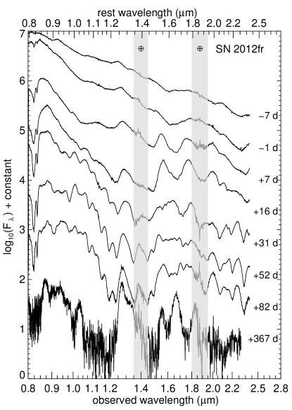
Figure 1: A sampling of NIR spectroscopic time evolution of the Type Ia SN 2012fr from pre-maximum through to transitional and nebular phases. All spectra shown were obtained with FIRE through the CSP-II NIR spectroscopy program. The phase relative to $B$-band maximum is labeled for each spectrum. The gray vertical bands mark the regions of the strongest telluric absorptions.

The top panel of Figure 2 shows that there are many spectra at all phases relevant for K-corrections and template building ($\lesssim 100$ days past maximum). For a few very nearby SNe Ia, the time series extends to the nebular phase, providing unique physical diagnostics which are described in Section 5. The bottom panel shows that the majority of SNe Ia have two spectra or more, providing the crucial time evolution information important for both explosion physics and K-correction studies. Figure 3 illustrates the characteristics of the SNe Ia observed in the NIR spectroscopy program. Nearly all of the SNe Ia are located within $z<0.05$. A few more distant objects have NIR spectra taken for classification only. The vast majority of the SNe Ia have optical light-curve follow up starting before maximum light, and the sample contains SNe Ia in the full range of light-curve shape parameters $s_{\mathrm{BV}}$ (Burns et al., 2014) and $\Delta m_{15}(B)$ (Phillips, 1993), determined using the updated version of SNooPy (Burns et al., 2011). Altogether, we obtained 661 NIR spectra of 157 SNe Ia. Within this sample, 451 NIR spectra of 90 SNe Ia are in the Physics sample with CSP-II light curve follow up.

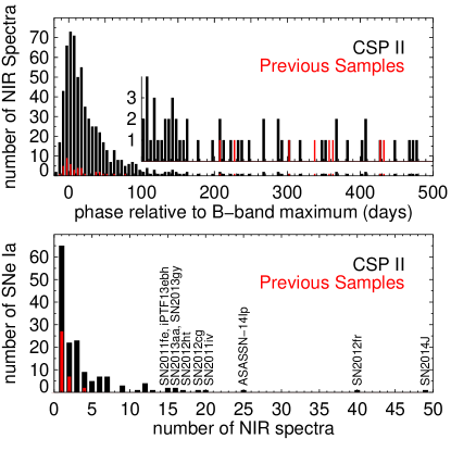
Figure 2: Number of NIR spectra at each epoch relative to $B$-band maximum (top panel) and number of SNe Ia with/without time-series observations (bottom panel). The inset of the top panel provides a zoomed-in view of the numbers at late times. SNe Ia with 15 NIR spectra or more have their names labeled in the bottom panel. The NIR spectra of SN 2011fe (Hsiao et al., 2013) and iPTF13ebh (Hsiao et al., 2015), and a subset of the NIR spectra of SN 2011iv (Gall et al., 2018), ASASSN-14lp and SN 2014J (Marion et al., 2015; Sand et al., 2016) were previously published.

Figure 3: Characteristics of the SNe Ia in the NIR spectroscopy program. The distributions in redshift, light curve follow up starting phase, $s_{BV}$, and $\Delta m_{15}(B)$ are shown in panels from left to right.

The list of SNe Ia for which we obtained NIR spectra is given in Table 1. Note that there are several objects which are only in the Cosmology sample. These objects are the most distant objects in our sample, and thus in most cases only have single-epoch low-S/N-ratio NIR spectra. Several objects belong to neither the Cosmology nor Physics samples for the following reasons. Some objects are of the peculiar SN 2002cx-like (e.g. Li et al., 2003; Foley et al., 2013) or “super-Chandrasekhar” (e.g. Howell et al., 2006) subtypes, which were excluded from both samples. Other objects do not have CSP-II follow up light curves either because they exploded between observing campaigns (e.g., SN 2012cg) or they are northern objects, as mentioned previously (e.g., SN 2011fe).

Time-series NIR spectroscopy of other SN types was also obtained, given that the existing samples are even smaller than that of SN Ia and the diagnostics in the NIR are just as powerful. Many NIR spectra of various SN types obtained by CSP-II have already been published in single-object papers: the rebrightening of SN 2009ip (Margutti et al., 2014), the Type IIb SN 2011hs (Bufano et al., 2014), the broad-lined Type Ic SN 2012ap (Milisavljevic et al., 2015), the Type Ib SN 2012au (Milisavljevic et al., 2013), the Type II SN 2012aw (Dall’Ora et al., 2014), the Type IIn SN 2012ca (Fox et al., 2015), the Type IIL SN 2013by (Valenti et al., 2015), the Type Ib/c SN 2013ge (Drout et al., 2016), as well as the SN 2002cx-like SN 2012Z (Stritzinger et al., 2015) and SN 2014ck (Tomasella et al., 2016). Note that SN 2012ca may be a SN Ia interacting with its surrounding circumstellar medium as noted by several studies (Inserra et al., 2014, 2016; Fox et al., 2015)

An atlas of the NIR spectra of supernovae of various types is plotted in Figure 4. The dominant ion species are labeled. The strong Ca II infrared triplet is present in all types of supernovae. Hydrogen Paschen and Brackett series are present in Type II supernovae. Note that Pa${\alpha}$ is located in the heavy telluric absorption between the $H$ and $K$ bands, therefore Pa${\beta}$ is often selected as the primary diagnostic in the NIR. The two strong NIR He I lines are present in Type IIb, IIn, and Ibn supernovae. One should be cognizant of the proximity between the He I $\lambda$1.0830 $\mu$m line and Pa${\gamma}$ when identifying features in the wavelength region near 1.1 $\mu$m. Multiple Mg II lines are dominant in early Type Ia and superluminous supernova (SLSN) NIR spectra. Table 2 shows the total number of NIR spectra taken by CSP-II according to SN type and instrument used. Note that these numbers include classification spectra that do not have accompanying light curves. We discuss our use of FIRE for classification of SN types further in Section 2. For every SN type, this data set of NIR spectra will at least double the existing published sample; and we hope, by opening the NIR window, the data set will further the understanding of each type of supernova.

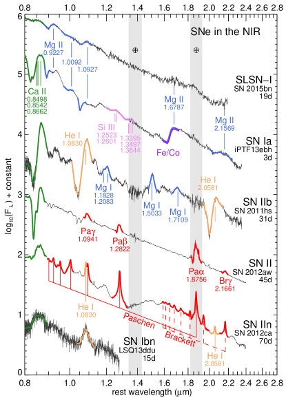
Figure 4: An atlas of NIR spectra of various SN types. The dominant ion species are labeled for comparison. The laboratory wavelengths are labeled in microns for reference and also marked on the figure as vertical lines. The supernova name and phase are labeled for each spectrum. The phases are relative to maximum light, except for that of SN 2012aw, which is relative to explosion. The gray vertical bands mark the regions of the strongest telluric absorptions. All spectra shown were taken with FIRE as part of the CSP-II NIR spectroscopy program. Spectra of iPTF13ebh (Hsiao et al., 2015), SN 2011hs (Bufano et al., 2014), SN 2012aw (Dall’Ora et al., 2014), and SN 2012ca (Fox et al., 2015) were published previously. FIRE spectra of the SLSN-I SN 2015bn and the Type Ibn LSQ13ddu are shown for the first time.

4 K-corrections

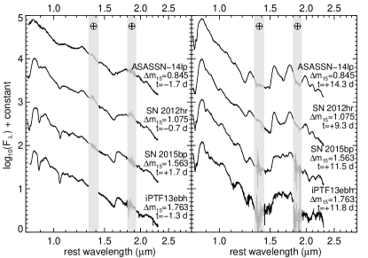
Figure 5: Comparison of SN Ia NIR spectra of various decline rate $\Delta m_{15}(B)$ values. The left and right panels show the spectra near maximum and $1-2$ weeks past maximum, respectively. The SN name, $\Delta m_{15}(B)$, and spectral phase are labeled for each spectrum. The gray vertical bands mark the regions of the strongest telluric absorptions. The spectral diversity in the NIR is strongly correlated with light-curve shape.

K-corrections account for the effect of cosmological expansion upon measured magnitudes (Oke & Sandage, 1968). As mentioned in the introduction, shifting SN Ia cosmology to the rest-frame NIR has the crucial advantages of largely circumventing the empirical width-luminosity relation and any uncertain dust reddening laws. This method is considered one of the most promising ways to reduce current SN Ia cosmology systematics. The potential of SNe Ia as standard candles in the NIR has been demonstrated in many studies (e.g., Krisciunas et al., 2004; Wood-Vasey et al., 2008; Folatelli et al., 2010; Barone-Nugent et al., 2012; Stanishev et al., 2018; Burns et al., 2018). Furthermore, all these studies utilized rudimentary K-corrections based on a small number of spectra. Any low-redshift experiment testing the efficacy of SNe Ia as standard candles in the NIR and any high-redshift experiment in the rest-frame NIR constraining the properties of dark energy will benefit from accurate knowledge of the diversity and time-evolution of NIR spectra.

Preliminary studies of NIR K-corrections yielded the promising result of a K-correction error from the diversity in spectral features of 0.04 mag at $z=0.08$ in the $Y$ band (Boldt et al., 2014), but studies of the other NIR bands were limited by poor telluric corrections. It is only feasible to obtain high S/N ratio NIR spectra for SNe Ia at $z\lesssim 0.03$. This redshift range does not allow for the sampling of the entire telluric-obscured regions. Furthermore, our CSP-II Cosmology sample for testing the efficacy of SN Ia cosmology in the NIR has a redshift range of $0.03\lesssim z\lesssim 0.1$. This means we are relying solely on the telluric-obscured region of our NIR spectroscopic sample to K-correct the NIR light curves of our Cosmology sample, again emphasizing the importance of telluric corrections. For our FIRE sample, the high-throughput prism mode allows for the collection of enough SN photons under the water vapor absorptions in most cases (see Section 2 for details).

Another key to successful K-corrections is our ability to predict the correct spectral energy distribution with only photometric information. It has been shown that even though there is substantial spectroscopic diversity in both the optical and NIR, defining a mean spectrum eliminates systematic errors and reduces the statistical errors to an acceptable level (Hsiao et al., 2007; Hsiao, 2009). There is also strong evidence that optical spectral features vary with decline rate (e.g., Nugent et al., 1995), and indications of the same behavior in the NIR (Hsiao et al., 2013). Figure 5 shows that $\Delta m_{15}(B)$ is a strong indicator of NIR spectroscopic diversity for both near- and post-maximum phases. For example, the strong Mg II $\lambda$1.0927$\mu$m absorption feature increases in strength as we go from slow to fast-declining SNe Ia (left panel of Figure 5). The most prominent feature in the NIR for SNe Ia, the $H$-band break near 1.5 $\mu$m, is shown quantitatively to correlate tightly with $\Delta m_{15}(B)$ and $s_{BV}$ (right panel of Figure 5; Hsiao et al., 2013; Hsiao et al., 2015). The accuracy of K-corrections can thus be further improved by characterizing the spectral variation with $\Delta m_{15}(B)$ or $s_{BV}$. Our large sample of NIR spectra will, for the first time, adequately fill the parameter space of wavelength (including telluric obscured regions), phase, and light-curve shape parameters.

5 Physics of SNe Ia

While the primary goal of the CSP-II NIR spectroscopy data set is to characterize SN Ia K-corrections in the NIR, the same data set is also a valuable resource for studying the physics and the progenitors of SNe Ia. The NIR spectral region has several unsaturated, strong and relatively isolated lines. Furthermore, optical and NIR spectra at the same phase probe completely different regions in the ejecta (Wheeler et al., 1998). Figure 6 shows comparison of spectral features of normal and peculiar SNe Ia in the SN 2002cx-like and the “super-Chandrasekhar” subtypes. In the optical, the spectral features between normal and peculiar SNe Ia are broadly similar. Indeed, that is why they are all classified as Type Ia. In the NIR, on the other hand, their spectral features are drastically different, revealing possible separate origins. Recent advances in the modeling of this wavelength region are also rapidly expanding the NIR tool set. We summarize some of these diagnostics here. More detailed analysis for each will be presented in forthcoming papers.

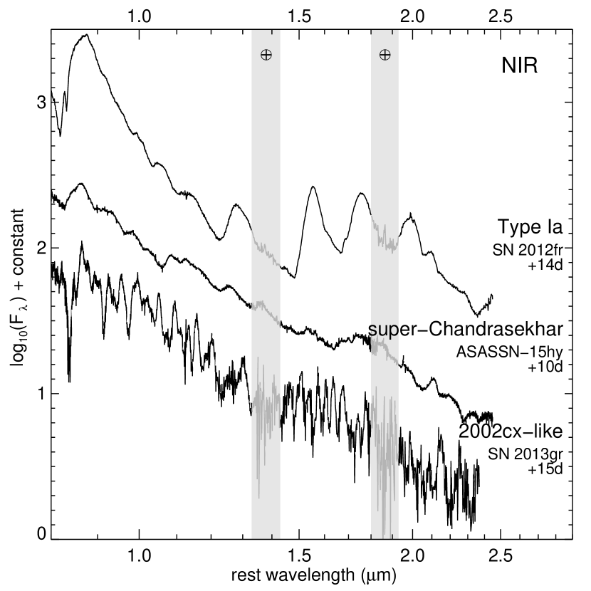
Figure 6: Comparison of spectral features of normal and peculiar SNe Ia. Left and right panels show spectra in the optical and NIR, respectively. In the right panel, the gray vertical bands mark the regions of the strongest telluric absorptions. In the optical, the spectral features between normal and peculiar SNe Ia are broadly similar. Indeed, that is why they are all classified as Type Ia. In the NIR, on the other hand, their spectral features are drastically different, revealing possible separate origins. The optical spectra of SNe 1994D (Ruiz-Lapuente et al., 1997), 2009dc (Taubenberger et al., 2011), and 2005hk (Phillips et al., 2007) were previously published. The GNIRS spectrum of ASASSN-15hy and FIRE spectra of SNe 2012fr and 2013gr were obtained as part of the CSP-II NIR spectroscopy program.

5.1 Unburned Material via C I $\lambda$1.0693 $\mu$m

The general consensus for the origin of a SN Ia is the thermonuclear explosion of a carbon-oxygen white dwarf (Hoyle & Fowler, 1960). Since oxygen is also produced from carbon burning, carbon provides the most direct probe of the primordial material from the progenitor white dwarf. The quantity, distribution and incidence of unburned carbon provides important constraints for explosion models. The Chandrasekhar-mass DDT scenario predicts nearly complete carbon burning for normal SNe Ia (Kasen et al., 2009) and increasing amounts of surviving carbon for fainter SNe Ia (Höflich et al., 2002). The pulsating class of DDT models also leaves large amounts of unburned carbon, even for normal objects (Hoeflich et al., 1995). On the other hand, unburned carbon is not expected to survive in the explosions of sub-Chandrasekhar mass white dwarfs, except for a small amount below the outer layer of iron-group elements produced during the surface helium detonation (e.g., Fink et al., 2010).

Until recently, the study of unburned material had mainly relied on the optical C II $\lambda$0.6580 $\mu$m line, which is marred by several selection biases. It is a weak spectral feature situated near the emission component of the strong Si II $\lambda$0.6355 $\mu$m P-Cygni profile, such that high-velocity carbon may be buried in the silicon absorption and measured velocities suffer from limb variation effects (Hoeflich, 1990). It also tends to fade rapidly after explosion, which makes obtaining a complete sample rather difficult. Surveys of large optical spectroscopic samples found that $20-30$% of pre-maximum spectra show C II signatures (Thomas et al., 2011; Parrent et al., 2011; Folatelli et al., 2012; Silverman & Filippenko, 2012).

In contrast to the weak and fast-fading nature of the optical C II $\lambda$0.6580 $\mu$m line, the NIR C I $\lambda$1.0693 $\mu$m line may be much stronger. Also, it increases in strength toward maximum light for normal-bright objects (Hsiao et al., 2013). The delayed onset of the NIR C I line may be a manifestation of the recombination from C II to C I as the ejecta expands and cools, and highlights the potential of the NIR C I line to secure more representative properties of unburned material in SNe Ia. With the aid of SYNAPPS (Thomas et al., 2011), the NIR C I feature has been identified in several SNe Ia with a large range of peak magnitudes (Figure 7; Hsiao et al., 2013; Hsiao et al., 2015; Marion et al., 2015). While the current number of NIR carbon detections is small, the incidence of carbon appears to be ubiquitous, with the fast-declining, fainter SNe Ia having the strongest C I lines. This preliminary result appears to contradict the claim of Blondin et al. (2017) that fast-declining faint SNe Ia result from the explosions of sub-Chandrasekhar-mass white dwarfs. However, more detailed analysis is needed to determine whether the small amount of unburned carbon beneath the surface iron-peak layer in sub-Chandrasekhar-mass models can produce the observed carbon features. With the CSP-II sample of $\sim 120$ pre-maximum NIR spectra of $\sim 50$ SNe Ia, we aim to characterize the properties of unburned material in SNe Ia in an unbiased fashion.

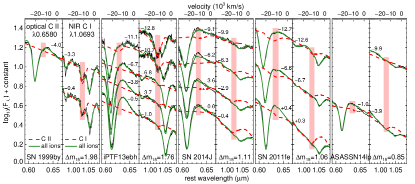
Figure 7: Comparison between the optical C II $\lambda$0.6580 $\mu$m and the NIR C I $\lambda$1.0693 $\mu$m lines of the five SNe Ia with C I detections. This plot is an expansion of Figure 10 in Hsiao et al. (2015) with the addition of the slow-declining ASASSN-14lp. The optical/NIR pair is selected such that the spectra are close in phase for each SN Ia. The phases relative to $B$ maximum are labeled. The velocity axes are plotted with respect to each carbon line. The SYNAPPS (Thomas et al., 2011) fits are plotted in green solid curves. We also plot the isolated influence from the carbon lines of the same fits in red dashed curves. The vertical pink bars provide guides to the locations of the carbon absorption troughs, or approximately where they would be if the features are indeed present. Except at the very early epoch of SN 2011fe, the NIR C I line is always stronger than the optical C II line.

In the sub-Chandrasekhar helium detonation scenario, unburned helium left over from the surface helium layer can potentially produce strong NIR He I $\lambda$1.0830 and $\lambda$2.0581 $\mu$m lines, as we have shown for other supernova types in Figure 4. Boyle et al. (2017) explored these features, and the possibility of confusion with the C I $\lambda$1.0693 $\mu$m line. This emphasizes the importance of identifying multiple lines of the same ion when searching for unburned carbon, as was done for SN 1999by (Höflich et al., 2002) and iPTF13ebh (Hsiao et al., 2015). Note that both of these objects are fast-declining, fainter SNe Ia, which tend to show the strongest C I lines.

5.2 Radioactive Nickel via $H$-band Break

A dramatic shift in the amount of line blanketing from iron-group elements takes place near 1.5 $\mu$m and produces the strong $H$-band break after maximum light (Wheeler et al., 1998). Observationally, SNe Ia are found to have uniform evolution of the $H$-band features. The $H$-band break appears at $\sim 3$ days past maximum and rapidly increases in strength as the feature formed by iron-peak elements becomes fully exposed at $\sim 12$ days past maximum. It then steadily decreases in strength at very similar rates for all SNe Ia out to approximately one month past maximum. The maximum size of the $H$-band break, when the iron-peak complex is fully exposed, is also found to correlate with the SN Ia light curve decline rate $\Delta m_{15}(B)$ (Hsiao et al., 2013).

The size and velocity shift of the $H$-band break probes the amount and distribution of radioactive ⁵⁶Ni, and the time evolution of the $H$-band break is related to the amount of intermediate-mass elements acting as the “shielding mass.” In the Chandrasekhar-mass DDT scenario, for example, there is an increasing amount of intermediate-mass elements produced with decreasing ⁵⁶Ni production; while for the sub-Chandrasekhar-mass He detonation scenario, the ⁵⁶Ni production increases with the total mass. Each scenario therefore produces a unique rate at which the $H$-band complex is exposed and a specific correlation between the strength of the $H$-band break and $\Delta m_{15}(B)$. CSP-II has gathered $\sim 300$ NIR spectra of $\sim 120$ SNe Ia between maximum light and $+30$ days. We aim to use this sample to confirm the strong correlation with decline rate discovered by Hsiao et al. (2013); Hsiao et al. (2015) with only ten SNe Ia, in addition to improving the measurements of the rate at which the $H$-band complex is exposed, which is currently poorly constrained.

5.3 Companion Signature via Pa${\beta}$ and He I

The nature of the companion star in the progenitor system is still a mystery. The collision between the SN Ia ejecta and the companion may produce detectable signatures that can be used to place constraints on the properties of the companion star (e.g., Kasen, 2010), although predictions on whether the signature is detectable may be model-dependent (Cumming et al., 1996). In particular, if the companion star has a hydrogen or helium-rich envelope in a single-degenerate system, the envelope is expected to be stripped away during the collision and be embedded deep within the low-velocity part of the expanding SN Ia ejecta (Marietta et al., 2000). This has been suggested to produce H${\alpha}$ in late-time spectra, beyond 200 days. So far, none has been detected in nearby SNe Ia (e.g., Mattila et al., 2005; Shappee et al., 2013; Sand et al., 2018). More recently, Maeda et al. (2014) suggested that NIR Pa${\beta}$ companion signature is potentially much stronger than H${\alpha}$, and appears much earlier. The strong NIR He I lines can also be easily detected (Botyánszki et al., 2018). These desirable properties could lead to the first detection of embedded hydrogen or helium stripped from the companion star or at least place stronger constraints on its absence. We published the first searches for the Pa${\beta}$ emission in the NIR. Although these were also non-detections, they placed upper limits of $<0.1$ $M_{\sun}$ of stripped hydrogen from the companion stars of SNe 2014J (Sand et al., 2016) and 2017cbv (Hosseinzadeh et al., 2017).

Two main challenges for the detection of these so-far elusive hydrogen lines are: 1) viewing angle effects and 2) diversity of the SN Ia feature underneath the hydrogen emissions, both requiring a statistically significant sample. The CSP-II data set with $\sim 100$ NIR spectra of $\sim 50$ SNe Ia between one and two months past maximum currently is the best data set for such a study.

5.4 Neutron Content via [Ni II] 1.939 $\mu$m

Recent theoretical studies of SNe Ia undergoing the transition from the photospheric to nebular phase identified a strong NIR emission feature as [Ni II] $\lambda$1.939 $\mu$m (Friesen et al., 2014; Wilk et al., 2018), although this identification had been disputed by Blondin et al. (2015). At such late phases, all of the radioactive ⁵⁶Ni has decayed into ⁵⁶Co. If the observed line is indeed attributed to [Ni II], it must then be produced by the stable isotope ⁵⁸Ni. Furthermore, since we are likely probing the neutron content in the inner region at these late phases, the detection of [Ni II] features would indicate high-density burning (Thielemann et al., 1986; Iwamoto et al., 1999) and may be less sensitive to the metallicity of the progenitor (Höflich et al., 1998; Timmes et al., 2003) or the neutronization in the simmering phase (Piro & Bildsten, 2008). High-density burning is a hallmark of Chandrasekhar-mass DDT models, while sub-Chandrasekhar explosion models tend to underproduce stable neutron-rich elements (Seitenzahl et al., 2013).

Spectra in the NIR obtained during the transition to nebular phase are still quite rare. Furthermore, the [Ni II] $\lambda$1.939 $\mu$m line is close to the strong telluric water vapor absorptions between $H$ and $K$ bands. Friesen et al. (2014) gathered four NIR spectra from the literature and two new observations of SN 2014J between 50 and 100 days past explosion. Only the two NIR spectra of SN 2014J had adequate wavelength coverage, telluric correction, and S/N ratio to detect the presence of this feature. The feature was also reported in the NIR nebular spectra of SN 2014J obtained by Dhawan et al. (2018). With the CSP-II sample of $\sim 100$ transitional to nebular phase NIR spectra of $\sim 40$ SNe Ia, we aim to analyze the diversity in the properties of this feature. Figure 1 shows an example of our time-series data, taken of SN 2012fr. The feature reported by Friesen et al. (2014) was indeed also present in SN 2012fr and evolved to be its strongest feature in the $K$ band during the transitional phase (+82 days past $B$ maximum in Figure 1). By the nebular phase, the feature became much weaker, and our nebular spectrum at +367 days unfortunately did not have a high enough S/N ratio to confirm the presence of this feature. Further study on the modeling side is also planned to secure the identification of this line.

5.5 Central Density and Magnetic Field via [Fe II] 1.644 $\mu$m

Nebular phase observations of line profiles can reveal the isotopic structure of the inner region. In particular, the forbidden [Fe II] 1.644 $\mu$m line is ideal for such studies, since it is strong and unblended. It can be used to measure the properties of the progenitor system and explosion, such as asphericity, initial central density, and magnetic field (Penney & Hoeflich, 2014; Diamond et al., 2015, 2018). Up to 200 days past explosion, the line profile can be used to analyze the overall chemical and density structure of the exploding white dwarf without considering the magnetic field, since the energy deposition by gamma ray photons dominates. Measurements of the central density can lead us to the accretion history of the pre-explosion white dwarf (Nomoto et al., 1984) and the amount of stable ⁵⁸Ni produced (Höflich et al., 2006). Note that updated electron capture rates (e.g., Brachwitz et al., 2000) no longer yield enough stable iron group elements to produce the “flat-top” profiles emphasized by Maguire et al. (2018), except in the most extreme cases. Rather, increasing central density widens the line width of the [Fe II] 1.644 $\mu$m line and the effects can be measured with moderate S/N ratio nebular spectra (Diamond et al., 2015, 2018). Going to even later phases, beyond one year past explosion, the time evolution of the line profile is sensitive to positron transport effects. The escape probability of the positrons, which directly influences the width of the [Fe II] line, depends strongly on the size and the morphology of the magnetic fields.

For the Chandrasekhar-mass DDT scenario, 3D hydrodynamical simulations consistently predict large-scale mixing of the ejecta due to Rayleigh-Taylor instabilities during the deflagration burning phase (Röpke et al., 2006), producing results which are inconsistent with observations. Recently, Hristov et al. (2018) found that the magnetic field plays an important role during this burning phase. Their magnetohydrodynamical study showed increasing suppression of the instabilities starting at $\sim 10^{9}$ G. Such magnetic fields may be generated during the pre-explosive carbon-simmering phase of Chandrasekhar-mass explosions (Piro & Chang, 2008). Current measurements based on a handful of NIR nebular spectra of nearby SNe Ia indicated relatively high central densities and high magnetic fields (e.g., Penney & Hoeflich, 2014; Diamond et al., 2015). We are extending the analysis to the CSP-II sample of $\sim 20$ NIR spectra of seven SNe Ia at phases beyond 200 days past explosion. Meanwhile, ongoing programs at Gemini and LCO, as part of CSP-II, continue to monitor the time evolution of the [Fe II] line profile of nearby SNe Ia.

6 Summary

This paper presents an introduction to the CSP-II NIR spectroscopy program, which we carried out from 2011 to 2015. This project represents an important step for any current and future SN Ia cosmological experiments based on the rest-frame NIR. These experiments have been shown to reduce errors by effectively circumventing the uncertain dust laws and empirical width-luminosity relation. The data set collected is unique in its large sample size, time-series observations, complementary light-curve and optical spectroscopic observations, and improvement in the telluric regions. Such a sample makes it possible to quantify the representative NIR spectroscopic time evolution and diversity of SNe Ia, allowing NIR cosmological experiments to reach their true potential. By exploring the NIR wavelength window, many diagnostics for the explosion mechanisms and the progenitor systems of SNe Ia also become available. Understanding the origins of these events represents a second and independent way to reduce systematic errors in SN Ia cosmology. While our focus is on normal SNe Ia for cosmological studies, comparisons of NIR spectroscopic features between normal and peculiar SNe Ia (Figure 6), and between supernovae of various types (Figure 4), highlight the identifying features and offer clues to the origins of these events.

Table 1: Summary of CSP-II NIR spectroscopy of SNe Ia

SN Name	Number of NIR spectra	Sample	$z_{\rm{helio}}$	Classification by FIRE
ASASSN-13ar (SN 2013dl)	3		0.0178
ASASSN-13av	3		0.0173
ASASSN-14ad	6	P	0.0264
ASASSN-14eu	1		0.0227
ASASSN-14hp	1	C	0.0389
ASASSN-14hu	2	P	0.0216
ASASSN-14jc	1	P	0.0113
ASASSN-14jg	4	P	0.0148
ASASSN-14lo	1	P	0.0199
ASASSN-14lp	25	P	0.0051
ASASSN-14lq	1	P	0.0262
ASASSN-14lw	3	P	0.0209	ATel 6832
ASASSN-14me	3	P	0.018
ASASSN-14mw	3	C,P	0.0274
ASASSN-14my	4	P	0.0205
ASASSN-15aj	2	P	0.0109
ASASSN-15as	2	C,P	0.0286	ATel 6920
ASASSN-15ba	2	P	0.0231
ASASSN-15be	2	P	0.0219
ASASSN-15bm	3	P	0.0208
ASASSN-15cd	1	C	0.0344
ASASSN-15eb	1	P	0.0165
ASASSN-15fr	1	C,P	0.0334
ASASSN-15fy	1		0.025	ATel 7354
ASASSN-15ga	3	P	0.0066
ASASSN-15go	1	P	0.0189
ASASSN-15gr	1	P	0.0243
ASASSN-15hf	3	P	0.0062
ASASSN-15hx	6	P	0.008
ASASSN-15hy	6		0.025
CSS110414:145909+071804 (SN 2011cg)	1		0.020
CSS110504:101800-023241 (SN 2011ci)	1		0.0472
CSS110604:130707-011044 (SN 2011dj)	1		0.0185
CSS111231:145323+025743 (SN 2011jt)	1	P	0.0278
CSS120224:145405+220541 (SN 2012aq)	1	C	0.052
CSS120301:162036-102738 (SN 2012ar)	6	C,P	0.0283	CBET 3041
CSS121114:090202+101800	1	C	0.0371
SSS130304:114445-203141 (SN 2013ao)	6		0.0435
CSS130315:114144-171348	1		0.050
CSS130614:233746+144237 (SN 2013dn)	3		0.0562
CSS131225:030144-092044	1		0.040	ATel 5702
CSS150214:140955+173155 (SN 2015bo)	1	P	0.0162
SNhunt37 (SN 2011ae)	1		0.0060
SNhunt46 (SN 2011be)	1		0.0340
SNhunt177 (SN 2013az)	1	C	0.0373	CBET 3457, ATel 4935
SNhunt178 (SN 2013bc)	1	P	0.0225	CBET 3468, ATel 4948
SNhunt188 (SN 2013bz)	1	P	0.0192
SNhunt224 (SN 2013hs)	1		0.0195	CBET 3770, ATel 5702
SNhunt229 (SN 2014D)	2	P	0.0082	CBET 3778
SNhunt281 (SN 2015bp)	9	P	0.0041
KISS15n (SN 2015M)	1	P	0.0231
LSQ11bk	2	C	0.0403
LSQ11ot	3	C,P	0.0273
LSQ11pn	1	C,P	0.0327
LSQ12bia	1		0.053
LSQ12btn	2	C	0.0542
LSQ12cpf	2		0.0286
LSQ12dbr	1		0.020
LSQ12frx	1		0.030
LSQ12fuk	2	P	0.0206
LSQ12fxd	7	C,P	0.0312
LSQ12gdj	5	C,P	0.0303
LSQ12hzj	1	C,P	0.0334
LSQ13pf	1	C	0.0861	ATel 4916
LSQ13ry	2	C,P	0.0299	ATel 4935
LSQ13aiz (SN 2013cs)	3	P	0.0092
LSQ13dsm	3	C	0.0424	ATel 5714
LSQ14xi	1	C	0.0508
LSQ14ajn (SN 2014ah)	2	P	0.0210
LSQ14dsu	1		0.0196
LSQ15aae	1	C	0.0516
LSQ15adm	1		0.0723
MASTER OT J030559.89+043238.2	3	P	0.0282
OGLE-2014-SN-019	1	C	0.0359
PS1-14ra	3	C,P	0.0281
PS15sv	3	C,P	0.0333
PSN J13471211-2422171	1	P	0.0199
PTF11bju	1		0.0323
PTF11kly (SN 2011fe)	15		0.0008
PTF11pbp (SN 2011hb)	3	C,P	0.0289
PTF11qnr	3	P	0.0162
PTF12ena	1		0.0166
iPTF13asv	1		0.035
iPTF13dge	1		0.0159
iPTF13duj	4	P	0.0170
iPTF13dym	1	C	0.0422
iPTF13dzm	1		0.0158
iPTF13ebh	15	P	0.0133	ATel 5580
iPTF14aaf	1		0.0589
iPTF14abh	1		0.0237
iPTF14ans	1		0.0318
iPTF14bdn	1		0.0156
iPTF14sz	1		0.0288
iPTF14w	7	P	0.0189
iPTF14yw (SN 2014aa)	4	P	0.0170
iPTF14yy	1	C	0.0431
iPTF14fpg (SN 2014dk)	4	C,P	0.0319
iPTF15ku	5		0.0282
ROTSE3 J123935.1+163512 (SN 2012G)	2	P	0.0266
SN 2011at	2		0.0068
SN 2011bf	2		0.0167
SN 2011ce	3		0.0086
SN 2011di	1		0.0147
SN 2011iv	20	P	0.0065
SN 2011iy	13	P	0.0043
SN 2011jh	11	P	0.0078
SN 2011jl	2		0.0100
SN 2012E	4	P	0.0203
SN 2012U	1	P	0.0197
SN 2012Z	12		0.0071
SN 2012ah	1	P	0.0124
SN 2012bl	9	P	0.0187
SN 2012bo	7	P	0.0254
SN 2012cg	19		0.0015	ATel 4119
SN 2012db	1		0.0193
SN 2012fr	40	P	0.0055
SN 2012gm	2	P	0.0148
SN 2012hd	5	P	0.0120
SN 2012hr	12	P	0.0076	CBET 3346, ATel 4663
SN 2012ht	17	P	0.0036
SN 2012id	3	P	0.0157
SN 2012ij	3	P	0.0110
SN 2013E	12	P	0.0094
SN 2013H	4	P	0.0155
SN 2013M	3	C,P	0.0350
SN 2013N	1		0.0256
SN 2013U	2	C,P	0.0345
SN 2013aa	16	P	0.0040
SN 2013aj	9	P	0.0091
SN 2013ay	2	P	0.0157	CBET 3456, ATel 4935
SN 2013cg	1	P	0.0080
SN 2013ct	7	P	0.0038	CBET 3539, ATel 5081
SN 2013dh	2		0.0134
SN 2013dt	3		0.0241
SN 2013fb	1		0.0170
SN 2013fy	6	C,P	0.0309
SN 2013fz	7	P	0.0206
SN 2013gr	12		0.0074	CBET 3733, ATel 5612
SN 2013gv	4	C,P	0.0341
SN 2013gy	16	P	0.0140
SN 2013hh	7	P	0.0130
SN 2013hl	1		0.0262	CBET 3759, ATel 5664
SN 2013hn	4	P	0.0151
SN 2014I	5	C,P	0.0300
SN 2014J	49		0.0007
SN 2014Z	1	P	0.0213	CBET 3822, ATel 5959
SN 2014ao	5	P	0.0141
SN 2014at	2	C,P	0.0322
SN 2014ba	2	P	0.0058
SN 2014cd	1		0.0206
SN 2014ck	7		0.0050
SN 2014cz	1		0.0260	CBET 3965, ATel 6442
SN 2014du	1	C,P	0.0325
SN 2014eg	1	P	0.0186
SN 2014ek	1		0.0231
SN 2015F	6	P	0.0049
SN 2015H	3		0.0125

Table 2: Number of NIR spectra by instrument and SN type

Telecope	Instrument	Ia	2002cx-like	Ibc	II	IIn	SLSN	Others	Total
Magellan Baade	FIRE	450	27	97	79	35	9	4	701
Magellan Clay	MMIRS	7	1	2	1	0	0	1	12
Gemini North	GNIRS	63	7	0	0	0	0	0	70
Gemini South	FLAMINGOS2	17	0	0	1	0	0	0	18
IRTF	SpeX	40	1	6	9	2	0	0	58
VLT	ISAAC	8	4	0	0	0	0	0	12
NTT	SofI	4	1	2	0	0	0	0	7
Mt Abu	NICS	31	0	0	0	0	0	0	31
total spectra		620	41	107	90	37	9	5	909
total SNe		149	8	42	31	12	5	2	249

References

- Baltay et al. (2013) Baltay, C., et al. 2013, Publications of the Astronomical Society of the Pacific, 125, 683
- Barone-Nugent et al. (2012) Barone-Nugent, R. L., et al. 2012, Monthly Notices of the Royal Astronomical Society, 425, 1007
- Betoule et al. (2014) Betoule, M., et al. 2014, Astronomy and Astrophysics, 568, A22
- Blondin et al. (2015) Blondin, S., Dessart, L., & Hillier, D. J. 2015, Monthly Notices of the Royal Astronomical Society, 448, 2766
- Blondin et al. (2017) Blondin, S., et al. 2017, Monthly Notices of the Royal Astronomical Society, 470, 157
- Blondin & Tonry (2007) Blondin, S., & Tonry, J. L. 2007, The Astrophysical Journal, 666, 1024
- Boldt et al. (2014) Boldt, L. N., et al. 2014, Publications of the Astronomical Society of the Pacific, 126, 324
- Botyánszki et al. (2018) Botyánszki, J., Kasen, D., & Plewa, T. 2018, The Astrophysical Journal, 852, L6
- Boyle et al. (2017) Boyle, A., et al. 2017, Astronomy and Astrophysics, 599, A46
- Brachwitz et al. (2000) Brachwitz, F., et al. 2000, The Astrophysical Journal, 536, 934
- Bufano et al. (2014) Bufano, F., et al. 2014, Monthly Notices of the Royal Astronomical Society, 439, 1807
- Burns et al. (2014) Burns, C. R., et al. 2014, The Astrophysical Journal, 789, 32
- Burns et al. (2011) Burns, C. R., et al. 2011, The Astronomical Journal, 141, 19
- Burns et al. (2018) Burns, C. R., et al. 2018, ArXiv e-prints, arXiv:1809.06381
- Conley et al. (2011) Conley, A., et al. 2011, The Astrophysical Journal Supplement Series, 192, 1
- Contreras et al. (2010) Contreras, C., et al. 2010, The Astronomical Journal, 139, 519
- Contreras et al. (2018) Contreras, C., et al. 2018, The Astrophysical Journal, 859, 24
- Cumming et al. (1996) Cumming, R. J., et al. 1996, Monthly Notices of the Royal Astronomical Society, 283, 1355
- Cushing et al. (2004) Cushing, M. C., Vacca, W. D., & Rayner, J. T. 2004, Publications of the Astronomical Society of the Pacific, 116, 362
- Dall’Ora et al. (2014) Dall’Ora, M., et al. 2014, The Astrophysical Journal, 787, 139
- Dhawan et al. (2018) Dhawan, S., et al. 2018, ArXiv e-prints, arXiv:1805.02420
- Diamond et al. (2018) Diamond, T. R., et al. 2018, The Astrophysical Journal, 861, 119
- Diamond et al. (2015) Diamond, T. R., Hoeflich, P., & Gerardy, C. L. 2015, The Astrophysical Journal, 806, 107
- Drout et al. (2016) Drout, M. R., et al. 2016, The Astrophysical Journal, 821, 57
- Eikenberry et al. (2008) Eikenberry, S., et al. 2008, Ground-based and Airborne Instrumentation for Astronomy II, 7014, 70140V
- Elias et al. (2006) Elias, J. H., et al. 2006, Society of Photo-Optical Instrumentation Engineers (SPIE) Conference Series, 6269, 62694C
- Filippenko (1982) Filippenko, A. V. 1982, Publications of the Astronomical Society of the Pacific, 94, 715
- Fink et al. (2010) Fink, M., et al. 2010, Astronomy and Astrophysics, 514, A53
- Folatelli et al. (2010) Folatelli, G., et al. 2010, The Astronomical Journal, 139, 120
- Folatelli et al. (2012) Folatelli, G., et al. 2012, The Astrophysical Journal, 745, 74
- Foley et al. (2013) Foley, R. J., et al. 2013, The Astrophysical Journal, 767, 57
- Fox et al. (2015) Fox, O. D., et al. 2015, Monthly Notices of the Royal Astronomical Society, 447, 772
- Freedman et al. (2009) Freedman, W. L., et al. 2009, The Astrophysical Journal, 704, 1036
- Friesen et al. (2014) Friesen, B., et al. 2014, The Astrophysical Journal, 792, 120
- Gall et al. (2018) Gall, C., et al. 2018, Astronomy and Astrophysics, 611, A58
- González-Martín et al. (2013) González-Martín, O., et al. 2013, Astronomy and Astrophysics, 553, A35
- Hachinger et al. (2008) Hachinger, S., et al. 2008, Monthly Notices of the Royal Astronomical Society, 389, 1087
- Hamuy et al. (2006) Hamuy, M., et al. 2006, Publications of the Astronomical Society of the Pacific, 118, 2
- Harutyunyan et al. (2008) Harutyunyan, A. H., et al. 2008, Astronomy and Astrophysics, 488, 383
- Hoeflich (1990) Hoeflich, P. 1990, Astronomy and Astrophysics, 229, 191
- Höflich (1995) Höflich, P. 1995, The Astrophysical Journal, 443, 89
- Hoeflich et al. (1995) Hoeflich, P., Khokhlov, A. M., & Wheeler, J. C. 1995, The Astrophysical Journal, 444, 831
- Höflich et al. (1998) Höflich, P., Wheeler, J. C., & Thielemann, F. K. 1998, The Astrophysical Journal, 495, 617
- Höflich et al. (2002) Höflich, P., et al. 2002, The Astrophysical Journal, 568, 791
- Höflich et al. (2006) Höflich, P., et al. 2006, New Astronomy Reviews, 50, 470
- Hoeflich et al. (2017) Hoeflich, P., et al. 2017, The Astrophysical Journal, 846, 58
- Horne (1986) Horne, K. 1986, Publications of the Astronomical Society of the Pacific, 98, 609
- Hosseinzadeh et al. (2017) Hosseinzadeh, G., et al. 2017, The Astrophysical Journal, 845, L11
- Howell et al. (2005) Howell, D. A., et al. 2005, The Astrophysical Journal, 634, 1190
- Howell et al. (2006) Howell, D. A., et al. 2006, Nature, 443, 308
- Hoyle & Fowler (1960) Hoyle, F., & Fowler, W. A. 1960, The Astrophysical Journal, 132, 565
- Hristov et al. (2018) Hristov, B., et al. 2018, The Astrophysical Journal, 858, 13
- Hsiao (2009) Hsiao, E. Y. 2009, Ph.D. Thesis, University of Victoria
- Hsiao et al. (2007) Hsiao, E. Y., et al. 2007, The Astrophysical Journal, 663, 1187
- Hsiao et al. (2013) Hsiao, E. Y., et al. 2013, The Astrophysical Journal, 766, 72
- Hsiao et al. (2015) Hsiao, E. Y., et al. 2015, Astronomy and Astrophysics, 578, A9
- Iben & Tutukov (1984) Iben, I., Jr., & Tutukov, A. V. 1984, The Astrophysical Journal Supplement Series, 54, 335
- Inserra et al. (2014) Inserra, C., et al. 2014, Monthly Notices of the Royal Astronomical Society, 437, L51
- Inserra et al. (2016) Inserra, C., et al. 2016, Monthly Notices of the Royal Astronomical Society, 459, 2721
- Iwamoto et al. (1999) Iwamoto, K., et al. 1999, The Astrophysical Journal Supplement Series, 125, 439
- Kasen et al. (2009) Kasen, D., Röpke, F. K., & Woosley, S. E. 2009, Nature, 460, 869
- Kasen (2006) Kasen, D. 2006, The Astrophysical Journal, 649, 939
- Kasen (2010) Kasen, D. 2010, The Astrophysical Journal, 708, 1025
- Kattner et al. (2012) Kattner, S., et al. 2012, Publications of the Astronomical Society of the Pacific, 124, 114
- Kelson (2003) Kelson, D. D. 2003, Publications of the Astronomical Society of the Pacific, 115, 688
- Khokhlov (1991) Khokhlov, A. M. 1991, Astronomy and Astrophysics, 245, 114
- Krisciunas et al. (2017) Krisciunas, K., et al. 2017, The Astronomical Journal, 154, 211
- Krisciunas et al. (2004) Krisciunas, K., Phillips, M. M., & Suntzeff, N. B. 2004, The Astrophysical Journal, 602, L81
- Law et al. (2009) Law, N. M., et al. 2009, Publications of the Astronomical Society of the Pacific, 121, 1395
- Li et al. (2003) Li, W., et al. 2003, Publications of the Astronomical Society of the Pacific, 115, 453
- Maeda et al. (2014) Maeda, K., Kutsuna, M., & Shigeyama, T. 2014, The Astrophysical Journal, 794, 37
- Maguire et al. (2018) Maguire, K., et al. 2018, Monthly Notices of the Royal Astronomical Society, 477, 3567
- Mandel et al. (2011) Mandel, K. S., Narayan, G., & Kirshner, R. P. 2011, The Astrophysical Journal, 731, 120
- Margutti et al. (2014) Margutti, R., et al. 2014, The Astrophysical Journal, 780, 21
- Marietta et al. (2000) Marietta, E., Burrows, A., & Fryxell, B. 2000, The Astrophysical Journal Supplement Series, 128, 615
- Marion et al. (2009) Marion, G. H., et al. 2009, The Astronomical Journal, 138, 727
- Marion et al. (2015) Marion, G. H., et al. 2015, The Astrophysical Journal, 798, 39
- Mattila et al. (2005) Mattila, S., et al. 2005, Astronomy and Astrophysics, 443, 649
- Milisavljevic et al. (2013) Milisavljevic, D., et al. 2013, The Astrophysical Journal, 770, L38
- Milisavljevic et al. (2015) Milisavljevic, D., et al. 2015, The Astrophysical Journal, 799, 51
- Nomoto (1982) Nomoto, K. 1982, The Astrophysical Journal, 253, 798
- Nomoto et al. (1984) Nomoto, K., Thielemann, F.-K., & Yokoi, K. 1984, The Astrophysical Journal, 286, 644
- Nugent et al. (1995) Nugent, P., et al. 1995, The Astrophysical Journal, 455, L147
- Oke & Sandage (1968) Oke, J. B., & Sandage, A. 1968, The Astrophysical Journal, 154, 21
- Parrent et al. (2011) Parrent, J. T., et al. 2011, The Astrophysical Journal, 732, 30
- Penney & Hoeflich (2014) Penney, R., & Hoeflich, P. 2014, The Astrophysical Journal, 795, 84
- Perlmutter et al. (1999) Perlmutter, S., et al. 1999, The Astrophysical Journal, 517, 565
- Persson et al. (2013) Persson, S. E., et al. 2013, Publications of the Astronomical Society of the Pacific, 125, 654
- Phillips (1993) Phillips, M. M. 1993, The Astrophysical Journal, 413, L105
- Phillips et al. (2007) Phillips, M. M., et al. 2007, Publications of the Astronomical Society of the Pacific, 119, 360
- Phillips et al. (2018) Phillips, M. M., et al. 2018, Publications of the Astronomical Society of the Pacific, submitted
- Piro & Bildsten (2008) Piro, A. L., & Bildsten, L. 2008, The Astrophysical Journal, 673, 1009
- Piro & Chang (2008) Piro, A. L., & Chang, P. 2008, The Astrophysical Journal, 678, 1158
- Röpke et al. (2006) Röpke, F. K., et al. 2006, Astronomy and Astrophysics, 453, 203
- Rayner et al. (2003) Rayner, J. T., et al. 2003, Publications of the Astronomical Society of the Pacific, 115, 362
- Riess et al. (1998) Riess, A. G., et al. 1998, The Astronomical Journal, 116, 1009
- Ruiz-Lapuente et al. (1997) Ruiz-Lapuente, P., Canal, R., & Isern, J. 1997, NATO Advanced Science Institutes (ASI) Series C, 486,
- Sand et al. (2016) Sand, D. J., et al. 2016, The Astrophysical Journal, 822, L16
- Sand et al. (2018) Sand, D. J., et al. 2018, The Astrophysical Journal, 863, 24
- Scolnic et al. (2018) Scolnic, D. M., et al. 2018, The Astrophysical Journal, 859, 101
- Seitenzahl et al. (2013) Seitenzahl, I. R., et al. 2013, Astronomy and Astrophysics, 559, L5
- Shappee et al. (2013) Shappee, B. J., et al. 2013, The Astrophysical Journal, 762, L5
- Silverman et al. (2012) Silverman, J. M., et al. 2012, Monthly Notices of the Royal Astronomical Society, 425, 1789
- Silverman & Filippenko (2012) Silverman, J. M., & Filippenko, A. V. 2012, Monthly Notices of the Royal Astronomical Society, 425, 1917
- Simcoe et al. (2013) Simcoe, R. A., et al. 2013, Publications of the Astronomical Society of the Pacific, 125, 270
- Stanishev et al. (2018) Stanishev, V., et al. 2018, Astronomy and Astrophysics, 615, A45
- Stritzinger et al. (2011) Stritzinger, M. D., et al. 2011, The Astronomical Journal, 142, 156
- Stritzinger et al. (2015) Stritzinger, M. D., et al. 2015, Astronomy and Astrophysics, 573, A2
- Stritzinger et al. (2018) Stritzinger, M. D., et al. 2018, Astronomy and Astrophysics, 609, A134
- Suzuki et al. (2012) Suzuki, N., et al. 2012, The Astrophysical Journal, 746, 85
- Taubenberger et al. (2011) Taubenberger, S., et al. 2011, Monthly Notices of the Royal Astronomical Society, 412, 2735
- Thielemann et al. (1986) Thielemann, F.-K., Nomoto, K., & Yokoi, K. 1986, Astronomy and Astrophysics, 158, 17
- Thomas et al. (2011) Thomas, R. C., et al. 2011, The Astrophysical Journal, 743, 27
- Thomas et al. (2011) Thomas, R. C., Nugent, P. E., & Meza, J. C. 2011, Publications of the Astronomical Society of the Pacific, 123, 237
- Timmes et al. (2003) Timmes, F. X., Brown, E. F., & Truran, J. W. 2003, The Astrophysical Journal, 590, L83
- Tomasella et al. (2016) Tomasella, L., et al. 2016, Monthly Notices of the Royal Astronomical Society, 459, 1018
- Vacca et al. (2003) Vacca, W. D., Cushing, M. C., & Rayner, J. T. 2003, Publications of the Astronomical Society of the Pacific, 115, 389
- Valenti et al. (2015) Valenti, S., et al. 2015, Monthly Notices of the Royal Astronomical Society, 448, 2608
- Webbink (1984) Webbink, R. F. 1984, The Astrophysical Journal, 277, 355
- Wheeler et al. (1998) Wheeler, J. C., et al. 1998, The Astrophysical Journal, 496, 908
- Whelan & Iben (1973) Whelan, J., & Iben, I., Jr. 1973, The Astrophysical Journal, 186, 1007
- Wilk et al. (2018) Wilk, K. D., Hillier, D. J., & Dessart, L. 2018, Monthly Notices of the Royal Astronomical Society, 474, 3187
- Wood-Vasey et al. (2008) Wood-Vasey, W. M., et al. 2008, The Astrophysical Journal, 689, 377