Dependency of halo concentration on mass, redshift and fossilness in Magneticum hydrodynamic simulations

Abstract

We study the dependency of the concentration on mass and redshift using three large N-body cosmological hydrodynamic simulations carried out by the Magneticum project. We constrain the slope of the mass-concentration relation with an unprecedented mass range for hydrodynamic simulations and find a negative trend on the mass-concentration plane and a slightly negative redshift dependency, in agreement with observations and other numerical works. We also show how the concentration correlates with the fossil parameter, defined as the stellar mass ratio between the central galaxy and the most massive satellite, in agreement with observations. We find that haloes with high fossil parameter have systematically higher concentration and investigate the cause in two different ways. First we study the evolution of haloes that lives unperturbed for a long period of time, where we find that the internal region keeps accreting satellites as the fossil parameter increases and the scale radius decreases (which increases the concentration). We also study the dependency of the concentration on the virial ratio and the energy term from the surface pressure $E_{s}$. We conclude that fossil objects have higher concentration because they are dynamically relaxed, with no in-fall/out-fall material and had time to accrete their satellites.

1 Introduction

Most density profiles of dark matter haloes from both simulations and observations can be described using a Navarro Frank and White (NFW) profile (Navarro et al. (1996, 1997), see Borgani & Kravtsov (2011) for a review). Such density profile is modelled as a function of the radial distance $r$ as:

$$\rho\left(r\right)=\frac{\rho_{0}}{\frac{r}{r_{s}}\left(1+\frac{r}{r_{s}}\right)^{2}},$$

where $r_{s}$ is a scale radius separating the internal and the external regions, and $\rho_{0}$ is four times the density at $r=r_{s}$.

As haloes do not have well defined boundaries, the virial radius $R_{vir}$ is assumed to be the radius at which the density of the halo is the one of a theoretical virialised spherical overdensity in an expanding universe. The density threshold is represented as $\Delta_{vir}\rho_{crit}.$ Here $\rho_{crit}$ is the critical density $\rho_{crit}\equiv 3H^{2}/4\pi G$ and $\Delta_{vir}$ is a parameter that depends on cosmology. For instance, $\Delta_{vir}\approx 178$ in an Einstein de Sitter cosmology (see Naderi et al. (2015) for a review). More generally, in the literature, people prefer to make use of radii definitions that are independent of cosmology and refer to $R_{\Delta}$ as the radius that includes an over-density of $\Delta\cdot\rho_{crit}.$ In the following analysis, we use both $\Delta={200}$ and $\Delta={500}$ and the corresponding radii $R_{200}$ and $R_{500}$.

The concentration $c_{\Delta}$ is defined as $c_{\Delta}\equiv R_{\Delta}/r_{s}$ and quantifies how wide is the internal region of the cluster, compared to its radius. Bullock et al. (2001) is a pioneering theoretical work devoted to the study of the concentration in a $\Lambda CDM$ universe. Their toy model based on an isolated spherical over-density, whose scale factor $a$ at the collapse time is $a_{c},$ predicts a concentration $c\propto a/a_{c},$ where the proportionality constant is universal for all haloes.

Various literature works make a fit of the concentration as a power law of the halo mass and redshift. They mainly found a very low dependency of concentration on redshift and a slow but steady decrease of the concentration with mass (see e.g. Dutton & Macciò, 2014; Merten et al., 2015). In comparing various works one must first consider carefully how the concentration is computed. Some theoretical works (Ludlow et al., 2012; Prada et al., 2012) derive the concentration from the circular velocity peak instead of constraining $r_{s}$ from a NFW fit of the dark matter density profile. The concentration derived from the circular velocity peak can have errors up to $1-10\%$ (see Meneghetti & Rasia, 2013, who show how these methods can differ significantly). This error signals deviations of the density profile from a purely NFW profile.

The concentration in hydrodynamic simulations is computed by performing a NFW fit on the sole dark matter component of a halo, which itself is influenced by the physics of baryons. In fact, stellar and active galactic nuclei (AGN) feedback proved to be able to transfer momentum to dark matter particles (El-Badry et al., 2016; Chan et al., 2018).

Lin et al. (2006) found that introducing non-radiative gas physics in numerical simulations increases the concentration, while Duffy et al. (2010) showed how the additional inclusion of AGN feedback decreases the halo concentration (of the dark matter density profile) up to $\approx 15\%$ for haloes with a mass of $\approx 10^{11}M_{\odot}.$ This is in agreement with recent high resolution hydrodynamic simulations, as the NIHAO simulations (Wang et al., 2015), where gas particle masses reach $3\cdot 10^{3}M_{\odot}$. Tollet et al. (2016) show how, in the context of NIHAO simulations, dark-matter only (DMO) runs produce cuspier dark-matter profiles. Additionally, Butsky et al. (2016) find a flattening of the inner-part of low-mass dark matter density profiles in DMO runs (with respect to NIHAO hydrodynamic simulations).

Simulations with various dark energy models, as in Dolag et al. (2004); De Boni (2013); De Boni et al. (2013), showed that the $c-M$ relation normalisation is sensitive to the cosmological parameters and Duffy et al. (2008) showed that the predicted concentrations of dark matter only runs are much lower than the ones inferred from X-ray observations of groups and clusters of galaxies.

Additionally, concentration inferred from weak and strong lensing observations can be over estimated due to intrinsic projection effects (Meneghetti et al., 2007) or due to the presence of massive background structures (Coe et al., 2012). When these effects are not correctly taken into account, concentration can increase up to $5-6\%$ and the mass estimation can vary up to $10\%$ (Giocoli et al., 2012).

Most recent high resolution dark matter only simulations showed an upturn trend in the highest mass regime of the mass-concentration relation of simulations at very high redshift (see Zhao et al., 2009; Klypin et al., 2011; Prada et al., 2012). The cause of such upturn is still unclear.

The mass-concentration relation of various theoretical and observational studies has a scatter that can span over one order of magnitude. Macciò et al. (2007) proposed that the scatter is partially due the non spherical symmetry of the initial fluctuations, while Neto et al. (2007) (see Fig. 10 in their paper) showed how this scatter can be partially justified by describing the concentration as a function of the formation time of the halo. The mass accretion history has been found to influence the concentration in several theoretical works (see e.g. Rey et al., 2018; Fujita et al., 2018a; Fujita et al., 2018b).

Observational studies found that fossil objects (i.e. objects with a dominant central galaxy, compared to its satellites) are the objects with the highest value on concentration (see Pratt et al., 2016; Kundert et al., 2015; Khosroshahi et al., 2006; Humphrey et al., 2012, 2011; Buote, 2017). This is in agreement with theoretical studies on unperturbed haloes in dark matter only simulations, where dynamically relaxed haloes have higher concentration than average (Klypin et al., 2016). There are two major hypotheses on the origin of fossil groups: (i) they are “failed groups” formed in an environment that lack of massive satellites (and thus they never had major mergers) or (ii) they are old systems that exhausted their bright satellites through multiple major mergers (see Corsini et al., 2018, for more details).

Recent works (see e.g. Bhattacharya et al., 2013) fit the concentration as a function of the so called "peak height" $\nu,$ where $\nu\left(M,z\right)\equiv\delta_{crit}\left(z\right)/\sigma\left(M,z\right),$ $\delta_{crit}=1.686$ is the critical density of a collapsing spherical top hat (Gunn & Gott, 1972) and $\sigma\left(M,z\right)$ is the root mean square density of matter fluctuations over a scale $\propto M^{1/3}$ and redshift $z.$ This relation is very useful for theoretical studies (e.g. dependency between concentration and accretion history). However, comparisons between theory and observations are usually made by comparing mass-concentration relations.

Recent observational studies obtain the density profile of the dark matter component inferring the density profile of the baryon component from X-ray data and remove such component from the total density profiles obtained with gravitational lensing measurements (Du et al., 2015; Merten et al., 2015).

In this work we analyse the concentration of haloes of the Magneticum project suite of simulations (Dolag et al., 2015; Dolag et al., 2016). The Magneticum project produced a number of hydrodynamic simulations with different resolutions and ran over different volumes including also dark matter runs.

The plan of this paper is as follows. The selection of haloes is discussed in Section 2. In Section 3 we fit the concentration as a function of mass and redshift and compare our results with other observational and theoretical works. In Section 4 we fit the concentration as a function of the fossil parameter, and follow the time evolution of fossil objects. In Section 5 we discuss the connection between the concentration and the virial ratio, the energy term from the surface pressure and the fossil parameter. We summarise our conclusions in Section 6.

2 Numerical Simulations

Table 1: Individual setup of the three Magneticum simulations used in this work. The columns contain the name, the box size, the total number of particles, the mass of each dark matter particle, the initial mass of gas particles, the gravitational softening length of both dark matter and gas $\epsilon$, and the gravitational softening length of star particles $\epsilon_{\star}$ respectively.

Simulation
Name	Size	n. part	$m_{dm}$	$m_{gas}$	$\epsilon$	$\epsilon_{\star}$
	$[Mpc/h]$		$[M_{\odot}/h]$	$[M_{\odot}/h]$	$[kpc/h]$	$[kpc/h]$
Box4/uhr	48	$2\cdot 576^{3}$	$3.6\cdot 10^{7}$	$7.3\cdot 10^{6}$	1.4	0.7
Box2b/hr	640	$2\cdot 2880^{3}$	$6.9\cdot 10^{8}$	$1.4\cdot 10^{8}$	3.75	2
Box0/mr	2688	$2\cdot 4536^{3}$	$1.3\cdot 10^{10}$	$2.6\cdot 10^{9}$	10	5

Table 2: Number of haloes in each snapshot, that have $M_{200}$ higher than minimum mass for resolved haloes (corresponding to at least $10^{4}$ particles).

		redshift	$0$	$0.5$	$1$	$1.5$	$2$
Simulation	Min $M_{200}$	Max $M_{200}$ $(z=0)$	n. haloes
	$[M_{\odot}/h]$	$[M_{\odot}/h]$
Box4/uhr	$1.3\cdot 10^{11}$	$1.3\cdot 10^{14}$	1845	1775	1934	1839	1782
Box2b/hr	$4\cdot 10^{12}$	$1.8\cdot 10^{15}$	156110	146339	99669	63542	48925
Box0/mr	$8\cdot 10^{13}$	$3.8\cdot 10^{15}$	329648	140560	21274	7792	1112

The Magneticum simulations (www.magneticum.org, Biffi et al., 2013; Saro et al., 2014; Steinborn et al., 2015; Dolag et al., 2016; Dolag et al., 2015; Teklu et al., 2015; Steinborn et al., 2016; Bocquet et al., 2016; Remus et al., 2017) is a set of simulations that follow the evolution of overall up to $2\cdot 10^{11}$ particles of dark matter, gas, stars and black holes on cosmological volumes. The simulations were performed with an extended version of the N$-$body/SPH code Gadget3 which itself is the successor of the code P-Gadget2 (Springel et al., 2005b; Springel, 2005). Gadget3 uses an improved Smoothed Particle Hydrodynamics (SPH) solver for the hydrodynamics evolution of gas particles presented in Beck et al. (2016). Springel et al. (2005a) describe the treatment of radiative cooling, heating, ultraviolet (UV) back-ground, star formation and stellar feedback processes. Cooling follows 11 chemical elements ($H,He,C,N,O,Ne,Mg,Si,S,Ca,Fe$) using the publicly available CLOUDY photo-ionisation code (Ferland et al., 1998) while Fabjan et al. (2010); Hirschmann et al. (2014) describe prescriptions for black hole growth and for feedback from AGNs .

Galaxy haloes are identified using a friend-of-friend (FoF) algorithm and sub-haloes are identified using a version of SUBFIND (Springel et al., 2001), adapted by Dolag et al. (2009) to include the baryon component. This SUBFIND version additionally computes the values of $M_{200}$ and $M_{500}$ that are used in this work.

The simulations assume a cosmological model in agreement with the WMAP7 results (Komatsu et al., 2011), with total matter density parameter $\Omega_{0,m}=0.272,$ a baryonic fraction of $16.8\%,$ Hubble constant $H_{0}=70.4\ km/s/Mpc,$ index of the primordial power spectrum $n=0.963$ and a normalisation of the power spectrum corresponding to $\sigma_{8}=0.809.$

In particular, we use three of the Magneticum simulations presented in Table 1. We use Box0/mr to follow the most massive haloes, Box2b/hr to follow haloes within an intermediate mass range and Box4/uhr to follow haloes with masses in the galaxy range.

The detailed description of baryon physics in Magneticum simulations is capable of matching several observed properties of galaxies and their haloes. For instance: the specific angular momentum for different morphologies (Teklu et al., 2015, 2016); the mass-size relation (Remus & Dolag, 2016; Remus et al., 2017; van de Sande et al., 2019); the dark matter fraction (see Figure 3 in Remus et al., 2017); the baryon conversion efficiency (see Figure 10 in Steinborn et al., 2015); kinematical observations of early-type galaxies (Schulze et al., 2018); the inner slope of the total matter density profile (see Figure 7 in Bellstedt et al., 2018), the ellipticity and velocity over velocity dispersion ratio (van de Sande et al., 2019).

From each simulation we selected snapshots nearest to redshifts $z\approx 0,0.5,1,1.5$ and $2$. In each snapshot we chose only haloes with a number of dark matter particles greater than $10^{4}.$ Numerical studies show how $\approx 10^{4}$ particles are enough for a convergence of the NFW fit (Moore et al., 1998). We subsequently apply a cut in the critical mass so that all objects within this cut are well resolved.

Table 2 lists the number of selected haloes, for each simulation and redshift, that match this mass-cut criterion.

3 The dependency of concentration on mass and redshift

For all selected Magneticum haloes in Table 2, we fit the concentration as a function of mass, using the following functional form:

$$c_{200}=A\cdot\left(\frac{M_{200}}{10^{13}M_{\odot}}\right)^{B}.$$ (1)

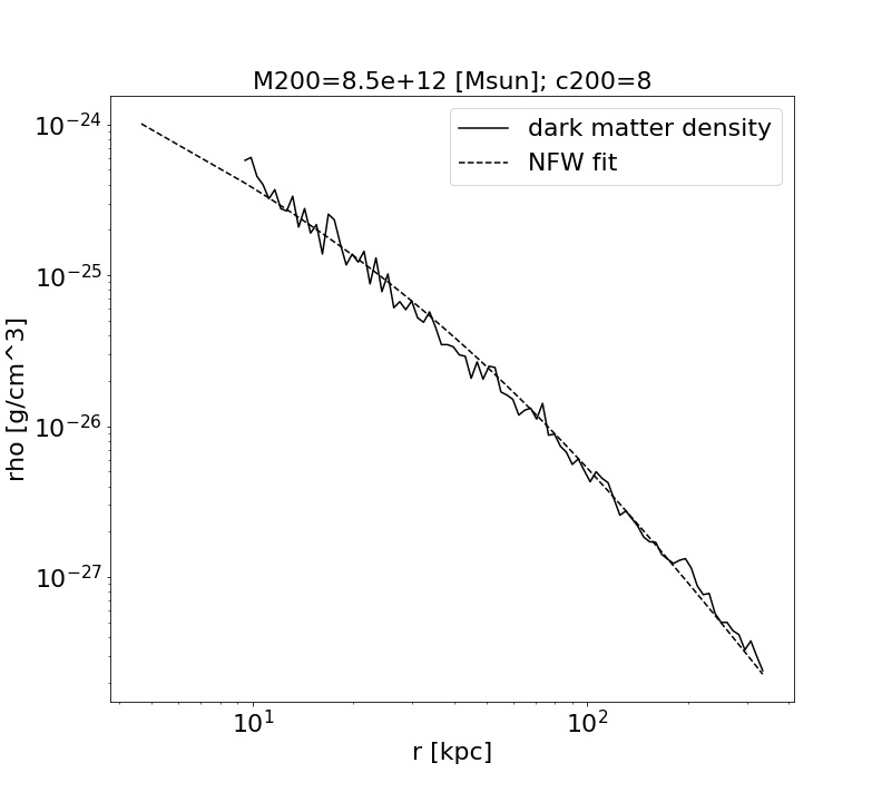
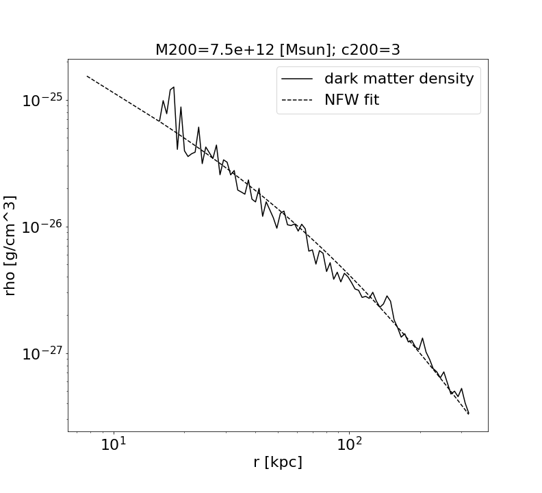
Figure 1: Dark matter density distribution and NFW fit profile of two haloes, one with a high concentration (left panel) and one with a low concentration (right panel)

The scale radius $r_{s}$ is order of magnitudes above the resolution limit of the simulation (for instance, the softening lengths $\epsilon$ and $\epsilon_{\star}$ in Table 1), making it a well resolved value. The NFW fit is performed over $50$ logarithmic bins of the dark matter density, up to $R_{200}.$ The first bin runs from the centre of the halo to the minimum distance that contains $100$ particles. Figure 1 shows the dark matter density profile and the corresponding NFW fit for a low concentrated and a high concentrated halo.

We performed the fit for various redshift bins $z=0,0.5,1,1.5,2$ and over the whole range $z=0-2$. The fit was performed using the average concentration computed in $20$ logarithmic mass bins that span the whole mass range. The pivot mass $10^{13}M_{\odot}$ is the median mass of all selected haloes.

When we extract all haloes in a mass range over different snapshots from a simulation, it happens that most haloes at high redshift will be re-selected at lower redshift. We argue that this does not introduce a bias in the selection: in fact, the time between the two snapshots is longer than the dynamical time of the halo, ensuring that there is no correlation between the dynamical states of the two objects after such a long period of time.

We then fit the concentration as a function of both mass and redshift, with the following functional form:

$$c_{200}=A\cdot\left(\frac{M_{200}}{10^{13}M_{\odot}}\right)^{B}\left(\frac{1.47}{1+z}\right)^{C}.$$ (2)

Table 3: Fit parameters of $c_{200}(M_{200})$ as a power law of the halo mass as in Equation 1 for each redshift bin.

redshift	A	B
$z=0$	$6.25\pm 0.07$	$-0.121\pm 0.004$
$z=0.5$	$5.79\pm 0.07$	$-0.122\pm 0.004$
$z=1$	$5.26\pm 0.08$	$-0.123\pm 0.007$
$z=1.5$	$5.36\pm 0.07$	$-0.117\pm 0.006$
$z=2$	$5.37\pm 0.07$	$-0.097\pm 0.006$
$z=0-2$	$5.74\pm 0.07$	$-0.104\pm 0.004$

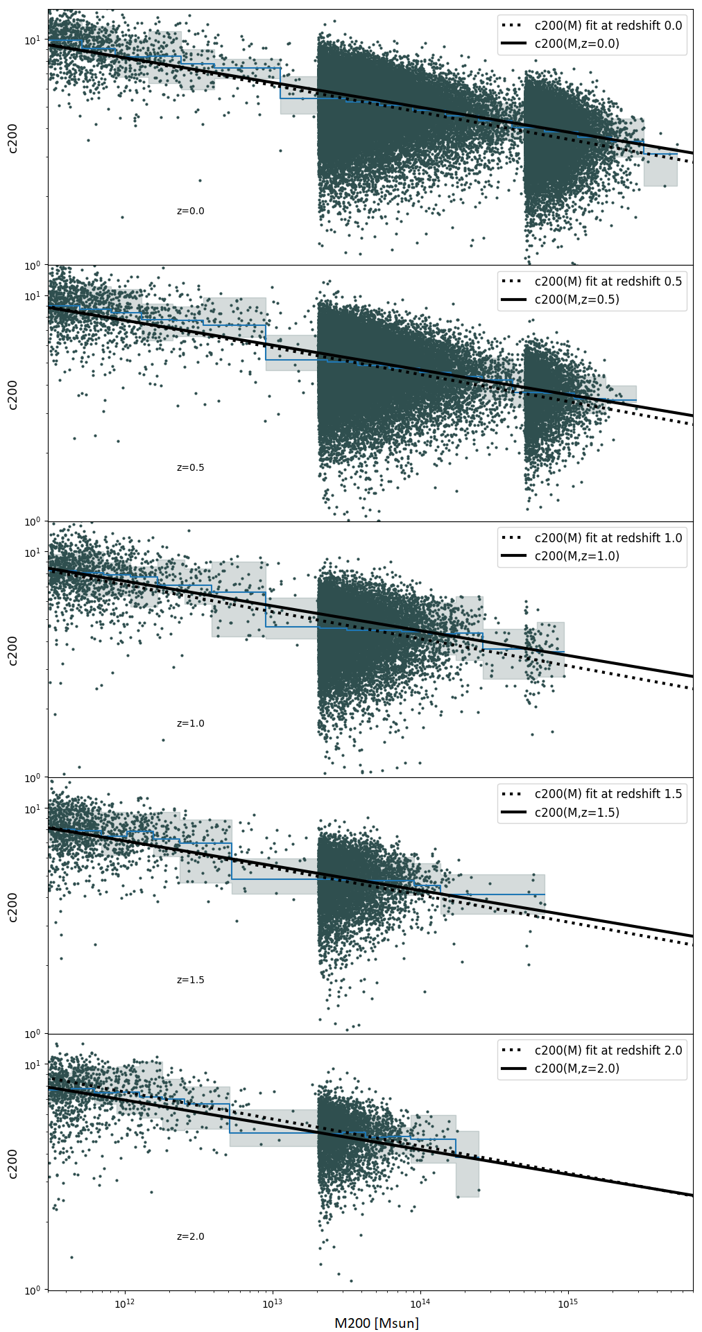
Figure 2: Mass-concentration relation for the well resolved haloes in the three Magneticum simulations Box4/uhr, Box2b/hr and Box0/mr (dark points). Each simulation covers three different mass ranges, respectively $M_{200}>3\cdot 10^{11}M_{\odot},M_{200}>2\cdot 10^{13}M_{\odot}$ and $M_{200}>5\cdot 10^{14}M_{\odot}$ . In each panel we show haloes of a different redshift bin, the median of the concentration(blue curve), the locus containing $50\%$ of points (shaded area), the fit obtained with a $c_{200}(M_{200})$ fit as in Equation 1 and $c_{200}(M_{200},z)$ as in Equation 2 (dotted and solid lines, respectively).

Table 3 shows the fit parameters and their errors that are given by the cross-correlation matrix. The concentration at $10^{14}M_{\odot}$ evolves very weakly with redshift. In order to confirm this, for all selected haloes presented in Table 2, we also performed a fit of the halo concentration as a power law of mass and redshift using the relation

The fit was made on the average concentration of the haloes binned by the $5$ redshift bins on the same mass bins as before and for the redshift dependency we use the median redshift value of $1.47$ as pivot. The fit, performed over all objects gives:

$$\begin{split}A=&6.02\pm 0.04\\ B=&-0.12\pm 0.01\\ C=&0.16\pm 0.01\\ \end{split}$$ (3)

We can see that the redshift dependency, represented by the parameter C, is low although it differs from zero.

Figure 2 shows the mass-concentration plane of Magneticum haloes, where different panels display data at different redshifts. Over-plotted are the fit relations for $c_{200}\propto M_{200}^{B}$ and $c_{200}\propto M_{200}^{B}\cdot(1+z)^{-C}.$

Table 4: Mass ranges and fit parameters of the mass-concentration relation in literature. The value of $c_{200}(10^{14}M_{\odot})$ is extrapolated at $z=0$ when the relative error in the fit parameter is smaller than few percents (when provided). Concentration in Bullock et al. (2001) has been converted from $c_{vir}$ to $c_{200}.$

authors	mass range $[M_{\odot}]$			slope	$c_{200}(10^{14}M_{\odot})$	comments
Bullock et al. (2001)	$10^{11}$	$-$	$10^{14}h^{-1}$	$\approx-0.3$	$4.1$	N-body
Pratt & Arnaud (2005)	$10^{14}$	$-$	$10^{15}$	$N/A$	$4-6$	X-ray from XMM-Newton
Neto et al. (2007)	$10^{12}$	$-$	$10^{15}h^{-1}$	$-0.1$	$4.8$	N-body from Millennium
Mandelbaum et al. (2008)	$10^{12}$	$-$	$10^{15}h^{-1}$	$-0.13\pm 0.07$	$4.8$	weak lensing via SDSS
Bhattacharya et al. (2013)	$\sim 3\cdot 10^{12}$	$-$	$10^{15}h^{-1}$	$-0.08$	$4.7$	N-body
Martinsson et al. (2013)	$10^{11}$	$-$	$10^{12}$	$N/A$	$N/A$	Subset of DiskMass survey
Dutton & Macciò (2014)	$10^{12.5}$	$-$	$10^{14.5}h^{-1}$	$-0.905$	$5.2$	N-body
Meneghetti et al. (2014)	$6\cdot 10^{14}$	$-$	$10^{15}h^{-1}$	$-0.058$	$N/A$	CLASH mock observations
Ludlow et al. (2014)	$10^{12}$	$-$	$10^{15}h^{-1}$	$-0.1$	$5.5$	N-body from Millennium
Covone et al. (2014)	$3\cdot 10^{13}$	$-$	$2\cdot 10^{14}h^{-1}$	$0.09$	$5.4$	lensing from CFHTLenS
Correa et al. (2015)	$N/A$			$-0.08$	$3.8$	semi-analytical model
Merten et al. (2015)	$5\cdot 10^{14}$	$-$	$2\cdot 10^{15}$	$-0.32\pm 0.18$	$N/A$	lensing+X rays on CLASH data
Mantz et al. (2016)	$5\cdot 10^{14}$	$-$	$2\cdot 10^{15}$	$-0.15$	$N/A$	lensing and X-ray from Chandra and ROSAT
Groener et al. (2016)	$\sim 10^{15}$			$-0.16$	$N/A$	comprehensive study on lensing data
Klypin et al. (2016)	$10^{11}$	$-$	$10^{15}h^{-1}$	$-0.12$	$4.1$	N-body from MultiDark
Shan et al. (2017)	$5\cdot 10^{12}$	$-$	$2\cdot 10^{14}$	$-0.13$	$3.3$	weak lensing on SDSS/BOSS
Biviano et al. (2017)	$10^{14}$	$-$	$2\cdot 10^{15}$	$-0.11\pm 0.1$	$4.6$	dynamics of OmegaWINGS clusters
Shirasaki et al. (2018)	$5\cdot 10^{14}$	$-$	$2\cdot 10^{15}$	$-0.14$	$5.6$	Omega$500$ hydrodynamic simulations
This work	$10^{11}$	$-$	$10^{15}$	$-0.1$	$4.5$	Hydro N-body from Magneticum

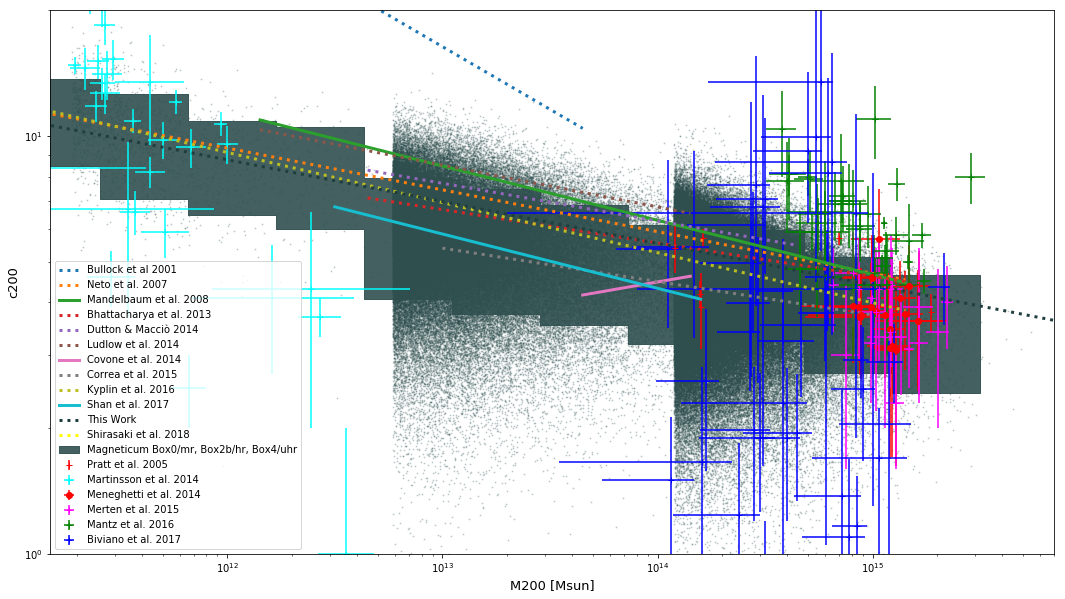
Figure 3: The mass-concentration relation. Dark green points are haloes from the Magneticum simulations (see Table 1) at $z=0$, dark shaded area contains $95\%$ of points within the median. Black dashed line is the $c_{200}(M_{200})$ median for Magneticum data points. Dashed lines are predictions from simulations and solid lines are fit from observed concentrations, both at $z=0$. Error bars are from observations from dynamical mass analyses, with no redshift corrections. All mass conversions are made assuming $h=0.704.$

Table 4 reports a review of the slope values of the mass-concentration plane found on both theoretical and observational works. Figure 3 shows a plot of the same data. When the slope of the mass-concentration relation had an uncertainty smaller than few percents, we extrapolated the value of the concentration at the mass of $10^{14}M_{\odot}$ using $h=0.704.$

Bullock et al. (2001) present one of the first analytical and numerical work on concentration in simulations. They predicted the concentration within the virial radius, that in this work has been converted to a concentration over $R_{200}.$ Although their simulations were performed with a relatively low resolution, their concentration extrapolated at $10^{14}M_{\odot}$ is within the scatter of present days studies. Neto et al. (2007) employ the first very large dark matter-only N-body cosmological simulation, the Millennium simulation, see Springel (2005) where they constrain the mass-concentration dependency accurately over several orders of magnitudes in mass for dark matter only runs.

Pratt & Arnaud (2005) use X-ray data from XMM-Newton, Mandelbaum et al. (2008); Shan et al. (2017) use lensing from SDSS images, while Covone et al. (2014); Mantz et al. (2016); Groener et al. (2016); Covone et al. (2014); Umetsu et al. (2016) combine both lensing and X-ray reconstruction techniques to find the concentration of the dark matter component of haloes. Observations with X-ray data have usually high uncertainties and need to make assumptions on the dependency between the baryon and the dark matter profiles, producing data with large uncertainties. The low mass regime of the plot shows observations of galaxies from the DiskMass survey from Martinsson et al. (2013). Points from the DiskMass survey cover a very large range of concentration values for low massive haloes, in contrast with simulations. Correa et al. (2015) adopted a semi-analytical model (SAM) that predicts concentration over 5 orders of magnitude. Groener et al. (2016) stack all observational mass-concentration data found in literature and made a single fit from it. Klypin et al. (2016) show the results of the MultiDark N-body simulation and produce a lower concentration than Magneticum haloes. Meneghetti et al. (2014) present a numerical work called MUSIC of CLASH where a number of simulated haloes have been chosen to make mock observations for CLASH. Mantz et al. (2016) present results from observations of relaxed haloes. These haloes have a higher concentration in agreement with theoretical studies. The high mass regime of the plot shows results from observations from WINGS (Biviano et al., 2017) and from CLASH (Merten et al., 2015). It must be taken into account that the galaxies from the DiskMass survey are a restricted sub-sample of a very large initial sample. Those galaxies have been chosen so that it is possible to compute the concentration. This may have introduced a significant bias in the concentration estimate. Merten et al. (2015); Biviano et al. (2017); Pratt & Arnaud (2005); Martinsson et al. (2013) compute halo properties using dynamical analyses which have larger uncertainties. The Omega500 simulations (see e.g. Shirasaki et al., 2018) are hydrodynamic simulation that include radiative cooling, star formation and AGN feedback.

Magneticum low-mass haloes have comparatively lower concentration of the dark matter profile than dark matter only simulations.

4 Concentration and fossil parameter

The previous section showed how the concentration can span over an order of magnitude on both observational and theoretical works. In this section we show how the scatter is partially related to “how much” a halo is fossil. We first define a fossilness parameter and then study the evolution over time of both the fossilness and the concentration in some special objects.

Pratt et al. (2016); Kundert et al. (2015); Khosroshahi et al. (2006); Humphrey et al. (2012, 2011); Buote (2017) show how fossil objects have a higher concentration than the average.

More generally, simulations found that dynamically relaxed haloes have a higher concentration (see e.g. Klypin et al., 2016).

A fossil object has been defined by Voevodkin et al. (2010) as having a difference in magnitude in the $R$ band $\Delta m_{R}\geq 1.7$ between the most luminous object and the second most luminous object within a distance of $\frac{1}{2}R_{200}$ from the centre.

In our theoretical work we adapt the definition of the fossil parameter by quantifying it as the stellar mass ratio between central galaxy and most massive satellite:

$$\rm{fossilness}=\frac{M_{\star,\rm{central}}}{\rm{max}\left\{M_{\star,\rm{satellite}}\right\}}.$$ (4)

We also extended the search of all satellites to $R_{200}$ (instead of $\frac{1}{2}R_{200}$ proposed by Voevodkin et al. (2010)) because we consider objects outside $R_{200}$ not to contribute to the dynamical state.

We convert the observed magnitude difference to a fossil parameter by assuming a constant ratio between galaxy masses and luminosities,

$$\rm{fossilness}=10^{\Delta m_{R}/2.5}.$$ (5)

This implies that the $\Delta m_{R}\geq 1.7$ threshold defined in Voevodkin et al. (2010) corresponds to a fossilness of

$$\rm fossilness\gtrsim 4.5.$$ (6)

4.1 Concentration as a function of the fossil parameter

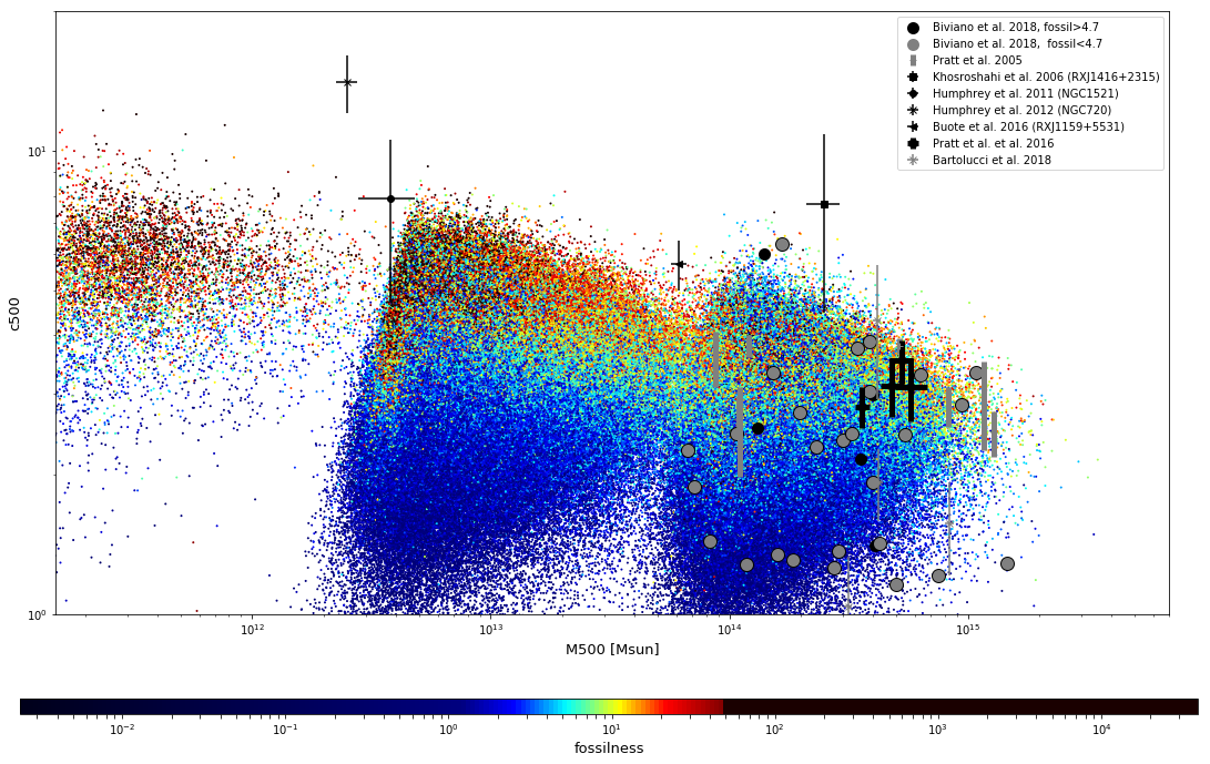
Figure 4: Mass-concentration plane. Mass and radius are computed using $\Delta_{500}$. Points are from the Magneticum data and they are colour coded by fossil parameter (defined as the ratio between stellar masses of the central galaxy and the most massive satellite). The colour saturates to black for the $10\%$ outliers in concentration. Fossil objects from Khosroshahi et al. (2006); Humphrey et al. (2011, 2012); Pratt et al. (2016); Buote (2017) are coloured in black, haloes from Pratt & Arnaud (2005); Bartalucci et al. (2018); Biviano et al. (2017) are coloured in grey. Data from Biviano et al. (2017) is divided between high and low fossilness according to Equation 6.

Figure 4 shows the Magneticum haloes concentration as a function of halo mass, colour coded by fossilness. We also show observational data of fossil groups taken from Khosroshahi et al. (2006); Humphrey et al. (2011, 2012); Pratt et al. (2016); Buote (2017) and haloes from Pratt & Arnaud (2005); Biviano et al. (2017); Bartalucci et al. (2018). Since most observational data were provided in terms of $R_{500}$ and $c_{500},$ in this plot we show mass and concentration computed using $\Delta=500$ for all data points. Haloes from Biviano et al. (2017) are colour coded by fossilness by converting the difference in magnitude to ratio of luminosities.

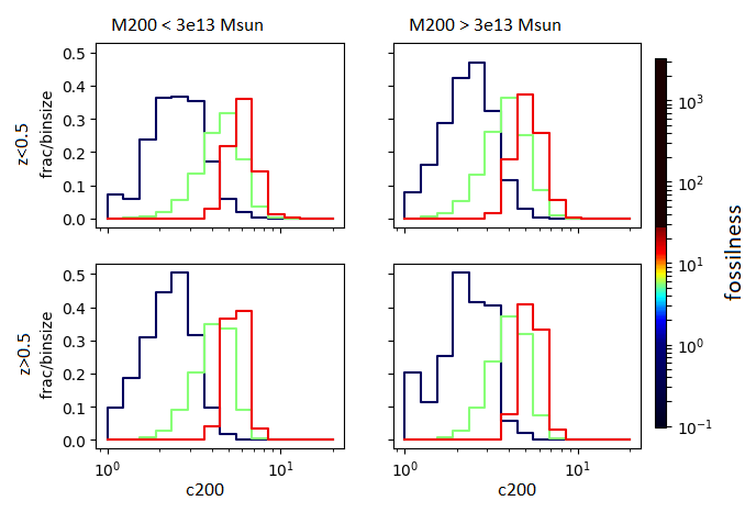
Figure 5: Distribution of concentration for various fossilness values. Left panels contain low mass haloes ($M_{200}<3\cdot 10^{13}M_{\odot}$) and right panels contain high mass haloes ($M_{200}>3\cdot 10^{13}M_{\odot}$) , while top row refers to low redshift haloes ($z\leq 0.5$) and bottom row refers to high redshift haloes ($z>0.5$).

Figure 5 shows the concentration distribution for various mass, redshift and colour coded by fossilness bins. We can see that at each mass and redshift bin, the concentration increases with the fossil parameter, while the spread decreases as the fossil parameter increases.

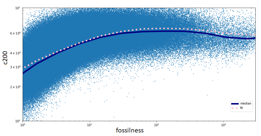
Figure 6: Concentration vs. fossilness for Magneticum data. Over plotted are the median, the concentration depending a double power law of the fossilness.

There is a change in slope for very high value of the fossilness parameter so we modelled the dependence of concentration with slopes (see Figure 6, with also the fit results):

$$\begin{split}c_{200}=&A\cdot\left(\frac{M_{200}}{10^{13}M_{\odot}}\right)^{B}\left(\frac{1.47}{1+z}\right)^{C}\cdot\\ &\cdot\left(\frac{\rm{fossilness}}{F_{0}}\right)^{D}\left(1+\frac{\rm fossilness}{F_{0}}\right)^{E-D}.\end{split}$$ (7)

The fit was performed with the binning technique as for the previous fits. Additionally, the fossil parameter was binned over $20$ logarithmic bins of $fossilness>1.$ In this case, the exponent $E$ maps the asymptotic exponent of $c_{200}$ for high values of fossil parameters, while $D$ is the exponent for low values of the fossil parameter. The value of $F_{0}$ in the fit should should indicate where the two regimes of the fossilness slope starts to change.

Table 5: Fit parameters of $c_{200}(M_{200})$ as a function of mass, redshift and fossil parameter as in Equation 7.

Fit parameter	Value
$A$	$7.5\pm 0.1$
$B$	$-0.1\pm 0.1$
$C$	$0.13\pm 0.01$
$D$	$0.40\pm 0.03$
$E$	$-0.015\pm 0.003$
$F_{0}$	$4.8\pm 0.7$

Table 5 show the fit results. There it is possible to see the positive correlation between concentration and fossilness (parameters $D$ and $D-E$ are positive). Figure 6 shows the fitting relation as well as the data for single haloes and their median. For higher values it is necessary to use a double slope relation.

4.2 Concentration evolution in time

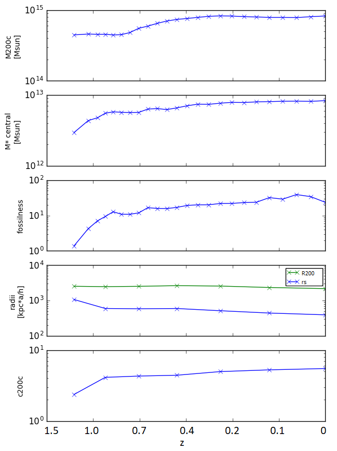
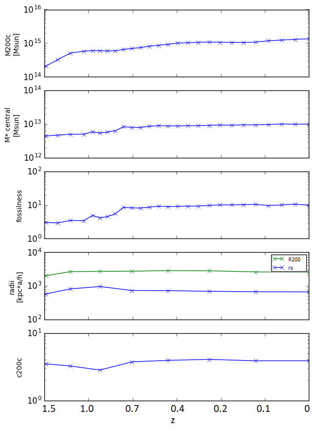
Figure 7: The evolution over time of two haloes (left and right panels) from Box0/mr: $M_{200},$ stellar mass of central galaxy, fossil parameter, $R_{200}$ (in green) and $r_{s}$ in (blue) and concentration from to to bottom. Both objects have been selected because they had an increasing fossil parameter. As long as their central galaxy accretes satellites and keep accreting mass, the scale radius decreases and in turn, decreases the concentration to decrease, thus the relationship between concentration and fossilness.

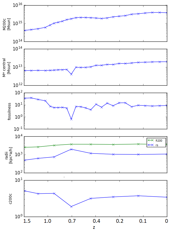
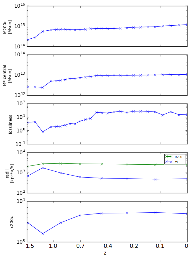
Figure 8: As for Figure 7 but for objects that have a single major merger in their history.

In order to understand what brought fossil objects such a high concentration, we followed the evolution of concentration and fossilness for a number of objects in the simulation Box/0mr. We present here two of the few most massive objects where fossil parameter increased from $z=1.5$ to $z=0$. They have more than $10^{5}$ particles and a final mass $M_{200}\approx 10^{15}M_{\odot}.$ Figure 7 shows the evolution of halo mass, the stellar mass of central galaxy, scale radius, halo radius, fossilness and concentration of these haloes. In these examples it is very easy to see that as long as their central galaxy accretes satellites and keeps accreting mass, the scale radius decreases and makes their concentration higher and higher.

Additionally, in Figure 8 we show the evolution of two haloes that happen to have only one major merger in their history. When a merger happens then the fossil parameter drops because new massive satellites enter the system and the fossilness value decreases (see Eq. 4). As already expected from previous theoretical studies (Neto et al., 2007) we can see that the concentration goes down.

Neto et al. (2007) showed how the scatter in concentration can be partially described by the formation time, in this subsection we showed how a shift in concentration caused by a slow and steady increase of the concentration (led by a decrease of $r_{s}$) brings future fossil groups in the top region of the mass-concentration plane.

5 Virial ratio and concentration

In this section we study how the virial ratio of Magneticum haloes depend on the concentration and fossilness.

The moment of inertia $I$ of a collisionless fluid under a force given by its gravitational potential $\Phi$, obeys the time evolution equation:

$$\frac{1}{2}\frac{d^{2}I}{dt}=2K+W-E_{s},$$

where the kinetic energy $K$ includes the internal energy of gas, $W$ is the total potential energy of the system and $E_{s}$ is the energy from the surface pressure $P$ at the halo boundary:

$$E_{s}=\int_{S}P(\vec{r})r\cdot d\vec{S}.$$

The pressure takes into account the pressure from the gas component.

A system at the equilibrium is supposed to have the so called virial ratio $\eta=1,$ where

$$\eta\equiv-\frac{2K-E_{s}}{W}.$$

For more details on how to compute these quantities and integrals see Chandrasekhar (1961); Binney & Tremaine (2008); Cui et al. (2017).

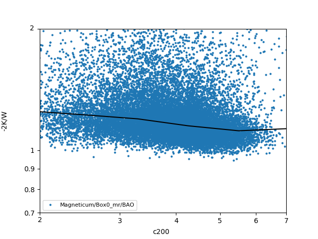
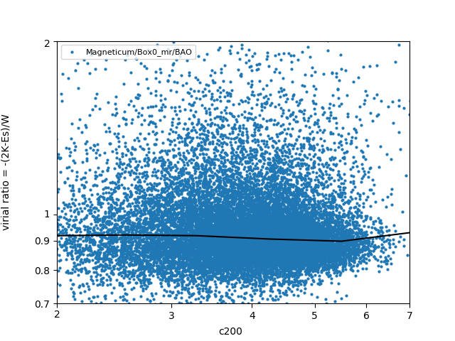
Figure 9: Virial ratio without (left panel) and with (right panel) the correction from the pressure term, as a function of the concentration for the simulation Magneticum/Box0/mr.

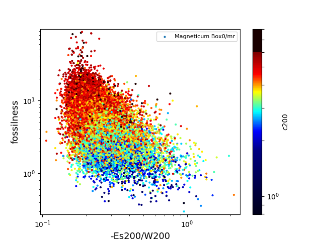
Figure 10: Fossilness versus virial ratio for Magneticum/Box0/bao run, colour coded by concentration (colour bar on the right). The colour saturates to black for the $10\%$ outliers in concentration.

Figure 9 (left panel) shows the ratio $-2K/W$ versus the concentration for the haloes in the Magneticum Box0/mr run while Figure 9 (right panel) shows $\eta$ versus the concentration. The median $\eta$ is close to $0.9$ and it is generally lower than the median of $-2K/W.$ Theoretical works as Klypin et al. (2016) found a lower virial ratio when considering the term $E_{s}.$ From the figures we can see that there is a correlation between concentration and $-2K/W,$ while the correlation is much weaker if we add $E_{s}$ to the kinetic term.

Table 6: Fit parameters of mass-concentration relation for relaxed, un-relaxed and all clusters performed $z=0$ and with a pivot mass of $10^{14}M_{\odot}$

Fit function $c_{200}=A\cdot\left(\frac{M_{200}}{10^{14}M_{\odot}}\right)^{B}$
Halo samples	A	B
relaxed	$5.2\pm 0.1$	$-0.1\pm 0.1$
un-relaxed	$4.3\pm 0.1$	$-0.1\pm 0.1$
complete sample	$4.8\pm 0.1$	$-0.1\pm 0.1$

We identify un-relaxed clusters by selecting haloes with $-2K/W$ lower than $0.5$ or greater than $1.5.$ Those objects have either a large imbalance between the total gravitational energy and the kinetic energy or a large energy from the surface pressure (and thus an inflow/outflow of material). Table 6 shows the fit performed at $z=0$ with the binning technique as for the previous fits of Eq. 1. We used a pivot mass of $10^{14}M_{\odot}$ in order to easily compare it with observations. The values are in agreement with recent observations on SZE selected galaxy clusters (see e.g. Table 7 in Capasso et al., 2019).

Figure 10 shows the fossil parameter as a function of $E_{s}/W$ colour coded by the concentration. Fossil objects have lower $E_{s}$ (accreting less material from outside) than other clusters, thus their more external region has no activity (no in-fall or outfall of material). This is also in agreement with Figure 7 where the evolution of fossil concentration is dominated by their internal motions (central galaxy accretes satellites).

6 Conclusions

We used three cosmological hydrodynamic simulations from the Magneticum suite to cover a mass range from $3\cdot 10^{11}$ to $6\cdot 10^{15}M_{\odot}$ of well resolved clusters from redshift zero to redshift $2$ and we computed the concentration for all well resolved haloes and fit it as a power law of mass and redshift.

This is the first study of the mass-concentration relation in hydrodynamic simulations covering several orders of magnitude in mass. For high massive clusters, we found a value of the concentration and its dependency on mass and redshift is in agreement within the large scatter already present in both observations and simulations.

An exception is made for the low mass regime, wherein the Magneticum simulation concentration (of the dark matter density) is systematically lower than concentration found in studies based on dark matter only simulations. Such different behaviour is in agreement with other theoretical studies where the activation of AGN feedback in low mass haloes is capable of lowering the concentration up to a factor of $\approx 15\%$ (see Figure 8 in Duffy et al., 2010) by removing baryons from the inner region of the halo. These effects have also been reproduced by the NIHAO hydrodynamic cosmological simulations with high spatial resolution that reaches down to $3\cdot 10^{3}M_{\odot}$ per gas particle. Butsky et al. (2016) find a flattening of the core region when comparing the dark matter density profile of a hydrodynamic run against its DMO counter part and an overall decrease in $M_{200}$ (Dutton et al., 2016). In fact, the presence of baryons proved to be able to make dark matter haloes to be less cuspy (Dutton et al., 2018). These effects contribute in lowering the concentration of dark matter density profiles of low-mass haloes (with respect to DMO runs). Thanks to the high mass regime of the Magneticum simulations we are able to capture this effect and its disappearance as the halo mass increases.

In the second part of this work we discussed the origin of the large scatter of concentration in the mass-concentration plane by studying its dependency on the fossilness. Fossil groups are supposed to have had a long period of inactivity and are known to have a higher concentration (see e.g. Neto et al., 2007; Dutton & Macciò, 2014; Pratt et al., 2016). Since we are working with hydrodynamic simulations, we compare halo fossilness (stellar mass ratio between central and most massive satellite of the system, as in see Eq. 4) with observations. We find that the large statistics of Magneticum simulations is able to reproduce these rare objects. Thanks to the large number of objects we are able to fit the concentration as a function of mass, redshift and fossil parameter (see Table 5), where we find a positive correlation between concentration and fossil parameter.

We also investigate the underlying mechanism that brings fossil groups to the highest part of the mass-concentration plane. For this reason we followed the time evolution of some haloes. Here we showed that in unperturbed haloes, both fossilness and concentration steadily and slowly grow with time (see Figure 7). This is in contrast with more naive models where an unperturbed halo keeps its concentration making it a mere function of its collapse time (as in Bullock et al., 2001). Interestingly, we found that this change of concentration is due to a decline of the scale radius. We also showed how the scale radius and fossilness increase or decrease together when a major merger occurs (see Figure 8). From these analyses, we found that those two effects drive the correlation between concentration and fossil parameter. Our findings are not in contrast with the fact that relaxed and fossil objects start with a high concentration because of their early formation times, but we show how an additional steady increase of the concentration pushes these objects in the very high region of the mass-concentration plane.

We then examined the concentration as a function of the virial ratio $\eta=-(2K-E_{s})/W$ and as a function of the energy from the surface pressure. We found a weak dependency of the concentration on $-(2K-E_{s})/W$ and very weak on the terms $-2K/W$ and $E_{s}.$ While a large value of $E_{s}$ means that the cluster has a considerable amount of in-falling material and this translates into a low concentration and low fossil parameter; while a low value of $E_{s}$ (no in-falling material) can be related to both high and low concentrated clusters. The difference between $-2K/W$ and $-\left(2K-E_{s}\right)/W$ is higher for haloes with lower concentration. This implies that low concentration objects are accreting material from the outside and it is in agreement with the idea that low-concentration haloes are not relaxed. This is compatible with other theoretical works as Klypin et al. (2016). This last analyses also showed that (see Figure 10) how fossil objects have both high concentration and a low value of $E_{s},$ indicating a low accretion rate. Our findings point to the direction that fossil objects lived un-perturbed, accreted all massive satellites and have no in-fall/outfall material.

Work has still to be done to study the relation between fossil parameter and other quantities that are well known to be tied with the dynamical state of a system, for instance, the difference between centre of mass and density peak position), or the velocity dispersion deviation between the one inferred from the virial theorem. Additional work is also needed in order to understand the connection between central galaxy accreting satellites and the redistribution of the angular momentum within the halo, which in turn may give hints on the weak dependency between concentration and spin parameter (as found by Macciò et al., 2008).

References

- Bartalucci et al. (2018) Bartalucci I., Arnaud M., Pratt G. W., Le Brun A. M. C., 2018, A&A, 617, A64
- Beck et al. (2016) Beck A. M., et al., 2016, MNRAS, 455, 2110
- Bellstedt et al. (2018) Bellstedt S., et al., 2018, MNRAS, 476, 4543