Burnett Spectral Method for the Spatially Homogeneous Boltzmann Equation

Abstract

We develop a spectral method for the spatially homogeneous Boltzmann equation using Burnett polynomials in the basis functions. Using the sparsity of the coefficients in the expansion of the collision term, the computational cost is reduced by one order of magnitude for general collision kernels and by two orders of magnitude for Maxwell molecules. The proposed method can couple seamlessly with the BGK-type modelling techniques to make future applications affordable. The implementation of the algorithm is discussed in detail, including a numerical scheme to compute all the coefficients accurately, and the design of the data structure to achieve high cache hit ratio. Numerical examples are provided to demonstrate the accuracy and efficiency of our method.

Keywords: Boltzmann equation, Burnett polynomials, collision operator

1 Introduction

The Boltzmann equation possesses its unambiguous significance in the rarefied gas dynamics. Using a velocity distribution function $f\in L^{1}(\mathbb{R}^{3})$ to describe the statistical behavior of gas molecules, the Boltzmann equation incorporates the transport and the collision of particles into a single equation, which accurately models the gas flow from transitional to free molecular regimes. By the molecular chaos assumption, the collision between molecules gives the rate of change for the distribution function as follows:

$$\mathcal{Q}[f,f](\boldsymbol{v})=\int_{\mathbb{R}^{3}}\int_{\boldsymbol{n}\perp\boldsymbol{g}}\int_{0}^{\pi}B(|\boldsymbol{g}|,\chi)[f(\boldsymbol{v}_{1}^{\prime})f(\boldsymbol{v}^{\prime})-f(\boldsymbol{v}_{1})f(\boldsymbol{v})]\,\mathrm{d}\chi\,\mathrm{d}\boldsymbol{n}\,\mathrm{d}\boldsymbol{v}_{1},$$ (1.1)

where $\boldsymbol{n}$ is a unit vector and

$$\boldsymbol{g} =\boldsymbol{v}-\boldsymbol{v}_{1},$$

$$\boldsymbol{v}^{\prime} =\cos^{2}(\chi/2)\boldsymbol{v}+\sin^{2}(\chi/2)\boldsymbol{v}_{1}-|\boldsymbol{g}|\cos(\chi/2)\sin(\chi/2)\boldsymbol{n},$$

$$\boldsymbol{v}_{1}^{\prime} =\cos^{2}(\chi/2)\boldsymbol{v}_{1}+\sin^{2}(\chi/2)\boldsymbol{v}+|\boldsymbol{g}|\cos(\chi/2)\sin(\chi/2)\boldsymbol{n}.$$

The collisional kernel $B(\cdot,\cdot)$ is a nonnegative function involving the differential cross-section of the collision dynamics. Such a high-dimensional integral form introduces great difficulty to the numerical simulation of the Boltzmann equation, and people have been using the stochastic method introduced by Bird [3, 4], known as direct simulation of Monte Carlo (DSMC), to solve the Boltzmann equation. Due to the fast development of super computers, in the past decade, a number of deterministic methods have been proposed to discretize the integral collision term to avoid numerical oscillations. The most promising method seems to be the Fourier spectral method [22, 20, 12], including a variety of its variations such as the conservative version [14], the positivity preserving version [23], the steady-state preserving version [11] and the entropic version [7], where the technique of fast Fourier transform can be applied to accelerate the computation. These methods has been applied to spatially inhomogeneous problems in [29, 28, 10]. Other methods include the fast discrete velocity method [21] and the discontinuous Galerkin method [1].

Another type of spectral method based on global orthogonal polynomials is also being studied recently [8, 13, 25]. In this paper, we follow the work [8, 13] and adopt the spectral method based on Burnett polynomials [6], which has been applied to the linearized Boltzmann equation [8, 9], and shows great potential to achieve higher numerical efficiency. To focus on the collision term, we consider only the spatially homogeneous Boltzmann equation, meaning that the distribution function is uniform in space, and thus we can use a map $F:\mathbb{R}_{+}\rightarrow L^{1}(\mathbb{R}^{3})$ to describe the evolution of the distribution function:

$$\frac{\mathrm{d}F(t)}{\mathrm{d}t}=\mathcal{Q}[F(t),F(t)],\qquad\forall t\in(0,+\infty),$$ (1.2)

$$F(0)=f^{0}\in L^{1}(\mathbb{R}^{3}).$$

It is well-known that the Boltzmann equation preserves the conservation of mass, momentum and energy:

$$\int_{\mathbb{R}^{3}}\begin{pmatrix}1\\ \boldsymbol{v}\\ |\boldsymbol{v}|^{2}\end{pmatrix}\mathcal{Q}[f,f](\boldsymbol{v})\,\mathrm{d}\boldsymbol{v}=0,\qquad\forall f\in L^{1}(\mathbb{R}^{3}).$$ (1.3)

Thus we can choose appropriate nondimensionalization such that the initial value $f^{0}$ in (1.2) belongs to the following set:

$$\mathcal{S}=\left\{f\in L^{1}(\mathbb{R}^{3}):\int_{\mathbb{R}^{3}}\begin{pmatrix}1\\ \boldsymbol{v}\\ |\boldsymbol{v}|^{2}\end{pmatrix}f(\boldsymbol{v})\,\mathrm{d}\boldsymbol{v}=\begin{pmatrix}1\\ 0\\ 3\end{pmatrix}\right\},$$

and by (1.3), for all $t>0$, we always have $F(t)\in\mathcal{S}$. According to Boltzmann’s H-theorem, the steady-state solution of (1.2) is the Maxwellian

$$\mathcal{M}(\boldsymbol{v})=\frac{1}{(\sqrt{2\pi})^{3}}\exp\left(-\frac{|\boldsymbol{v}|^{2}}{2}\right).$$ (1.4)

The Burnett polynomials, which will be used in our discretization, are orthogonal polynomials associated with the weight function $\mathcal{M}(\boldsymbol{v})$. Therefore our numerical method can represent this steady-state solution exactly.

In [25, 17], a similar method using Hermite polynomials, which are also orthogonal polynomials associated with the weight function $\mathcal{M}(\boldsymbol{v})$, is studied. In principle, the spectral methods using Burnett and Hermite polynomials are essentially equivalent, especially when the series is truncated up to the same degree. The Hermite spectral method was introduced long ago by Grad [15] as the moment method. As mentioned in [16, pp. 283], the Hermite spectral method is frequently advantageous due to “the symmetries inherent in the invariant Cartesian tensor”. Such an advantage has been utilized in [25], where the explicit expressions of all the coefficients in the discretization are formulated using these symmetries. However, the superiority of the Burnett polynomials introduced in [6] is the fact that they are eigenfunctions of the linearized collision integral for Maxwell molecules [26]. Even for non-Maxwell molecules, as will be shown in this paper, the coefficients also possess some sparsity due to the rotational invariance of the collision operator. This will result in a considerably faster algorithm in the computation, which makes the spectral method with Burnett polynomials preferable in the simulation.

The same basis functions have been used in [13], where the authors employed numerical integration to find all the coefficients involved in the discretization of (1.2), but the sparsity in the coefficients was not utilized in the computation. In this paper, we are going to focus on the detailed implementation of the algorithm, including a much more accurate way to compute the coefficients, a detailed analysis of the computational cost, and the design of the data structure to achieve high computational efficiency. Meanwhile, we also emphasize the modelling technique introduced in [25] which allows flexible balancing between computational cost and modelling error.

The rest of this paper is organized as follows. In Section 2, we present the framework of the Burnett spectral method to solve the homogeneous Boltzmann equation. In Section 3, the detailed implementation of the algorithm is introduced. We first give an efficient method to compute the coefficients in the Burnett spectral expansion, and then discuss the design of the data structure and the implementation of the algorithm in detail. Some numerical experiments verifying the efficiency of the Burnett spectral method are carried out in Section 4. In Section 5, we list the proof of the theorems in Section 2. Some concluding remarks are made in Section 6.

2 Framework of the Burnett spectral method

Burnett polynomials are introduced in [6] to study high-order approximation to the distribution function for a slightly non-uniform gas. Here we adopt a normalized form and write Burnett polynomials as

$$p_{lmn}(\boldsymbol{v})=\sqrt{\frac{2^{1-l}\pi^{3/2}n!}{\Gamma(n+l+3/2)}}L_{n}^{(l+1/2)}\left(\frac{|\boldsymbol{v}|^{2}}{2}\right)|\boldsymbol{v}|^{l}Y_{l}^{m}\left(\frac{\boldsymbol{v}}{|\boldsymbol{v}|}\right),\qquad l,n\in\mathbb{N},\quad m=-l,\cdots,l,$$

where we have used Laguerre polynomials

$$L_{n}^{(\alpha)}(x)=\frac{x^{-\alpha}\exp(x)}{n!}\frac{\mathrm{d}^{n}}{\mathrm{d}x^{n}}\left[x^{n+\alpha}\exp(-x)\right],$$

and spherical harmonics

$$Y_{l}^{m}(\boldsymbol{n})=\sqrt{\frac{2l+1}{4\pi}\frac{(l-m)!}{(l+m)!}}P_{l}^{m}(\cos\theta)\exp(\mathrm{i}m\phi),\qquad\boldsymbol{n}=(\sin\theta\cos\phi,\sin\theta\sin\phi,\cos\theta)^{T}$$

with $P_{l}^{m}$ being the associate Legendre polynomial:

$$P_{l}^{m}(x)=\frac{(-1)^{m}}{2^{l}l!}(1-x^{2})^{m/2}\frac{\mathrm{d}^{l+m}}{\mathrm{d}x^{l+m}}\left[(x^{2}-1)^{l}\right].$$

By the orthogonality of Laguerre polynomials and spherical harmonics, one can find that

$$\int_{\mathbb{R}^{3}}\overline{p_{l_{1}m_{1}n_{1}}(\boldsymbol{v})}p_{l_{2}m_{2}n_{2}}(\boldsymbol{v})\mathcal{M}(\boldsymbol{v})\,\mathrm{d}\boldsymbol{v}=\delta_{l_{1}l_{2}}\delta_{m_{1}m_{2}}\delta_{n_{1}n_{2}}.$$

Now we introduce the basis function $\varphi_{lmn}(\boldsymbol{v})$ as

$$\varphi_{lmn}(\boldsymbol{v})=p_{lmn}(\boldsymbol{v})\mathcal{M}(\boldsymbol{v}).$$ (2.1)

For a given distribution function $f\in\mathcal{S}$, we assume that it has the expansion

$$f(\boldsymbol{v})=\sum_{lmn}\tilde{f}_{lmn}\varphi_{lmn}(\boldsymbol{v}),$$ (2.2)

where the sum is interpreted as

$$\sum_{lmn}=\sum_{l=0}^{+\infty}\sum_{m=-l}^{l}\sum_{n=0}^{+\infty}.$$

Suppose the corresponding collision term $\mathcal{Q}[f,f]$ also has the expansion

$$\mathcal{Q}[f,f](\boldsymbol{v})=\sum_{lmn}\tilde{Q}_{lmn}\varphi_{lmn}(\boldsymbol{v}).$$

By the orthogonality of the Burnett polynomials and the bilinearity of the operator $\mathcal{Q}[\cdot,\cdot]$, one can find that

$$\tilde{Q}_{lmn}=\sum_{l_{1}m_{1}n_{1}}\sum_{l_{2}m_{2}n_{2}}A_{lmn}^{l_{1}m_{1}n_{2},l_{2}m_{2}n_{2}}\tilde{f}_{l_{1}m_{1}n_{1}}\tilde{f}_{l_{2}m_{2}n_{2}},$$

where

$$A_{lmn}^{l_{1}m_{1}n_{2},l_{2}m_{2}n_{2}}=\int_{\mathbb{R}^{3}}\overline{p_{lmn}(\boldsymbol{v})}\mathcal{Q}[\varphi_{l_{1}m_{1}n_{1}},\varphi_{l_{2}m_{2}n_{2}}](\boldsymbol{v})\,\mathrm{d}\boldsymbol{v}.$$ (2.3)

Based on this expansion, it is obvious that (1.2) is equivalent to the following ODE system:

$$\frac{\mathrm{d}\tilde{F}_{lmn}(t)}{\mathrm{d}t}=\sum_{l_{1}m_{1}n_{1}}\sum_{l_{2}m_{2}n_{2}}A_{lmn}^{l_{1}m_{1}n_{2},l_{2}m_{2}n_{2}}\tilde{F}_{l_{1}m_{1}n_{1}}(t)\tilde{F}_{l_{2}m_{2}n_{2}}(t),$$ (2.4)

$$\tilde{F}_{lmn}(0)=\tilde{f}_{lmn}^{0}:=\int_{\mathbb{R}^{3}}\overline{p_{lmn}(\boldsymbol{v})}f^{0}(\boldsymbol{v})\,\mathrm{d}\boldsymbol{v},$$

where $\tilde{F}_{lmn}(t)$ are the coefficients in the Burnett series expansion of $F(t)$.

To develop the spectral method, one needs to truncate the Burnett series to restrict the computation to a finite number of coefficients. A common choice is to choose a positive integer $M$ and require that the degree of the polynomial, $l+2n$, to be less than or equal to $M$. Thus the spectral method for the homogeneous Boltzmann equation (1.2) is

$$\frac{\mathrm{d}\tilde{F}_{lmn}(t)}{\mathrm{d}t}=\sum_{\begin{subarray}{c}l_{1}m_{1}n_{1}\\[2.0pt] l_{1}+2n_{1}\leqslant M\end{subarray}}\sum_{\begin{subarray}{c}l_{2}m_{2}n_{2}\\[2.0pt] l_{2}+2n_{2}\leqslant M\end{subarray}}A_{lmn}^{l_{1}m_{1}n_{2},l_{2}m_{2}n_{2}}\tilde{F}_{l_{1}m_{1}n_{1}}(t)\tilde{F}_{l_{2}m_{2}n_{2}}(t),$$ (2.5a)

$$\tilde{F}_{lmn}(0)=\tilde{f}_{lmn}^{0},\qquad l+2n\leqslant M.$$ (2.5b)

These ordinary differential equations can be solved by Runge-Kutta methods. Naively, the computational cost appears to be $O(N^{3})=O(M^{9})$, where $N=(M+1)(M+2)(M+3)/6$ is the total number of $\tilde{F}_{lmn}$, $l+2n\leq M$. It is worth pointing out that there is a prefactor $1/6^{3}$ of $O(M^{9})$ when we count the number of coefficients $A_{lmn}^{l_{1}m_{1}n_{2},l_{2}m_{2}n_{2}}$, and this prefactor will be directly brought into the computational cost of the collision term.

However, the actual computational cost can be reduced to $O(M^{8})$ due to the following sparsity of the coefficients $A_{lmn}^{l_{1}m_{1}n_{2},l_{2}m_{2}n_{2}}$:

Theorem 1.

The coefficient $A_{lmn}^{l_{1}m_{1}n_{2},l_{2}m_{2}n_{2}}$ is zero if $m\neq m_{1}+m_{2}$.

By taking into account such sparsity, we can find that the number of nonzero coefficients $A_{lmn}^{l_{1}m_{1}n_{2},l_{2}m_{2}n_{2}}$ is $O(M^{8})$ with a prefactor $1/297$. This indicates that the evaluation of the collision can be efficient for not too large $M$. Interestingly, for some special collision kernel $B(\cdot,\cdot)$, the computational cost can be further reduced due to the following extra sparsity of the coefficients $A_{lmn}^{l_{1}m_{1}n_{2},l_{2}m_{2}n_{2}}$:

Theorem 2.

If the kernel $B(g,\chi)=\sigma(\chi)$ is independent of $g$, the coefficient $A_{lmn}^{l_{1}m_{1}n_{2},l_{2}m_{2}n_{2}}$ is zero if $l_{1}+2n_{1}+l_{2}+2n_{2}\neq l+2n$.

A well-known type of collision kernel satisfying the above condition is the Maxwell molecules, for which the force between a pair of molecules is always repulsive and proportional to the fifth power of their distance. The sparsity stated in the above theorem allows us to reduce the number of nonzero coefficients to $O(M^{7})$. By a numerical test, we find that the prefactor of $O(M^{7})$ is around $1/(2.2\times 10^{3})$. Moreover, the following result also helps save computational resources:

Theorem 3.

All coefficients $A_{lmn}^{l_{1}m_{1}n_{1},l_{2}m_{2}n_{2}}$ are real.

The proof of all the above theorems will be provided in Section 5. They help us save both memory and computational time. For general collision kernel, by Theorem 1, we do not need to store the zero coefficients, and the constraint $m=m_{1}+m_{2}$ reduces the order of time complexity by $1$. For Maxwell molecules, Theorem 1 and Theorem 2 reduce the order of time complexity by $2$. Theorem 3 does not reduce the order, but by realizing that all the coefficients are real, one can reduce the storage requirement by a half, and the algorithm can also be made faster by avoiding some operations between complex numbers. Actually, we can further reduce the computational cost by using the fact that the distribution functions are real: since

$$\varphi_{lmn}(\boldsymbol{v})=(-1)^{m}\overline{\varphi_{lmn}(\boldsymbol{v})},$$

the coefficients in (2.2) must satisfy $\tilde{f}_{lmn}=(-1)^{m}\overline{\tilde{f}_{l,-m,n}}$ to ensure that $f(\boldsymbol{v})$ is real; therefore, when solving the ordinary differential equations (2.5), we only need to take into account the case $m\geqslant 0$, which cuts down the computational cost by a half. The small prefactor of the computational complexity also indicates the low computational cost is acceptable if $M$ is not too large.

However, the time complexity $O(M^{8})$ (or $O(M^{7})$ for Maxwell molecules) still gives huge computational cost when $M$ is large, especially when solving spatially inhomogeneous problems. To make the computation even cheaper, we adopt the idea in [8, 25] which replaces the right-hand side of (2.5a) by $\tilde{Q}_{lmn}^{*}(t)$, defined as

$$\tilde{Q}_{lmn}^{*}(t)=\left\{\begin{array}[]{ll}\displaystyle\sum\limits_{\begin{subarray}{c}l_{1}m_{1}n_{1}\\[2.0pt] l_{1}+2n_{1}\leqslant M_{0}\end{subarray}}\sum\limits_{\begin{subarray}{c}l_{2}m_{2}n_{2}\\[2.0pt] l_{2}+2n_{2}\leqslant M_{0}\end{subarray}}A_{lmn}^{l_{1}m_{1}n_{2},l_{2}m_{2}n_{2}}\tilde{F}_{l_{1}m_{1}n_{1}}(t)\tilde{F}_{l_{2}m_{2}n_{2}}(t),&\text{if }l+2n\leqslant M_{0},\\[28.0pt] -\mu_{M_{0}}\tilde{F}_{lmn}(t),&\text{otherwise}.\end{array}\right.$$ (2.6)

In practice, one can set $M_{0}$ to be much less than $M$. Thus the quadratic form is only applied to the first few coefficients whose associate polynomials have degree less than or equal to $M_{0}$. When $l+2n>M_{0}$, similar to the BGK-type models, we let the coefficient decay to zero exponentially at a constant rate $\mu_{M_{0}}$. Thereby we get the new model

$$\frac{\mathrm{d}\tilde{F}_{lmn}(t)}{\mathrm{d}t}=\tilde{Q}_{lmn}^{*}(t).$$ (2.7)

As in [25, 8], we choose the decay rate $\mu_{M_{0}}$ to be the spectral radius of the linearized collision operator $\mathcal{L}_{M_{0}}:\mathcal{S}_{M_{0}}\rightarrow\mathcal{S}_{M_{0}}$ defined as

$$\mathcal{L}_{M_{0}}[f](\boldsymbol{v})=\sum_{\begin{subarray}{c}l_{1}m_{1}n_{1}\\[2.0pt] l_{1}+2n_{1}\leqslant M_{0}\end{subarray}}\sum_{\begin{subarray}{c}n_{2}\leqslant(M_{0}-l_{1})/2\end{subarray}}\left(A_{l0n_{1}}^{l0n_{2},000}+A_{l0n_{1}}^{000,l0n_{2}}\right)\tilde{f}_{l_{1}m_{1}n_{2}}\psi_{l_{1}m_{1}n_{1}}(\boldsymbol{v}),$$ (2.8)

where $\mathcal{S}_{M_{0}}=\text{span}\{\psi_{lmn}(\boldsymbol{v}):l+2n\leqslant M_{0}\}\cap\mathcal{S}$. We refer the readers to [8] for more details.

By now, we have obtained the ordinary differential equations to approximate the homogeneous Boltzmann equation (1.2) under the framework of Burnett polynomials. In order to complete this algorithm, we still need to find the values of the coefficients $A_{lmn}^{l_{1}m_{1}n_{1},l_{2}m_{2}n_{2}}$, which will be detailed in the following section. Moreover, the implementation of the algorithm will be discussed deeply to obtain optimal efficiency.

3 Implementation of the algorithm

To implement the algorithm, we first need to find the values of the coefficients $A_{lmn}^{l_{1}m_{1}n_{1},l_{2}m_{2}n_{2}}$. A formula of these coefficients has been given in [19], which reads

$$A_{lmn}^{l_{1}m_{1}n_{1},l_{2}m_{2}n_{2}}=\sum_{l_{3}m_{3}n_{3}}\sum_{l_{4}m_{4}n_{4}}\sum_{n_{4}^{\prime}}\overline{\left(\begin{array}[]{c|c}n_{3}l_{3}m_{3}&nlm\\ n_{4}^{\prime}l_{4}m_{4}&000\end{array}\right)}\left(\begin{array}[]{c|c}n_{3}l_{3}m_{3}&n_{1}l_{1}m_{1}\\ n_{4}l_{4}m_{4}&n_{2}l_{2}m_{2}\end{array}\right)V_{n_{4}n_{4}^{\prime}}^{l},$$ (3.1)

where

$$\begin{split}V_{nn^{\prime}}^{l}&=\frac{1}{8\sqrt{2}\pi^{5/2}}\sqrt{\frac{n!n^{\prime}!}{\Gamma(n+l+3/2)\Gamma(n^{\prime}+l+3/2)}}\int_{0}^{+\infty}\int_{0}^{\pi}B(g,\chi)\left(\frac{g^{2}}{4}\right)^{l+1}\times{}\\ &\qquad L_{n}^{(l+1/2)}\left(\frac{g^{2}}{4}\right)L_{n^{\prime}}^{(l+1/2)}\left(\frac{g^{2}}{4}\right)[(2l+1)^{2}P_{l}(\cos\chi)-1]\exp\left(-\frac{g^{2}}{4}\right)\,\mathrm{d}\chi\,\mathrm{d}g,\end{split}$$ (3.2)

and the notation $(\cdot\mid\cdot)$ denotes Talmi coefficients for equal mass molecules [24]. Due to the sparsity of the Talmi coefficients, the computational cost for evaluating all $A_{lmn}^{l_{1}m_{1}n_{1},l_{2}m_{2}n_{2}}$ required in (2.5) is $O(M_{0}^{14})$. Thus, computing the Talmi coefficients is not an easy task. The reference [2] provides a possible implementation, but the formula involves Wigner 3-$j$ and 9-$j$ symbols, which are also difficult to obtain. Below we are going to propose another method to compute these coefficients $A_{lmn}^{l_{1}m_{1}n_{1},l_{2}m_{2}n_{2}}$ based on the work [25]. The method also has computational cost $O(M_{0}^{14})$, but is much easier to implement.

3.1 Computation of coefficients $A_{lmn}^{l_{1}m_{1}n_{1},l_{2}m_{2}n_{2}}$

In [25], we have calculated the expansion coefficients of the quadratic collision term $\mathcal{Q}[f,f](\boldsymbol{v})$ under the framework of Hermite spectral method. Since both Hermite polynomials and Burnett polynomials are orthogonal polynomials associated with the same weight function, we can express the Burnett polynomials by linear combinations of the Hermite polynomials, and then the coefficients $A_{lmn}^{l_{1}m_{1}n_{1},l_{2}m_{2}n_{2}}$ naturally become a linear combination of the corresponding coefficients in the Hermite spectral method. Since the expressions for the coefficients in the Hermite spectral method have been worked out explicitly in [25], we do not need to bother using the complicated symbols in the quantum theory to find the values of $A_{lmn}^{l_{1}m_{1}n_{1},l_{2}m_{2}n_{2}}$.

Mathematically, the above framework can be formulated as below. In [25], Hermite polynomial $H^{k_{1}k_{2}k_{3}}(\boldsymbol{v})$ is defined as

$$H^{k_{1}k_{2}k_{3}}(\boldsymbol{v})=\frac{(-1)^{n}}{\mathcal{M}(\boldsymbol{v})}\frac{\partial^{k_{1}+k_{2}+k_{3}}}{\partial v_{1}^{k_{1}}\partial v_{2}^{k_{2}}\partial v_{3}^{k_{2}}}\mathcal{M}(\boldsymbol{v}),\quad\forall k_{1},k_{2},k_{3}\in\mathbb{N},$$ (3.3)

where $\mathcal{M}(\boldsymbol{v})$ is given in (1.4). We would like to express the Burnett polynomials as

$$p_{lmn}(\boldsymbol{v})=\sum_{(k_{1},k_{2},k_{3})\in I_{l+2n}}\frac{1}{k_{1}!k_{2}!k_{3}!}C_{lmn}^{k_{1}k_{2}k_{3}}H^{k_{1}k_{2}k_{3}}(\boldsymbol{v}),$$ (3.4)

where $I_{l+2n}$ is the index set

$$I_{l+2n}=\{(k_{1},k_{2},k_{3})\in\mathbb{N}^{3}\mid k_{1}+k_{2}+k_{3}=l+2n\},$$ (3.5)

and the coefficients $C_{lmn}^{k_{1}k_{2}k_{3}}$ can be calculated as

$$C_{lmn}^{k_{1}k_{2}k_{3}}=\int_{\mathbb{R}^{3}}p_{lmn}(\boldsymbol{v})H^{k_{1}k_{2}k_{3}}(\boldsymbol{v})\mathcal{M}(\boldsymbol{v})\,\mathrm{d}\boldsymbol{v}$$ (3.6)

based on the orthogonality of Hermite polynomials

$$\int_{\mathbb{R}^{3}}H^{k_{1}k_{2}k_{3}}(\boldsymbol{v})H^{l_{1}l_{2}l_{3}}(\boldsymbol{v})\mathcal{M}(\boldsymbol{v})\,\mathrm{d}\boldsymbol{v}=\delta_{k_{1}l_{1}}\delta_{k_{2}l_{2}}\delta_{k_{3}l_{3}}k_{1}!k_{2}!k_{3}!.$$ (3.7)

Note that when $l+2n\neq k_{1}+k_{2}+k_{3}$, i.e. the degrees of $H^{k_{1}k_{2}k_{3}}$ and $p_{lmn}$ are not equal, the coefficient $C_{lmn}^{k_{1}k_{2}k_{3}}$ defined by (3.6) is zero due to the orthogonality of both polynomials. Once $C_{lmn}^{k_{1}k_{2}k_{3}}$ is obtained, we just need to substitute (3.4) to the definition of $A_{lmn}^{l_{1}m_{1}n_{1},l_{2}m_{2}n_{2}}$ (2.3), which results in the following formula for these coefficients:

$$A_{lmn}^{l_{1}m_{1}n_{1},l_{2}m_{2}n_{2}} =\sum_{k\in I_{l+2n}}\sum_{i\in I_{l_{1}+2n_{1}}}\sum_{j\in I_{l_{2}+2n_{2}}}\overline{C_{lmn}^{k_{1}k_{2}k_{3}}}C_{l_{1}m_{1}n_{1}}^{i_{1}i_{2}i_{3}}C_{l_{2}m_{2}n_{2}}^{j_{1}j_{2}j_{3}}\times{}$$ (3.8)

$$\qquad\frac{1}{i_{1}!i_{2}!i_{3}!j_{1}!j_{2}!j_{3}!k_{1}!k_{2}!k_{3}!}\int_{\mathbb{R}^{3}}H^{k_{1}k_{2}k_{3}}(\boldsymbol{v})\mathcal{Q}\left[H^{i_{1}i_{2}i_{3}}\mathcal{M},H^{j_{1}j_{2}j_{3}}\mathcal{M}\right](\boldsymbol{v})\,\mathrm{d}\boldsymbol{v}.$$

The second line of (3.8) has already been evaluated in [25, Theorem 1 & 2] (denoted as $A_{k_{1}k_{2}k_{3}}^{i_{1}i_{2}i_{3},j_{1}j_{2}j_{3}}$ therein). Thus we will focus only on the computation of the coefficients $C_{lmn}^{k_{1}k_{2}k_{3}}$ below.

Define

$$S_{-1}=\frac{1}{2}(v_{1}-\mathrm{i}v_{2}),\quad S_{0}=v_{3},\quad S_{1}=-\frac{1}{2}(v_{1}+\mathrm{i}v_{2}),$$ (3.9)

and

$$\gamma_{lm}^{\mu}=\sqrt{\frac{[l+(2\delta_{1,\mu}-1)m+\delta_{1,\mu}][l-(2\delta_{-1,\mu}-1)m+\delta_{-1,\mu}]}{(2l-1)(2l+1)}},$$ (3.10)

the recursive formula of the basis functions [9] is

$$S_{\mu}\psi_{lmn}(\boldsymbol{v}) =\frac{1}{2^{|\mu|}}\left[\sqrt{2(n+l)+3}\gamma_{l+1,m}^{\mu}\psi_{l+1,m+\mu,n}(\boldsymbol{v})-\sqrt{2n}\gamma_{l+1,m}^{\mu}\psi_{l+1,m+\mu,n-1}(\boldsymbol{v})\right.$$ (3.11)

$$\left.+(-1)^{\mu}\sqrt{2(n+l)+1}\gamma_{-l,m}^{\mu}\psi_{l-1,m+\mu,n}(\boldsymbol{v})-(-1)^{\mu}\sqrt{2(n+1)}\gamma_{-l,m}^{\mu}\psi_{l-1,m+\mu,n+1}(\boldsymbol{v})\right],$$

where we set $\psi_{lmn}(\boldsymbol{v})=0$ if $|m|>l$ or either of $l,n$ is negative. Equations of $C_{lmn}^{k_{1}k_{2}k_{3}}$ can be obtained by multiplying (3.11) with $H^{k_{1}k_{2}k_{3}}(\boldsymbol{v})$ and taking integration with respect to $\boldsymbol{v}$ on both sides. The integral of the right-hand side can be written straightforwardly as expressions of $C_{lmn}^{k_{1}k_{2}k_{3}}$, while for the left-hand side, we need to use the recursion formula of Hermite polynomials

$$v_{s}H^{k_{1}k_{2}k_{3}}(\boldsymbol{v})=H^{k_{1}+\delta_{1s},k_{2}+\delta_{2s},k_{3}+\delta_{3s}}(\boldsymbol{v})+k_{s}H^{k_{1}-\delta_{1s},k_{2}-\delta_{2s},k_{3}-\delta_{3s}}(\boldsymbol{v}),\quad s=1,2,3.$$ (3.12)

Since both the Hermite and Burnett polynomials are orthogonal polynomials, integrals including the product of polynomials of different degrees all vanish. Therefore when applying the above operations, we choose $k_{1},k_{2},k_{3}$ such that $k_{1}+k_{2}+k_{3}=l+2n+1$, and the resulting equations for $\mu=-1,0,1$ are respectively

$$a_{l,m+1,n}^{(-1)}C_{l+1,m,n}^{k_{1}k_{2}k_{3}}+b_{l,m+1,n}^{(-1)}C_{l-1,m,n+1}^{k_{1}k_{2}k_{3}} =\frac{1}{2}k_{1}C_{l,m+1,n}^{k_{1}-1,k_{2},k_{3}}-\frac{\mathrm{i}}{2}k_{2}C_{l,m+1,n}^{k_{1},k_{2}-1,k_{3}},$$ (3.13)

$$a_{l,m,n}^{(0)}C_{l+1,m,n}^{k_{1}k_{2}k_{3}}+b_{l,m,n}^{(0)}C_{l-1,m,n+1}^{k_{1}k_{2}k_{3}} =k_{3}C_{l,m,n}^{k_{1},k_{2},k_{3}-1},$$

$$a_{l,m-1,n}^{(1)}C_{l+1,m,n}^{k_{1}k_{2}k_{3}}+b_{l,m-1,n}^{(1)}C_{l-1,m,n+1}^{k_{1}k_{2}k_{3}} =-\frac{1}{2}k_{1}C_{l,m-1,n}^{k_{1}-1,k_{2},k_{3}}-\frac{\mathrm{i}}{2}k_{2}C_{l,m-1,n}^{k_{1},k_{2}-1,k_{3}},$$

where

$$a_{lmn}^{(\mu)}=\frac{1}{2^{|\mu|}}\sqrt{(2(n+l)+3)}\gamma_{l+1,n}^{\mu},\quad b_{lmn}^{(\mu)}=\frac{(-1)^{\mu+1}}{2^{|\mu|}}\sqrt{2(n+1)}\gamma_{-l,n}^{\mu},\quad\mu=-1,0,1,$$ (3.14)

and we have exchanged the left-hand side and the right-hand side since we would like to solve the coefficients $C_{l+1,m,n}^{k_{1}k_{2}k_{3}}$ and $C_{l-1,m,n+1}^{k_{1}k_{2}k_{3}}$ from the above equations. This is possible since on the left-hand sides of (3.14), the sum of the superscripts $k_{1}+k_{2}+k_{3}$ is always greater than the same sum on the right-hand sides. Hence we can solve all the coefficients $C_{lmn}^{k_{1}k_{2}k_{3}}$ by the order of $k_{1}+k_{2}+k_{3}$, so that the right-hand sides of (3.13) are always known. To start the computation, we need the “initial condition” $C_{000}^{000}=1$, and the “boundary conditions” $C_{lmn}^{k_{1}k_{2}k_{3}}=0$ if $|m|>l$ or either of $l,n$ is negative. It is not difficult to see that the computational cost for each coefficient is $O(1)$, and thus the time complexity for computing all the coefficients $C_{lmn}^{k_{1}k_{2}k_{3}}$ with $l+2n=k_{1}+k_{2}+k_{3}\leqslant M_{0}$ is $O(M_{0}^{5})$.

Now we come back to (3.8). From Theorem 1, it is known that the total number of nonzero $A_{lmn}^{l_{1}m_{1}n_{1},l_{2}m_{2}n_{2}}$ is $O(M_{0}^{8})$, and the computational cost of each summation symbol on the right-hand side of (3.8) is at most $O(M_{0}^{2})$ from the definition of the index set $I_{M_{0}}$. Therefore, based on the knowledge of the second line of (3.8), the total computational cost for all the coefficients $A_{lmn}^{l_{1}m_{1}n_{1},l_{2}m_{2}n_{2}}$ is $O(M_{0}^{14})$. In fact, to get the second line of (3.8), the computational cost is only $O(M_{0}^{12})$ as stated in [25]. Thus the overall complexity for finding $A_{lmn}^{l_{1}m_{1}n_{1},l_{2}m_{2}n_{2}}$ is $O(M_{0}^{14})$. Here we emphasize again that such a computational cost is only for the precomputation, which needs to be done only once.

Finally, we would like to comment that the computational cost for $A_{lmn}^{l_{1}m_{1}n_{1},l_{2}m_{2}n_{2}}$ can be further reduced to one eighth by using the symmetry of Burnett polynomials

$$p_{lmn}(v_{1},v_{2},-v_{3})=(-1)^{l+m}p_{lmn}(v_{1},v_{2},v_{3}),$$ (3.15)

which means the coefficient $C_{lmn}^{k_{1}k_{2}k_{3}}$ is nonzero only if $(l+m)-k_{3}$ is even. By now, we have been able to make the whole algorithm work, and the rest of this section will be devoted to our detailed implementation of (2.6), including the design of the data structure and the detailed steps of our fast algorithm.

3.2 Data structure: storage of the coefficients

The optimal data structure to store the coefficients $\tilde{f}_{lmn}$ and $A_{lmn}^{l_{1}m_{1}n_{1},l_{2}m_{2}n_{2}}$ should require minimum “jumps” in the memory, which means the order of data usage should match the storage of the data as much as possible. In what follows, we are going to show by illustration how the data are arranged to achieve optimal continuity.

3.2.1 Storage of the coefficients $\tilde{f}_{lmn}$

Suppose we need to store the coefficients $\tilde{f}_{lmn}$ for all $l+2n\leqslant M$. We store all the coefficients in a one-dimensional continuous array. This array can be viewed as the concatenation of $2M+1$ sections, and each section contains all the coefficients for a given $m$. Inside each section, the coefficients are ordered as shown in Figure 1, where the value of $l+2n$ (the degree of the corresponding Burnett polynomial) is increasing, and when $l+2n$ is a constant, the value of $l$ is increasing.

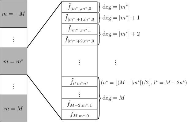
(a) Storage pattern of $\tilde{f}_{lmn}$

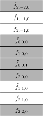
(b) Example: $M=2$

Figure 1: Storage pattern of $\tilde{f}_{lmn}$ showing the two-level structure of the array. The left column of (a) shows that the first-level decomposition of the array (one section for each $m$), and the right column of (a) shows how the elements are stored in the second-level structure. (b) presents an example with $M=2$.

By this storage scheme, for any given $m$, the coefficients associated with the polynomials of degree less than or equal to $M_{0}$ are continuously stored, which makes it easier to perform the matrix-vector multiplication in the numerical algorithm and achieve good cache hit ratio.

3.2.2 Storage of the coefficients $A_{lmn}^{l_{1}m_{1}n_{1},l_{2}m_{2}n_{2}}$

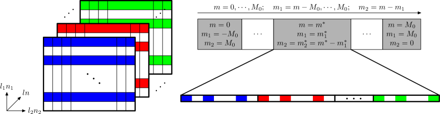
Figure 2: Storage pattern of $A_{lmn}^{l_{1}m_{1}n_{1},l_{2}m_{2}n_{2}}$. The left column shows the three-dimensional view of the coefficients for given $m$, $m_{1}$ and $m_{2}$. The right column gives the general two-level structure of the array.

Similar to the storage of $\tilde{f}_{lmn}$, all the coefficients $A_{lmn}^{l_{1}m_{1}n_{1},l_{2}m_{2}n_{2}}$ are also stored in a continuous array, which can again be considered as the concatenation of a number of sections. Each section contains all the coefficients for given $m$, $m_{1}$ and $m_{2}$. Noting that the range of $m$ is from $0$ to $M_{0}$ while the range of $m_{1}$ and $m_{2}$ is from $-M_{0}$ to $M_{0}$, we can find that the total number of sections is $(3M_{0}+2)(M_{0}+1)/2$. Once $m$ is given, the two indices $l$ and $n$ can be viewed as a one-dimensional index $ln$ by our ordering rule in the storage pattern of $\tilde{f}_{lmn}$. Similarly, $l_{1}n_{1}$ and $l_{2}n_{2}$ can also be regarded as one-dimensional indices. Thus, once $m$, $m_{1}$ and $m_{2}$ are given, the coefficients $A_{lmn}^{l_{1}m_{1}n_{1},l_{2}m_{2}n_{2}}$ can be considered as a three-dimensional array, whose three indices are $ln$, $l_{1}n_{1}$ and $l_{2}n_{2}$ (see the left column of Figure 2). Its storage is a simple flattening the three-dimensional array and is illustrated in the right column of Figure 2.

3.3 Details of the algorithm

Based on the above data structure, the computation of $\tilde{Q}_{lmn}^{*}$ can be implemented very efficiently. The general procedure is as follows:

Algorithm Algorithm to Calculate $\tilde{Q}_{lmn}^{*}$

1:for $m$ from $0$ to $M$ do

2:     if $m>M_{0}$ then

3:         for all $l,n$ satisfying $l\geqslant m$, $l+2n\leqslant M$ do

4:              $\tilde{Q}_{lmn}^{*}\leftarrow-\mu_{M_{0}}\tilde{f}_{lmn}$

5:         end for

6:     else

7:         for all $l,n$ satisfying $l\geqslant m$, $M_{0}<l+2n\leqslant M$ do

8:              $\tilde{Q}_{lmn}^{*}\leftarrow-\mu_{M_{0}}\tilde{f}_{lmn}$

9:         end for

10:         for $m_{1}$ from $m-M_{0}$ to $M_{0}$ do

11:              $m_{2}\leftarrow m-m_{1}$

12:              for all $l,n$ satisfying $l\geqslant m$, $l+2n\leqslant M_{0}$ do

13:                   $\displaystyle\tilde{Q}_{lmn}^{*}\leftarrow\sum_{l_{1}+2n_{1}\leqslant M_{0}}\sum_{l_{2}+2n_{2}\leqslant M_{0}}A_{lmn}^{l_{1}m_{1}n_{1},l_{2}m_{2}n_{2}}\tilde{f}_{l_{1}m_{1}n_{1}}\tilde{f}_{l_{2}m_{2}n_{2}}$

14:              end for

15:         end for

16:     end if

17:end for

18:for all $m=-M,\cdots,-1$ and $l,n$ satisfying $l\geqslant|m|$, $l+2n\leqslant M$ do

19:     $\tilde{Q}_{lmn}^{*}\leftarrow(-1)^{m}\overline{\tilde{Q}_{l,-m,n}^{*}}$

20:end for

It is worth noting that line 10 can be implemented by two matrix-vector multiplications:

$$1: \qquad\tilde{g}_{lmn}^{l_{1}m_{1}n_{1}}=\sum_{l_{2}+2n_{2}\leqslant M_{0}}A_{lmn}^{l_{1}m_{1}n_{1},l_{2}m_{2}n_{2}}\tilde{f}_{l_{2}m_{2}n_{2}},$$ (3.16)

$$2: \qquad\tilde{Q}_{lmn}^{*}=\sum_{l_{1}+2n_{1}\leqslant M_{0}}\tilde{g}_{lmn}^{l_{1}m_{1}n_{1}}\tilde{f}_{l_{1}m_{1}n_{1}}.$$ (3.17)

Using the storage pattern illustrated in Figure 1 and Figure 2, the matrix entries and the vector components involved in the above operations are automatically continuously stored. The details are illustrated in Figure 3. The left column of Figure 3 provides the color coding of the vectors. Each vertical strip denotes the data structure represented on the right column of Figure 1. Since the coefficients with $l+2n\leqslant M_{0}$ and the coefficients with $l+2n>M_{0}$ are treated differently, we distinguish these two parts by shading with slanted lines. The middle column shows the computation of $\tilde{g}_{lmn}^{l_{1}m_{1}n_{1}}$ (equation (3.16)) for given $m$ and $m_{1}$, which is in fact just one matrix-vector multiplication based on our data structure. The color coding of the matrix $A_{lmn}^{l_{1}m_{1}n_{1},l_{2}m_{2}n_{2}}$ is the same as Figure 2. The right column gives the computation of $\tilde{Q}_{lmn}^{*}$, which contains a matrix-vector multiplication (for degree less than or equal to $M_{0}$, equation (3.17)) and a vector scaling (for degree greater than $M_{0}$). The matrix $\tilde{g}_{lmn}^{l_{1}m_{1}n_{1}}$ is a reshaping of the vector in the middle column. By comparing the matrix form and the vector form of $A$ and $\tilde{g}$, one can observe our data structure automatically corresponds to the row-major order of these matrices, which makes it easy to use optimized BLAS libraries such as ATLAS [27] to achieve high numerical efficiency.

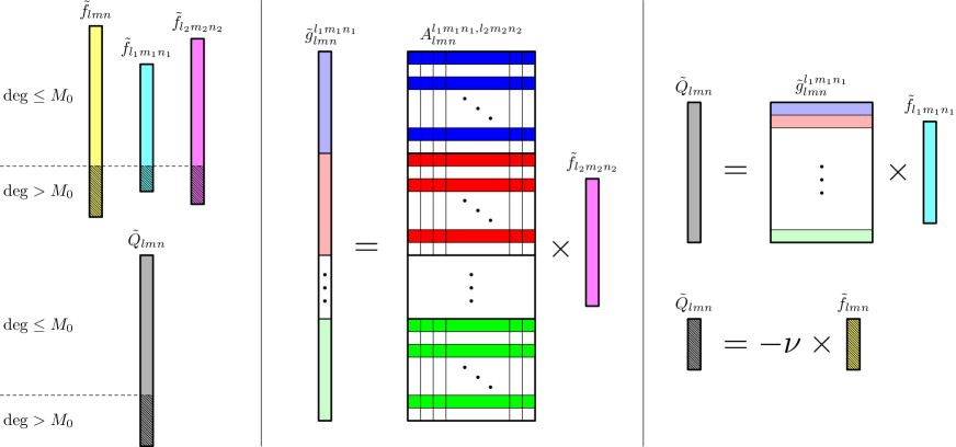
Figure 3: Illustration of the algorithm for given $m$, $m_{1}$ and $m_{2}$.

4 Numerical examples

In this section, we will show some results of our numerical simulation. In all the numerical experiments, we consider the inverse-power-law model, for which the repulsive force between two molecules is proportional to $r^{-\eta}$, with $r$ and $\eta$ being, respectively, the distance between the two molecules and a given positive constant. The details about this model can be found in [4]. In all the tests, we use the classical fourth-order Runge-Kutta method to the equations (2.5) numerically for some given $M_{0}$ and $M$, and the time step is chosen as $\Delta t=0.01$.

For visualization purposes, we define integration operators $\mathcal{I}_{1}:L^{1}(\mathbb{R}^{3})\rightarrow L^{1}(\mathbb{R})$ and $\mathcal{I}_{2}:L^{1}(\mathbb{R}^{3})\rightarrow L^{1}(\mathbb{R}^{2})$ by

$$(\mathcal{I}_{1}f)(v_{1})=\int_{\mathbb{R}}\int_{\mathbb{R}}f(\boldsymbol{v})\,\mathrm{d}v_{2}\,\mathrm{d}v_{3},\qquad\forall f\in L^{1}(\mathbb{R}^{3}),$$

and

$$(\mathcal{I}_{2}f)(v_{1},v_{2})=\int_{\mathbb{R}}f(\boldsymbol{v})\,\mathrm{d}v_{3},\qquad\forall f\in L^{1}(\mathbb{R}^{3}).$$

These 1D and 2D functions are actually marginal distribution functions (MDFs). We will only show the plots for these MDFs due to the difficulty in plotting three-dimensional functions.

Besides, we are also interested in the evolution of the moments of the distribution function, especially the heat flux $q_{i}$ and the stress tensor $\sigma_{ij}$. For a given distribution function $f\in\mathcal{S}$, they are defined as

$$q_{i}=\frac{1}{2}\int_{R^{3}}|\boldsymbol{v}|^{2}v_{i}f(\boldsymbol{v})\,\mathrm{d}\boldsymbol{v},\qquad\sigma_{ij}=\int_{\mathbb{R}^{3}}\left(v_{i}v_{j}-\frac{1}{3}\delta_{ij}|\boldsymbol{v}|^{2}\right)f(\boldsymbol{v})\,\mathrm{d}\boldsymbol{v},\qquad i,j=1,2,3.$$ (4.1)

The relations between these moments and the coefficients are

$$q_{1}=\sqrt{5}{\rm Re}(\tilde{f}_{111}),\quad q_{2}=-\sqrt{5}{\rm Im}(\tilde{f}_{111}),\quad q_{3}=-\sqrt{5/2}\tilde{f}_{101},$$ (4.2)

$$\sigma_{11}=\sqrt{2}{\rm Re}(\tilde{f}_{220})-\tilde{f}_{200}/\sqrt{3},\quad\sigma_{12}=-\sqrt{2}{\rm Im}(\tilde{f}_{220}),\quad\sigma_{13}=-\sqrt{2}{\rm Re}(\tilde{f}_{210}),$$

$$\sigma_{22}=-\sqrt{2}{\rm Re}(\tilde{f}_{220})-\tilde{f}_{200}/\sqrt{3},\quad\sigma_{23}=\sqrt{2}{\rm Im}(\tilde{f}_{210}),\quad\sigma_{33}=2\tilde{f}_{200}/\sqrt{3}.$$

4.1 BKW (Bobylev-Krook-Wu) solution

In this example, we study the Maxwell gas whose the power index $\eta$ equals $5$. In this case, the kernel $B(g,\chi)$ turns out to be independent of $g$ (therefore denoted by $B(\chi)$ below), and it is given in [5, 18] that the spatially homogeneous Boltzmann equation (1.2) admits an exact solution $F(t)=f^{[\tau(t)]}$, where

$$\tau(t)=1-\frac{2}{5}\exp(-\lambda t),\qquad\lambda=\frac{\pi}{2}\int_{0}^{\pi}B(\chi)\sin^{2}\chi\,\mathrm{d}\chi,$$

$$f^{[\tau]}(\boldsymbol{v})=(2\pi\tau)^{-3/2}\exp\left(-\frac{|\boldsymbol{v}|^{2}}{2\tau}\right)\left[1+\frac{1-\tau}{\tau}\left(\frac{|\boldsymbol{v}|^{2}}{2\tau}-\frac{3}{2}\right)\right].$$

The initial MDFs are plotted in Figure 4, in which the contour lines for exact functions and their numerical approximation are hardly distinguishable, with the number $M=20$.

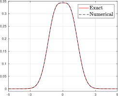
(a) Initial MDF $\mathcal{I}_{1}f^{0}$

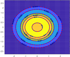
(b) Contours of $\mathcal{I}_{2}f^{0}$

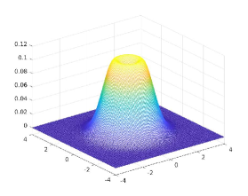
(c) Initial MDF $\mathcal{I}_{2}f^{0}$

Figure 4: Initial marginal distribution functions. In (a), the red line corresponds to the exact solution, while black dashed line corresponds to $M=20$ respectively. In (b), the blue solid lines correspond to the exact solution, and the red dashed lines correspond to the numerical approximation $M=20$. Figure (c) shows only the numerical approximation with $M=20$.

In Figure 5, the marginal distribution functions $\mathcal{I}_{1}F(t)$ at $t=0.2$, $0.4$ and $0.6$ are shown. Here, $M_{0}$ is set as $5$ and $20$. The marginal distribution functions $\mathcal{I}_{2}F(t)$ are plotted in Figures 6 and 7, respectively for $M_{0}=5$ and $20$. For $M_{0}=5$, the numerical solution provides a reasonable approximation, but still has noticeable deviations, while for $M_{0}=20$, the two solutions match perfectly in all cases.

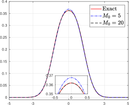
(a) $t=0.2$

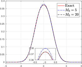
(b) $t=0.4$

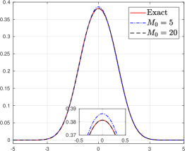
(c) $t=0.6$

Figure 5: Marginal distribution functions $\mathcal{I}_{1}F(t)$ at different times.

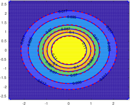
(a) $t=0.2$

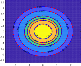
(b) $t=0.4$

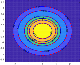
(c) $t=0.6$

Figure 6: Comparison of numerical results using $M_{0}=5$ and the exact solution. The blue contours and the red dashed contours are respectively the results for $M_{0}=5$ and the exact solution.

\begin{overpic}[width=136.5746pt,clip]{ex1_2d_contour_t=02_M0=20_20.pdf} \end{overpic}

(a) $t=0.2$

\begin{overpic}[width=136.5746pt,clip]{ex1_2d_contour_t=04_M0=20_20.pdf} \end{overpic}

(b) $t=0.4$

\begin{overpic}[width=136.5746pt,clip]{ex1_2d_contour_t=06_M0=20_20.pdf} \end{overpic}

(c) $t=0.6$

Figure 7: Comparison of numerical results using $M_{0}=20$ and the exact solution. The blue contours and the red dashed contours are respectively the results for $M_{0}=20$ and the exact solution.

Now we consider the time evolution of the coefficients. By expanding the exact solution into Burnett series, we get the exact solution for the coefficients:

$$\tilde{F}_{lmn}(t)=\left\{\begin{array}[]{ll}\sqrt{\frac{2\Gamma(n+3/2)}{\sqrt{\pi}n!}}(1-n)(1-\tau(t))^{n},&l=m=0,\quad n\in\mathbb{N},\\[13.0pt] 0,&\text{otherwise}.\end{array}\right.$$ (4.3)

Due to the symmetry of the distribution function, the coefficients $\tilde{F}_{lmn}$ are nonzero for any $t$ only when both of $l$ and $m$ are zero. From (4.3), we see that $\tilde{F}_{000}=1$ and $\tilde{F}_{001}=0$ for any $t$. Hence we will focus on the coefficients $\tilde{F}_{00n},n=2,\cdots,5$. For Maxwell molecules, the discrete kernel $A_{lmn}^{l_{1}m_{1}n_{1},l_{2}m_{2}n_{2}}$ is nonzero only when $l+2n=l_{1}+2n_{1}+l_{2}+2n_{2}$. Therefore, for any $M\geqslant M_{0}\geqslant 10$, the numerical results for these coefficients are exactly the same (regardless of round-off errors), and we just show the results for $M_{0}=M=20$ here. Figure 8 gives the comparison between the numerical solution and the exact solution for these coefficients. In all plots, the two lines almost coincide with each other.

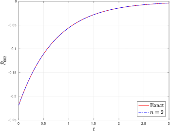
(a) $\tilde{F}_{002}(t)$

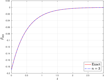
(b) $\tilde{F}_{003}(t)$

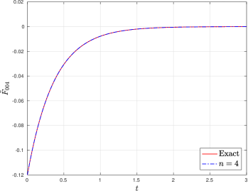
(c) $\tilde{F}_{004}(t)$

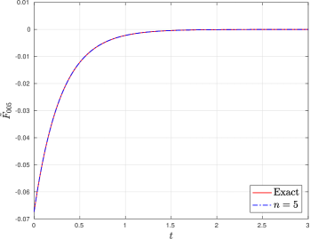
(d) $\tilde{F}_{005}(t)$

Figure 8: The evolution of the coefficients. The red lines correspond to the reference solution, and the blue dashed lines correspond to the numerical solution.

4.2 Quadruple-Gaussian initial data

In this example, we perform the numerical test for the hard potential case where the power index $\eta$ equals $10$. The initial distribution function is

$$f^{0}(\boldsymbol{v})=\frac{1}{4\pi^{3/2}}\left[\exp\Big{(}-\frac{(v_{1}+u)^{2}+v_{2}^{2}+v_{3}^{2}}{2\theta}\Big{)}+\exp\Big{(}-\frac{(v_{1}-u)^{2}+v_{2}^{2}+v_{3}^{2}}{2\theta}\Big{)}\right.$$ (4.4)

$$\left.+\exp\Big{(}-\frac{v_{1}^{2}+(v_{2}+u)^{2}+v_{3}^{2}}{2\theta}\Big{)}+\exp\Big{(}-\frac{v_{1}^{2}+(v_{2}-u)^{2}+v_{3}^{2}}{2\theta}\Big{)}\right],$$

where $u=\sqrt{2}$ and $\theta=1/3$. In all our numerical tests, we use $M=40$, which gives a good approximation of the initial distribution function (see Figure 9).

\begin{overpic}[width=127.46777pt,clip]{ex2_1d_t=0.pdf} \end{overpic}

(a) Initial MDF $\mathcal{I}_{1}f^{0}$

\begin{overpic}[width=136.5746pt,clip]{ex2_2d_contour_t=0.pdf} \end{overpic}

(b) Contours of $\mathcal{I}_{2}f^{0}$

\begin{overpic}[width=145.68143pt,clip]{ex2_2d_t=0.pdf} \end{overpic}

(c) Initial MDF $\mathcal{I}_{2}f^{0}$

Figure 9: Initial marginal distribution functions. In (a), the red line corresponds to the exact solution, while black dashed line corresponds to $M=40$ respectively. In (b), the blue solid lines correspond to the exact solution, and the red dashed lines correspond to the numerical approximation $M=40$. Figure (c) shows only the numerical approximation $M=40$.

For this example, we set the numerical result with $M_{0}=20$ as the reference solution. The numerical results for $M_{0}=5$, $10$, $15$ are given respectively in Figure 10, 11, and 12. For each $M_{0}$, the marginal distribution functions $\mathcal{I}_{2}F(t)$ at $t=0.1$, $0.2$ and $0.3$ are shown.

Due to the high nonequilibrium of this example, when $M_{0}=5$ and $10$, the “size” of the quadratic part in the collision term is too small to describe the evolution of the distribution function, while the numerical results for $M_{0}=15$ and $M_{0}=20$ agree well with each other (except the central area for $t=0.1$, where the distribution function is very flat). This indicates the observation of numerical convergence, meaning that $M_{0}=15$ is sufficient to describe the evolution of the distribution function. This example is a harder version of the bi-Gaussian initial data used in [25] for Hermite basis functions, and therefore requires more degrees of freedom to give satisfactory numerical results. However, as will be shown later, by using Burnett basis functions, the computational cost for $M_{0}=20$ is even smaller than the computational cost for $M_{0}=15$ using Hermite basis functions, even if the results are essentially identical.

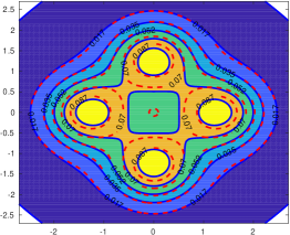
(a) $t=0.1$

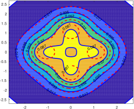
(b) $t=0.2$

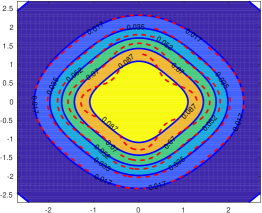
(c) $t=0.3$

Figure 10: Comparison of numerical results using $M_{0}=5$ and $M_{0}=20$. The blue contours and the red dashed contours are respectively the results for $M_{0}=5$ and $M_{0}=20$.

\begin{overpic}[width=136.5746pt,clip]{ex2_2d_contour_t=01_M0=10_40.pdf} \end{overpic}

(a) $t=0.1$

\begin{overpic}[width=136.5746pt,clip]{ex2_2d_contour_t=02_M0=10_40.pdf} \end{overpic}

(b) $t=0.2$

\begin{overpic}[width=136.5746pt,clip]{ex2_2d_contour_t=03_M0=10_40.pdf} \end{overpic}

(c) $t=0.3$

Figure 11: Comparison of numerical results using $M_{0}=10$ and $M_{0}=20$. The blue contours and the red dashed contours are respectively the results for $M_{0}=10$ and $M_{0}=20$.

\begin{overpic}[width=136.5746pt,clip]{ex2_2d_contour_t=01_M0=15_40.pdf} \end{overpic}

(a) $t=0.1$

\begin{overpic}[width=136.5746pt,clip]{ex2_2d_contour_t=02_M0=15_40.pdf} \end{overpic}

(b) $t=0.2$

\begin{overpic}[width=136.5746pt,clip]{ex2_2d_contour_t=03_M0=15_40.pdf} \end{overpic}

(c) $t=0.3$

Figure 12: Comparison of numerical results using $M_{0}=15$ and $M_{0}=20$. The blue contours and the red dashed contours are respectively the results for $M_{0}=15$ and $M_{0}=20$.

Now we consider the evolution of the moments. In this example, the stress tensor and heat flux satisfy $\sigma_{11}=\sigma_{22}=-0.5\sigma_{33}$ and $q_{i}=0,i=1,2,3$. Therefore, we focus only on the evolution of $\sigma_{11}$, which is plotted in Figure 13. It can be seen that the four tests give almost identical results. Even for $M_{0}=5$ and $10$, while the distribution functions are not approximated very well, the evolution of the stress tensor is very accurate.

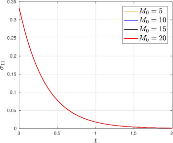
Figure 13: Evolution of $\sigma_{11}(t)$. Four lines are on top of each other.

4.3 Discontinuous initial data

In this example, we reconsider the problem with the same discontinuous initial condition as in [25]:

$$f^{0}(\boldsymbol{v})=\left\{\begin{array}[]{ll}\dfrac{\sqrt[4]{2}(2-\sqrt{2})}{\pi^{3/2}}\exp\left(-\dfrac{|\boldsymbol{v}|^{2}}{\sqrt{2}}\right),&\text{if }v_{1}>0,\\[10.0pt] \dfrac{\sqrt[4]{2}(2-\sqrt{2})}{4\pi^{3/2}}\exp\left(-\dfrac{|\boldsymbol{v}|^{2}}{2\sqrt{2}}\right),&\text{if }v_{1}<0.\end{array}\right.$$

In [25], the authors used Hermite spectral method to do the computation up to $M_{0}=15$, which still shows significant difference in the numerical results compared with $M_{0}=10$. In this paper, we are going to confirm the reliability of the results obtained with $M_{0}=15$. As in [25], we only focus on the evolution of the moments. The numerical results for the hard potential $\eta=10$ and soft potential $\eta=3.1$ with different choices of $M_{0}$ and $M$ are shown in Figure 14. For $\eta=3.1$, the horizontal axes are the scaled time $t_{s}=t/\tau$ with $\tau\approx 2.03942$ as in [25], so that the two models have the same mean relaxation time near equilibrium.

Since for the homogeneous Boltzmann equation, the behaviors of stress tensor and heat flux are the same for any $M\geqslant M_{0}\geqslant 3$, we let $M=M_{0}=5$, $10$, $15$ and $20$, and the results are plotted in Figure 14. The numerical results for $M_{0}=5$, $10$ and $15$ are exactly the same as [25]. However, due to the significant enhancement of computational efficiency, we can get the results for $M_{0}=20$, and the results are almost the same as those for $M_{0}=15$, which indicates that they should be very close to the exact solution. The whole pictures of $\sigma_{11}$ and $\sigma_{22}$ show much clearer converging trend of the numerical solutions with increasing $M_{0}$, compared with the numerical results in [25] where the profiles for $M_{0}=20$ was not present. For the heat flux $q_{1}$, not surprisingly, the four results are hardly distinguishable.

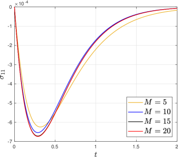
(a) $\sigma_{11}(t)$ ($\eta=10$)

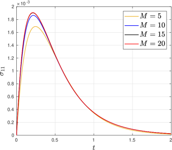
(b) $\sigma_{11}(t)$ ($\eta=3.1$)

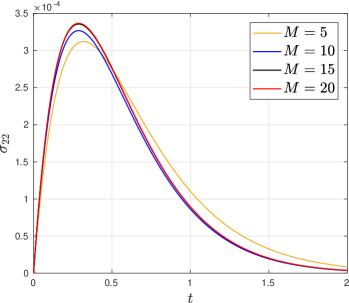
(c) $\sigma_{22}(t)$ ($\eta=10$)

(d) $\sigma_{22}(t)$ ($\eta=3.1$)

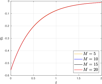
(e) $q_{1}(t)$ ($\eta=10$)

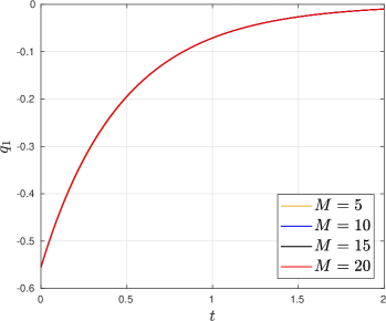
(f) $q_{1}(t)$ ($\eta=3.1$)

Figure 14: Evolution of the stress and the heat flux. The left column shows the results for $\eta=10$, and the right column shows the results for $\eta=3.1$. In the right column, the horizontal axes are the scaled time.

Finally, the computational time for one evaluation of the quadratic collision term under the framework of Burnett series and Hermite series [25] is plotted in Figure 15. Here, the number $M$ is fixed as $M=20$, and $M_{0}$ increases from $5$ to $20$. It is clear that the computational cost is greatly reduced by using Burnett basis functions, especially when $M$ is large.

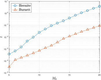
Figure 15: Comparison of the computational time for one evaluation of the collision operator using the method in this paper and that in [25]. $M$ is fixed as $M=20$ and $M_{0}$ changes from $5$ to $20$. The $x$-axis is $M_{0}$ and the $y$-axis is the logarithm of the computational time.

5 Proof of theorems

In this section, we prove the three theorems in Section 2. Firstly, we introduce two lemmas as following:

Lemma 4.

Let $\mathbf{R}$ be an $3\times 3$ orthogonal matrix. Define the rotation operator $\mathcal{R}$ by

$$(\mathcal{R}f)(\boldsymbol{v})=f(\mathbf{R}\boldsymbol{v}),\qquad\forall f:\mathbb{R}^{3}\rightarrow\mathbb{C}.$$

Then when $\mathcal{Q}[f,g]$ is well-defined for some functions $f$ and $g$, we have $\mathcal{Q}[f,g](\mathbf{R}\boldsymbol{v})=\mathcal{Q}[\mathcal{R}f,\mathcal{R}g](\boldsymbol{v})$.

Lemma 5.

Talmi coefficient $\left(\begin{array}[]{c|c}l_{1}m_{1}n_{1}&l_{3}m_{3}n_{3}\\ l_{2}m_{2}n_{2}&l_{4}m_{4}n_{4}\end{array}\right)$ is zero if

$$l_{1}+2n_{1}+l_{2}+2n_{2}\neq l_{3}+2n_{3}+l_{4}+2n_{4}.$$ (5.1)

The first lemma is a well-known result and we are not going to prove it in this paper. The proof of the second lemma can be find in [19, page 135-137]. Now we start to prove the theorems.

Proof of Theorem 1.

For any $\eta\in\mathbb{R}$, we define the rotation matrix

$$\mathbf{R}_{\eta}=\begin{pmatrix}\cos\eta&-\sin\eta&0\\ \sin\eta&\cos\eta&0\\ 0&0&1\end{pmatrix}.$$

Using spherical coordinates $\boldsymbol{v}=(r\sin\theta\cos\phi,r\sin\theta\sin\phi,r\cos\theta)^{T}$, one can see that

$$\mathbf{R}_{\eta}\boldsymbol{v}=(r\sin\theta\cos(\phi+\eta),r\sin\theta\sin(\phi+\eta),r\cos\theta)^{T}.$$

Therefore

$$p_{lmn}(\mathbf{R}_{\eta}\boldsymbol{v})=\mathrm{e}^{\mathrm{i}m\eta}p_{lmn}(\boldsymbol{v}),\qquad\varphi_{lmn}(\mathbf{R}_{\eta}\boldsymbol{v})=\mathrm{e}^{\mathrm{i}m\eta}\varphi_{lmn}(\boldsymbol{v}).$$

Let $\mathcal{R}_{\eta}$ be the rotation operator such that $(\mathcal{R}_{\eta}f)(\boldsymbol{v})=f(\mathbf{R}_{\eta}\boldsymbol{v})$. Now we can rewrite (2.3) as

$$\begin{split}A_{lmn}^{l_{1}m_{1}n_{1},l_{2}m_{2}n_{2}}&=\int_{\mathbb{R}^{3}}\overline{p_{lmn}(\mathbf{R}_{\eta}\boldsymbol{v})}\mathcal{Q}[\varphi_{l_{1}m_{1}n_{1}},\varphi_{l_{2}m_{2}n_{2}}](\mathbf{R}_{\eta}\boldsymbol{v})\,\mathrm{d}\boldsymbol{v}\\ &=\int_{\mathbb{R}^{3}}\mathrm{e}^{-\mathrm{i}m\eta}\overline{p_{lmn}(\boldsymbol{v})}\mathcal{Q}[\mathcal{R}_{\eta}\varphi_{l_{1}m_{1}n_{1}},\mathcal{R}_{\eta}\varphi_{l_{2}m_{2}n_{2}}](\boldsymbol{v})\,\mathrm{d}\boldsymbol{v}\\ &=\mathrm{e}^{\mathrm{i}(m_{1}+m_{2}-m)\eta}\int_{\mathbb{R}^{3}}\overline{p_{lmn}(\boldsymbol{v})}\mathcal{Q}[\varphi_{l_{1}m_{1}n_{1}},\varphi_{l_{2}m_{2}n_{2}}](\boldsymbol{v})\,\mathrm{d}\boldsymbol{v}\\ &=\mathrm{e}^{\mathrm{i}(m_{1}+m_{2}-m)\eta}A_{lmn}^{l_{1}m_{1}n_{1},l_{2}m_{2}n_{2}}.\end{split}$$ (5.2)

Here we have used the rotational invariance and bilinearity of the collision operator $\mathcal{Q}[\cdot,\cdot]$. Note that (5.2) holds for any $\eta$. If $m\neq m_{1}+m_{2}$, this shows that $A_{lmn}^{l_{1}m_{1}n_{1},l_{2}m_{2}n_{2}}=0$. ∎

Proof of Theorem 2.

Since $B(g,\chi)=\sigma(\chi)$ is independent of $g$, in (3.2), the integrals with respect to $g$ and $\chi$ can be split:

$$\begin{split}V_{nn^{\prime}}^{l}&=\frac{1}{16\sqrt{2}\pi^{5/2}}\sqrt{\frac{n!n^{\prime}!}{\Gamma(n+l+3/2)\Gamma(n^{\prime}+l+3/2)}}\int_{0}^{\pi}\sigma(\chi)[(2l+1)^{2}P_{l}(\cos\chi)-1]\,\mathrm{d}\chi\times{}\\ &\qquad\int_{0}^{+\infty}\left(\frac{g^{2}}{4}\right)^{l+1}L_{n}^{(l+1/2)}\left(\frac{g^{2}}{4}\right)L_{n^{\prime}}^{(l+1/2)}\left(\frac{g^{2}}{4}\right)\exp\left(-\frac{g^{2}}{4}\right)\,\mathrm{d}g,\end{split}$$ (5.3)

which vanishes if $n\neq n^{\prime}$, due to the orthogonality of Laguerre polynomials. Hence, using Lemma 5, we can obtain that the summands in (3.1) do not vanish only if

$$n_{4}=n_{4}^{\prime},\quad l_{3}+2n_{3}+l_{4}+2n_{4}^{\prime}=l+2n,\quad l_{3}+2n_{3}+l_{4}+2n_{4}=l_{1}+2n_{1}+l_{2}+2n_{2}.$$

Direct simplification yields the conclusion in the theorem. ∎

Proof of Theorem 3.

Set $\mathbf{R}=\operatorname{diag}\{1,-1,1\}$, then using the same approach as that in the proof of Theorem 1, one can directly prove this theorem. ∎

6 Conclusion

This work aims to model and simulate the binary collision between gas molecules under the framework of the Burnett polynomials. The special sparsity of the coefficients is fully utilized, and we have proposed a method to compute the coefficients in the spectral expansion with high accuracy based on the work [25]. Moreover, the data structure and the implementation of the algorithm are carefully designed to achieve high numerical efficiency.

In order to provide further flexibility, especially when taking into account the spatial inhomogeneity, we employ the modelling technique used in [8, 25], where the quadratic form is preserved only for the first few moments. It is validated again that the method is efficient in capturing the evolution of lower-order moments. The implementation of the spatially inhomogeneous Boltzmann equation is in progress.

References

- [1] A. Alekseenko and E. Josyula. Deterministic solution of the spatially homogeneous Boltzmann equation using discontinuous Galerkin discretizations in the velocity space. J. Comput. Phys., 272:170–188, 2014.
- [2] M. M. Bakri. A simplified expression for the Talmi coefficients. Nucl. Phys., 96(1):115–120, 1967.
- [3] G. A. Bird. Approach to translational equilibrium in a rigid sphere gas. Phys. Fluids, 6(10):1518–1519, 1963.
- [4] G. A. Bird. Molecular Gas Dynamics and the Direct Simulation of Gas Flows. Oxford: Clarendon Press, 1994.
- [5] A. V. Bobylev. Exact solutions of the nonlinear Boltzmann equation and the theory of relaxation of a Maxwellian gas. Theor. Math. Phys., 60(2):820–841, 1984.
- [6] D. Burnett. The distribution of molecular velocities and the mean motion in a non-uniform gas. Proc. London Math. Soc., 40(1):382–435, 1936.
- [7] Z. Cai, Y. Fan, and L. Ying. An entropic fourier method for the Boltzmann equation. SIAM J. Sci. Comput., 40(5):A2858–A2882, 2018.
- [8] Z. Cai and M. Torrilhon. Approximation of the linearized Boltzmann collision operator for hard-sphere and inverse-power-law models. J. Comput. Phys., 295:617–643, 2015.
- [9] Z. Cai and M. Torrilhon. Numerical simulation of microflows using moment methods with linearized collision operator. J. Sci. Comput., 74(1):336–374, 2018.
- [10] G. Dimarco, R. Loubére, J. Narski, and T. Rey. An efficient numerical method for solving the Boltzmann equation in multidimensions. J. Comput. Phys., 353:46–81, 2018.
- [11] Francis Filbet, Lorenzo Pareschi, and Thomas Rey. On steady-state preserving spectral methods for homogeneous boltzmann equations. Comptes Rendus Mathematique, 353(4):309–314, 2015.
- [12] I. M. Gamba, J. R. Haack, C. D. Hauck, and J. Hu. A fast spectral method for the Boltzmann collision operator with general collision kernels. SIAM J. Sci. Comput., 39(4):B658–B674, 2017.
- [13] I. M. Gamba and S. Rjasanow. Galerkin-Petrov approach for the Boltzmann equation. J. Comput. Phys., 366:341–365, 2018.
- [14] I. M. Gamba and S. H. Tharkabhushanam. Spectral-Lagrangian methods for collisional models of non-equilibrium statistical states. J. Comput. Phys., 228(6):2012–2036, 2009.
- [15] H. Grad. On the kinetic theory of rarefied gases. Comm. Pure Appl. Math., 2(4):331–407, 1949.
- [16] H. Grad. Principles of the kinetic theory of gases. Handbuch der Physik, 12:205–294, 1958.
- [17] Z. Hu, Z. Cai, and Y. Wang. Numerical simulation of microflows using Hermite spectral methods. arXiv:1807.06236, 2018. submitted.
- [18] Max Krook and Tai Tsun Wu. Exact solutions of the boltzmann equation. The Physics of Fluids, 20(10):1589–1595, 1977.
- [19] K. Kumar. Polynomial expansions in kinetic theory of gases. Ann. Phys., 37:113–141, 1966.
- [20] C. Mouhot and L. Pareschi. Fast algorithms for computing the Boltzmann collision operator. Math. Comp., 75(256):1833–1852, 2006.
- [21] C. Mouhot, L. Pareschi, and T. Rey. Convolutive decomposition and fast summation methods for discrete-velocity approximations of the Boltzmann equation. ESAIM: M2AN, 47(5):1515–1531, 2013.
- [22] L. Pareschi and B. Perthame. A Fourier spectral method for homogeneous Boltzmann equations. Transport Theor. Stat., 25(3-5):369–382, 1996.
- [23] L. Pareschi and G. Russo. On the stability of spectral methods for the homogeneous Boltzmann equation. Trans. Theory Stat. Phys., 29(3–5):431–447, 2000.
- [24] I. Talmi. Nuclear spectroscopy with harmonic oscillator wave-functions. Helv. Phys. Acta, 25(3):185–234, 1952.
- [25] Y. Wang and Z. Cai. Approximation of the Boltzmann collision operator based on Hermite spectral method. arXiv:1803.11191, 2018. submitted.
- [26] C. S. Wang Chang and G. E. Uhlenbeck. On the propagation of sound in monatomic gas. Technical report, Engineering Research Insitute, University of Michigan, Ann Arbor, 1952.
- [27] R. C. Whaley, A. Petitet, and J. J. Dongarra. Automated empirical optimizations of software and the atlas project. Parallel Computing, 27(1–2):3–35, 2001.
- [28] L. Wu, J. Reese, and Y. Zhang. Solving the Boltzmann equation deterministically by the fast spectral method: Application to gas microflows. J. Fluid Mech., 746:53–84, 2014.
- [29] L. Wu, C. White, T. Scanlona, J. Reese, and Y. Zhang. Deterministic numerical solutions of the Boltzmann equation using the fast spectral method. J. Comput. Phys., 250:27–52, 2013.