Lattice Boltzmann approach to rarefied gas flows using half-range Gauss-Hermite quadratures: Comparison to DSMC results based on ab initio potentials

Abstract

In this paper, we employ the lattice Boltzmann method to solve the Boltzmann equation with the Shakhov model for the collision integral in the context of the 3D planar Couette flow. The half-range Gauss-Hermite quadrature is used to account for the wall-induced discontinuity in the distribution function. The lattice Boltzmann simulation results are compared with direct simulation Monte Carlo (DSMC) results for ${}^{3}{\rm He}$ and ${}^{4}{\rm He}$ atoms interacting via ab initio potentials, at various values of the rarefaction parameter $\delta$, where the temperature of the plates varies from $1\ {\rm K}$ up to $3000\ {\rm K}$. Good agreement is observed between the results obtained using the Shakhov model and the DSMC data at large values of the rarefaction parameter. The agreement deteriorates as the rarefaction parameter is decreased, however we highlight that the relative errors in the non-diagonal component of the shear stress do not exceed $2.5\%$.

I INTRODUCTION

The main difficulty in simulating steady-state rarefied channel flows is caused by the discontinuity in the distribution function induced by the particle-wall interaction. A generally accepted method for the simulation of rarefied flows is the Direct Simulation Monte Carlo (DSMC) method. Although accurate, DSMC simulations are computationally demanding, particularly in the hydrodynamic and transition regimes. A convenient alternative to DSMC is the Boltzmann equation with a suitable model (e.g., BGK bhatnagar54 or Shakhov shakhov68a ) for the collision term sharipov16 . Various numerical methods have been developed to solve such model equations, including the Discrete Velocity Method (DVM) sharipov16 , the Discrete Unified Gas Kinetic Scheme (DUGKS) guo13 , the discrete Boltzmann models xu18 and the lattice Boltzmann (LB) models ambrus16jcp .

Close to the hydrodynamic regime, reliable results can be obtained using lattice Boltzmann models based on the D3Q27 model yudistiawan10 , the spherical decomposition of the velocity space ambrus12pre or the full-range Gauss-Hermite quadrature ambrus16jcp ; meng13jfm . As the degree of rarefaction increases, the number of velocities required by such models to ensure accurate results increases significantly ambrus16jcp ; ambrus12pre ; piaud14ijmpc ; ambrus16jocs . This is due to the discontinuity of the distribution function, which develops due to the particle-wall interaction gross57 ; takata13 . When the gas is far from equilibrium, this discontinuity can be managed more efficiently with LB models based on half-range Gauss-Hermite quadratures. As demonstrated in the context of the Couette flow between parallel plates ambrus16jcp ; ambrus16jocs , the ratio between the number of velocities used when full-range or half-range Gauss-Hermite quadratures are employed on the Cartesian axis perpendicular to the wall increases dramatically for values of the Knudsen number ${\rm Kn}$ exceeding $0.1$ (e.g., at ${\rm Kn}=0.5$, this ratio is $9.5$).

In this contribution, we validate our LB simulation results by comparison to the DSMC results reported in Ref. sharipov18 , which were obtained for dilute gases comprised of ${}^{3}{\rm He}$ and ${}^{4}{\rm He}$ atoms that interact via quantum scattering cross-sections, computed using ab initio potentials. The connection between the Shakhov model employed in the LB method and the interaction model employed in the DSMC method is made by implementing the relaxation time $\tau$ and the Prandtl number ${\rm Pr}$ such that the viscosity $\mu$ and heat conductivity $\kappa$ match the values computed in Ref. cencek12 .

The paper is structured as follows. First, the application of the Shakhov model with reduced distributions for the simulation of gases with interparticle interactions based on ab initio potentials is discussed. Next, we introduce the mixed quadrature LB models, which employ the half-range Gauss-Hermite quadrature on the axis perpendicular to the wall. The comparison of the numerical results obtained using the Shakhov collision model and the full DSMC analysis is further discussed. Finally, we present our conclusions.

II SHAKHOV KINETIC MODEL FOR THE COUETTE FLOW

In this paper, we focus on the study of the Couette flow between parallel plates. The coordinate system is chosen such that the $x$ axis is perpendicular to the walls. The origin of the coordinate system is taken to be on the channel centerline, such that the left and right walls are located at $x=-L/2$ and $x=L/2$, respectively. The plates are set in motion along the $y$ axis and the flow is studied in the Galilean frame where the left and right plates move with velocities $-u_{w}$ and $u_{w}$, respectively. Both plates are kept at constant temperature $T_{w}$. In this case, the Boltzmann equation with the Shakhov approximation for the collision term can be written as follows shakhov68a ; ambrus12pre ; ambrus18pre :

$$\frac{\partial f}{\partial t}+\frac{p_{x}}{m}\partial_{x}f=-\frac{1}{\tau}\left[f-f^{\rm{(eq)}}(1+\mathbb{S})\right],$$ (1)

where $f$ is the particle distribution function, $p_{x}$ is the particle momentum along the direction perpendicular to the walls, $m$ is the particle mass and $\tau$ is the relaxation time. The Maxwell-Boltzmann distribution function $f^{\rm{(eq)}}$ for the ideal gas is:

$$f^{\rm{(eq)}}=ng(p_{x},u_{x},T)g(p_{y},u_{y},T)g(p_{z},u_{z},T),\qquad g(p,u,T)=\frac{1}{\sqrt{2\pi mK_{B}T}}e^{-(p-mu)^{2}/2mK_{B}T},$$ (2)

where $u_{\alpha}$ is the macroscopic velocity along the $\alpha$ direction ($\alpha\in\{x,y,z\}$), while $n$ and $T$ are the particle number density and the local temperature, respectively. The Shakhov term $\mathbb{S}$ is given by:

$$\mathbb{S}=\frac{1-{\rm Pr}}{nK_{B}^{2}T^{2}}\left(\frac{\bm{\xi}^{2}}{5mK_{B}T}-1\right)\bm{q}\cdot\bm{\xi},\vspace{-5pt}$$ (3)

where $\xi_{\alpha}=p_{\alpha}-mu_{\alpha}$ and $q_{\alpha}$ are the $\alpha$ components of the peculiar velocity and heat flux vectors. The Prandtl number ${\rm Pr}=c_{p}\mu/\kappa$, where $c_{p}=5K_{B}/2m$, represents a free parameter of the Shakhov model. This parameter can be used to tune the heat conductivity $\kappa$, while the viscosity is proportional to the relaxation time $\tau$ and is given by $\mu=\tau P$, where $P=nK_{B}T$ is the ideal gas pressure.

Since the flow properties are trivial along the $z$ direction, it is convenient to introduce the reduced distributions $\phi$ and $\chi$ through li04 ; meng13jcp :

$$\phi=\int_{-\infty}^{\infty}dp_{z}\,f,\qquad\chi=\int_{-\infty}^{\infty}dp_{z}\frac{p_{z}^{2}}{m}\,f.$$ (4)

The equations obeyed by the reduced distributions $\phi$ and $\chi$ can be obtained by multiplying Eq. (1) with $1$ and $p_{z}^{2}/m$ and integrating over $p_{z}$:

$$\frac{\partial}{\partial t}\left(\begin{array}[]{c}\phi\\ \chi\end{array}\right)+\frac{p_{x}}{m}\frac{\partial}{\partial x}\left(\begin{array}[]{c}\phi\\ \chi\end{array}\right)=-\frac{1}{\tau}\left[\begin{array}[]{c}\phi-\phi^{\rm(eq)}(1+\mathbb{S}_{\phi})\\ \chi-\chi^{\rm(eq)}(1+\mathbb{S}_{\chi})\end{array}\right],$$ (5)

where $\phi^{\rm(eq)}=ng(p_{x},u_{x},T)g(p_{y},u_{y},T)$, $\chi^{\rm(eq)}=K_{B}T\phi^{\rm(eq)}$ and the Shakhov terms $\mathbb{S}_{\phi}$ and $\mathbb{S}_{\chi}$ are given by:

$$\mathbb{S}_{\phi}=\frac{1-{\rm Pr}}{nK_{B}^{2}T^{2}}\left(\frac{\xi_{x}^{2}+\xi_{y}^{2}}{5mK_{B}T}-\frac{4}{5}\right)(q_{x}\xi_{x}+q_{y}\xi_{y}),\qquad\mathbb{S}_{\chi}=\frac{1-{\rm Pr}}{nK_{B}^{2}T^{2}}\left(\frac{\xi_{x}^{2}+\xi_{y}^{2}}{5mK_{B}T}-\frac{2}{5}\right)(q_{x}\xi_{x}+q_{y}\xi_{y}).$$ (6)

The macroscopic quantities describing the fluid can be obtained as moments of $\phi$ and $\chi$, as follows:

$$\left(\begin{array}[]{c}n\\ u_{i}\\ T_{ij}\end{array}\right)=\int dp_{x}dp_{y}\left(\begin{array}[]{c}1\\ p_{i}/\rho\\ \xi_{i}\xi_{j}/m\end{array}\right)\phi,\qquad T_{zz}=\int dp_{x}dp_{y}\,\chi,$$ (13)

$$\left(\begin{array}[]{c}q_{x}\\ q_{y}\end{array}\right)=\int dp_{x}dp_{y}\left[\left(\begin{array}[]{c}(\xi_{x}^{2}+\xi_{y}^{2})\xi_{x}/2m^{2}\\ (\xi_{x}^{2}+\xi_{y}^{2})\xi_{y}/2m^{2}\end{array}\right)\phi+\left(\begin{array}[]{c}\xi_{x}/2m\\ \xi_{y}/2m\end{array}\right)\chi\right],$$ (20)

where $i,j$ take values in $\{x,y\}$, while $u_{z}=T_{xz}=T_{yz}=q_{z}=0$. The temperature is obtained via $T=\frac{1}{3nK_{B}}(T_{xx}+T_{yy}+T_{zz})$.

Due to the symmetries of Eq. (5), $\phi(-x,-p_{x},-p_{y})=\phi(x,p_{x},p_{y})$ and $\chi(-x,-p_{x},-p_{y})=\chi(x,p_{x},p_{y})$ for $0\leq x\leq L/2$, such that only the right half of the channel can be considered. At $x=L/2$, diffuse reflection boundary conditions are imposed:

$$\phi(x=L/2,p_{x}<0) = n_{w}g(p_{x},0,T_{w})g(p_{y},u_{w},T_{w}),$$

$$\chi(x=L/2,p_{x}<0) = n_{w}K_{B}T_{w}g(p_{x},0,T_{w})g(p_{y},u_{w},T_{w}),$$ (21)

where $n_{w}$ is obtained by imposing zero mass flux through the wall:

$$n_{w}=-\frac{\displaystyle\int_{0}^{\infty}dp_{x}\int_{-\infty}^{\infty}dp_{y}\,\phi(x=L/2)\,p_{x}}{\displaystyle\int_{-\infty}^{0}dp_{x}\int_{-\infty}^{\infty}dp_{y}\,g(p_{x},0,T_{w})g(p_{y},u_{w},T_{w})p_{x}}.$$ (22)

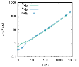
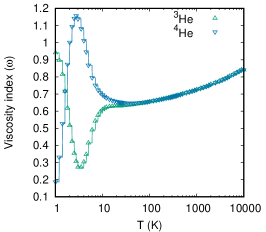
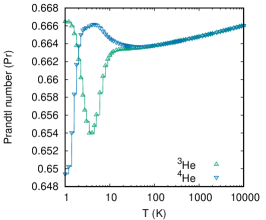
Figure 1: Temperature dependence of (a) dynamic viscosity $\mu$ (in $\mu{\rm Pa}\cdot s$); (b) viscosity index $\omega$; and (c) Prandtl number ${\rm Pr}$, as given by Eqs. (24) and (25). In (a), the tabulated values cencek12 for the viscosity are shown using hollow circles, while the continuous lines correspond to the piecewise functions defined in Eq. (24). The viscosity index and Prandtl number are shown as piecewise constant functions, while the symbols mark the values obtained via the tabulated data from Ref. cencek12 .

The connection between the relaxation time approximation of the Boltzmann equation and the full collision integral for a given interaction model can be made at the level of the transport coefficients. For simple interaction models such as the hard-sphere or Maxwell molecules gases, the viscosity has a temperature dependence of the form

$$\mu=\mu_{\rm ref}(T/T_{\rm ref})^{\omega},$$ (23)

where the viscosity index $\omega$ takes the values $1/2$ and $1$ for hard sphere and Maxwell molecules, respectively. For real gases, $\omega$ is in general temperature-dependent. In the contex of interactions based on ab initio potentials, the viscosity $\mu$ was tabulated for gases comprised of ${}^{3}{\rm He}$ and ${}^{4}{\rm He}$ atoms in the supplementary materials of Ref. cencek12 . In this work, we employ Eq. (23) in a piecewise fashion by determining appropriate values of $\omega$ in order to interpolate the tabulated data, as follows. Considering that the data table contains $N$ entries, let $\mu_{n}$ and $\mu_{n+1}$ ($1\leq n<N$) represent two consecutive values of the viscosity, corresponding to the values $T_{n}$ and $T_{n+1}$ of the temperature. For the interval $T\in[T_{n},T_{n+1}]$, Eq. (23) is replaced by:

$$\mu^{(n)}(T)=\mu_{n}(T/T_{n})^{\omega_{n}},\qquad\omega_{n}=\frac{\ln(\mu_{n+1}/\mu_{n})}{\ln(T_{n+1}/T_{n})},\vspace{-5pt}$$ (24)

such that $\mu^{(n)}(T_{n})=\mu_{n}$ and $\mu^{(n)}(T_{n+1})=\mu_{n+1}$. We also take advantage of the freedom in controlling the Prandtl number ${\rm Pr}$ via the Shakhov collision model in order to track the (small) variations of ${\rm Pr}$ with temperature. For simplicity, we consider a piecewise constant implementation of ${\rm Pr}$, such that ${\rm Pr}={\rm Pr}_{n}$ when $T_{n}\leq T<T_{n+1}$, where ${\rm Pr}_{n}=c_{p}\mu_{n}/\kappa_{n}$ is obtained using the tabulated value $\kappa_{n}$ of the heat conductivity corresponding to $T=T_{n}$. In order to access temperature ranges outside the tabulated data, Eq. (23) is extrapolated by taking $\mu(T)=\mu^{(1)}(T)$ and ${\rm Pr}(T)={\rm Pr}_{1}$ for $T<T_{2}$, while $\mu(T)=\mu^{(N-1)}(T)$ and ${\rm Pr}(T)={\rm Pr}_{N}$ for $T>T_{N}$. The mathematical expression for the above algorithm is:

$$\mu(T)=\left\{\begin{array}[]{lll}\mu^{(1)}(T),&&T<T_{2},\\ \mu^{(n)}(T),&&T_{n}<T<T_{n+1},\\ \mu^{(N-1)}(T),&&T_{N}<T,\end{array}\right.\qquad{\rm Pr}(T)=\left\{\begin{array}[]{lll}{\rm Pr}_{1},&&T<T_{2},\\ {\rm Pr}_{n},&&T_{n}<T<T_{n+1},\\ {\rm Pr}_{N},&&T_{N}<T,\end{array}\right.$$ (25)

where $n=2,3,\dots N-1$ refers to the index of the tabulated values in Ref. cencek12 . The interpolation corresponding to Eq. (25) is shown in Fig. 1, where the viscosity $\mu(T)$ is shown as a continuous function, while the viscosity index $\omega$ and the Prandtl number ${\rm Pr}$ are shown as piecewise functions. It can be seen that while ${\rm Pr}$ is confined within a few percent of the expected value $2/3$, the viscosity index presents significant variations, expecially in the low temperature regime.

The degree of rarefaction of the flow can be described using the rarefaction parameter $\delta$, defined through sharipov18 :

$$\delta=\frac{LP_{\rm ref}}{\mu(T_{w})v_{\rm ref}\sqrt{2}},\vspace{-5pt}$$ (26)

where $P_{\rm ref}=n_{\rm ref}K_{B}T_{w}$, $n_{\rm ref}$ is the average particle number densiy and $v_{\rm ref}=\sqrt{K_{B}T_{w}/m}$ is the reference speed. The relaxation time can thus be written in terms of the rarefaction parameter as follows:

$$\tau=\frac{\mu(T)/\mu(T_{w})}{(n/n_{\rm ref})(T/T_{w})}\frac{t_{\rm ref}}{\delta\sqrt{2}},\vspace{-10pt}$$ (27)

where the reference time is $t_{\rm ref}=L/v_{\rm ref}$.

III MIXED QUADRATURE LATTICE BOLTZMANN MODELS

In this section, the LB algorithm employed to solve Eq. (5) is briefly described. Our implementation is based on the concept of mixed quadratures ambrus16jcp ; ambrus16jocs ; gibelli12 , which allows the quadrature to be controlled on each axis independently (more details on the concept of Gaussian quadrature can be found in, e.g., Refs. hildebrand87 ; shizgal15 ). In particular, the half-range Gauss-Hermite quadrature is employed on the $x$ axis, where the distribution function becomes discontinuous due to the diffuse reflection boundary conditions gross57 ; takata13 . On the periodic ($y$) direction, the full-range Gauss-Hermite quadrature is employed since there are no discontinuities of the distribution function with respect to $p_{y}$. The technical details regarding the construction of such models are given in Ref. ambrus16jcp in the context of the 2D Couette flow and the application of these models to the 3D Couette flow using reduced distributions is discussed in Ref. ambrus18pre . In this section, the main ingredients necessary to employ these models are summarized.

The half-range Gauss-Hermite quadrature allows the recovery of the integrals with respect to $p_{x}$ on each semi-axis individually, as follows:

$$\int_{0}^{\infty}\frac{dp_{x}}{\sqrt{2\pi}}e^{-p_{x}^{2}/2p_{0,x}^{2}}p_{x}^{s}\simeq p_{0,x}\sum_{i=1}^{Q_{x}}w_{i}^{\mathfrak{h}}p_{x,i}^{s},\qquad\int_{-\infty}^{0}\frac{dp_{x}}{\sqrt{2\pi}}e^{-p_{x}^{2}/2p_{0,x}^{2}}p_{x}^{s}\simeq p_{0,x}\sum_{i=1}^{Q_{x}}w_{i}^{\mathfrak{h}}(-p_{x,i})^{s},\vspace{-5pt}$$ (28)

where equality holds when $2Q_{x}>s$. The ratios between the discrete momentum values $p_{x,i}$ ($1\leq i\leq Q_{x}$) and the arbitrary reference momentum scale $p_{0,x}$ are the roots of the half-range Hermite polynomial $\mathfrak{h}_{Q_{x}}(z)$, of order $Q_{x}$ [i.e. $\mathfrak{h}_{Q_{x}}(p_{x,i}/p_{0,x})=0$]. The quadrature weight corresponding to the quadrature point $p_{x,i}/p_{0,x}$ is obtained through ambrus16jcp :

$$w_{i}^{\mathfrak{h}}=\frac{p_{x,i}a_{Q_{x}-1}^{2}}{\mathfrak{h}^{2}_{Q_{x}-1}(p_{x,i}/p_{x,0})[p_{x,i}+p_{0,x}\mathfrak{h}_{Q_{x}}^{2}(0)/\sqrt{2\pi}]},$$ (29)

where $a_{\ell}=\mathfrak{h}_{\ell+1,\ell+1}/\mathfrak{h}_{\ell,\ell}$ and $\mathfrak{h}_{\ell,s}$ is the coefficient of $z^{s}$ in $\mathfrak{h}_{\ell}(z)$. We use the convention that $p_{x,i+Q_{x}}=-p_{x,i}$, such that $w^{\mathfrak{h}}_{x,i+Q_{x}}=w^{\mathfrak{h}}_{x,i}$.

The integrals with respect to $p_{y}$ can be recovered using the full-range Gauss-Hermite quadrature, as follows:

$$\int_{-\infty}^{\infty}\frac{dp_{y}}{\sqrt{2\pi}}e^{-p_{y}^{2}/2p_{0,y}^{2}}p_{y}^{s}\simeq p_{0,y}\sum_{j=1}^{Q_{y}}w_{j}^{H}p_{y,j}^{s},$$ (30)

where equality is achieved when the quadrature order $Q_{y}$ satisfies $2Q_{y}>s$. The ratios $p_{y,j}/p_{0,y}$ are the roots of the full-range Hermite polynomial $H_{Q_{y}}(z)$ of order $Q_{y}$, i.e. $H_{Q_{y}}(p_{y,j}/p_{0,y})=0$, where $p_{0,y}$ is an arbitrary reference momentum scale. The quadrature weights $w^{H}_{j}$ can be computed using ambrus16jcp :

$$w_{j}^{H}=\frac{Q_{y}!}{H^{2}_{Q_{y}+1}(p_{y,j}/p_{0,y})}.$$ (31)

After the discretization of the momentum space, the factors $g(p_{x},u_{x},T)$ and $g(p_{y},u_{y},T)$ in Eq. (2) are replaced by a set of polynomial truncations $g_{x,i}(u_{x},T)$ and $g_{y,j}(u_{y},T)$ of orders $0\leq N_{x}<Q_{x}$ and $0\leq N_{y}<Q_{y}$ with respect to the half-range and the full-range Hermite polynomials, respectively. In particular, $g(p_{x},u_{x},T)$ is replaced by

$$g_{x,i}=\frac{w_{i}^{\mathfrak{h}}\sqrt{2\pi}}{e^{-p_{x,i}^{2}/2p_{0,x}^{2}}}g(p_{x,i},u_{x},T)=\frac{w_{i}^{\mathfrak{h}}}{2}\sum_{s=0}^{N_{x}}\left(\frac{mK_{B}T}{2p_{0,x}^{2}}\right)^{\frac{s}{2}}\left[(1+{\rm erf}\,\zeta_{x,i})P_{s}^{+}(\zeta_{x,i})+\frac{2e^{-\zeta_{x,i}^{2}}}{\sqrt{\pi}}P_{s}^{*}(\zeta_{x,i})\right]\Phi_{s,i}^{N_{x}},$$ (32)

where $1\leq i\leq 2Q_{x}$, $\zeta_{x,i}=\sigma_{x,i}u_{x}\sqrt{m/2K_{B}T}$, $\sigma_{x,i}$ is the sign of $p_{x,i}$, $\Phi_{s,i}^{N_{x}}=\sum_{\ell=s}^{N_{x}}\mathfrak{h}_{\ell,s}\mathfrak{h}_{\ell}(|p_{x,i}/p_{0,x}|)$ and the polynomials $P_{s}^{+}(\zeta)$ and $P_{s}^{*}(\zeta)$ are given by:

$$P_{s}^{\pm}(\zeta)=e^{\mp\zeta^{2}}\frac{d^{s}}{d\zeta^{s}}e^{\pm\zeta^{2}},\qquad P_{s}^{*}(\zeta)=\sum_{j=0}^{s-1}\left(\begin{array}[]{c}s\\ j\end{array}\right)P_{j}^{+}(\zeta)P_{s-j-1}^{-}(\zeta).\vspace{-10pt}$$ (33)

Similarly, $g(p_{y},u_{y},T)$ is replaced by:

$$g_{y,j}=\frac{w_{j}^{H}\sqrt{2\pi}}{e^{-p_{y,j}^{2}/2p_{0,y}^{2}}}g_{y}(p_{y,j},u_{y},T)=w^{H}_{j}\sum_{\ell=0}^{N_{y}}H_{\ell}(p_{y,j})\sum_{s=0}^{\lfloor\ell/2\rfloor}\frac{1}{2^{s}s!(\ell-2s)!}\left(\frac{mK_{B}T}{p_{0,y}^{2}}-1\right)^{s}\left(\frac{mu_{y}}{p_{0,y}}\right)^{\ell-2s},$$ (34)

where $1\leq j\leq Q_{y}$. The polynomial truncations (32) and (34) are constructed such that the half-space and full-space moments of $g(p_{x},u_{x},T)$ and $g(p_{y},u_{y},T)$, respectively, are exactly recovered via the following quadrature sums ambrus16jcp ; ambrus16jocs :

$$\int_{0}^{\infty}dp_{x}g(p_{x},u_{x},T)p_{x}^{s}=\sum_{i=1}^{Q_{x}}g_{x,i}p_{x,i}^{s},\qquad\int_{-\infty}^{0}dp_{x}g(p_{x},u_{x},T)p_{x}^{s}=\sum_{i=Q_{x}+1}^{2Q_{x}}g_{x,i}p_{x,i}^{s},$$

$$\int_{-\infty}^{\infty}dp_{y}g(p_{y},u_{y},T)p_{y}^{\ell}=\sum_{j=1}^{Q_{y}}g_{y,j}p_{y,j}^{\ell},\hskip 90.0pt$$ (35)

for all values of $s$ and $\ell$ which satisfy $0\leq s\leq N_{x}$ and $0\leq\ell\leq N_{y}$.

The resulting mixed quadrature LB models are denoted through ${\rm HHLB}(N_{x};Q_{x})\times{\rm HLB}(N_{y};Q_{y})$, where $N_{x}$ and $N_{y}$ are the expansion orders of the equilibrium distribution and $Q_{x}$ and $Q_{y}$ are the quadrature orders of the half-range and full-range Gauss-Hermite quadratures.

The solution of Eq. (5) is obtained using the total variation diminshing (TVD) third order Runge-Kutta (RK-3) integration method introduced in Ref. shu88 together with the fifth order weighted essentially non-oscillatory (WENO-5) advection scheme introduced in Ref. jiang96 . In order to accurately capture the Knudsen layer in the vicinity of the wall at $x=L/2$, a coordinate stretching procedure is employed following Ref. mei98jcph , which is given through the following coordinate transformation ambrus18pre ; busuioc19 :

$$x(\eta)=\frac{L}{2A}\tanh\eta.$$ (36)

The stretching parameter $A$ takes values between $0$ and $1$, while the domain for $\eta$ is $0\leq\eta\leq{\rm arctanh}\,A$. The discretization of the flow domain is performed using $S$ equidistant values for $\eta$, namely $\eta_{s}=\frac{1}{S}(s-1/2){\rm arctanh}\,A$ ($1\leq s\leq S$). This allows the advection scheme to be implemented using a finite difference formulation, as described in Refs. ambrus18pre ; busuioc19 . For simplicity, we only consider the case when $A=0.98$ in the simulations presented in the following sections.

IV NUMERICAL RESULTS

In order to compare the DSMC and LB methods considered in this paper, we performed simulations for gases comprised of ${}^{3}{\rm He}$ and ${}^{4}{\rm He}$ atoms, for wall temperatures varying between $1\ {\rm K}$ and $3000\ {\rm K}$. The numerical scheme of the DSMC method used in the present work is described in Ref. sharipov18 . The wall velocity is set to $u_{w}=\sqrt{2K_{B}T_{w}/m}$. Three values of the rarefaction parameter $\delta$ were used, namely $\delta\in\{10,1,0.1\}$. The number of nodes was always kept at $S=16$ and the quadrature orders employed are discussed at the end of this section.

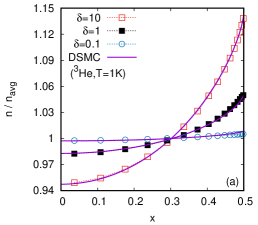
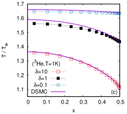
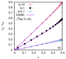
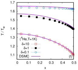
Figure 2: Comparison between the LB (dotted lines and points) and DSMC (continuous lines) results for the profiles of $n$ (left), $u_{y}$ (middle) and $T$ (right) through half of the channel ($0\leq x\leq L/2$), for ${}^{3}{\rm He}$ (top) and ${}^{4}{\rm He}$ (bottom) gas constituents. The wall temperature is set to $T_{w}=1\ {\rm K}$ and the wall velocity is $u_{w}=\sqrt{2K_{B}T_{w}/m}$.

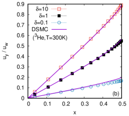
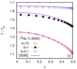
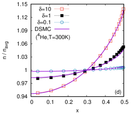
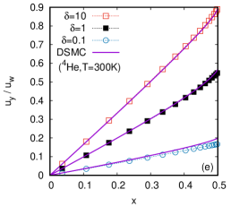
Figure 3: The same as in Fig. 2, but with wall temperature $T_{w}=300\ {\rm K}$.

Figures 2 and 3 show a comparison of the LB and DSMC results for $T_{w}=1\ {\rm K}$ and $300\ {\rm K}$ at the level of the profiles of $n$, $u_{y}$ and $T$, for both the ${}^{3}{\rm He}$ and the ${}^{4}{\rm He}$ gases. Good agreement can be seen at $\delta=10$, while at $\delta=0.1$, there are some discrepancies between the results for $u_{y}$ and $T$. The discrepancy in the temperature profile persists also at $\delta=1$.

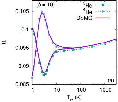
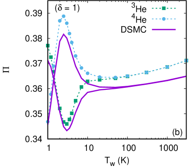
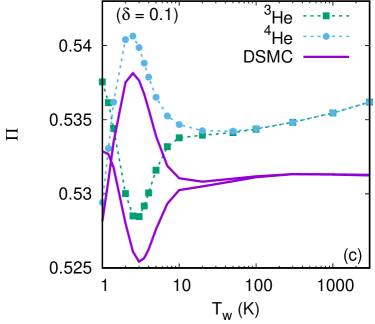
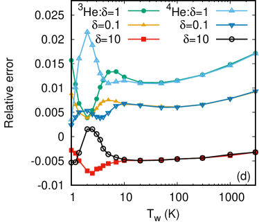
Figure 4: (a-c) Dependence of $\Pi$ (37) on the wall temperature $T_{w}$ for both ${}^{3}{\rm He}$ and ${}^{4}{\rm He}$, at $\delta=10$, $1$ and $0.1$. (d) Relative error $\Pi_{\rm LB}/\Pi_{\rm DSMC}-1$ as a function of $T_{w}$ for $\delta\in\{10,1,0.1\}$.

We next consider a comparison of the LB and DSMC results for the off-diagonal component of the stress tensor $T_{xy}$, which we present through the non-dimensional number

$$\Pi=-\frac{T_{xy}v_{\rm ref}}{P_{\rm ref}u_{w}\sqrt{2}}.$$ (37)

Noting that $u_{w}=\sqrt{2K_{B}T_{w}/m}=v_{\rm ref}\sqrt{2}$, it can be seen that $\Pi=-T_{xy}/2P_{\rm ref}$. Figures 4(a-c) compare the LB and DSMC results for $\Pi$ with respect to $T_{w}$ for $1\ {\rm K}\leq T_{w}\leq 3000\ {\rm K}$, at $\delta=10$, $1$ and $0.1$. It can be seen that $\Pi$ presents only slight variations with respect to $T_{w}$ at fixed values of $\delta$ and the LB results generally follow the same trend as the DSMC results. The general shape of these variations are similar to those of the associated viscosity index $\omega$, shown in Fig. 1(b). The agreement between the LB and DSMC results deteriorates as $\delta$ is decreased, however the relative error $\Pi_{\rm LB}/\Pi_{\rm DSMC}-1$ always remains below $2.5\%$, being largest surprisingly at $\delta\simeq 1$.

The simulation results presented in this section for $\delta=1$ and $10$ were obtained using the models ${\rm HHLB}(6;7)\times{\rm HLB}(6;7)$. As remarked in Refs. ambrus16jcp ; ambrus18pre , higher orders $Q_{x}$ of the half-range Gauss-Hermite quadrature are required when $\delta\lesssim 1$ in order to get accurate solutions of the relaxation time model equation. For this reason, the results presented for $\delta=0.1$ are obtained using the ${\rm HHLB}(10;16)\times{\rm HLB}(6;7)$ model. The values obtained for $\Pi$ (37) using these models were within $0.1\%$ of those obtained with the reference model ${\rm HHLB}(10;50)\times{\rm HLB}(6;7)$ on a grid employing $S=48$ points. Note that also the values of $\Pi$, obtained with the DSMC method, have an error below $0.1\%$ sharipov18 .

V CONCLUSION

In this paper, we presented a comparison of lattice Boltzmann (LB) and direct simulation Monte Carlo (DSMC) results in the context of Couette flow between parallel plates for ${}^{3}{\rm He}$ and ${}^{4}{\rm He}$ gases at temperatures between $1\ {\rm K}$ and $3000\ {\rm K}$. The LB implementation employs the half-range and full-range Gauss-Hermite quadratures on the $x$ and $y$ axes, respectively. The order $Q_{y}=7$ of the full-range Gauss-Hermite quadrature is sufficient to obtain accurate results for all tested values of the rarefaction parameter $\delta$. The quadrature order on the horizontal axis is taken to be $Q_{x}=7$ when $\delta=1$ and $\delta=10$, while at $\delta=0.1$, it is increased to $Q_{x}=16$. The total number of velocities is $2Q_{x}Q_{y}=98$ for $\delta=1$ and $\delta=10$, while at $\delta=0.1$, $224$ velocities are required in order to maintain good accuracy. The agreement obtained with the DSMC results is very good and the relative error in the off-diagonal component $T_{xy}$ of the pressure tensor remains under $2.5\%$, even at $\delta=0.1$. The use of the fifth order WENO scheme and of a third order TVD Runge-Kutta algorithm allows accurate results to be obtained using only $16$ grid nodes on the right half of the channel, which are appropriately stretched towards the diffuse reflecting wall. While the discussion in this paper is limited to the Couette flow between parallel plates, we note that the LB models based on half-range quadratures can be employed also for flows in non-rectangular (curved) domains, e.g., when coupled with the vielbein approach, as discussed in Ref. busuioc19 .

VI ACKNOWLEDGMENTS

V.E.A. was supported by a grant of the Romanian Ministry of Research and Innovation, CCCDI-UEFISCDI, project number PN-III-P1-1.2-PCCDI-2017-0371, within PNCDI III. F.Sh. is supported by CNPq (Brazil), grant 303697/2014-8.

References

- (1) P. L. Bhatnagar, E. P. Gross, M. Krook, Phys. Rev. 94, 511–525 (1954).
- (2) E. M. Shakhov, Fluid Dyn. 3, 95–96 (1968).
- (3) F. Sharipov, Rarefied gas dynamics (Wiley-VCH, 2016).
- (4) Z. Guo, K. Xu, and R. Wang, Phys. Rev. E 88, 033305 (2013).
- (5) A. Xu, G. Zhang, Y. Zhang, “Discrete Boltzmann modeling of compressible flows”, in Kinetic Theory, edited by G. Z. Kyzas and A. C. Mitropoulos (IntechOpen, Washington, DC, 2018), pp. 450–458.
- (6) V. E. Ambru\cbs and V. Sofonea, J. Comput. Phys. 316, 760–788 (2016).
- (7) W. P. Yudistiawan, S. K. Kwak, D. V. Patil, and S. Ansumali, Phys. Rev. E 82, 046701 (2010).
- (8) V. E. Ambru\cbs and V. Sofonea, Phys. Rev. E 86, 016708 (2012).
- (9) J. Meng, Y. Zhang, N. G. Hadjiconstantinou, G. A. Radtke, and X. Shan, J. Fluid Mech. 718, 347–370 (2013).
- (10) B. Piaud, S. Blanco, R. Fournier, V. E. Ambru\cbs and V. Sofonea, Int. J. Mod. Phys. C 25, 1340016 (2014).
- (11) V. E. Ambru\cbs and V. Sofonea, J. Comput. Sci. 17, 403–417 (2016).
- (12) E. P. Gross, E. A. Jackson, and S. Ziering, Ann. Phys. 1, 141–167 (1957).
- (13) S. Takata, H. Funagane, J. Fluid Mech. 717, 30–47 (2013).
- (14) F. Sharipov, Physica A 508, 797–805 (2018).
- (15) W. Cencek, M. Przybytek, J. Komasa, J. B. Mehl, B. Jeziorski, and K. Szalewicz, J. Chem. Phys. 136, 224303 (2012).
- (16) V. E. Ambru\cbs and V. Sofonea, Phys. Rev. E 98, 063311 (2018).
- (17) Z.-H. Li, H.-X. Zhang, J. Comput. Phys. 193, 708–738 (2004).
- (18) J. Meng, L. Wu, J. M. Reese, Y. Zhang, J. Comput. Phys. 251, 383–395 (2013).
- (19) L. Gibelli, Phys. Fluids 24, 022001 (2012).
- (20) F. B. Hildebrand, Introduction to Numerical Analysis, Second edition (Dover Publications, 1987).
- (21) B. Shizgal, Spectral Methods in Chemistry and Physics: Applications to Kinetic Theory and Quantum Mechanics (Scientific Computation) (Springer, 2015).
- (22) C. W. Shu and S. Osher, J. Comput. Phys. 77, 439–471 (1988).
- (23) G. S. Jiang and C. W. Shu, J. Comput. Phys. 126, 202–228 (1996).
- (24) R. Mei and W. Shyy, J. Comput. Phys. 143, 426–448 (1998).
- (25) S. Busuioc and V. E. Ambru\cbs, Phys. Rev. E, in press (arXiv:1708.05944 [physics.flu-dyn]).