Logarithmic-corrected $R^{2}$ Gravity Inflation in the Presence of Kalb-Ramond Fields

Abstract

In this paper we shall study the inflationary aspects of a logarithmic corrected $R^{2}$ Starobinsky inflation model, in the presence of a Kalb-Ramond field in the gravitational action of $F(R)$ gravity. Our main interest is to pin down the effect of this rank two antisymmetric tensor field on the inflationary phenomenology of the $F(R)$ gravity theory at hand. The effects of the Kalb-Ramond field are expected to be strong during the inflationary era, however as the Universe expands, the energy density of the Kalb-Ramond field scales as $\sim a^{-6}$ so dark matter and radiation dominate over the Kalb-Ramond field effects. In general, antisymmetric fields constitute the field content of superstring theories, and thus their effect at the low-energy limit of the theory is expected to be significant. As we will show, for a flat Friedmann-Robertson-Walker metric, the Kalb-Ramond field actually reduces to a scalar field, so it is feasible to calculate the observational indices of inflation. We shall calculate the spectral index and the tensor-to-scalar ratio for the model at hand, by assuming two conditions for the resulting Kalb-Ramond scalar field, the slow-roll and the constant-roll condition. As we shall demonstrate, in both the slow-roll and constant-roll cases, compatibility with the latest observational data can be achieved. Also the effect of the Kalb-Ramond field on the inflationary phenomenology is to increase the amount of the predicted primordial gravitational radiation, in comparison to the corresponding $f(R)$ gravities, however the results are still compatible with the observational data.

1 Introduction

The inflationary paradigm [1, 2, 5, 6, 7, 8] is one of the two most successful scenarios that can consistently describe the primordial era of our Universe, with the second scenario being the bounce cosmology scenario [9]. Both scenarios can predict a nearly scale invariant power spectrum and a small amount of gravitational radiation, which are also verified and tightly constrained by the latest Planck [10] and BICEP2/Keck-Array data [11]. Due to the constraints coming from the observations, the number of viable models of inflation have been narrowed down, and the quest for modern theoretical cosmologists is to find the an optimal description for the primordial era than can produce a nearly scale invariant power spectrum, and a small amount of gravitational radiation, and at the same time describe with the same model the late-time acceleration era. Modified gravity [12, 13, 14, 15, 16, 17] and specifically $F(R)$ gravity, serves as a theoretical framework which can describe successfully both the early and late-time acceleration eras, see for example the model [18] for a characteristic model of this sort. In the context of $F(R)$ gravity, it is possible to generate quite successful models of inflation, with the most well-known being the Starobinsky model [2], see also [3, 4] for a recent modification of the Starobinsky model. In this line of research, studying modifications of the standard $R^{2}$ Starobinsky inflation model, may provide useful insights with regard to both the early-time and the late-time acceleration eras. In view of this aspects, in this work we shall consider a logarithmic-corrected $R^{2}$ model of the form,

$$F(R)=R+\alpha R^{2}+\beta R^{2}\ln{(\beta R)}\,,$$ (1.1)

with $\alpha$, $\beta$ being constant parameters of the model, in the presence of a Kalb-Ramond (KR) field $B_{\mu\nu}$ in the gravitational action of the vacuum $F(R)$ gravity. The logarithmic $F(R)$ gravity model of Eq. (1.1) is known to provide a viable early-time phenomenology and a qualitatively consistent late-time phenomenology [19]. Actually, due to fact that logarithmic corrections are induced by one-loop effects in quantum gravity, there is still much interest to inflationary phenomenology in the context of logarithmic corrected modified gravity, see for example [20, 21, 22, 23, 24, 19, 25]. So in this work we question the viability of the model in the presence of this string theory inspired KR field. The presence of this string-inspired term is motivated by the fact that during the primordial epoch, quantum gravity or string theory effects may have a significant imprint on the evolution of the Universe, so in our case we quantify the quantum epoch’s imprint on the evolution of the Universe, by using this rank two KR antisymmetric tensor field. In general, antisymmetric tensor fields or equivalently $p$-forms, constitute the field content of all superstring models, and in effect these can actually have a realistic impact in the low-energy limit of the theory [26]. In support of this, the Calabi-Yau compactifications of ten dimensional superstring theories to four dimensions, lead to low-energy supergravity theories which contain electric and magnetic fluxes of various $p$-form antisymmetric fields. These theories are intriguing due to the resolution of the vacuum degeneracy that the resulting scalar potentials provide. In fact, the magnetic charges of the low-energy supergravity theory generate mass terms for the $p$-forms, so in effect one obtains supersymmetric models which contain antisymmetric tensor fields [26]. In this work we shall consider the effect of a massless antisymmetric KR field on $F(R)$ gravity inflation, and the effects of a massive antisymmetric field will be studied in a future work. For a relevant work on the effect of KR fields in $F(R)$ gravity, see [27].

As the Universe evolves and cools down, the contribution of the KR field on the evolutionary process reduces significantly, and at present day it does not affect the Universe’s evolution at all. Therefore, in this work we shall consider the effects of this string inspired KR field on the observational indices of inflation, and specifically on the spectral index of the primordial curvature perturbations and on the tensor-to-scalar ratio. On the other hand, the motivation for using a logarithmic corrected $R^{2}$ Starobinsky inflation, comes from studies which include one-loop corrections in higher derivative quantum gravity [24]. Thus the main focus in this work is to confront phenomenologically the logarithmic-corrected $R^{2}$ Starobinsky inflation model in the presence of a KR field, with the observational data coming from the Planck [10] and the BICEP2/Keck-Array collaborations [11]. For the calculation, we shall consider the slow-roll and constant-roll [28, 29, 30, 31, 32, 33, 34, 35, 36, 37, 38, 39, 40, 41, 42, 43, 44, 45, 46, 47, 48, 49, 50, 51, 52, 53, 54, 55, 56, 57, 58, 59] evolution cases. As we shall demonstrate, in both cases the resulting inflationary phenomenology can be compatible with the observational data, by appropriately choosing the free parameters of the gravitational model at hand.

The paper is organized as follows: In section II, we briefly discuss how a general $F(R)$ gravity model can be recast into Einstein gravity plus a scalar field. In section III we introduce the KR $F(R)$ gravity model, present the cosmological equations of motion for a flat Friedmann-Robertson-Walker (FRW) metric and we present the form of the gravitational equations under the assumptions of having a constant-roll and a slow-roll condition imposed on the evolution of the KR field. In section IV the phenomenological aspects of the model are studied in detail, and finally the conclusions follow at the end of the paper.

2 $F(R)$ Gravity in the Einstein Frame

In this section, we briefly discuss how the higher curvature $F(R)$ gravity model in four dimensions can be recast into an Einstein gravity theory with a scalar field. The Jordan frame vacuum $F(R)$ action has the following form,

$$S=\int d^{4}x\sqrt{-g}\Big{(}\frac{F(R)}{2\kappa^{2}}\Big{)}\,,$$ (2.1)

where $g$ is the determinant of the metric $g_{\mu\nu}$, $R$ denotes the Ricci scalar and finally $\frac{1}{2\kappa^{2}}=M_{p}^{2}$ where $M_{p}$ is the Planck mass. Introducing an auxiliary field $A$, the gravitational action (2.1), the latter can equivalently be cast as follows,

$$S=\int d^{4}x\sqrt{-g}\frac{1}{2\kappa^{2}}\Big{(}F^{\prime}(A)(R-A)+F(A)\Big{)}\,,$$ (2.2)

Upon varying the gravitational action with respect to the auxiliary field $A$, one easily obtains the solution $A=R$. Plugging back this solution $A=R$ into the action (2.2), the original action of Eq. (2.1) can be reproduced. At this stage, we perform the following conformal transformation of the metric ($g_{\mu\nu}(x)$),

$$g_{\mu\nu}(x)\longrightarrow\widetilde{g}_{\mu\nu}(x)=e^{-\sqrt{\frac{2}{3}}\kappa\xi}g_{\mu\nu}(x)$$ (2.3)

where $\xi(x)$ is the conformal factor and it is related to the auxiliary field in the following way $F^{\prime}(A)=e^{-[\sqrt{\frac{2}{3}}\kappa\xi]}$. If $R$ and $\tilde{R}$ are the Ricci scalars corresponding to the metrics $g_{\mu\nu}$ and $\tilde{g}_{\mu\nu}$ respectively, then these are related as follows,

$$R=e^{-\Big{(}\sqrt{\frac{2}{3}}\kappa\xi\Big{)}}\Big{(}\tilde{R}-\kappa^{2}\tilde{g}^{\mu\nu}\partial_{\mu}\xi\partial_{\nu}\xi+2\kappa\sqrt{\frac{3}{2}}\tilde{\Box}\xi\Big{)}\,.$$

where $\tilde{\Box}$ represents the d’ Alembertian operator formed by the metric tensor $\tilde{g}_{\mu\nu}$. Due to the above relation between $R$ and $\tilde{R}$, the action (2.2) can be written as follows,

$$S=\int d^{4}x\sqrt{-\tilde{g}} \bigg{[} \frac{1}{2\kappa^{2}}e^{[\sqrt{\frac{2}{3}}\kappa\xi]}F^{\prime}(A)\bigg{(}\tilde{R}-\kappa^{2}\tilde{g}^{\mu\nu}\partial_{\mu}\xi\partial_{\nu}\xi+2\kappa\sqrt{\frac{3}{2}}\tilde{\Box}\xi\bigg{)}$$ (2.4)

$$- \frac{1}{2\kappa^{2}}e^{2[\sqrt{\frac{2}{3}}\kappa\xi]}\bigg{(}AF^{\prime}(A)-F(A)\bigg{)}\bigg{]}$$

Considering $F^{\prime}(A)>0$ and using the aforementioned relation between $\xi$ and $F^{\prime}(A)$, one obtains the following scalar-tensor action,

$$S = \int d^{4}x\sqrt{-\tilde{g}}\bigg{[}\frac{\widetilde{R}}{2\kappa^{2}}-\frac{1}{2}\tilde{g}^{\mu\nu}\partial_{\mu}\xi\partial_{\nu}\xi-\bigg{(}\frac{AF^{\prime}(A)-F(A)}{2\kappa^{2}F^{\prime}(A)^{2}}\bigg{)}\bigg{]}$$ (2.5)

Noticeably the field $\xi(x)$ acts as a scalar field with a potential $V(A(\xi))=\frac{AF^{\prime}(A)-F(A)}{2\kappa^{2}F^{\prime}(A)^{2}}$. Thus the higher curvature degree of freedom in the Jordan frame, after a conformal transformation manifests itself in terms of the scalar field degree of freedom $\xi(x)$ with a potential $V(\xi)$, which in turn depends on the functional form of $F(R)$. Further it is also important to note that for $F^{\prime}(R)<0$, the kinetic term of the scalar field $\xi$, as well as the Ricci scalar $R$ in the above action come with wrong sign, which indicates the existence of a ghost field. Thus to avoid the ghost like structures, the derivative of the functional form of the $F(R)$ gravity, namely $F^{\prime}(R)$ must be greater than zero. Later we shall show that in the model we shall study, this condition is indeed satisfied.

3 The Logarithmic $F(R)$ Gravity Model in the Presence of the Kalb-Ramond Field

In this section we shall present the logarithmic-corrected $F(R)$ gravity model, in the presence of a KR field and we also employ the formalism for the case of a flat cosmological evolution. The vacuum gravitational action of the model is,

$$S = \int d^{4}x\sqrt{-g}\bigg{[}\frac{F(R)}{2\kappa^{2}}-\frac{1}{12}H_{\mu\nu\rho}H^{\mu\nu\rho}\bigg{]}$$ (3.1)

$$= \int d^{4}x\sqrt{-g}\bigg{[}\frac{1}{2\kappa^{2}}\bigg{(}R+\alpha R^{2}+\beta R^{2}\ln{(\beta R)}\bigg{)}-\frac{1}{12}H_{\mu\nu\rho}H^{\mu\nu\rho}\bigg{]}$$

where $\frac{1}{2\kappa^{2}}=M_{p}^{2}$. Moreover $H_{\mu\nu\alpha}$ is the field strength tensor of the KR field, defined by $H_{\mu\nu\alpha}=\partial_{[\mu}B_{\nu\alpha]}$. The field strength tensor $H_{\mu\nu\alpha}$ is invariant under the KR gauge transformation, $B_{\mu\nu}\rightarrow B_{\mu\nu}+\partial_{\mu}\omega_{\nu}-\partial_{\nu}\omega_{\mu}$ and consequently, the action (3.1) is also invariant under this gauge transformation. However the form of $F(R)$ gravity clearly indicates that in the regime of $\alpha$, $\beta$ $>0$, $F^{\prime}(R)$ comes with positive sign (for $R>0$) which in turn renders the model ghost-free. Thus in the rest of this work we shall consider only positive values for the parameters $\alpha$ and $\beta$. By using the formalism of the previous section we can rewrite the action (3.1) into a scalar-tensor form,

$$S = \int d^{4}x\sqrt{-\tilde{g}}\bigg{[}\frac{\widetilde{R}}{2\kappa^{2}}-\frac{1}{2}\tilde{g}^{\mu\nu}\partial_{\mu}\xi\partial_{\nu}\xi-V(\xi)$$ (3.2)

$$- \frac{1}{12}e^{-\sqrt{\frac{2}{3}}\kappa\xi}H_{\mu\nu\rho}H_{\alpha\beta\delta}\tilde{g}^{\mu\alpha}\tilde{g}^{\nu\beta}\tilde{g}^{\rho\delta}\bigg{]}\,,$$

with the scalar field being related to the higher curvature degrees of freedom as follows,

$$\sqrt{\frac{2}{3}}\kappa\xi(R)=\ln{\bigg{[}\frac{1}{1+(2\alpha+\beta)R+2\beta R\ln{(\beta R)}}\bigg{]}}\,,$$ (3.3)

and the scalar potential $V(\xi)$ has the following form,

$$V(\xi(R))=\frac{1}{2\kappa^{2}}\bigg{[}\frac{\big{[}(\alpha+\beta)R^{2}+\beta R^{2}\ln{(\beta R)}\big{]}}{\big{[}1+(2\alpha+\beta)R+2\beta R\ln{(\beta R)}\big{]}^{2}}\bigg{]}\,,$$ (3.4)

and finally with $\xi=\xi(R)$ being given in Eq. (3.3). We need to note that the transformations of the KR field between Jordan and Einstein frames has been worked out for general $f(R)$ gravity theories in Ref. [27]. The potential has a minimum value at,

$$2\alpha+3\beta+2\beta\ln{(\beta<R>_{min})}=0\,,$$ (3.5)

and a maximum value which is,

$$<R>_{max}=1/\beta\,.$$ (3.6)

Moreover at the large curvature regime $R\gg 1$, $V(R)$ behaves as $\frac{1}{8\kappa^{2}\beta\ln{(\beta R)}}$ and it thus slowly approaches the value zero as $R\rightarrow\infty$. Furthermore, from Eq. (3.4), one obtains the first and second derivative of the potential, which are,

$$\frac{dV}{d\xi} = \frac{dV}{dR}\frac{dR}{d\xi}$$ (3.7)

$$= \frac{\sqrt{\frac{2}{3}}}{2\kappa}\bigg{[}\frac{(-R+\beta R^{2})}{[1+(2\alpha+\beta)R+2\beta R\ln{(\beta R)}]^{2}}\bigg{]}$$

and

$$\frac{d^{2}V}{d\xi^{2}}=\frac{1}{3}\bigg{[}\frac{-3R-2\alpha R^{2}+\beta R^{2}-2\beta R^{2}\ln{(\beta R)}}{[1+(2\alpha+\beta)R+2\beta R\ln{(\beta R)}]^{2}}+\frac{1}{2\alpha+3\beta+2\beta\ln{(\beta R)}}\bigg{]}\,,$$ (3.8)

which we will need later on in order to determine the spectral index and tensor-to-scalar ratio. However it is evident from Eq. (3.2) that due to the presence of the scalar field $\xi(x)$ (from higher curvature degrees of freedom), the kinetic term of the KR field becomes non-canonical. In order to make it canonical, we redefine the field as follows,

$$B_{\mu\nu}\longrightarrow\widetilde{B}_{\mu\nu}=e^{-\frac{1}{2}\sqrt{\frac{2}{3}}\kappa\xi}B_{\mu\nu}\,.$$ (3.9)

In terms of the redefined field, the final form of the scalar-tensor action is the following,

$$S=\int d^{4}x\sqrt{-\tilde{g}}\bigg{[}\frac{\widetilde{R}}{2\kappa^{2}}-\frac{1}{2}\tilde{g}^{\mu\nu}\partial_{\mu}\xi\partial_{\nu}\xi-V(\xi)-\frac{1}{12}\tilde{H}_{\mu\nu\rho}\tilde{H}^{\mu\nu\rho}\bigg{]}\,,$$ (3.10)

and we shall consider the case where $\kappa\tilde{B}_{\mu\nu}<1$, and also $V(\xi)$ is given in Eq. (3.4). Accordingly, we shall determine the cosmological field equations for the scalar-tensor model, from which one can go back to the original $F(R)$ gravity model of Eq. (3.1) by using an inverse conformal transformation.

3.1 Cosmological Field Equations for the Scalar-tensor Model

In order to obtain the field equations of the scalar-tensor (ST) action (3.10), first we determine the energy-momentum tensor for $\xi(x)$ and $\tilde{B}_{\mu\nu}(x)$, which are,

$$T_{\mu\nu}[\xi] = \frac{2}{\sqrt{-\tilde{g}}}\frac{\delta}{\delta\tilde{g}^{\mu\nu}}\bigg{[}\sqrt{-\tilde{g}}\bigg{(}\frac{1}{2}\tilde{g}^{\alpha\beta}\partial_{\alpha}\xi\partial_{\beta}\xi+V(\xi)\bigg{)}\bigg{]}$$ (3.11)

$$= \partial_{\mu}\xi\partial_{\nu}\xi-\tilde{g}_{\mu\nu}\bigg{(}\frac{1}{2}\tilde{g}^{\alpha\beta}\partial_{\alpha}\xi\partial_{\beta}\xi+V(\xi)\bigg{)}$$

and

$$T_{\mu\nu}[\tilde{B}] = \frac{2}{\sqrt{-\tilde{g}}}\frac{\delta}{\delta\tilde{g}^{\mu\nu}}\bigg{[}\frac{1}{12}\sqrt{-\tilde{g}}\tilde{g}^{\mu\alpha}\tilde{g}^{\nu\beta}\tilde{g}^{\lambda\gamma}\tilde{H}_{\mu\nu\lambda}\tilde{H}_{\alpha\beta\gamma}\bigg{]}$$ (3.12)

$$= \frac{1}{6}\bigg{[}3\tilde{g}_{\nu\rho}\tilde{H}_{\alpha\beta\mu}\tilde{H}^{\alpha\beta\rho}-\frac{1}{2}\tilde{g}_{\mu\nu}\tilde{H}_{\alpha\beta\gamma}\tilde{H}^{\alpha\beta\gamma}\bigg{]}$$

respectively. Our motivation is to investigate whether the $F(R)$ model that we chose in the present context can be considered as a viable inflationary model, in view of the observational constraints of $Planck$ 2018 and of the BICEP2 Keck-Array data. We shall consider a flat FRW metric of the form,

$$\tilde{ds}^{2}=-dt^{2}+a^{2}(t)\big{[}dx^{2}+dy^{2}+dz^{2}\big{]}$$ (3.13)

where $t$ and $a(t)$ are cosmic time and scale factor respectively. However before presenting the field equations, we want to emphasize that due to antisymmetric nature of the KR field, the tensor $\tilde{H}_{\mu\nu\lambda}$ has four independent components in the context of four dimensional spacetime, which can be expressed as follows,

$$\tilde{H}_{012}=h_{1},\,\,\,\,\tilde{H}^{012}=h^{1}\,,$$

$$\tilde{H}_{013}=h_{2},\,\,\,\,\tilde{H}^{013}=h^{2}\,,$$

$$\tilde{H}_{023}=h_{3},\,\,\,\,\tilde{H}^{023}=h^{3}\,,$$

$$\tilde{H}_{123}=h_{4},\,\,\,\,\tilde{H}^{123}=h^{4}\,,$$ (3.14)

At this stage, it is worth mentioning that due to the presence of the four independent components, the KR field tensor $\tilde{H}_{\mu\nu\alpha}$ can be equivalently expressed by a vector field (which has also four independent components in four dimensions) [60] as $\tilde{H}_{\mu\nu\alpha}=\varepsilon_{\mu\nu\alpha\beta}\Upsilon^{\beta}$, with $\Upsilon^{\beta}$ being the vector field. Therefore, Eq. (3.14) for the FRW metric can yield the components of the energy momentum tensors $T_{\mu\nu}[\xi]$ and $T_{\mu\nu}[\tilde{B}]$, which are,

$$T_{00}[\xi] = \frac{1}{2}\dot{\xi}^{2}+V(\xi)$$

$$T_{11}[\xi] = T_{22}[\xi]=T_{33}[\xi]=a(t)^{2}\bigg{[}\frac{1}{2}\dot{\xi}^{2}-V(\xi)\bigg{]}$$

and

$$T_{00}[\tilde{B}] = \frac{1}{2}\bigg{[}-h_{1}h^{1}-h_{2}h^{2}-h_{3}h^{3}+h_{4}h^{4}\bigg{]}$$

$$T_{11}[\tilde{B}] = \frac{1}{2}a(t)^{2}\bigg{[}h_{1}h^{1}+h_{2}h^{2}-h_{3}h^{3}+h_{4}h^{4}\bigg{]}$$

$$T_{22}[\tilde{B}] = \frac{1}{2}a(t)^{2}\bigg{[}h_{1}h^{1}-h_{2}h^{2}+h_{3}h^{3}+h_{4}h^{4}\bigg{]}$$

$$T_{33}[\tilde{B}] = \frac{1}{2}a(t)^{2}\bigg{[}-h_{1}h^{1}+h_{2}h^{2}+h_{3}h^{3}+h_{4}h^{4}\bigg{]}$$

$$T_{10}[\tilde{B}] = -h_{4}h^{3},\,\,\,\,T_{20}[\tilde{B}]=h_{4}h^{2}$$

$$T_{30}[\tilde{B}] = -h_{4}h^{1},\,\,\,\,T_{12}[\tilde{B}]=a(t)^{2}h_{2}h^{3}$$

$$T_{13}[\tilde{B}] = -a(t)^{2}h_{1}h^{3},\,\,\,\,T_{23}[\tilde{B}]=a(t)^{2}h_{1}h^{2}$$

where the fields are taken to be homogeneous in space. In effect, the off-diagonal Friedmann equations read,

$$h_{4}h^{3}=h_{4}h^{2}=h_{4}h^{1}=h_{2}h^{3}=h_{1}h^{3}=h_{1}h^{2}=0\,,$$ (3.15)

which have the following solution,

$$h_{1}=h_{2}=h_{3}=0,\,\,\,\,h_{4}\neq 0\,.$$ (3.16)

Using this solution, one easily obtains the total energy density and pressure for the matter fields ($\xi$, $\tilde{B}_{\mu\nu}$) which are,

$$\rho_{T}=\bigg{[}\frac{1}{2}\dot{\xi}^{2}+V(\xi)+\frac{1}{2}h_{4}h^{4}\bigg{]}\,,$$ (3.17)

$$p_{T}=\bigg{[}\frac{1}{2}\dot{\xi}^{2}-V(\xi)+\frac{1}{2}h_{4}h^{4}\bigg{]}\,,$$

with the “dot” denoting differentiation with respect to the cosmic time. In effect, the diagonal Friedmann equations turn out to be,

$$H^{2}=\frac{\kappa^{2}}{3}\bigg{[}\frac{1}{2}\dot{\xi}^{2}+V(\xi)+\frac{1}{2}h_{4}h^{4}\bigg{]}\,,$$ (3.18)

and

$$2\dot{H}+3H^{2}+\kappa^{2}\bigg{[}\frac{1}{2}\dot{\xi}^{2}-V(\xi)+\frac{1}{2}h_{4}h^{4}\bigg{]}=0\,,$$ (3.19)

where $H=\frac{\dot{a}}{a}$ denotes the Hubble parameter of the scalar-tensor model. Furthermore, the field equations for the KR field ($\tilde{B}_{\mu\nu}$) and the scalar field ($\xi$) are given by,

$$\tilde{\nabla}_{\mu}\tilde{H}^{\mu\nu\lambda}=\frac{1}{a^{3}(t)}\partial_{\mu}\bigg{[}a^{3}(t)\tilde{H}^{\mu\nu\lambda}\bigg{]}=0\,,$$ (3.20)

and

$$\ddot{\xi}+3H\dot{\xi}+\frac{\partial V}{\partial\xi}=0\,,$$ (3.21)

respectively. However, first we investigate Eq. (3.20). As we will see shortly, the only information that can be obtained from Eq. (3.20) is that the non-zero component of $\tilde{H}_{\mu\nu\alpha}$ (i.e $\tilde{H}_{123}=h_{4}$) depends solely on the cosmic time $t$. This can easily by seen, by expanding Eq. (3.20) as follows,

$$\partial_{0} \bigg{[}a^{3}(t)\tilde{H}^{0\nu\lambda}\bigg{]}+\partial_{1}\bigg{[}a^{3}(t)\tilde{H}^{1\nu\lambda}\bigg{]}$$ (3.22)

$$+\partial_{2} \bigg{[}a^{3}(t)\tilde{H}^{2\nu\lambda}\bigg{]}+\partial_{3}\bigg{[}a^{3}(t)\tilde{H}^{3\nu\lambda}\bigg{]}=0\,.$$

Therefore for,

• $\nu=2$ and $\lambda=3$, Eq. (3.22) becomes

  $$\partial_{t} \bigg{[}a^{3}(t)\tilde{H}^{023}\bigg{]}+\partial_{x}\bigg{[}a^{3}(t)\tilde{H}^{123}\bigg{]}$$ (3.23)

  $$+\partial_{y} \bigg{[}a^{3}(t)\tilde{H}^{223}\bigg{]}+\partial_{z}\bigg{[}a^{3}(t)\tilde{H}^{323}\bigg{]}=0$$

  Due to the antisymmetric nature of the KR field, the last two terms of the above equation vanish identically. Furthermore, from Eq. (3.16), we get $\tilde{H}^{023}=0$. As a result, only the second term of Eq. (3.23) survives, from which we may conclude that the non-zero component of the KR field ($\tilde{H}^{123}$) is independent of the spatial coordinates $x$ i.e. $\partial_{x}\bigg{[}\tilde{H}^{123}\bigg{]}=0$.

• For $\nu=1$ and $\lambda=3$, Eq. (3.22) becomes,

  $$\partial_{t} \bigg{[}a^{3}(t)\tilde{H}^{013}\bigg{]}+\partial_{x}\bigg{[}a^{3}(t)\tilde{H}^{113}\bigg{]}$$ (3.24)

  $$+\partial_{y} \bigg{[}a^{3}(t)\tilde{H}^{213}\bigg{]}+\partial_{z}\bigg{[}a^{3}(t)\tilde{H}^{313}\bigg{]}=0$$

  Here the third term survives, which ensures that $\tilde{H}^{123}$ is independent of $y$.

• For $\nu=1$ and $\lambda=2$, Eq. (3.22) becomes,

  $$\partial_{t} \bigg{[}a^{3}(t)\tilde{H}^{012}\bigg{]}+\partial_{x}\bigg{[}a^{3}(t)\tilde{H}^{112}\bigg{]}$$ (3.25)

  $$+\partial_{y} \bigg{[}a^{3}(t)\tilde{H}^{212}\bigg{]}+\partial_{z}\bigg{[}a^{3}(t)\tilde{H}^{312}\bigg{]}=0$$

  where the fourth term gives $\partial_{z}\bigg{[}\tilde{H}^{123}\bigg{]}=0$.

Therefore, it is clear that the non-zero component of the KR field i.e $\tilde{H}^{123}$ depends solely on the cosmic time coordinate, which is also expected from the gravitational field equations. In view of these results, now we turn our focus to the other field equations. Differentiating both sides (with respect to $t$) of Eq. (3.18), we get,

$$6H\dot{H}=\kappa^{2}\bigg{[}\dot{\xi}\ddot{\xi}+V^{\prime}(\xi)\dot{\xi}+\frac{1}{2}\frac{d}{dt}(h_{4}h^{4})\bigg{]}$$

Furthermore, Eqs. (3.18) and (3.19) lead to the expression as $2\dot{H}=-\kappa^{2}\big{[}\dot{\xi}^{2}+h_{4}h^{4}\big{]}$. Plugging back this expression of $\dot{H}$ into the above equation and using the scalar field equation of motion, we obtain the following cosmic evolution of $h_{4}h^{4}$,

$$\frac{d}{dt}(h_{4}h^{4})=-6Hh_{4}h^{4}$$ (3.26)

Recall that the term $\frac{1}{2}h_{4}h^{4}$ represents the energy density $\tilde{\rho}_{KR}$ corresponding to the KR field. Therefore Eq. (3.26) can be alternatively written as follows,

$$\frac{d\tilde{\rho}_{KR}}{dt}=-6H\tilde{\rho}_{KR}\,,$$ (3.27)

$$\tilde{\rho}_{KR}=\frac{h_{0}}{2a^{6}}\,,$$ (3.28)

with $h_{0}$ being an integration constant which must take only positive values in order to get a real valued solution for $h^{4}(t)$. In addition, Eq. (3.28) clearly indicates that the energy density of the KR field ($\tilde{\rho}_{KR}$) is proportional to $1/a^{6}$ and in effect, $\tilde{\rho}_{KR}$ decreases as the Universe expands, in a faster rate in comparison to matter ($\propto 1/a^{3}$) and radiation ($\propto 1/a^{4}$) energy density respectively. With the solution of $h_{4}h^{4}$ at hand (in terms of scale factor, see Eq. (3.28)), there remain two independent equations which are the following,

$$H^{2}=\frac{\kappa^{2}}{3}\bigg{[}\frac{1}{2}\dot{\xi}^{2}+V(\xi)+\frac{1}{2}\frac{h_{0}}{a^{6}}\bigg{]}\,,$$ (3.29)

and

$$\ddot{\xi}+3H\dot{\xi}+\frac{\partial V}{\partial\xi}=0\,.$$ (3.30)

Here, we need to mention that Eqs. (3.29), (3.30) match with the field equations when $\tilde{H}_{\mu\nu\alpha}$ is expressed by using it’s vector representation i.e. $\tilde{H}_{\mu\nu\alpha}=\varepsilon_{\mu\nu\alpha\beta}\Upsilon^{\beta}$. In the Appendix we provide the details of this equivalence between the two field equations. This confirms the equivalence between the two representations (when $\tilde{H}_{\mu\nu\alpha}$ is not represented by a vector field) at the level of equations of motion, which is also in agreement with Ref. [60]. Since we are interested in finding the observational indices of inflation, and specifically the spectral index and the tensor-to-scalar ratio, we shall make some simplifications on the evolution of the KR, field, and specifically we shall assume that it obeys the slow-roll or the constant-roll condition.

Let us first consider the slow-roll case, in which case the assumption which is made is the following,

$$V(\xi)\gg\frac{1}{2}\dot{\xi}^{2}$$ (3.31)

Under these conditions, the field equations become,

$$H^{2}=\frac{\kappa^{2}}{3}\bigg{[}V(\xi)+\frac{h_{0}}{2a^{6}}\bigg{]}~{}~{}~{}~{},$$ (3.32)

$$2\dot{H}+3H^{2}+\kappa^{2}\big{[}-V(\xi)+\frac{h_{0}}{2a^{6}}\big{]}\,,$$ (3.33)

and

$$3H\dot{\xi}+\frac{\partial V}{\partial\xi}=0\,.$$ (3.34)

Therefore from the Einstein’s equations, one obtains $\dot{H}=-\frac{\kappa^{2}h_{0}}{2a^{6}}$, which will be used later on. On the other hand, the constant-roll condition is materialized by the following condition,

$$\frac{\ddot{\xi}}{H\dot{\xi}}=\gamma\,,$$ (3.35)

where $\gamma$ is a real parameter. Such a framework interpolates between the slow-roll inflation, for which $\ddot{\xi}\simeq 0$ and the ultra-slow-roll inflation, satisfying $V^{\prime}(\xi)=0$ over a range of field values. These two regimes are respectively reproduced by $\gamma\simeq 0$ and $\gamma=-3$. However integrating Eq. (3.35) yields the following expression for the velocity of the scalar field (in terms of the scale factor) $\dot{\xi}=Aa^{\gamma}$ ($A$ be the integration constant) [33]. With these expressions of $\dot{\xi}$ and $\ddot{\xi}$, the field equations take the following form,

$$H^{2}=\frac{\kappa^{2}}{3}\bigg{[}\frac{A^{2}}{2}a^{2\gamma}+V(\xi)+\frac{h_{0}}{2a^{6}}\bigg{]}\,,$$ (3.36)

$$2\dot{H}+3H^{2}+\kappa^{2}\bigg{[}\frac{A^{2}}{2}a^{2\gamma}-V(\xi)+\frac{h_{0}}{2a^{6}}\bigg{]}\,,$$ (3.37)

and

$$\big{(}\gamma+3\big{)}H\dot{\xi}+\frac{\partial V}{\partial\xi}=0\,.$$ (3.38)

It may be observed that when $\gamma$ and $A$ tend to zero, the constant-roll field equations match with those corresponding to the slow-roll approximation. However using Eqs. (3.36) and (3.37), we get $\dot{H}=-\frac{\kappa^{2}A^{2}}{2}a^{2\gamma}-\frac{\kappa^{2}h_{0}}{2a^{6}}$, thereby it is clear that the presence of the constant $A$ changes the rate of Hubble parameter in comparison to the slow-roll approximation case, where $\dot{H}=-\frac{\kappa^{2}h_{0}}{2a^{6}}$. Now a major question to address is at the level of a background FRW evolution, and in the context of a linear perturbation theory, how is the massless KR field distinguished from the massless scalar field. We address this issue in detail in the following subsection.

3.2 Perturbation Equations of the KR Theory

The second rank antisymmetric Kalb-Ramond field in $D$-spacetime dimensions has a total of $D(D-1)/2$ independent components, but due to the fact that the time derivatives of only the spatial components of the Kalb-Ramond field appear in the Lagrangian, and in addition the transformation $B_{\mu\nu}\rightarrow B_{\mu\nu}+\partial_{[\mu}\omega_{\nu]}$ leaves the KR field Lagrangian invariant and in conjunction with the fact that a change of the gauge field by $\omega_{\mu}\rightarrow\omega_{\mu}+\partial_{\mu}\varphi$ keeps the gauge transformation unchanged, the actual number of degrees of freedom of a $D$-dimensional KR field is given by $\frac{(D-1)(D-4)}{2}+1$ [61].

Thereby in four dimensions, the KR field has a single degree of freedom which enables one to write down the KR field tensor $H_{\mu\nu\rho}$ in terms of a massless scalar field ($Z$) such that, $H_{\mu\nu\rho}=\epsilon_{\mu\nu\rho\sigma}\partial^{\sigma}Z$, with $\epsilon_{\mu\nu\rho\sigma}=\sqrt{-g}[\mu\nu\rho\sigma]$.
Now we are going to investigate whether the perturbed up to first order cosmological field equations are equivalent when $H_{\mu\nu\rho}$ is represented or not represented by a massless scalar field. This investigation is important as we will use this equivalence in order to determine the slow-roll indices in the next section. Recall that, the background spacetime is described by a spatially homogeneous and isotropic FRW metric given in Eq. (3.13). For this metric, the background field equations, when the KR field tensor is not represented by a massless scalar field, are given in Eqs. (3.18)-(3.21).

3.2.1 The Case of a Massless Scalar Field

The action with a massless scalar field denoted as $Z$, instead of the Kalb-Ramond field, is given by,

$$S=\int d^{4}x\sqrt{-\tilde{g}}\bigg{[}\frac{\tilde{R}}{2\kappa^{2}}-\frac{1}{2}\tilde{g}^{\mu\nu}\partial_{\mu}\xi\partial_{\nu}\xi-V(\xi)-\frac{1}{2}\tilde{g}^{\mu\nu}\partial_{\mu}Z\partial_{\nu}Z\bigg{]}$$ (3.39)

where $\xi$ is the scalar field which arises from higher curvature degrees of freedom. The action leads to the following background Friedmann equations,

$$H^{2}=\frac{\kappa^{2}}{3}\bigg{[}\frac{1}{2}\dot{\xi}^{2}+V(\xi)+\frac{1}{2}\dot{Z}^{2}\bigg{]}$$

$$2\dot{H}+3H^{2}+\kappa^{2}\bigg{[}\frac{1}{2}\dot{\xi}^{2}+V(\xi)+\frac{1}{2}\dot{Z}^{2}\bigg{]}$$ (3.40)

where we made the assumption that $Z$ is spatially homogeneous. Moreover the field equations for $\xi(t)$ and $Z(t)$ are,

$$\ddot{\xi}+3H\dot{\xi}+\frac{\partial V}{\partial\xi}=0$$ (3.41)

and

$$\ddot{Z}+3H\dot{Z}=0$$ (3.42)

respectively. It can be shown that the background field equations (3.40-3.42) match with the field equations (3.18)-(3.21) by making use of the relation $H_{\mu\nu\rho}=\epsilon_{\mu\nu\rho\sigma}\partial^{\sigma}Z$.

The demonstration goes as follows: the aforementioned relation between $H_{\mu\nu\rho}$ and $Z$ immediately leads to the solution $h_{1}=h_{2}=h_{3}=0$ due to the fact that $Z$ is spatially homogeneous. With these solutions, one easily obtains $h_{4}h^{4}=\dot{Z}^{2}$ from which the equivalence between the gravitational field equations (3.40) and (3.18)-(3.21) is established. Finally the expression $h_{4}h^{4}=\dot{Z}^{2}$ also validates the equivalence between the conservation equations for $Z(t)$ and for the KR field respectively.

3.2.2 First Order Perturbed Friedmann Equations

We now consider a perturbed FRW spacetime containing scalar and tensor type perturbations [63]:

$$d\tilde{s}^{2}=-(1+2\alpha)dt^{2}-2a\beta_{,i}dtdx^{i}+a^{2}\bigg{[}\delta_{ij}+2\Psi\delta_{ij}+2\gamma_{,i,j}+2C_{ij}\bigg{]}dx^{i}dx^{j}$$ (3.43)

where $i,j$ denote the spatial indices, $\delta_{ij}$ is the Kronecker symbol and set the background spatial metric. The spacetime dependent variables $\alpha$, $\beta$, $\gamma$, $\Psi$ are the scalar type perturbations while $C_{\alpha\beta}$ is the tensorial one.

3.2.3 With Kalb-Ramond field

In this subsection, we will determine the first order perturbed equations in the presence of a second rank antisymmetric Kalb-Ramond field with the action given by : $S=\int d^{4}x\sqrt{-\tilde{g}}\big{[}\frac{\tilde{R}}{2\kappa^{2}}-\frac{1}{2}\tilde{g}^{\mu\nu}\partial_{\mu}\xi\partial_{\nu}\xi-V(\xi)-\frac{1}{12}\tilde{H}_{\mu\nu\rho}\tilde{H}^{\mu\nu\rho}\big{]}$. However, in view of the perturbations (as shown in Eq.(3.43)), the perturbed components of the energy-momentum tensor are given by the following expressions :

$$\delta T_{0}^{0} = -\bigg{[}\frac{1}{2}h_{4}\delta h^{4}+\frac{1}{2}h^{4}\delta h_{4}+\dot{\xi}\delta\dot{\xi}+V^{\prime}(\xi)\delta\xi\bigg{]}$$

$$\delta T_{i}^{0} = -\bigg{[}h_{4}h^{4}+\dot{\xi}^{2}\bigg{]}v_{,i}$$

$$\delta T_{i}^{j} = \delta^{i}_{j}\bigg{[}\frac{1}{2}h_{4}\delta h^{4}+\frac{1}{2}h^{4}\delta h_{4}+\dot{\xi}\delta\dot{\xi}+V^{\prime}(\xi)\delta\xi\bigg{]}$$ (3.44)

where $\delta h_{4}$ and $\delta\xi$ are the perturbations of KR field and of the scalar field $\xi$ respectively. The above expressions of $\delta T^{\mu}_{\nu}$ along with the introduction $k=3H\alpha-3\dot{\Psi}-\frac{1}{a^{2}}\nabla^{2}\chi$ (where $\nabla$ denotes the Laplacian operator with respect to the background metric) yield the first order perturbed gravitational equations as follows [63],

$$\frac{1}{a^{2}}\nabla^{2}\Psi+Hk=-\frac{\kappa^{2}}{2}\bigg{[}\frac{1}{2}h_{4}\delta h^{4}+\frac{1}{2}h^{4}\delta h_{4}+\dot{\xi}\delta\dot{\xi}+V^{\prime}(\xi)\delta\xi\bigg{]}$$ (3.45)

$$k+\frac{1}{a^{2}}\nabla^{2}\chi=\frac{3}{2}\kappa^{2}a\big{[}h_{4}h^{4}+\dot{\xi}^{2}\big{]}v$$ (3.46)

$$\dot{\chi}+H\chi-\alpha-\Psi=0$$ (3.47)

$$\dot{k}+2Hk+\bigg{(}3\dot{H}+\frac{1}{a^{2}}\nabla^{2}\bigg{)}\alpha=\frac{\kappa^{2}}{2}\bigg{[}2h_{4}\delta h^{4}+2h^{4}\delta h_{4}+4\dot{\xi}\delta\dot{\xi}-2V^{\prime}(\xi)\delta\xi\bigg{]}$$ (3.48)

$$\ddot{C}^{i}_{j}+3H\dot{C}^{i}_{j}-\frac{1}{a^{2}}\nabla^{2}C^{i}_{j}=0$$ (3.49)

where $\chi=a[\beta+a\dot{\gamma}]$. Moreover the perturbed equations for $\xi$ and for the KR field are given by,

$$\delta\ddot{\xi}+3H\delta\dot{\xi}-\frac{1}{a^{2}}\nabla^{2}(\delta\xi)+V^{\prime\prime}(\xi)\delta\xi=\dot{\xi}[k+\dot{\alpha}]+[\ddot{\xi}-V^{\prime}(\xi)]\alpha$$ (3.50)

and

$$\frac{1}{2}\big{[}\dot{h}_{4}\delta\dot{h}^{4}+\dot{h}^{4}\delta\dot{h}_{4}\big{]}+3H\big{[}h_{4}\delta h^{4}+h^{4}\delta h_{4}\big{]}-h_{4}h^{4}\big{[}k+\dot{\alpha}-3H\alpha\big{]}=0$$ (3.51)

respectively, where we consider $\delta h_{1}=\delta h_{2}=\delta h_{3}=\delta h_{4}=0$.
Having presented the perturbed equations in the presence of the KR field, now we turn our focus to the case of a massless scalar field.

3.2.4 With massless scalar field

In this case, the action is given by Eq. (3.39). For such an action, the perturbed components of the energy-momentum tensor take the following form,

$$\delta T_{0}^{0} = -\bigg{[}\dot{Z}\delta\dot{Z}+\dot{\xi}\delta\dot{\xi}+V^{\prime}(\xi)\delta\xi\bigg{]}$$

$$\delta T_{i}^{0} = -\bigg{[}\dot{Z}^{2}+\dot{\xi}^{2}\bigg{]}v_{,i}$$

$$\delta T_{i}^{j} = \delta^{i}_{j}\bigg{[}\dot{Z}\delta\dot{Z}+\dot{\xi}\delta\dot{\xi}+V^{\prime}(\xi)\delta\xi\bigg{]}$$ (3.52)

where $\delta Z$ denotes the perturbation of the massless scalar field $Z$. Combining the above expressions with the previous definitions of $k$ and $\chi$, we get the perturbed gravitational equations,

$$\frac{1}{a^{2}}\nabla^{2}\Psi+Hk=-\frac{\kappa^{2}}{2}\bigg{[}\dot{Z}\delta\dot{Z}+\dot{\xi}\delta\dot{\xi}+V^{\prime}(\xi)\delta\xi\bigg{]}$$ (3.53)

$$k+\frac{1}{a^{2}}\nabla^{2}\chi=\frac{3}{2}\kappa^{2}a\big{[}\dot{Z}^{2}+\dot{\xi}^{2}\big{]}v$$ (3.54)

$$\dot{\chi}+H\chi-\alpha-\Psi=0$$ (3.55)

$$\dot{k}+2Hk+\bigg{(}3\dot{H}+\frac{1}{a^{2}}\nabla^{2}\bigg{)}\alpha=\kappa^{2}\bigg{[}2\dot{Z}\delta\dot{Z}+2\dot{\xi}\delta\dot{\xi}-V^{\prime}(\xi)\delta\xi\bigg{]}$$ (3.56)

$$\ddot{C}^{i}_{j}+3H\dot{C}^{i}_{j}-\frac{1}{a^{2}}\nabla^{2}C^{i}_{j}=0$$ (3.57)

Moreover the perturbed equations for $\xi$ and for $Z$ are given by,

$$\delta\ddot{\xi}+3H\delta\dot{\xi}-\frac{1}{a^{2}}\nabla^{2}(\delta\xi)+V^{\prime\prime}(\xi)\delta\xi=\dot{\xi}[k+\dot{\alpha}]+[\ddot{\xi}-V^{\prime}(\xi)]\alpha$$ (3.58)

and

$$\delta\ddot{Z}+3H\delta\dot{Z}-\dot{Z}(k+\dot{\alpha})-[2\ddot{Z}+3H\dot{Z}]\alpha=0$$ (3.59)

respectively. However the relation $H_{\mu\nu\rho}=\epsilon_{\mu\nu\rho\sigma}\partial^{\sigma}Z$, immediately leads to the following expressions,

$$h_{4}\delta h^{4}=\dot{Z}\delta\dot{Z}-\frac{3}{a}\dot{Z}^{2}\delta a$$

$$h^{4}\delta h_{4}=\dot{Z}\delta\dot{Z}+\frac{3}{a}\dot{Z}^{2}\delta a$$

$$\dot{h}_{4}\delta\dot{h}^{4}+\dot{h}^{4}\delta\dot{h}_{4}=2[\dot{Z}\delta\ddot{Z}+\ddot{Z}\delta\dot{Z}]$$ (3.60)

The above relations transform Eqs. (3.45 - 3.51) to Eqs. (3.53 - 3.59). This validates the equivalence between the set of Eqs. (3.45 - 3.51) and Eqs. (3.53 - 3.59).

Thereby, the first order perturbed cosmological equations are equivalent for the cases when $H_{\mu\nu\alpha}$ is represented by a massless scalar field $Z$. In the present context, as we are interested to determine the spectral index and tensor-to-scalar ratio, we show the equivalence (between KR and massless scalar field) only up to first order perturbed equations and we do not consider the higher order perturbations. However the investigation of such equivalence for second (or higher) order perturbations is important, which we hope to address in a future work.

Having discussed the above issues, we shall calculate the slow-roll indices and the corresponding observational indices for the KR $F(R)$ gravity model at hand. This is the subject of the next section.

4 Inflationary Phenomenology of the Kalb-Ramond $F(R)$ model

Recall that the original higher curvature $F(R)$ model is given by the action given in Eq. (3.1). The spacetime metric for this $F(R)$ model can be extracted from the corresponding scalar-tensor theory (see Eq. (3.13)) with the help of inverse conformal transformation. Thus the line element in $F(R)$ model turns out to be,

$$ds^{2} = e^{\sqrt{\frac{2}{3}}\kappa\xi(t)}\bigg{[}-dt^{2}+a^{2}(t)\big{(}dx^{2}+dy^{2}+dz^{2}\big{)}\bigg{]}$$ (4.1)

$$= -d\tau^{2}+s^{2}(\tau)\big{(}dx^{2}+dy^{2}+dz^{2}\big{)}$$

where $\tau(t)$, $s(\tau)$ are the cosmic time and the scale factor respectively in the $F(R)$ frame and they are defined as follows:

$$\tau(t)=\int dte^{[\frac{1}{2}\sqrt{\frac{2}{3}}\kappa\xi(t)]}\,,$$ (4.2)

and

$$s(\tau(t))=e^{[\frac{1}{2}\sqrt{\frac{2}{3}}\kappa\xi(t)]}a(t)\,.$$ (4.3)

Clearly Eq. (4.2) indicates that $\tau(t)$ is a monotonically increasing function of the cosmic time $t$. Consequently the Hubble parameter ($H_{F}$) in the $F(R)$ frame is defined as $H_{F}=\frac{1}{s(\tau)}\frac{ds}{d\tau}$. Using Eqs. (4.2) and (4.3), we can relate the Hubble parameter to that of the corresponding scalar-tensor model as follows,

$$H_{F}=e^{-\frac{\sqrt{2}\kappa}{2\sqrt{3}}\xi(t)}\bigg{[}H+\frac{\sqrt{2}\kappa}{2\sqrt{3}}\dot{\xi}\bigg{]}\,,$$ (4.4)

where $H$ is the Hubble parameter in the scalar-tensor frame and the “dot” denotes differentiation with respect to the cosmic time.

4.1 The Slow-roll Case

Now we shall investigate the phenomenological aspects of the modified gravity model at hand, and we shall calculate in detail the spectral index of the primordial curvature perturbations and the tensor-to-scalar ratio. The first slow-roll parameter reads,

$$\epsilon_{F}=-\frac{1}{H_{F}^{2}}\frac{dH_{F}}{d\tau}$$ (4.5)

where $H_{F}$ is the Hubble parameter in the $F(R)$ model and it is defined in Eq. (4.4). In order to find the explicit expression of $\epsilon_{F}$, we calculate $\frac{dH_{F}}{d\tau}$ by differentiating Eq. (4.4) with respect to the conformal time $\tau$ in this frame,

$$\frac{dH_{F}}{d\tau}=e^{-\frac{\sqrt{2}\kappa}{\sqrt{3}}\xi(t)}\bigg{[}\dot{H}-\frac{\sqrt{2}\kappa}{2\sqrt{3}}H\dot{\xi}\bigg{]}\,,$$ (4.6)

where we used the slow-roll approximation condition. With the expressions of $H_{F}$ and $\frac{dH_{F}}{d\tau}$ at hand, along with the slow-roll field equations, we obtain the following form of $\epsilon_{F}$,

$$\epsilon_{F}=\bigg{[}\frac{\frac{3\kappa^{2}h_{0}}{2}-\frac{\kappa}{\sqrt{6}}V^{\prime}(\xi)}{\kappa^{2}V(\xi)+\frac{\kappa^{2}h_{0}}{2}-\frac{\kappa}{\sqrt{6}}V^{\prime}(\xi)}\bigg{]}$$ (4.7)

where $V(\xi)$ and its derivative are given in Eqs. (3.4) and (3.7) respectively. As we mentioned earlier, the second rank antisymmetric KR field can be equivalently expressed as a vector field which can be further recast as a derivative of a massless scalar field (see the Appendix). As a consequence, the spectral index and tensor-to-scalar ratio in the present context are defined as follows [62, 63, 64, 65]:

$$n_{s}=\big{[}1-4\epsilon_{F}-2\epsilon_{2}+2\epsilon_{3}-2\epsilon_{4}\big{]}\bigg{|}_{\tau_{0}}\,,$$ (4.8)

and

$$r=8\kappa^{2}\frac{\varTheta}{F^{\prime}(R)}\bigg{|}_{\tau_{0}}\,,$$ (4.9)

respectively. The slow-roll parameters ($\epsilon_{F}$, $\epsilon_{2}$, $\epsilon_{3}$, $\epsilon_{4}$) are defined as follows,

$$\epsilon_{F} = -\frac{1}{H_{F}^{2}}\frac{dH_{F}}{d\tau},\,\,\,\,\,\,\epsilon_{2}=\frac{1}{2\rho_{KR}H_{F}}\frac{d\rho_{KR}}{d\tau}\,,$$

$$\epsilon_{3} = \frac{1}{2F^{\prime}(R)H_{F}}\frac{dF^{\prime}(R)}{d\tau},\,\,\,\,\,\,\epsilon_{4}=\frac{1}{2EH_{F}}\frac{dE}{d\tau}\,,$$ (4.10)

where

$$E=\frac{\varTheta F^{\prime}(R)H_{F}^{2}}{\rho_{KR}}\,,$$ (4.11)

and $\varTheta$ is,

$$\varTheta=\frac{\rho_{KR}}{F^{\prime}(R)H_{F}^{2}}\bigg{[}F^{\prime}(R)+\frac{3}{2\kappa^{2}\rho_{KR}}\bigg{(}\frac{d}{d\tau}F^{\prime}(R)\bigg{)}^{2}\bigg{]}\,.$$ (4.12)

In the equations above, $\rho_{KR}$ is ($=H_{123}H^{123}$) the energy density of the KR field in the $F(R)$ gravity model. However due to Eqs. (3.9) and (3.28), the variation of $\rho_{KR}$ yields $\rho_{KR}=e^{-2\sqrt{\frac{2}{3}}\kappa\xi(t)}\frac{h_{0}}{2a^{6}}$. Keeping this in mind, now we are going to determine the explicit expressions of various terms appearing in the right hand side of Eqs. (4.8) and (4.9). Let us start with $\epsilon_{F}$, which is given by,

$$\epsilon_{F}=\bigg{[}\frac{\frac{3\kappa^{2}h_{0}}{2}-\frac{\kappa}{\sqrt{6}}V^{\prime}(\xi)}{\kappa^{2}V(\xi)+\frac{\kappa^{2}h_{0}}{2}-\frac{\kappa}{\sqrt{6}}V^{\prime}(\xi)}\bigg{]}\,.$$ (4.13)

With regard to $\epsilon_{2}$, as it is mentioned in Eq. (4.31), this parameter $\epsilon_{2}$ is related with the variation of KR field energy density and thus its calculation requires the field equation of the KR field. However the KR field energy density in $F(R)$, namely $\rho_{KR}$, and in the corresponding scalar-tensor theory, namely $\tilde{\rho}_{KR}$, are connected by $\rho_{KR}=e^{-2\sigma}\tilde{\rho}_{KR}$ (with $\sigma=\sqrt{\frac{2}{3}}\kappa\xi$). Differentiating both sides of this expression, with respect to the $F(R)$ frame conformal cosmic time $\tau$, one gets,

$$\frac{d\rho_{KR}}{d\tau} = \frac{d}{dt}\big{[}e^{-2\sigma}\tilde{\rho}_{KR}\big{]}\frac{dt}{d\tau}$$ (4.14)

$$= \rho_{KR}e^{-\sigma/2}\bigg{[}\frac{1}{\tilde{\rho}_{KR}}\frac{d\tilde{\rho}_{KR}}{dt}-2\frac{d\sigma}{dt}\bigg{]}\,,$$

where we used the relation between $\tau$ and $t$ given in Eq. (4.2). Recall that the evolution of $\tilde{\rho}_{KR}$ (see Eq. (3.26)) is,

$$\frac{1}{\tilde{\rho}_{KR}}\frac{d\tilde{\rho}_{KR}}{dt}+6H=0\,.$$ (4.15)

With the help of expression (4.14), the above equation can be written in terms of $\rho_{KR}$ as follows,

$$\frac{\rho_{KR}^{\prime}}{2\rho_{KR}}+e^{-\sigma/2}\dot{\sigma}+3e^{-\sigma/2}H=0\,,$$ (4.16)

where “prime” and “dot” represent the derivatives with respect to $\tau$ and $t$ respectively. Combining Eqs. (4.16) and (4.4), we obtain the final form of $\epsilon_{2}$ which is,

$$\epsilon_{2} = \frac{\rho_{KR}^{\prime}}{2\rho_{KR}H_{F}}$$ (4.17)

$$= -3+\frac{\dot{\sigma}}{2H_{F}}e^{-\sigma/2}\,.$$

Now let us turn our focus on the calculation of $\epsilon_{3}$, so by using $F(R)=R+\alpha R^{2}+\beta R^{2}\ln{(\beta R)}$, $\epsilon_{3}$ can be simplified as,

$$\epsilon_{3} = \frac{1}{2F^{\prime}(R)H_{F}}\frac{dF^{\prime}(R)}{d\tau}$$ (4.18)

$$= \frac{1}{2H_{F}R\big{(}2\alpha+\beta+2\beta\ln{(\beta R)}\big{)}}\frac{d}{d\tau}\bigg{[}\big{(}2\alpha+\beta+2\beta\ln{(\beta R)}\big{)}R\bigg{]}\,,$$

where we consider $1+(2\alpha+\beta)R\simeq(2\alpha+\beta)R$ near the time when the cosmological perturbations exit the horizon (as $n_{s}$ and $r$ are eventually calculated at the time of horizon crossing). Furthermore, at the time of the horizon crossing, the spacetime curvature is large (compared to the present one). In such a large curvature regime, the variation of $\ln{(R)}$ becomes small and thus one may safely write $\ln{(R)}\simeq\ln{(R_{0})}$, where $R_{0}$ is the spacetime curvature at the time of horizon crossing. This consideration leads to the following form of $\frac{dF^{\prime}(R)}{d\tau}$,

$$\frac{dF^{\prime}(R)}{d\tau}=\big{[}2\alpha+\beta+2\beta\ln{(\beta R_{0})}\big{]}\frac{dR}{d\tau}$$

Moreover for the FRW metric, the Ricci scalar takes the form $R\simeq 12H_{F}^{2}$. Using this expression, we get the final form of $\epsilon_{3}$ which is,

$$\epsilon_{3} = \frac{1}{H_{F}^{2}}\frac{dH_{F}}{d\tau}=-\epsilon_{F}$$ (4.19)

$$= -\bigg{[}\frac{\frac{3\kappa^{2}h_{0}}{2}-\frac{\kappa}{\sqrt{6}}V^{\prime}(\xi)}{\kappa^{2}V(\xi)+\frac{\kappa^{2}h_{0}}{2}-\frac{\kappa}{\sqrt{6}}V^{\prime}(\xi)}\bigg{]}$$

With regard to $\epsilon_{4}$, we need to calculate the function $E$ which is defined as $E=\frac{\varTheta F^{\prime}(R)H_{F}^{2}}{\rho_{KR}}$. By differentiating this expression with respect to $\tau$, we obtain,

$$\frac{E^{\prime}}{EH_{F}}=\frac{\varTheta^{\prime}}{\varTheta H_{F}}+\frac{1}{F^{\prime}(R)H_{F}}\frac{dF^{\prime}(R)}{d\tau}+2\frac{H_{F}^{\prime}}{H_{F}^{2}}-\frac{\rho_{KR}^{\prime}}{\rho_{KR}H_{F}}\,.$$ (4.20)

The above expression can be further simplified by using Eqs. (4.17) and (4.19), so we get,

$$\frac{E^{\prime}}{EH_{F}}=\frac{\varTheta^{\prime}}{\varTheta H_{F}}-4\epsilon_{F}+6-\frac{\dot{\sigma}}{H_{F}}e^{-\sigma/2}\,.$$ (4.21)

At this point, what remains is to determine $\varTheta$ in order to get the final expression of $\epsilon_{4}$ as well as of $n_{s}$. The function $\varTheta$ is given by,

$$\varTheta = \frac{\rho_{KR}}{H_{F}^{2}}+\frac{3}{2\kappa^{2}F^{\prime}(R)H_{F}^{2}}\bigg{(}\frac{dF^{\prime}(R)}{d\tau}\bigg{)}^{2}$$ (4.22)

$$= \frac{\rho_{KR}}{H_{F}^{2}}+6\epsilon_{F}^{2}\big{(}\frac{F^{\prime}(R)}{\kappa^{2}}\big{)}\,.$$

Differentiation of both sides of Eq. (4.22) yields the following expression,

$$\frac{\varTheta^{\prime}}{\varTheta H_{F}}=-2\epsilon_{F}+2\frac{\epsilon_{F}^{\prime}}{\epsilon_{F}H_{F}}+\frac{\kappa^{2}\rho_{KR}}{6F^{\prime}(R)\epsilon_{F}^{2}H_{F}^{3}}\bigg{[}-6H_{F}+e^{-\sigma/2}\dot{\sigma}-\frac{H_{F}^{\prime}}{H_{F}}\bigg{]}\,,$$ (4.23)

where we used Eqs. (4.17) and (4.19). However the above expression together with Eq. (4.21) leads to the final form of $\epsilon_{4}$, which is,

$$\epsilon_{4} = -3\epsilon_{F}+\frac{\epsilon_{F}^{\prime}}{\epsilon_{F}H_{F}}+3-\frac{\dot{\sigma}}{2H_{F}}e^{-\sigma/2}$$ (4.24)

$$+ \frac{\kappa^{2}\rho_{KR}}{6F^{\prime}(R)\epsilon_{F}^{2}H_{F}^{3}}\bigg{[}-6H_{F}+e^{-\sigma/2}\dot{\sigma}-\frac{H_{F}^{\prime}}{H_{F}}\bigg{]}\,.$$

Having found the slow-roll indices, we can now calculate the spectral index $n_{s}$, by using the above expressions for the slow-roll indices, so finally we get,

$$n_{s}=1-2\frac{\epsilon_{F}^{\prime}}{\epsilon_{F}H_{F}}+\frac{\kappa^{2}\rho_{KR}}{6F^{\prime}(R)\epsilon_{F}^{2}H_{F}^{3}}\bigg{[}-6H_{F}+e^{-\sigma/2}\dot{\sigma}-\frac{H_{F}^{\prime}}{H_{F}}\bigg{]}\,.$$ (4.25)

As it can be seen, in the absence of KR field, which can be obtained by setting $\rho_{KR}=0$, $n_{s}$ takes the form $n_{s}=1-2\frac{\epsilon_{F}^{\prime}}{\epsilon_{F}H_{F}}$, which is in agreement with the expression of spectral index in a pure vacuum $F(R)$ gravity model [62, 63, 64, 65]. However due to the presence of the KR field, $n_{s}$ gets modified by the terms proportional to $\rho_{KR}$. Taking these modifications into account, the final form of $n_{s}$ given in Eq. (4.25) can be cast as follows,

$$n_{s}=1 - 2\bigg{[}\frac{-\frac{\kappa^{2}h_{0}}{2}+\frac{1}{72}\bigg{(}\frac{\sqrt{2/3}\kappa V^{\prime}(\xi)V^{\prime\prime}(\xi)}{\kappa^{2}V(\xi)+\frac{\kappa^{2}h_{0}}{2}}\bigg{)}}{\frac{3\kappa^{2}h_{0}}{2}-\sqrt{1/6}\kappa V^{\prime}(\xi)}\bigg{]}+2\bigg{[}\frac{-3\kappa^{2}h_{0}-\frac{1}{72}\bigg{(}\frac{\big{(}\sqrt{2/3}\kappa V^{\prime}(\xi)\big{)}^{2}}{\kappa^{2}V(\xi)+\frac{\kappa^{2}h_{0}}{2}}\bigg{)}}{\frac{\kappa^{2}h_{0}}{2}+\kappa^{2}V(\xi)-\sqrt{2/3}\kappa V^{\prime}(\xi)}\bigg{]}$$

$$+ \frac{\kappa^{2}h_{0}}{12\big{[}2\alpha+\beta+2\beta\ln{(\beta R_{0})}\big{]}\big{[}\frac{\kappa^{2}h_{0}}{2}-\frac{1}{6}\sqrt{2/3}\kappa V^{\prime}(\xi)\big{]}^{2}}$$

$$- \frac{\kappa^{2}h_{0}}{12\big{[}2\alpha+\beta+2\beta\ln{(\beta R_{0})}\big{]}\big{[}\frac{\kappa^{2}h_{0}}{2}-\frac{1}{6}\sqrt{2/3}\kappa V^{\prime}(\xi)\big{]}\big{[}\kappa^{2}V(\xi)+\frac{\kappa^{2}h_{0}}{2}-\sqrt{2/3}\kappa V^{\prime}(\xi)\big{]}}\,,$$

where we used the slow-roll field equations (3.32) and (3.34). Accordingly, we can calculate the tensor-to-scalar ratio $r$, which is defined as $r=8\kappa^{2}\frac{\varTheta}{F^{\prime}(R)}$. By using the explicit expression of $\varTheta$ given in Eq. (4.22), we obtain,

$$r=8\kappa^{2}\frac{\rho_{KR}}{H_{F}^{2}F^{\prime}(R)}+48\bigg{(}\frac{1}{2H_{F}F^{\prime}(R)}\frac{dF^{\prime}(R)}{d\tau}\bigg{)}^{2}\bigg{|}_{\tau_{0}}\,.$$ (4.26)

With $F^{\prime}(R)=1+[2\alpha+\beta+2\beta\ln{(\beta R)}]R\simeq[2\alpha+\beta+2\beta\ln{(\beta R)}]R$ along with the expressions $R\simeq 12H_{F}^{2}$ and $H_{F}=e^{-\sigma/2}\big{[}H+\frac{\dot{\sigma}}{2}$ (see Eq. (4.4)), one gets,

$$8\kappa^{2}\frac{\rho_{KR}}{H_{F}^{2}F^{\prime}(R)}\bigg{|}_{\tau_{0}}=\frac{2\kappa^{2}h_{0}}{3\big{[}2\alpha+\beta+2\beta\ln{(\beta R_{0})}\big{]}\bigg{[}H^{2}+H\dot{\sigma}\bigg{]}^{2}}\,.$$ (4.27)

By using Eqs. (3.32) and (3.34), the above expression can be further simplified to,

$$8\kappa^{2}\frac{\rho_{KR}}{H_{F}^{2}F^{\prime}(R)}\bigg{|}_{\tau_{0}}=\frac{\frac{2\kappa^{2}h_{0}}{3\big{[}2\alpha+\beta+2\beta\ln{(\beta R_{0})}\big{]}}}{\big{[}\frac{\kappa^{2}V(\xi)}{3}+\frac{\kappa^{2}h_{0}}{6}-\frac{1}{3}\sqrt{2/3}\kappa V^{\prime}(\xi)\big{]}^{2}}$$ (4.28)

Accordingly, the second term in the right hand side of Eq. (4.26) is equal to $48\epsilon_{F}^{2}$. Combining the above expressions, we may obtain the final expression of the tensor-to-scalar ratio, which is equal to,

$$r=\frac{\frac{2\kappa^{2}h_{0}}{3\big{[}2\alpha+\beta+2\beta\ln{(\beta R_{0})}\big{]}}}{\big{[}\frac{\kappa^{2}V(\xi)}{3}+\frac{\kappa^{2}h_{0}}{6}-\frac{1}{3}\sqrt{2/3}\kappa V^{\prime}(\xi)\big{]}^{2}}+48\epsilon_{F}^{2}\,.$$ (4.29)

It may be noticed from Eq. (4.29) that for $\rho_{KR}=0$ (or equivalently $h_{0}=0$ i.e without the KR field), $r$ goes to $48\epsilon_{F}^{2}$ which is the expression for the tensor-to-scalar ratio in a pure vacuum $F(R)$ gravity model [62, 63, 64, 65]. However taking the effect of the KR field into account, and plugging back the expression of $\epsilon_{F}$ (obtained in Eq. (4.7)) in Eq. (4.29), we get the final form of $r$ which is,

$$r=\frac{\frac{2\kappa^{2}h_{0}}{3\big{[}2\alpha+\beta+2\beta\ln{(\beta R_{0})}\big{]}}+48\big{[}\frac{\kappa^{2}h_{0}}{2}-\frac{1}{6}\sqrt{2/3}\kappa V^{\prime}(\xi)\big{]}^{2}}{\big{[}\frac{\kappa^{2}V(\xi)}{3}+\frac{\kappa^{2}h_{0}}{6}-\frac{1}{3}\sqrt{2/3}\kappa V^{\prime}(\xi)\big{]}^{2}}\,.$$ (4.30)

Thereby the final expressions of $n_{s}$ and $r$ are given in Eqs. (4.1) and (4.30) respectively, from which, it is evident that both the observational quantities depend on the parameters $\alpha$, $\beta$, $h_{0}$ and $R_{0}$. However if we consider the values restricted as $\alpha\neq\beta\sim 1/R_{0}$, then both $n_{s}$ and $r$ depend on two dimensionless parameters $\kappa^{h}_{0}\alpha$ and $\beta/\alpha$. The latest observational data coming from the Planck 2018 and BICEP2/Keck-Array data constrain $n_{s}$ and $r$ as follows, $n_{s}=0.9650\pm 0.0066$ and $r<0.07$. The compatibility with the observational data can be achieved if $0.20<\frac{\beta}{\alpha}<0.25$ and $\kappa^{2}h_{0}\alpha\bigg{|}_{max}=10^{-5}$. The results are summarized in Table 1.

Parameters	Estimated values
$n_{s}$	$\simeq 0.9630$
$r$	$\simeq 0.03$

Table 1: Estimated values of various quantities for $\kappa^{2}h_{0}\alpha=5\times 10^{-6}$, $\beta/\alpha=0.24$

Finally, by taking $\alpha=1$ (in Planck units) we obtain $h_{0}^{max}\sim 10^{71}$ (GeV)⁴. Therefore the present model along with the constraints of $Planck$ 2018 gives an upper bound on the KR field energy density during the primordial era of our Universe, which is $\big{(}\rho_{KR}\big{)}^{max}\sim 10^{71}$ (GeV)⁴. We can also see that the spectral index and the tensor-to-scalar ratio are simultaneously compatible with the observational constraints by looking Fig. 1 where we present the parametric plot of $n_{s}$ and $r$ as functions of $\kappa^{2}h_{0}\alpha$ and $\beta/\alpha$, for $0\leq\kappa^{2}h_{0}\alpha\leq 10^{-5}$ and $0.22\leq\beta/\alpha\leq 0.26$. As it can be seen from Fig. 1, there exist a wide range of the free parameters for which the simultaneous compatibility of the spectral index and of the tensor-to-scalar ratio can be achieved.

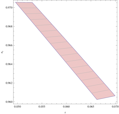
Figure 1: The parametric plot of $n_{s}$ and $r$ as functions of $\kappa^{2}h_{0}\alpha$ and $\beta/\alpha$, for $0\leq\kappa^{2}h_{0}\alpha\leq 10^{-5}$ and $0.22\leq\beta/\alpha\leq 0.26$.

This can also be seen in Fig. 2 where we present the three dimensional plot of the spectral index $n_{s}$ as a function of $\kappa^{2}h_{0}\alpha$ and $\beta/\alpha$, for $0\leq\kappa^{2}h_{0}\alpha\leq 10^{-5}$ and $0.22\leq\beta/\alpha\leq 0.26$.

In order to better understand the effect of logarithmic correction over $R^{2}$ Starobinsky inflation model, and the actual impact of the KR field on the inflationary phenomenology, let us here discuss the observational predictions of the logarithmic $R^{2}$ model in the presence or not of the KR field, and directly compare the results to the standard $R^{2}$ models for the same values of the relevant free parameters.

Let us start with the standard $R^{2}$ Starobinsky inflation model in the absence of the KR field, with the functional form of the $F(R)$ gravity being in this case $R+R^{2}/m^{2}$. The constraints for the free parameters are $0.02\lesssim m^{2}/R_{0}\lesssim 0.07$, where $R_{0}$ is the value of the the Ricci scalar at the time of horizon crossing. For these values we obtain $0.960\leq n_{s}\leq 0.970$ and $r<0.007$. With regard to the $R^{2}$ model in the presence of a Kalb-Ramond field, the constraints are $0.02\lesssim m^{2}/R_{0}\lesssim 0.07$ and $\frac{\kappa^{2}h_{0}}{m^{2}}\lesssim 3\times 10^{-3}$, and it can be shown that $n_{s}$ takes values in the range $0.95\leq n_{s}\leq 1$, while $r<0.060$. As for the logarithmic corrected $F(R)=R+R^{2}/m^{2}+\beta R^{2}\ln{(\beta R)}$ gravity without KR field, for $0.40\lesssim m^{2}/R_{0}\lesssim 0.50$ for $\beta=\frac{1}{2R_{0}}$, it can be shown that $n_{s}$ takes values in the range $0.96\leq n_{s}\leq 0.97$, while $r<0.060$. Finally, for the logarithmic corrected $R^{2}$ model with KR field, for $0.40\lesssim m^{2}/R_{0}\lesssim 0.50$, $\frac{\kappa^{2}h_{0}}{m^{2}}\lesssim 10^{-5}$ and $\beta=\frac{1}{2R_{0}}$, it can be shown that $n_{s}$ takes values in the range $0.96\leq n_{s}\leq 0.97$, while $r<0.065$. Thus the effect of the KR field is to increase the amount of gravitational radiation predicted from the standard $R^{2}$ Starobinsky inflation model.

4.2 The Constant-roll Case

In the case that the constant-roll approximation is considered, slow-roll indices are given by the following expressions, [62, 63, 64, 65],

$$\epsilon_{F} = -\frac{1}{H_{F}^{2}}\frac{dH_{F}}{d\tau},\,\,\,\,\,\epsilon_{2}=\frac{1}{2\rho_{KR}H_{F}}\frac{d\rho_{KR}}{d\tau}$$

$$\epsilon_{3} = \frac{1}{2F^{\prime}(R)H_{F}}\frac{dF^{\prime}(R)}{d\tau},\,\,\,\,\,\epsilon_{4}=\frac{1}{2EH_{F}}\frac{dE}{d\tau}\,,$$ (4.31)

and in this case, the function $E$ is equal to,

$$E=\frac{\varTheta F^{\prime}(R)H_{F}^{2}}{\rho_{KR}}\,,$$ (4.32)

where $\varTheta$ in this case, is equal to,

$$\varTheta=\frac{\rho_{KR}}{(1+\epsilon_{3})^{2}F^{\prime}(R)H_{F}^{2}}\bigg{[}F^{\prime}(R)+\frac{3}{2\kappa^{2}\rho_{KR}}\bigg{(}\frac{d}{d\tau}F^{\prime}(R)\bigg{)}^{2}\bigg{]}\,.$$ (4.33)

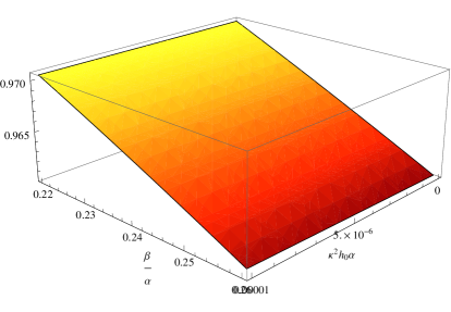
Figure 2: The three dimensional plot of the spectral index $n_{s}$ as a function of $\kappa^{2}h_{0}\alpha$ and $\beta/\alpha$, for $0\leq\kappa^{2}h_{0}\alpha\leq 10^{-5}$ and $0.22\leq\beta/\alpha\leq 0.26$.

Recall that $\rho_{KR}$ ($=H_{123}H^{123}$) denotes the energy density of the KR field in the $F(R)$ gravity model. It can easily be seen that the definitions of the slow-roll indices $\epsilon_{i}$ are the same in comparison to those corresponding to the slow-roll condition, except for the factor $(1+\epsilon_{3})^{2}$ in the denominator of $\varTheta$, however, as we will see, the resulting functional forms in terms of the model parameters $h_{0}$, $\alpha$, $\beta$, will actually change due to the constant-roll condition. The observational indices in terms of the slow-roll indices are equal to [62, 63, 64, 65],

$$n_{s}=4-2\sqrt{\bigg{[}\frac{1}{4}+\frac{\big{(}1+\epsilon_{F}+\epsilon_{2}-\epsilon_{3}+\epsilon_{4}\big{)}\big{(}2+\epsilon_{2}-\epsilon_{3}+\epsilon_{4}\big{)}}{(1-\epsilon_{F})^{2}}\bigg{]}}$$ (4.34)

and

$$r = 8\kappa^{2}\frac{\varTheta}{F^{\prime}(R)}$$ (4.35)

$$= \frac{1}{(1+\epsilon_{3})^{2}}\bigg{[}8\kappa^{2}\frac{\rho_{KR}}{F^{\prime}(R)H_{F}^{2}}+\frac{12}{F^{\prime}(R)^{2}H_{F}^{2}}\big{(}\frac{dF^{\prime}(R)}{d\tau}\big{)}^{2}\bigg{]}$$

Let us find the explicit form of each slow-roll index, so we start off with the calculation of $\epsilon_{F}$, and by using the Hubble rate of Eq. (4.4), the Hubble parameter in the $F(R)$ frame ($H_{F}$) and in the scalar-tensor frame ($H$) are related by $H_{F}=e^{-\frac{\sqrt{2}\kappa}{2\sqrt{3}}\xi(t)}\bigg{[}H+\frac{\sqrt{2}\kappa}{2\sqrt{3}}\dot{\xi}\bigg{]}$. Differentiating with respect to $\tau$ leads to the following expression,

$$\frac{dH_{F}}{d\tau} = e^{-\sqrt{\frac{2}{3}}\kappa\xi(t)}\bigg{[}\dot{H}+\frac{1}{2}\sqrt{\frac{2}{3}}\kappa\ddot{\xi}-\frac{1}{2}\sqrt{\frac{2}{3}}\kappa H\dot{\xi}-\frac{1}{6}\kappa^{2}\dot{\xi}^{2}\bigg{]}$$ (4.36)

$$= e^{-\sqrt{\frac{2}{3}}\kappa\xi(t)}\bigg{[}\dot{H}-\frac{1}{2}\sqrt{\frac{2}{3}}\kappa H\dot{\xi}(1-\gamma)-\frac{\kappa^{2}}{6}A^{2}a^{2\gamma}\bigg{]}\,,$$

where the “dot” denotes differentiation with respect to $t$, and in the second line we used the constant-roll condition. Using these expressions for $H_{F}$ and $H_{F}^{\prime}(\tau)$, we obtain the explicit form of $\epsilon_{F}$ in terms of the model parameters as follows,

$$\epsilon_{F}\bigg{|}_{\tau_{0}}=\bigg{[}\frac{\frac{3\kappa^{2}h_{0}}{2}-\frac{\kappa(1-\gamma)}{2(1+\gamma/3)}\sqrt{\frac{2}{3}}V^{\prime}(\xi)+2\kappa^{2}A^{2}a_{0}^{2\gamma}}{\kappa^{2}A^{2}a_{0}^{2\gamma}+\kappa^{2}V(\xi)+\frac{\kappa^{2}h_{0}}{2}-\frac{\kappa}{(1+\gamma/3)}\sqrt{\frac{2}{3}}V^{\prime}(\xi)}\bigg{]}$$ (4.37)

where $a_{0}=a(\tau_{0})$ and $V(\xi)$ and its derivative are given in Eqs. (3.4) and (3.7) respectively. By comparing Eqs. (4.13) and (4.37) we may conclude that $\epsilon_{F}=-H_{F}^{\prime}(\tau)/H_{F}^{2}$ differs in the slow-roll and constant-roll cases, because of the presence of $\gamma$ and $A$, as expected. Let us now turn our focus on the slow-roll parameters $\epsilon_{2}$ and $\epsilon_{3}$, and by using similar considerations, we obtain the following expressions, namely,

$$\epsilon_{2}=-3+e^{-[\frac{1}{2}\sqrt{\frac{2}{3}}\kappa\xi]}\frac{1}{2H_{F}}\sqrt{\frac{2}{3}}\kappa\dot{\xi}$$ (4.38)

and

$$\epsilon_{3} = -\epsilon_{F}$$ (4.39)

$$= -\bigg{[}\frac{\frac{3\kappa^{2}h_{0}}{2}-\frac{\kappa(1-\gamma)}{2(1+\gamma/3)}\sqrt{\frac{2}{3}}V^{\prime}(\xi)+2\kappa^{2}A^{2}a_{0}^{2\gamma}}{\kappa^{2}A^{2}a_{0}^{2\gamma}+\kappa^{2}V(\xi)+\frac{\kappa^{2}h_{0}}{2}-\frac{\kappa}{(1+\gamma/3)}\sqrt{\frac{2}{3}}V^{\prime}(\xi)}\bigg{]}\,.$$

Finally, in order to obtain $\epsilon_{4}$, recall that $E$ is defined as $E=\frac{\varTheta F^{\prime}(R)H_{F}^{2}}{\rho_{KR}}(1+\epsilon_{3})^{2}$. Differentiating with respect to $\tau$, we get,

$$\epsilon_{4} = \frac{E^{\prime}}{2EH_{F}}$$ (4.40)

$$= \frac{\varTheta^{\prime}}{2\varTheta H_{F}}+\frac{1}{2H_{F}F^{\prime}(R)}\frac{dF^{\prime}(R)}{d\tau}+\frac{H_{F}^{\prime}}{H_{F}^{2}}-\frac{\rho_{KR}^{\prime}}{2H_{F}\rho_{KR}}+\frac{\epsilon_{3}^{\prime}}{H_{F}(1+\epsilon_{3})}$$

Using Eqs. (4.38)and (4.39), the above expression can be simplified $\epsilon_{4}$ takes the following form,

$$\epsilon_{4}=\frac{\varTheta^{\prime}}{2\varTheta H_{F}}-2\epsilon_{F}-\epsilon_{2}+\frac{\epsilon_{3}^{\prime}}{H_{F}(1+\epsilon_{3})}\,.$$ (4.41)

The remaining part is to determine $\varTheta$ which is defined as,

$$\varTheta = \frac{1}{(1+\epsilon_{3})^{2}}\bigg{[}\frac{\rho_{KR}}{H_{F}^{2}}+\frac{3}{2\kappa^{2}F^{\prime}(R)H_{F}^{2}}\bigg{(}\frac{dF^{\prime}(R)}{d\tau}\bigg{)}^{2}\bigg{]}$$ (4.42)

$$= \frac{1}{(1+\epsilon_{3})^{2}}\bigg{[}\frac{\rho_{KR}}{H_{F}^{2}}+\frac{6F^{\prime}(R)\epsilon_{F}^{2}}{\kappa^{2}}\bigg{]}$$

By differentiating Eq. (4.42) and after some algebra, we obtain,

$$\frac{\varTheta^{\prime}}{2\varTheta H_{F}}+\frac{\epsilon_{3}^{\prime}}{H_{F}(1+\epsilon_{3})}=-\epsilon_{F}+\frac{\epsilon_{F}^{\prime}}{\epsilon_{F}H_{F}}+\frac{\kappa^{2}}{12\epsilon_{F}^{2}H_{F}F^{\prime}(R)}\frac{d}{d\tau}\big{[}\frac{\rho_{KR}}{H_{F}^{2}}\big{]}\,.$$ (4.43)

The evolution of $\tilde{\rho}_{KR}$ (see Eq. (3.28)) along with the conformal transformation give the variation of KR field energy density in the $F(R)$ frame, which is, $\rho_{KR}=e^{-2\sqrt{\frac{2}{3}}\kappa\xi}\frac{h_{0}}{a^{6}}$. Using this expression, Eq. (4.43) can be rewritten as follows,

$$\frac{\varTheta^{\prime}}{2\varTheta H_{F}}+\frac{\epsilon_{3}^{\prime}}{H_{F}(1+\epsilon_{3})} = -\epsilon_{F}+\frac{\epsilon_{F}^{\prime}}{\epsilon_{F}H_{F}}$$ (4.44)

$$+ \frac{\kappa^{2}\rho_{KR}}{12\epsilon_{F}^{2}H_{F}^{3}F^{\prime}(R)}\bigg{[}-6H_{F}+e^{-[\frac{1}{2}\sqrt{\frac{2}{3}}\kappa\xi]}\sqrt{\frac{2}{3}}\kappa\dot{\xi}-\frac{2H_{F}^{\prime}}{H_{F}}\bigg{]}\,.$$

Plugging back the above expression into Eq. (4.41), we obtain the final form of $\epsilon_{4}$, which is,

$$\epsilon_{4} = -\epsilon_{2}-3\epsilon_{F}+\frac{\epsilon_{F}^{\prime}}{\epsilon_{F}H_{F}}$$ (4.45)

$$+ \frac{\kappa^{2}\rho_{KR}}{12\epsilon_{F}^{2}H_{F}^{3}F^{\prime}(R)}\bigg{[}-6H_{F}+e^{-[\frac{1}{2}\sqrt{\frac{2}{3}}\kappa\xi]}\sqrt{\frac{2}{3}}\kappa\dot{\xi}-\frac{2H_{F}^{\prime}}{H_{F}}\bigg{]}\,.$$

In view of the above resulting expressions, the spectral index and the tensor-to-scalar ratio in the constant-roll approximation read,

$$n_{s}=4-2\sqrt{\frac{1}{4}+\frac{D_{1}D_{2}}{D_{3}}}\,,$$ (4.46)

and

$$r=\frac{D_{4}}{(1+\epsilon_{3})^{2}}\,,$$ (4.47)

where the functions $D_{i}$ are defined as follows,

$$D_{1} =1+\epsilon_{F}+\epsilon_{2}-\epsilon_{3}+\epsilon_{4}$$ (4.48)

$$= 1-\bigg{[}\frac{\frac{3\kappa^{2}h_{0}}{2}-\frac{\kappa(1-\gamma)}{2(1+\gamma/3)}\sqrt{\frac{2}{3}}V^{\prime}(\xi)+2\kappa^{2}A^{2}a_{0}^{2\gamma}}{\kappa^{2}A^{2}a_{0}^{2\gamma}+\kappa^{2}V(\xi)+\frac{\kappa^{2}h_{0}}{2}-\frac{\kappa}{(1+\gamma/3)}\sqrt{\frac{2}{3}}V^{\prime}(\xi)}\bigg{]}+\bigg{[}\frac{-\frac{\kappa^{2}h_{0}}{2}+\frac{1}{72}\bigg{(}\frac{\sqrt{2/3}\frac{\kappa}{(1+\gamma/3)^{2}}V^{\prime}(\xi)V^{\prime\prime}(\xi)}{\kappa^{2}V(\xi)+\kappa^{2}h_{0}/2}\bigg{)}}{\frac{3\kappa^{2}h_{0}}{2}-\frac{\kappa(1-\gamma)}{2(1+\gamma/3)}\sqrt{2/3}V^{\prime}(\xi)+2\kappa^{2}A^{2}}\bigg{]}$$

$$+ \bigg{[}\frac{\frac{3\kappa^{2}h_{0}}{2}+\frac{1}{72}\bigg{(}\frac{\big{(}\sqrt{2/3}\frac{\kappa}{(1+\gamma/3)}V^{\prime}(\xi)\big{)}^{2}}{\kappa^{2}V(\xi)+\kappa^{2}h_{0}/2}\bigg{)}}{\frac{\kappa^{2}h_{0}}{2}-\frac{\kappa}{(1+\gamma/3)}\sqrt{2/3}V^{\prime}(\xi)+\kappa^{2}V(\xi)+\kappa^{2}A^{2}}\bigg{]}$$

$$- \bigg{[}\frac{3\kappa^{2}h_{0}}{8\big{[}2\alpha+\beta+2\beta\ln{(\beta R_{0})}\big{]}\big{[}\frac{3\kappa^{2}h_{0}}{2}-\frac{\kappa(1-\gamma)}{2(1+\gamma/3)}\sqrt{2/3}V^{\prime}(\xi)+2\kappa^{2}A^{2}\big{]}^{2}}\bigg{]}$$

$$+ \bigg{[}\frac{\kappa^{2}h_{0}/\big{[}2\alpha+\beta+2\beta\ln{(\beta R_{0})}\big{]}}{8\big{[}\frac{3\kappa^{2}h_{0}}{2}-\frac{\kappa(1-\gamma)}{2(1+\gamma/3)}\sqrt{2/3}V^{\prime}(\xi)+2\kappa^{2}A^{2}\big{]}\big{[}\kappa^{2}V(\xi)+\frac{\kappa^{2}h_{0}}{2}-\frac{\kappa}{(1+\gamma/3)}\sqrt{2/3}V^{\prime}(\xi)+\kappa^{2}A^{2}}\bigg{]}\,,$$

$$D_{2} = 2+\epsilon_{F}+\epsilon_{2}+\epsilon_{4}$$ (4.49)

$$= 1+D_{1}-\epsilon_{F}$$

$$= 1+D_{1}-\bigg{[}\frac{\frac{3\kappa^{2}h_{0}}{2}-\frac{\kappa(1-\gamma)}{2(1+\gamma/3)}\sqrt{\frac{2}{3}}V^{\prime}(\xi)+2\kappa^{2}A^{2}a_{0}^{2\gamma}}{\kappa^{2}A^{2}a_{0}^{2\gamma}+\kappa^{2}V(\xi)+\frac{\kappa^{2}h_{0}}{2}-\frac{\kappa}{(1+\gamma/3)}\sqrt{\frac{2}{3}}V^{\prime}(\xi)}\bigg{]}\,,$$

$$D_{3} = (1-\epsilon_{F})^{2}$$ (4.50)

$$= \bigg{[}1-\bigg{(}\frac{\frac{3\kappa^{2}h_{0}}{2}-\frac{\kappa(1-\gamma)}{2(1+\gamma/3)}\sqrt{\frac{2}{3}}V^{\prime}(\xi)+2\kappa^{2}A^{2}a_{0}^{2\gamma}}{\kappa^{2}A^{2}a_{0}^{2\gamma}+\kappa^{2}V(\xi)+\frac{\kappa^{2}h_{0}}{2}-\frac{\kappa}{(1+\gamma/3)}\sqrt{\frac{2}{3}}V^{\prime}(\xi)}\bigg{)}\bigg{]}^{2}\,,$$

$$D_{4} = 8\kappa^{2}\frac{\rho_{KR}}{F^{\prime}(R)H_{F}^{2}}+\frac{12}{F^{\prime}(R)^{2}H_{F}^{2}}\bigg{(}\frac{dF^{\prime}(R)}{d\tau}\bigg{)}^{2}$$ (4.51)

$$= \frac{\frac{6\kappa^{2}h_{0}\alpha}{(2+\beta/\alpha)}+48\bigg{(}\frac{3\kappa^{2}h_{0}\alpha}{2}+\frac{\kappa^{2}A^{2}\alpha}{2}\bigg{)}^{2}}{\bigg{(}\frac{1}{8(1+\beta/\alpha)}+\frac{\kappa^{2}h_{0}\alpha}{2}+\kappa^{2}A^{2}\alpha\bigg{)}^{2}}\,.$$

From the above expressions, it is clear that the observational indices depend on the free parameters $\alpha$, $\beta$, $h_{0}$, $R_{0}$, $\gamma$ and $A$ where the last two arise due to the constant-roll condition. As in the slow-roll case, we shall assume that $\alpha\neq\beta\sim 1/R_{0}$, and also the parameter $A$ is fixed in order for the expression $\kappa A\sqrt{\alpha}$ to be equal to one, that is $\kappa A\sqrt{\alpha}=1$. In effect, the spectral index $n_{s}$ and the tensor-to-scalar ratio $r$ depend solely on the two dimensionless parameters $\kappa^{h}_{0}\alpha$, $\beta/\alpha$, $\gamma$ and $\kappa^{2}A^{2}\alpha$. By exploring the parameter space, we found that the observational indices are compatible with the Planck 2018 and the BICEP2/Keck-Array data when the values of the parameters are constrained by the bound $\kappa^{2}h_{0}\alpha\bigg{|}_{max}=5\times 10^{-5}$, which is in agreement to the one obtained by the slow-roll approximation, and also for $\frac{\beta}{\alpha}\simeq[0.25,0.30]$. The latter constraint, clearly demonstrates that the ratio $\beta/\alpha$ takes more restricted values in the constant-roll case. We summarize the results in Table[2].

Constraints in slow-roll condition	Constraints in constant-roll condition
$\big{(}\frac{\kappa^{2}h_{0}}{\alpha}\big{)}_{max}\simeq 10^{-5}$	$\big{(}\frac{\kappa^{2}h_{0}}{\alpha}\big{)}_{max}\simeq 5\times 10^{-5}$ (for $\gamma=0.01$)
$\frac{\beta}{\alpha}\simeq[0.20,0.25]$	$\frac{\beta}{\alpha}\simeq[0.25,0.30]$ (for $\gamma=0.01$)

Table 2: Constraints on various parameters in slow-roll as well as in constant-roll condition

Therefore the present scenario successfully provides a viable inflationary phenomenology, which is compatible with the $Planck$ 2018 and BICEP2/Keck-Array data, with the difference from the constant-roll case being that the ratio $\beta/\alpha$ is more constrained in the constant-roll case. We can also see the simultaneous compatibility of the spectral index and of the tensor-to-scalar ratio in Fig. 3 where we present the parametric plot of $n_{s}$ and $r$ as functions of $\kappa^{2}h_{0}\alpha$ and $\beta/\alpha$, for $0\leq\kappa^{2}h_{0}\leq\alpha 10^{-5}$ and $0.25\leq\beta/\alpha\leq 0.30$. As it can be seen from Fig. 3, there exist a wide range of the free parameters for which the simultaneous compatibility of the spectral index and of the tensor-to-scalar ratio can be achieved.

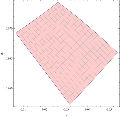
Figure 3: The parametric plot of $n_{s}$ and $r$ as functions of $\kappa^{2}h_{0}\alpha$ and $\beta/\alpha$, for $0\leq\kappa^{2}h_{0}\alpha\leq 5\times 10^{-5}$ and $0.25\leq\beta/\alpha\leq 0.30$.

As in the slow-roll case, it is worth comparing the standard $R^{2}$ Starobinsky inflation phenomenology with the logarithmic $R^{2}$ model in the presence or not of a KR field. Recall that the standard $R^{2}$ model $F(R)=R+R^{2}/m^{2}$ is viable for $0.07\lesssim m^{2}/R_{0}\lesssim 0.13$, with $R_{0}$, and it yields $0.960\leq n_{s}\leq 0.970$ and $r<0.02$. For the constant-roll case of the $R^{2}$ model in the presence of a KR field, viable results are obtained for $0.07\lesssim m^{2}/R_{0}\lesssim 0.13$ and $\frac{\kappa^{2}h_{0}}{m^{2}}\lesssim 10^{-4}$, and particularly $n_{s}$ takes values in the range $0.959\leq n_{s}\leq 0.972$, and $r<0.04$. For the logarithmic corrected $R^{2}$ model, in the absence of the KR field, for $0.50\lesssim m^{2}/R_{0}\lesssim 0.60$ and $\beta=\frac{1}{2R_{0}}$, the spectral index $n_{s}$ takes values in the range $0.958\leq n_{s}\leq 0.969$, and $r<0.03$. Finally for the logarithmic corrected model in the presence of a KR field, for $0.50\lesssim m^{2}/R_{0}\lesssim 0.60$, $\frac{\kappa^{2}h_{0}}{m^{2}}\lesssim 5\times 10^{-5}$ and $\beta=\frac{1}{2R_{0}}$, $n_{s}$ takes values in the range $0.959\leq n_{s}\leq 0.974$, and $r<0.05$. Thus the KR field effect is to induce a larger amount of gravitational radiation in comparison to the standard $R^{2}$ model.

5 Conclusions

In this paper we considered a logarithmic modification of the standard $R^{2}$ Starobinsky inflation, of the form, $F(R)=R+\alpha R^{2}+\beta R^{2}\ln{(\beta R)}$ which is motivated by one-loop corrected higher derivative gravity, in the presence of a rank two antisymmetric tensor field, popularly known as Kalb-Ramond field. The model is free from ghost fields if $\alpha$, $\beta$ $>0$. Also the Kalb-Ramond effects are strong during the large curvature regime, but these reduce as the Universe expands, at a rate $\sim a^{-6}$, and in effect, radiation and matter dominate the post-inflationary phase of our Universe. We focused on the inflationary aspects of the model, and we calculated in detail the observational indices of the model, in two approximating cases, namely under the slow-roll condition and under the constant-roll condition. It turns out that for both the slow-roll and constant-roll cases, the theoretical values of $n_{s}$, $r$ match the observational constraints if the values of $h_{0}$ and $\alpha$ take values that are bounded from above by the constraint $\kappa^{2}h_{0}\alpha\bigg{|}_{max}=5\times 10^{-5}$, where $h_{0}$ denotes the energy density of the Kalb-Ramond field. However the ratio $\beta/\alpha$ is constrained in different ways, in the slow-roll and constant-roll cases, with the constant-roll constraint being $0.25<\frac{\beta}{\alpha}\lesssim 0.30$ and the slow-roll one being $0.20<\frac{\beta}{\alpha}\lesssim 0.25$. In addition, our theoretical framework puts an upper bound in the value of $h_{0}$, which can be obtained by fixing $\alpha=1$ in Planck units, and this leads to $h_{0}^{max}\sim 10^{71}$ (GeV)⁴, so in effect, the Kalb-Ramond field energy density is constrained as follows $\big{(}\rho_{KR}\big{)}^{max}\sim 10^{71}$ (GeV)⁴. Moreover, let us note that the effect of the KR field on the inflationary phenomenology of $R^{2}$ Starobinsky inflation and logarithmic $R^{2}$ gravity is that it increases the amount of the primordial gravitational radiation. As a generalization of this work, one should consider the effects of a massive antisymmetric field [26] on $F(R)$ gravity inflation, and we hope to address this issue in a future work.

Finally we need to stress an important issue, the fact that in the context of our work, there is a direct correspondence between the massless KR field and the massless scalar field at the level of cosmological background and linear cosmological perturbations (with the latter perturbations equivalence being considered with caution and only at linear order). Particularly, the correspondence is materialized by the equivalence of the Eqs. (3.45 - 3.51) and Eqs. (3.53 - 3.59), which can be used as a recipe to go between the two pictures. This correspondence recipe, at this level of the analysis, allows to obtain all the results for KR fields in inflation directly from the massless scalar results which are considerably simpler to calculate. Indeed the equivalence is justified due to the fact that, $H_{\mu\nu\alpha}=\epsilon_{\mu\nu\rho\sigma}\partial^{\sigma}Z$ (with $H_{\mu\nu\alpha}$ and $Z$ being the KR tensor and the scalar field respectively) which can be indeed used as a recipe to go between the two pictures. Thereby this correspondence relation allows one to obtain the expression of inflationary parameters with KR field directly from massless scalar case, which are relatively simpler to compute, as we already mentioned. Furthermore, in the present context as we are interested on inflationary parameters like spectral index and tensor to scalar ratio, so we demonstrated the equivalence only up to first order perturbation equations and we did not consider the higher order perturbations. However the investigation of such equivalence for second (or higher) order perturbations is important from its own right, and non-trivial, so we hope to address in a future work. Also, we should note that we studied free KB tensors, but in principle we can also take into account potential terms for them, and /or we can consider a direct non-minimal coupling of such fields with curvature for example of the form $G(F^{2})f(R)$, where $F^{2}$ is the square of such tensors. In this case, the background equivalence is in general lost and the results would completely different from the case we studied in this paper, in which only non-minimal couplings were considered. This extension will be considered elsewhere.

Appendix: The Time Dependence of the Kalb-Ramond Field and Equivalence of Field Equations

Due to antisymmetric nature, $\tilde{H}_{\mu\nu\alpha}$ has four independent components in four dimensions and thus it can be equivalently expressed as a vector field as follows,

$$\tilde{H}_{\mu\nu\alpha}=\varepsilon_{\mu\nu\alpha\beta}\Upsilon^{\beta}\,,$$ (5.1)

where $\varepsilon_{\mu\nu\alpha\beta}$ is the Levi-Civita symbol and $\Upsilon^{\beta}$ is a vector field propagating in four dimensional spacetime. The four components of $\Upsilon^{\beta}$ are connected with the independent components of $\tilde{H}_{\mu\nu\alpha}$ as follows,

$$\tilde{H}_{012}=h_{1}=\Upsilon^{3},\,\,\,\,\,\,\tilde{H}_{013}=h_{2}=-\Upsilon^{2}$$

$$\tilde{H}_{023}=h_{3}=\Upsilon^{1},\,\,\,\,\,\,\tilde{H}_{123}=h_{4}=-\Upsilon^{0}\,.$$ (5.2)

By using a FRW background, the off-diagonal Friedmann equations become,

$$\Upsilon_{3}\Upsilon^{2}=\Upsilon_{3}\Upsilon^{1}=\Upsilon_{2}\Upsilon^{1}=\Upsilon_{0}\Upsilon^{3}=\Upsilon_{0}\Upsilon^{2}=\Upsilon_{0}\Upsilon^{1}=0\,.$$ (5.3)

The above set of equations clearly indicate that only one component of $\Upsilon^{\beta}$ is non-zero, which in turn reduces the independent components of $\tilde{H}_{\mu\nu\alpha}$ to one. Therefore, in the present context (i.e. for spatially flat FRW metric in four dimensions), $\Upsilon^{\beta}$ can be expressed as a derivative of a massless scalar field $Z(x^{\mu})$ (i.e $\Upsilon^{\beta}=\partial^{\beta}Z$), which further relates the KR field tensor with the scalar field in the following way,

$$\tilde{H}_{\mu\nu\alpha} = \varepsilon_{\mu\nu\alpha\beta}\Upsilon^{\beta}$$ (5.4)

$$= \varepsilon_{\mu\nu\alpha\beta}\partial^{\beta}Z$$

For the FRW metric, the scalar field ($Z$) is spatially homogeneous and in effect, its equation of motion turns out to be,

$$\ddot{Z}+3H\dot{Z}=0\,.$$ (5.5)

where $H$ is the Hubble parameter. Solving the above equation, one obtains,

$$\frac{\partial Z}{\partial t}\propto\frac{1}{a^{3}}=\frac{d}{a^{3}}$$ (5.6)

where $d$ is an integration constant. With this solution of $\frac{\partial Z}{\partial t}$, the diagonal Friedmann equations take the following form,

$$H^{2} = \frac{\kappa^{2}}{3}\bigg{[}\frac{1}{2}\dot{\xi}^{2}+\frac{m^{2}}{8\kappa^{2}}\big{(}1-e^{\sqrt{\frac{2}{3}}\kappa\xi}\big{)}^{2}+\frac{1}{2}\dot{Z}^{2}\bigg{]}$$ (5.7)

$$= \frac{\kappa^{2}}{3}\bigg{[}\frac{1}{2}\dot{\xi}^{2}+\frac{m^{2}}{8\kappa^{2}}\big{(}1-e^{\sqrt{\frac{2}{3}}\kappa\xi}\big{)}^{2}+\frac{d}{2a^{6}}\bigg{]}\,,$$

and

$$2\dot{H}+3H^{2}=-\kappa^{2}\bigg{[}\frac{1}{2}\dot{\xi}^{2}-\frac{m^{2}}{8\kappa^{2}}\bigg{(}1-e^{\sqrt{\frac{2}{3}}\kappa\xi}\bigg{)}^{2}+\frac{1}{2}\dot{Z}^{2}\bigg{]}$$

$$=-\kappa^{2}\bigg{[}\frac{1}{2}\dot{\xi}^{2}-\frac{m^{2}}{8\kappa^{2}}\bigg{(}1-e^{\sqrt{\frac{2}{3}}\kappa\xi}\bigg{)}^{2}+\frac{d}{2a^{6}}\bigg{]}\,,$$ (5.8)

and recall, $\xi(t)$ is the scalar field arises from the higher curvature degree of freedom. Furthermore, the field equation for $\xi(t)$ is given by,

$$\ddot{\xi}+3H\dot{\xi}-\sqrt{\frac{2}{3}}\frac{m^{2}}{4\kappa}e^{\sqrt{\frac{2}{3}}\kappa\xi}\big{(}1-e^{\sqrt{\frac{2}{3}}\kappa\xi}\big{)}=0\,.$$ (5.9)

As it can be seen the above equations match the field equations appearing in Eqs. (3.29), (3.30), by identifying the constant $d$ with $h_{0}$. This leads to the argument that the field equations of the KR field obtained with and without expressing the KR as a vector field, are equivalent.

References

- [1] A. H. Guth, Phys. Rev. D 23 (1981) 347. doi:10.1103/PhysRevD.23.347
- [2] A. A. Starobinsky, Phys. Lett. B 91 (1980) 99 [Phys. Lett. 91B (1980) 99] [Adv. Ser. Astrophys. Cosmol. 3 (1987) 130]. doi:10.1016/0370-2693(80)90670-X
- [3] A. R. R. Castellanos, F. Sobreira, I. L. Shapiro and A. A. Starobinsky, arXiv:1810.07787 [gr-qc].
- [4] S. J. Wang, arXiv:1810.06445 [hep-th].
- [5] A. D. Linde, Phys. Lett. 129B (1983) 177. doi:10.1016/0370-2693(83)90837-7
- [6] A. D. Linde, Lect. Notes Phys. 738 (2008) 1 [arXiv:0705.0164 [hep-th]].
- [7] D. S. Gorbunov and V. A. Rubakov, “Introduction to the theory of the early universe: Cosmological perturbations and inflationary theory,” Hackensack, USA: World Scientific (2011) 489 p;
- [8] D. H. Lyth and A. Riotto, Phys. Rept. 314 (1999) 1 [hep-ph/9807278].
-
[9]
R. Brandenberger and P. Peter,
Found. Phys. 47 (2017) no.6, 797
doi:10.1007/s10701-016-0057-0
[arXiv:1603.05834 [hep-th]].;
J. de Haro and Y. F. Cai, Gen. Rel. Grav. 47 (2015) no.8, 95 doi:10.1007/s10714-015-1936-y [arXiv:1502.03230 [gr-qc]].;
Y. F. Cai, Sci. China Phys. Mech. Astron. 57 (2014) 1414 doi:10.1007/s11433-014-5512-3 [arXiv:1405.1369 [hep-th]]. - [10] Y. Akrami et al. [Planck Collaboration], arXiv:1807.06211 [astro-ph.CO].
- [11] P. A. R. Ade et al. [BICEP2 and Keck Array Collaborations], Phys. Rev. Lett. 116 (2016) 031302 doi:10.1103/PhysRevLett.116.031302 [arXiv:1510.09217 [astro-ph.CO]].
- [12] S. Nojiri, S. D. Odintsov and V. K. Oikonomou, Phys. Rept. 692 (2017) 1 doi:10.1016/j.physrep.2017.06.001 [arXiv:1705.11098 [gr-qc]].
- [13] S. Nojiri, S.D. Odintsov, Phys. Rept. 505, 59 (2011);
- [14] S. Nojiri, S.D. Odintsov, eConf C0602061, 06 (2006) [Int. J. Geom. Meth. Mod. Phys. 4, 115 (2007)].
-
[15]
S. Capozziello, M. De Laurentis,
Phys. Rept. 509, 167 (2011);
V. Faraoni and S. Capozziello, Fundam. Theor. Phys. 170 (2010). doi:10.1007/978-94-007-0165-6 - [16] A. de la Cruz-Dombriz and D. Saez-Gomez, Entropy 14 (2012) 1717 doi:10.3390/e14091717 [arXiv:1207.2663 [gr-qc]].
- [17] G. J. Olmo, Int. J. Mod. Phys. D 20 (2011) 413 doi:10.1142/S0218271811018925 [arXiv:1101.3864 [gr-qc]].
- [18] S. Nojiri and S. D. Odintsov, Phys. Rev. D 68 (2003) 123512 doi:10.1103/PhysRevD.68.123512 [hep-th/0307288].
- [19] S. D. Odintsov, V. K. Oikonomou and L. Sebastiani, Nucl. Phys. B 923 (2017) 608 doi:10.1016/j.nuclphysb.2017.08.018 [arXiv:1708.08346 [gr-qc]].
- [20] S. D. Odintsov, D. Saez-Chillon Gomez and G. S. Sharov, arXiv:1807.02163 [gr-qc].
- [21] S. Nojiri and S. D. Odintsov, Gen. Rel. Grav. 36 (2004) 1765 doi:10.1023/B:GERG.0000035950.40718.48 [hep-th/0308176].
- [22] G. Cognola, E. Elizalde, S. Nojiri, S. D. Odintsov and S. Zerbini, JCAP 0502 (2005) 010 doi:10.1088/1475-7516/2005/02/010 [hep-th/0501096].
- [23] E. Elizalde, S. D. Odintsov, L. Sebastiani and R. Myrzakulov, Nucl. Phys. B 921 (2017) 411 doi:10.1016/j.nuclphysb.2017.06.003 [arXiv:1706.01879 [gr-qc]].
- [24] R. Myrzakulov, S. Odintsov and L. Sebastiani, Phys. Rev. D 91 (2015) no.8, 083529 doi:10.1103/PhysRevD.91.083529 [arXiv:1412.1073 [gr-qc]].
- [25] L. H. Liu, T. Prokopec and A. A. Starobinsky, Phys. Rev. D 98 (2018) no.4, 043505 doi:10.1103/PhysRevD.98.043505 [arXiv:1806.05407 [gr-qc]].
- [26] I. L. Buchbinder, E. N. Kirillova and N. G. Pletnev, Phys. Rev. D 78 (2008) 084024 doi:10.1103/PhysRevD.78.084024 [arXiv:0806.3505 [hep-th]].
- [27] A. Das, T. Paul and S. Sengupta, arXiv:1804.06602 [hep-th].
- [28] S. Inoue and J. Yokoyama, Phys. Lett. B 524 (2002) 15 doi:10.1016/S0370-2693(01)01369-7 [hep-ph/0104083].
- [29] N. C. Tsamis and R. P. Woodard, Phys. Rev. D 69 (2004) 084005 doi:10.1103/PhysRevD.69.084005 [astro-ph/0307463].
- [30] W. H. Kinney, Phys. Rev. D 72 (2005) 023515 doi:10.1103/PhysRevD.72.023515 [gr-qc/0503017].
- [31] K. Tzirakis and W. H. Kinney, Phys. Rev. D 75 (2007) 123510 doi:10.1103/PhysRevD.75.123510 [astro-ph/0701432].
- [32] M. H. Namjoo, H. Firouzjahi and M. Sasaki, Europhys. Lett. 101 (2013) 39001 doi:10.1209/0295-5075/101/39001 [arXiv:1210.3692 [astro-ph.CO]].
- [33] J. Martin, H. Motohashi and T. Suyama, Phys. Rev. D 87 (2013) no.2, 023514 doi:10.1103/PhysRevD.87.023514 [arXiv:1211.0083 [astro-ph.CO]].
- [34] H. Motohashi, A. A. Starobinsky and J. Yokoyama, JCAP 1509 (2015) no.09, 018 doi:10.1088/1475-7516/2015/09/018 [arXiv:1411.5021 [astro-ph.CO]].
- [35] Y. F. Cai, J. O. Gong, D. G. Wang and Z. Wang, JCAP 1610 (2016) no.10, 017 doi:10.1088/1475-7516/2016/10/017 [arXiv:1607.07872 [astro-ph.CO]].
- [36] H. Motohashi and A. A. Starobinsky, arXiv:1702.05847 [astro-ph.CO].
- [37] S. Hirano, T. Kobayashi and S. Yokoyama, Phys. Rev. D 94 (2016) no.10, 103515 doi:10.1103/PhysRevD.94.103515 [arXiv:1604.00141 [astro-ph.CO]].
- [38] L. Anguelova, Nucl. Phys. B 911 (2016) 480 doi:10.1016/j.nuclphysb.2016.08.020 [arXiv:1512.08556 [hep-th]].
- [39] J. L. Cook and L. M. Krauss, JCAP 1603 (2016) no.03, 028 doi:10.1088/1475-7516/2016/03/028 [arXiv:1508.03647 [astro-ph.CO]].
- [40] K. S. Kumar, J. Marto, P. Vargas Moniz and S. Das, JCAP 1604 (2016) no.04, 005 doi:10.1088/1475-7516/2016/04/005 [arXiv:1506.05366 [gr-qc]].
- [41] S. D. Odintsov and V. K. Oikonomou, arXiv:1703.02853 [gr-qc].
- [42] S. D. Odintsov and V. K. Oikonomou, arXiv:1704.02931 [gr-qc].
- [43] J. Lin, Q. Gao and Y. Gong, Mon. Not. Roy. Astron. Soc. 459 (2016) no.4, 4029 doi:10.1093/mnras/stw915 [arXiv:1508.07145 [gr-qc]].
- [44] Q. Gao and Y. Gong, arXiv:1703.02220 [gr-qc].
- [45] S. Nojiri, S. D. Odintsov and V. K. Oikonomou, Class. Quant. Grav. 34 (2017) no.24, 245012 doi:10.1088/1361-6382/aa92a4 [arXiv:1704.05945 [gr-qc]].
- [46] H. Motohashi and A. A. Starobinsky, Eur. Phys. J. C 77 (2017) no.8, 538 doi:10.1140/epjc/s10052-017-5109-x [arXiv:1704.08188 [astro-ph.CO]].
- [47] Q. Gao, Sci. China Phys. Mech. Astron. 60 (2017) no.9, 090411 doi:10.1007/s11433-017-9065-4 [arXiv:1704.08559 [astro-ph.CO]].
- [48] F. Cicciarella, J. Mabillard and M. Pieroni, JCAP 1801 (2018) no.01, 024 doi:10.1088/1475-7516/2018/01/024 [arXiv:1709.03527 [astro-ph.CO]].
- [49] A. Awad, W. El Hanafy, G. G. L. Nashed, S. D. Odintsov and V. K. Oikonomou, JCAP 1807 (2018) no.07, 026 doi:10.1088/1475-7516/2018/07/026 [arXiv:1710.00682 [gr-qc]].
- [50] L. Anguelova, P. Suranyi and L. C. R. Wijewardhana, JCAP 1802 (2018) no.02, 004 doi:10.1088/1475-7516/2018/02/004 [arXiv:1710.06989 [hep-th]].
- [51] A. Ito and J. Soda, Eur. Phys. J. C 78 (2018) no.1, 55 doi:10.1140/epjc/s10052-018-5534-5 [arXiv:1710.09701 [hep-th]].
- [52] A. Karam, L. Marzola, T. Pappas, A. Racioppi and K. Tamvakis, JCAP 1805 (2018) no.05, 011 doi:10.1088/1475-7516/2018/05/011 [arXiv:1711.09861 [astro-ph.CO]].
- [53] Z. Yi and Y. Gong, JCAP 1803 (2018) no.03, 052 doi:10.1088/1475-7516/2018/03/052 [arXiv:1712.07478 [gr-qc]].
- [54] A. Mohammadi, K. Saaidi and T. Golanbari, Phys. Rev. D 97 (2018) no.8, 083006 doi:10.1103/PhysRevD.97.083006 [arXiv:1801.03487 [hep-ph]].
- [55] Q. Gao, Y. Gong and Q. Fei, JCAP 1805 (2018) no.05, 005 doi:10.1088/1475-7516/2018/05/005 [arXiv:1801.09208 [gr-qc]].
- [56] Q. Gao, Sci. China Phys. Mech. Astron. 61 (2018) no.7, 070411 doi:10.1007/s11433-018-9197-2 [arXiv:1802.01986 [gr-qc]].
- [57] M. J. P. Morse and W. H. Kinney, Phys. Rev. D 97 (2018) no.12, 123519 doi:10.1103/PhysRevD.97.123519 [arXiv:1804.01927 [astro-ph.CO]].
- [58] A. Mohammadi, K. Saaidi and T. Golanbari, arXiv:1808.07246 [gr-qc].
- [59] B. Boisseau and H. Giacomini, arXiv:1809.09169 [gr-qc].
- [60] I. L. Buchbinder, S. D. Odintsov and I. L. Shapiro, “Effective action in quantum gravity,” Bristol, UK: IOP (1992) 413 p
- [61] S. Chakraborty and S. Sengupta, JCAP 1805 (2018) no.05, 032 doi:10.1088/1475-7516/2018/05/032 [arXiv:1708.08315 [gr-qc]].
- [62] H. Noh and J. c. Hwang, Phys. Lett. B 515 (2001) 231 doi:10.1016/S0370-2693(01)00875-9 [astro-ph/0107069].
- [63] J. c. Hwang and H. Noh, Phys. Rev. D 71 (2005) 063536 doi:10.1103/PhysRevD.71.063536 [gr-qc/0412126].
- [64] J. c. Hwang and H. Noh, Phys. Rev. D 66 (2002) 084009 doi:10.1103/PhysRevD.66.084009 [hep-th/0206100].
- [65] D. I. Kaiser and E. I. Sfakianakis, Phys. Rev. Lett. 112 (2014) no.1, 011302 doi:10.1103/PhysRevLett.112.011302 [arXiv:1304.0363 [astro-ph.CO]].