Topological Amorphous Metals

Abstract

We study amorphous systems with completely random sites and find that, through constructing and exploring a concrete model Hamiltonian, such a system can host an exotic phase of topological amorphous metal in three dimensions. In contrast to the traditional Weyl semimetals, topological amorphous metals break translational symmetry, and thus cannot be characterized by the first Chern number defined based on the momentum space band structures. Instead, their topological properties will manifest in the Bott index and the Hall conductivity as well as the surface states. By studying the energy band and quantum transport properties, we find that topological amorphous metals exhibit a diffusive metal behavior. We further introduce a practical experimental proposal with electric circuits where the predicted phenomena can be observed using state-of-the-art technologies. Our results open a door for exploring topological gapless phenomena in amorphous systems.

Weyl semimetals, three-dimensional (3D) materials with Weyl points in band structures Burkov2016 ; Jia2016 ; VishwanathRMP ; XuReview , have attracted considerable interest Wan2011prb ; Yuanming2011PRB ; Burkov2011PRL ; ZhongFang2011prl ; Bergholtz2014PRL ; Tena2015RPL ; Bergholtz2015PRL ; Weng2015PRX ; Shengyuan2015 ; Xie2015PRL ; Xu2015 ; Lv2015 ; Lu2015 ; Zhangyi2016SciRep ; Pixley2016PRX ; Ueda2016 ; Yong2016typeii ; Pixley2018PRL ; Syzranov2018 in recent years owing to their fundamental importance in mimicking Weyl fermions in particle physics and their exotic topological properties. In the context of solid-state materials, the linear energy band dispersion around a Weyl point determines the semimetal property with a zero density of states (DOS) at zero energy. In addition, the Weyl point is protected by the first Chern number defined by the integral of Berry curvatures over a closed surface in momentum space enclosing the point volovik , leading to a Fermi arc consisting of surface states. This topological feature gives rise to the topological anomalous Hall effect Yuanming2011PRB ; Burkov2011PRL . Beyond Weyl fermions that exist in particle physics, new fermions, such as type II Weyl fermions Soluyanov2015Nature ; Shuyun2016 ; Huang2016 (also called structured Weyl fermions Yong2015PRL ) and high spin fermions Bernevig2016Science ; HongDing2017Nature , can appear in topological gapless materials.

All these topological gapless materials feature the existence of gapless structures in momentum space so that the topological invariants can be further defined there. Yet, this can only be guaranteed in a crystalline material with translational symmetry. Here, we ask whether a topological semimetal or metal can exist in an amorphous system with completely random sites, such as glass materials, where the desired translational symmetry is absent. Recent development of technologies in engineering in quantum systems such as arbitrary positioning of atoms Browaeys2016Science ; Lukin2016Science and in mechanical systems such as constructing interacting gyroscopes  MitchellNat2018 have paved the way for fabricating amorphous materials. However, the study of topological phenomena in amorphous systems is still in its infancy stage and only a few works demonstrating the existence of topological insulators in amorphous systems has been reported Shenoy2017PRL ; MitchellNat2018 ; Ojanen2018NatCommun ; Chong2017PRB ; Xiao2017PRB ; Prodan2018 ; Minarelli2018 ; Chern2018 . Whether topological semimetals or metals exist in amorphous systems have not been explored hitherto.

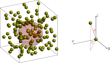
Figure 1: (Color online) Schematic of a 3D random site configuration with the allowed hopping inside the light red sphere for a typical site at the center.

In this paper, we demonstrate, by constructing and exploring a model Hamiltonian, the existence of a topological metal phase in a 3D amorphous system. The system is generated by randomly sampling sites in a box (see Fig. 1 for one sample configuration) and the results are obtained by averaging over many sample configurations. We find three distinct phases, namely, the topological amorphous metal (TAM), the amorphous Anderson insulator (AAI), and the amorphous insulator (AI) phases. In contrast to Weyl semimetals with translational symmetry where their topology can be characterized by the first Chern number, the topological feature of our amorphous system is identified using the Bott index, the Hall conductivity and the surface states. To determine whether a phase in the amorphous system is a metal, a semimetal or an insulator, we compute the band properties including the energy gap, the DOS, the level statistics and the inverse participation ratio, and the transport properties including the longitudinal conductivity and the Fano factor. We find that, in the most part of the parameter region where the Bott index and the Hall conductivity are nonzero, the system is gapless, exhibiting a diffusive metal behavior. The other regions correspond to the insulating phase where the longitudinal conductivity drops to zero and the Fano factor suddenly rises to one. The insulator can be further divided into the AAI with a nonzero DOS and the AI with a zero DOS. Finally, we introduce a practical scheme to realize such a Hamiltonian and observe its related exotic phenomena in electric circuits.

Model Hamiltonian.— We start by constructing the following model Hamiltonian

$$H=\sum_{\bf x}[\sum_{\bf R}t(R)\hat{c}_{\bf x}^{\dagger}H_{0}(\theta,\phi)\hat{c}_{{\bf x}+{\bf R}(\theta,\phi)}+m_{z}\hat{c}_{\bf x}^{\dagger}\sigma_{z}\hat{c}_{\bf x}],$$ (1)

where $\hat{c}_{\bf x}^{\dagger}=(\hat{c}_{{\bf x},\uparrow}^{\dagger},\hat{c}_{{\bf x},\downarrow}^{\dagger})$ with $\hat{c}_{{\bf x},\sigma}^{\dagger}$ creating a fermion with spin $\sigma$ at the position $\bf x$, which is a random vector uniformly distributed in the box, $x_{\nu}\in(0,L_{\nu})$ with $\nu=x,y,z$, ${\bf R}(\theta,\phi)$ denotes the neighboring sites as shown in Fig. 1, $\sigma_{\nu}$ ($\nu=x,y,z$) are the Pauli matrices and $m_{z}$ is the mass term. $H_{0}(\theta,\phi)=\sigma_{z}+i\sin\theta\cos\phi\sigma_{x}+i\sin\theta\sin\phi\sigma_{y}$ describes the hopping matrix for the neighboring sites as shown in Fig. 1. We are inspired to construct such a Hamiltonian by the fact that it reduces to a well-studied Weyl semimetal model VishwanathRMP when only the nearest-neighbor hopping is considered. In light of irregular sites, we consider a case where the hopping strength decays exponentially $t(R)=-e^{\lambda(1-R)}/2$, with $R$ being the spatial distance between two sites, where we have chosen the units of energy and length to be one for simplicity. Here, we take $\lambda=3$, the cutoff distance $R_{c}=2.5$ so that the hopping is neglected when $R>R_{c}$ Supplement , and the site density $\rho=N/V=1$ where $N$ is the number of sites and $V=L_{x}L_{y}L_{z}$ is the volume of the system. For randomly distributed sets of $\bf x$, the system does not respect translational, time-reversal or inversion symmetries. Due to the random character, for numerical calculation, all our results are averaged over 180-600 sample configurations.

In Fig. 2(a), we map out the phase diagram with respect to the mass $m_{z}$ incorporating three distinct phases (assuming that the Fermi surface lies at zero energy): the TAM, the AAI and the AI phases, according to the Bott index (or Hall conductivity) and the band and transport properties, which will be discussed in detail in the following. For a topological phase, the Bott index is nonzero. For a diffusive metal, the energy gap is zero, the DOS and conductivity are nonzero, and the Fano factor is 1/3. For an insulator, the conductivity is zero and the Fano factor is 1. In our system, there are two types of insulators: the Anderson insulator with a nonzero DOS and the band insulator with a zero DOS. Our results are summarized in Table 1.

Table 1: Topological, band and transport properties of three distinct phases. Note that, in the AI phase, the states around the zero energy are localized with $\text{LSR}\sim 0.39$ and $\text{IPR}>0$.

Phase	|Bott|($|\sigma_{xy}|$)	$\rho(0)$	gap	$|\sigma_{zz}|$	Fano factor	LSR	IPR
TAM	$>0$	$>0$	$\sim 0$	$>0$	$\sim 1/3$	$\sim 0.6$	$\sim 0$
AAI	$\sim 0$	$>0$	$\sim 0$	$\sim 0$	$\sim 1$	$\sim 0.39$	$>0$
AI	$\sim 0$	$\sim 0$	$>0$	$\sim 0$	$\sim 1$	—	—

Figure 2: (Color online) (a) The Bott index and the Hall conductivity in unit of $e^{2}/(2h)$ as a function of $m_{z}$ for distinct system sizes. The black line denotes the Bott index for a cubic lattice configuration. Three different phases are identified: amorphous Anderson insulator (AAI), topological amorphous metal (TAM) and amorphous insulator (AI). (b) Schematic of a four terminal setup used to compute the Hall conductivity, where we consider the cubic geometry for all leads (see the dotted part for $V_{2}=V$). (c-d) The local density of states for $m_{z}=2$ and $m_{z}=6$, respectively.

Bott index and Hall conductivity.— In order to characterize the topology of the 3D amorphous system, we generalize the Bott index originally defined in 2D firstPropBott by defining it as

$$\mathrm{Bott}=\frac{1}{2\pi L_{z}}\text{Im}\text{Tr}\log(\tilde{U}_{y}\tilde{U}_{x}\tilde{U}_{y}^{\dagger}\tilde{U}_{x}^{\dagger}),$$ (2)

where $\tilde{U}_{x}$ and $\tilde{U}_{y}$ are the reduced matrices for $U_{x}=\hat{P}e^{2\pi i\hat{x}/L_{x}}\hat{P}$ and $U_{y}=\hat{P}e^{2\pi i\hat{y}/L_{y}}\hat{P}$ in the occupied space, respectively. Here, $\hat{x}$ and $\hat{y}$ are the position operators and $\hat{P}$ is the projection operator for the occupied space. As we are interested in the case that the Fermi energy lies at zero energy, we consider the states with negative energy as the occupied space for calculating the Bott index. We prove that this generalized Bott index is equivalent to the topological anomalous Hall conductivity for a Weyl semimetal (which is not necessary to be quantized) in Ref.Supplement .

In Fig. 2(a), we plot the Bott index as a function of $m_{z}$ for different system sizes. Remarkably, the amorphous system exhibits nonzero values for the Bott index when $-2.8\lesssim m_{z}\lesssim 9.6$, suggesting the topological feature of the system. Compared with the cubic lattice configuration, there appears a topologically nontrivial region for the amorphous system, which is topologically trivial in a crystalline one. We can also observe that the absolute value of the Bott index is no longer symmetric with respect to $m_{z}$ Yanbin2018PRB when the long-range hopping is involved; this explains why there only exists a very small region with the positive Bott index. In addition, the Bott index in the TAM region exhibits several plateaus, whose location changes with respect to the system size, reflecting the finite size effect, similar to the case of a crystalline Weyl semimetal.

To show that the Bott index reflects the Hall conductivity in a randomized system, we numerically calculate the Hall conductivity using the Landauer-Büttiker formula in a mesoscopic system. We consider four ideal leads connected to the amorphous system in the x and y directions as schematically shown in Fig. 2(b), as we expect that a surface state appears on the surfaces vertical to these directions. Under the voltage $V_{1}=V_{3}=V/2$, $V_{2}=V$ and $V_{4}=0$, the Hall conductivity is given by DattaBook

$$\sigma_{xy}=\frac{e^{2}}{2hL_{z}}(T_{32}-T_{34}),$$ (3)

where $T_{mn}$ is the total transmission probability from lead $n$ to $m$, which is computed using the nonequilibrium Green’s function method DattaBook ; Sun2007PRB . As $T_{32}-T_{34}$ accounts for the contribution from chiral edge modes, for a Weyl semimetal, $\sigma_{xy}$ is equivalent to the Bott index multiplied by $e^{2}/(2h)$ and we expect that this equivalence also holds in an amorphous system.

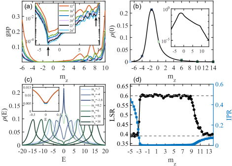
Figure 3: (Color online) (a) The gap versus $m_{z}$ for different system sizes calculated via the Lanczos method with the inset plotting the same thing in the logarithmic scale. The arrows show the universal dips. (b) The density of states (DOS) at zero energy $\rho(0)$ as a function of $m_{z}$ (with the logarithmic scale figure shown in the inset) calculated by the kernel polynomial method (KPM) for $L=55$ and $N_{c}=2^{11}$. (c) The DOS $\rho(E)$ versus $E$ for various $m_{z}$ in different phases for $L=55$ and $N_{c}=2^{11}$. The inset plots $\rho(E)$ versus $E$ when $m_{z}=6$ for $L=55$, $N_{c}=2^{11}$ (red line), $L=60$, $N_{c}=2^{11}$ (green line), and $L=60$, $N_{c}=2^{13}$ (blue line). (d) The level spacing ratio (LSR) $r(E=0)$ (left vertical axis) and inverse participation ratio (IPR) $I(E=0)$ (right vertical axis) for $L=24$ for the states around zero energy (only the states with negative energy are considered) computed via the Lanczos algorithm. In all above figures, samples in a cubic box are considered.

In Fig. 2(a), we show the Hall conductivity in comparison to the Bott index. We notice the clear consistence between them in a wide range of $m_{z}$ in an amorphous system as we expected. For the slight discrepancy, we estimate that it is caused by finite size effects of the Bott index, which exhibits conspicuous variations for distinct system sizes; the Hall conductivity does not show clear finite size effects when $L=24$ as their difference from $L=22$ is small (we consider a cubic case, $L_{x}=L_{y}=L_{z}=L$). Further, the Hall conductivity does not exhibit clear plateaus from finite size effects probably due to the smearing out around the gap closing region as in Weyl semimetals. The nonzero Hall conductivity and Bott index suggest the existence of a topological amorphous phase in a wide range of parameters.

To further identify the topological feature of the system, we calculate the local DOS defined as $\rho(E,{\bf x})=[\sum_{i}\delta(E-E_{i})(|\Psi_{E_{i},\uparrow\bf x}|^{2}+|\Psi_{E_{i},\downarrow\bf x}|^{2})]$, where $E_{i}$ is the $i$th eigenvalue, $\Psi_{E_{i},\sigma\bf x}$ with $\sigma=\uparrow,\downarrow$ are the corresponding components of the eigenstate of the system, and $[\cdots]$ denotes the average over samples. The DOS is defined as $\rho(E)=\sum_{\bf x}\rho(E,{\bf x})/(2N)$, which is normalized to one, i.e., $\int dE\rho(E)=1$. In Fig. 2(c) and (d), we illustrate the local DOS summed over $x_{z}$: $\sum_{x_{z}}\rho(E,{\bf x})$ for a system $L_{x}=L_{y}=20$ and $L_{z}=10$ for two typical values of $m_{z}$, clearly showing the presence of the surface states localized on the boundaries Supplement .

Band properties.— To discriminate the metal or semimetal phase from the insulator phase with respect to $m_{z}$, we compute the gap, twice of the lowest positive energy, using the Lanczos algorithm, and the DOS for large systems using the kernel polynomial method (KPM), which expands the DOS in Chebyshev polynomials to the order $N_{c}$ Alexander2006RMP .

Figure 3(a) and (b) illustrate the gap and the DOS at zero energy $\rho(E=0)$ with respect to the mass $m_{z}$ for distinct system sizes. Clearly, we see that the region with nonzero Bott index from $-2.8\lesssim m_{z}\lesssim 9$ corresponds to the gapless region: The gap for $-3.2<m_{z}<2$ is very small even for a small system size (see the red line for $L=16$) associated with a relative large DOS. $\rho(E=0)$ reaches the maximum at $m_{z}=-1.6$, where $\rho(E)$ versus $E$ exhibits a steep peak at zero energy as shown in Fig. 3(c), and it decreases sharply as $m_{z}$ moves away from this point associated with a developed minimum around zero energy for $\rho(E)$ (see Fig. 3(c)). When $2\lesssim m_{z}\lesssim 9$, while the energy gap strongly depends on the system size, its overall decline with increasing the system size can be observed, suggesting that this phase may be a semimetal or metal. Figure 3(b) further shows that $\rho(E=0)$ does not vanish in this region despite being small, implying that they correspond to a metal phase instead of a semimetal one. Specifically, for $m_{z}=6$, $\rho(E)$ shows a sudden drop around zero energy (see Fig. 3(c)), but this minimum does not vanish. To exclude the finite size effect, we calculate $\rho(E)$ using larger system size and $N_{c}$ and do not find conspicuous decline of $\rho(E=0)$ as shown in the inset of Fig. 3(c) Supplement , in stark contrast to a dramatic drop in a Weyl semimetal with quasiperiodic disorder Pixley2018PRL .

Viewing Fig. 3(a) in the logarithmic system (see the inset), we clearly see that there appears a universal dip of the energy gap for different system sizes at $m_{z}=9$ and $m_{z}=-2.8$. For the former, $\rho(E=0)$ exhibits a rapid decline to zero as $m_{z}$ increases from this point (see the inset in Fig. 3(b)), suggesting a phase transition to a band insulator [see $\rho(E)$ versus $E$ for $m_{z}=10,14$ in Fig. 3(c)]. More interestingly, for the latter, the DOS does not vanish and does not show clear nonanalytic behavior with respect to $m_{z}$. This phase is actually the Anderson localized insulator (dubbed amorphous Anderson insulator), which will be identified by the level-spacing statistics, the inverse participation ratio (IPR), the conductivity and the Fano factor. We note that with the further decline of $m_{z}$, the system develops into a band insulator [see $\rho(E)$ versus $E$ for $m_{z}=-7$ in Fig. 3(c)], but we cannot identify the transition point since the DOS becomes very small.

For level statistics, we calculate the adjacent level-spacing ratio (LSR): $r(E)=[\frac{1}{N_{E}-2}\sum_{i}\text{min}(\delta_{i},\delta_{i+1})/\text{max}(\delta_{i},\delta_{i+1})]$, where $\delta_{i}=E_{i}-E_{i-1}$ with $E_{i}$ being the $i$th eigenenergy sorted in an ascending order and $\sum_{i}$ is the sum over an energy bin around the energy $E$ with $N_{E}$ being the energy levels counted. It is well known that for localized states, $r\approx 0.39$ Huse2007PRB associated with the Poisson statistics and for extended states, $r\approx 0.6$ corresponding to the Gaussian unitary ensemble (GUE) Rigol2014PRX . Another signature we use is the real space IPR: $I(E)=[\frac{1}{N_{E}}\sum_{i}\sum_{\bf x}(|\Psi_{E_{i},\uparrow\bf x}|^{2}+|\Psi_{E_{i},\downarrow\bf x}|^{2})^{2}]$, which measures how much a state around energy $E$ is spatially localized. For a completely extended state in an infinitely large system, it is zero; for a state localized in a single site, it is one.

Figure 3(d) shows that, in the topological metal regime, $r(E=0)$ is around $0.6$ and $I(E=0)$ is almost zero; when $m_{z}$ decreases from $-2.8$, $r(E=0)$ drops to around $0.39$ and $I(E=0)$ increases sharply, indicating the phase transition from the extended phase to the localized one. Interestingly, we also see a similar change of the LSR and the IPR around $m_{z}\sim 9$, implying that the states around zero energy are localized even though the DOS becomes very small Supplement .

Conductivity and Fano factor.— To study the quantum transport properties of the amorphous system, we numerically calculate the transmission matrix $tt^{\dagger}$ at zero energy by the nonequilibrium Green’s function method DattaBook ; Sun2007PRB and determine the zero-temperature conductance by the Landauer formula $G=(e^{2}/h)\text{Tr}(tt^{\dagger})$ DattaBook and the Fano factor $F=\text{Tr}[tt^{\dagger}(1-tt^{\dagger})]/\text{Tr}(tt^{\dagger})$ Beenakker1992PRB ; Bergholtz2014PRL , for a system connected to two ideal terminals for $z<0$ and $z>L_{z}$.

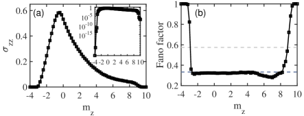
Figure 4: (Color online) Conductivity $\sigma_{zz}$ (a) in unit of $e^{2}/h$ and Fano factor (b) versus $m_{z}$ for $L=25$ in a cubic box. The inset plots the conductivity in the logarithmic scale, showing its steep drops across the phase transitions. The dashed lines correspond to $F=1/3$ and $F=1/3+1/(6\ln 2)$, respectively.

Figure 4(a) shows the conductivity $\sigma_{zz}=LG/W^{2}$ versus $m_{z}$ with $W$ and $L$ being the width and length of the system (we here consider a cubic box geometry, i.e., $W=L$ ). The conductivity is nonzero in the region with nonzero Bott index from $-2.8\lesssim m_{z}\lesssim 9$, showing a diffusive metal behavior as for a pseudoballistic semimetal the conductivity vanishes Bergholtz2014PRL . The conductivity drops to zero at around $m_{z}\sim-2.8$ and at around $m_{z}\sim 9$ when $m_{z}$ moves away to the left and right region, respectively. The former corresponds to the transition into the Anderson insulator phase, while the latter the band insulator phase with vanishing DOS. The diffusive metal behavior is also reflected in the Fano factor that takes the value around $F=1/3$ Beenakker1992PRB (see Fig. 4(b)). The transition into the insulator phase is signalled by the steep rise of the Fano factor to one due to the Poisson process. We do not find any discernible region where the Fano factor takes the value of $F_{0}=1/3+1/(6\ln 2)$ for Weyl semimetals without disorder Bergholtz2014PRL , further suggesting the absence of the semimetal phase Supplement .

Experimental realization.— Topological amorphous metals may be realized in classical systems, artificial quantum systems and solid-state glass materials. Here, we propose an experimental scheme to engineer a Laplacian (acting as a Hamiltonian) with electric circuits, which takes the form of our Hamiltonian Supplement . The surface states can be observed by measuring the two-point impedance. Recently, a number of topological phases, such as the SSH model Thomale2018CP , Weyl semimetals Simon2019PRB and higher topological insulators Thomale2018NP have been experimentally observed with electric circuits. In addition, recent development of technology has allowed us to place Rydberg atoms in arbitrary geometry using optical tweezers Browaeys2016Science ; Lukin2016Science , which makes it possible to realize our model in this system.

In summary, we have discovered a topological amorphous metal phase in 3D amorphous systems. We identify its topological feature by calculating the Bott index, the Hall conductivity and the surface states. Through further studying its band properties including the energy gap, DOS, LSR and IPR and the quantum transport properties, we find that the topological phase exhibits a diffusive metal behavior. We further predict the phase transition from the topological metal phase to the Anderson insulator phase and the band insulator phase with respect to a system parameter. Our results open a new avenue for studying topological gapless phenomena in amorphous systems. These new phenomena might be observed in various amorphous materials, such as engineered classical or atomic systems and glass materials.

I Supplemental Material

In the supplementary material, we will prove the equivalence between the generalized Bott index and the Hall conductivity in 3D Weyl semimetals in Section 1, show the Griffiths effects in Section 2 and the density profiles of the surface states in Section 3, give more discussion on the semimetal phase in Section 4, illustrate the mobility edge in distinct phases in Section 5 and the effects of $R_{c}$ and the on-site disorder in Section 6, and finally introduce an experimental scheme with electric circuits in Section 7.

II S-1. Proof for the equivalence between the Bott index and the Hall conductivity

In this section, we will prove the equivalence between the Bott index defined in the main text and the Hall conductivity in 3D Weyl semimetals with translational symmetry, following the method used to prove its equivalence to the Chern number in 2D systems Rigol2017PRA . For a Weyl semimetal, let us define the Bott index as

$$\mathrm{Bott}_{3}=\frac{1}{2\pi L_{3}}\text{Im}\text{Tr}\log(U),$$ (S1)

where $U=\tilde{U}_{2}\tilde{U}_{1}\tilde{U}_{2}^{\dagger}\tilde{U}_{1}^{\dagger}$, $U_{i}=Pe^{2\pi i\hat{{\bf r}}\cdot{\bf a}_{i}/(L_{i}a_{i})}P=\left(\begin{array}[]{cc}0&0\\ 0&\tilde{U}_{i}\\ \end{array}\right)$ with the position operator $\hat{\bf r}=\sum_{i=1,2,3}\hat{x}_{i}{\bf a}_{i}$, ${\bf a}_{i}$ being the lattice vectors and $L_{i}$ being the size of the system along the ${\bf a}_{i}$ direction; $\tilde{U}_{i}$ is the reduced matrix in the occupied space and $P$ is the projection operator that projects states into the occupied space. In a system with translational symmetry, $P$ can be expressed as $P=\sum_{n{\bf k}}|n{\bf k}\rangle\langle n{\bf k}|$ where $|n{\bf k}\rangle$ denotes the occupied Bloch state in the $n$th band with the quasimomentum ${\bf k}=\sum_{i=1,2,3}k_{i}{\bf G}_{i}/(2\pi)$, where ${\bf G}_{i}$ is the reciprocal lattice vector. In the coordinate representation, the Bloch state takes the form of $\langle{\bf r}|n,{\bf k}\rangle=e^{i{\bf k}\cdot{\bf r}}u_{n,{\bf k}}({\bf r})=e^{i{\bf k}\cdot{\bf r}}\langle{\bf r}|u_{n,{\bf k}}\rangle$ where $u_{n,{\bf k}}({\bf r+{\bf a}_{i}})=u_{n,{\bf k}}({\bf r})$. In this basis, we can expand $U$ in terms of $\delta k_{i}$ with $\delta k_{i}=2\pi a_{i}/L_{i}$ ($i=1,2$),

$$U= \sum_{n_{1},n_{2},...,n_{5}}\sum_{{\bf k}}|n_{1},{\bf k}\rangle\langle u_{n_{1},{\bf k}}|u_{n_{2},k_{1},k_{2}-\delta k_{2},k_{3}}\rangle\langle u_{n_{2},k_{1},k_{2}-\delta k_{2},k_{3}}|u_{n_{3},k_{1}-\delta k_{1},k_{2}-\delta k_{2},k_{3}}\rangle$$ (S2)

$$\langle u_{n_{3},k_{1}-\delta k_{1},k_{2}-\delta k_{2},k_{3}}|u_{n_{4},k_{1}-\delta k_{1},k_{2},k_{3}}\rangle\langle u_{n_{4},k_{1}-\delta k_{1},k_{2},k_{3}}|u_{n_{5},{\bf k}}\rangle\langle n_{5},{\bf k}|$$

$$= U_{0}+U_{2}+O(\delta k^{3}),$$ (S3)

where

$$U_{0} = \sum_{n}\sum_{\bf k}|n\rangle\langle n|,$$ (S4)

$$U_{2} = \sum_{n_{1},n_{2}}\sum_{\bf k}|n_{1}\rangle\langle n_{2}|\big{[}\delta k_{1}\delta k_{2}\big{(}(\partial_{k_{2}}\langle u_{n_{1}}|)(\partial_{k_{1}}|u_{n_{2}}\rangle)-k_{1}\leftrightarrow k_{2}\big{)}\big{.}$$ (S5)

$$\big{.}+\frac{1}{2}\sum_{i=1,2}\delta k_{i}^{2}(\langle u_{n_{1}}|\partial^{2}_{k_{i}}u_{n_{2}}\rangle+\langle\partial^{2}_{k_{i}}u_{n_{1}}|u_{n_{2}}\rangle)\big{]}$$

$$+\sum_{n_{1},n_{2},n_{3}}\sum_{\bf k}|n_{1}\rangle\langle n_{3}|\big{[}\sum_{i=1,2}\delta k_{i}^{2}\langle u_{n_{1}}|\partial_{k_{i}}u_{n_{2}}\rangle\langle\partial_{k_{i}}u_{n_{2}}|u_{n_{3}}\rangle$$

$$+\delta k_{1}\delta k_{2}\langle u_{n_{1}}|\partial_{k_{1}}u_{n_{2}}\rangle\langle\partial_{k_{2}}u_{n_{2}}|u_{n_{3}}\rangle+\delta k_{1}\delta k_{2}\langle\partial_{k_{2}}u_{n_{1}}|u_{n_{2}}\rangle\langle\partial_{k_{1}}u_{n_{2}}|u_{n_{3}}\rangle\big{]},$$

where $n_{i}$ denotes the occupied bands, and, for briefness, we have skipped the index for ${\bf k}$. Let us further decompose $U$ into $U=1+U_{\bar{D}}+U_{O}$ where $U_{\bar{D}}+1$ denotes the diagonal part and $U_{O}$ the off-diagonal one. Using this decomposition, we obtain

$$\text{Tr}\log U=\text{Tr}U_{\bar{D}}-\frac{1}{2}\text{Tr}(U_{\bar{D}}+U_{O})^{2}+O((U_{\bar{D}}+U_{O})^{3}).$$ (S6)

Since $U_{\bar{D}}+U_{O}$ is at least the second order of $\delta k$, the second term contributes a fourth order term and hence we neglect it. To the second order, we only need to evaluate the diagonal part, which is

$$\text{Tr}U_{\bar{D}}=\text{Tr}U_{2} = \sum_{n}\sum_{\bf k}\big{[}\delta k_{1}\delta k_{2}\big{(}\langle\partial_{k_{2}}u_{n}|\partial_{k_{1}}u_{n}\rangle-k_{1}\leftrightarrow k_{2}\big{)}+\frac{1}{2}(\sum_{i=1,2}\delta k_{i}^{2}\langle u_{n}|\partial^{2}_{k_{i}}|u_{n}\rangle+c.c.)\big{]}$$ (S7)

$$+\sum_{n}\sum_{\bf k}\sum_{n^{\prime}}\sum_{i=1,2}\delta k_{i}^{2}|\langle u_{n}|\partial_{k_{i}}u_{n^{\prime}}\rangle|^{2},$$

where only the first term contributes to the Bott index as all other terms are purely real. Therefore, to the second order, we have

$$\mathrm{Bott}_{3} = \frac{1}{2\pi L_{3}}\sum_{n}\sum_{\bf k}\delta k_{1}\delta k_{2}\Omega_{3}({\bf k})$$ (S8)

$$= \frac{1}{2\pi}\sum_{n}\int_{0}^{2\pi}dk_{3}C_{n}(k_{3}),$$ (S9)

where $\Omega_{3}({\bf k})=i(\langle\partial_{k_{1}}u_{n}|\partial_{k_{2}}u_{n}\rangle-k_{1}\leftrightarrow k_{2})$ is the Berry curvature along the ${\bf G}_{3}$ direction and $C_{n}$ is the Chern number for a fixed $k_{3}$ in the $n$th occupied band. Evidently, this is the Hall conductivity $\sigma_{12}$ in unit of $e^{2}/h$ and hence we prove the equivalence between the Bott index and the Hall conductivity in a Weyl semimetal.

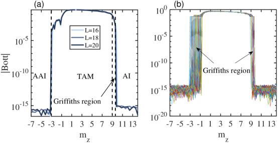
Figure S1: (Color online) The absolute value of the averaged Bott index (a) and the Bott index for 181 samples for $L=20$ (b) with respect to $m_{z}$ in the logarithmic scale.

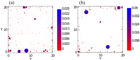
Figure S2: (Color online) Top view of the surface states for two typical states for $m_{z}=2$ (a) and $m_{z}=6$ (b). Here, the color and the size of circles depict the profile of the surface states, which are clearly localized around the boundaries.

III S-2. Griffiths region

In Fig. S1, we plot the absolute value of the Bott index in the logarithmic scale, which clearly shows that the Bott index drops to zero across the phase boundaries. We have also noticed that, in the region $9<m_{z}<9.6$, while the system transitions into an insulating phase, the Bott index does not vanish despite being small. To interpret such phenomena, we plot the absolute value of the Bott index for all 181 samples in Fig. S1(b), illustrating that, in this region, some samples have nonzero Bott index while others have zero, suggesting that this region corresponds to a Griffiths region.

IV S-3. Surface states

In the main text, we show the local DOS in a flat-box like geometry with the height much shorter than the other two dimensions (here we take $L_{x}=L_{y}=20$ and $L_{z}=10$). Here, we use the same geometry so that the system is gapped under periodic boundary conditions. This enables us to pick up the surface states that are located inside the gap under open boundary conditions along the x and y directions. We illustrate the top view of the surface states in Fig. S2(a) and (b), clearly showing their localization on the boundaries. The IPR of the two states are 0.0027 and 0.0066, respectively, which are in the same order of $1/(4L_{x}L_{z})=0.0013$, the IPR for a state uniformly distributed on the surfaces.

V S-4. Discussion on semimetal phases

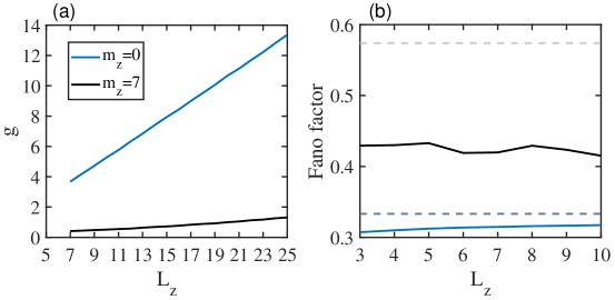
Figure S3: (Color online) (a) $g$ versus $L_{z}$ for $L_{x}=L_{y}=25$ and (b) the Fano factor versus $L_{z}$ for $L_{x}=L_{y}=40$.

To further verify the absence of the semimetal phase, let us study the intrinsic conductivity and the Fano factor in a flat-box geometry. By defining a dimensionless parameter

$$g=G\frac{h}{e^{2}}\frac{L_{z}^{2}}{W^{2}},$$ (S10)

we write the intrinsic conductivity (eliminating the contact resistance contribution) as

$$\sigma_{I}=\frac{1}{W^{2}\partial R/\partial L_{z}}=\frac{e^{2}}{h}\frac{1}{\partial(L_{z}^{2}/g)/\partial L_{z}},$$ (S11)

where $R=1/G=\frac{L_{z}^{2}}{W^{2}g}\frac{h}{e^{2}}$ is the resistance. For a diffusive metal, $g\propto L_{z}$ as $L_{z}\rightarrow\infty$ so that $\sigma_{I}$ is finite, while in a pseudo-ballistic regime corresponding to a semimetal, $g$ has an upper bound as $L_{z}\rightarrow\infty$ so that $\sigma_{I}$ goes zero. In Fig. S3(a), we see that for both $m_{z}=0$ and $m_{z}=7$, $g$ increases with $L_{z}$ with a linear scaling, suggesting that the $\sigma_{I}$ do not vanish in both cases, while the slope is much smaller for $m_{z}=7$. In Fig. S3(b), we further plot the Fano factor using a flat-box like geometry with $W=40$ as a function of $L_{z}$, illustrating that the Fano factor is slightly below $1/3$ for $m_{z}=0$ and increases slowly with increasing $L_{z}$, while for $m_{z}=7$, the value stays around $0.43$, which is between the value (0.5738) for a semimetal and $1/3$ for a metal. As the geometry becomes a cubic, the Fano factor for $m_{z}=0$ goes to $1/3$ while for $m_{z}=7$ goes below $1/3$ (see Fig. 4(b) in the main text).

VI S-5. Mobility edges

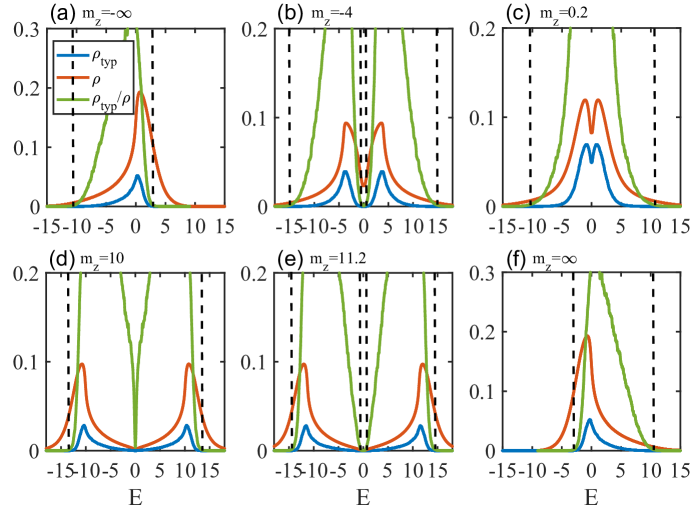
Figure S4: (Color online) The typical DOS, the DOS and their ratio versus $E$ for different values of $m_{z}$. In (a) and (f) where $|m_{z}|\rightarrow\infty$, the constant energy $m_{z}$ is not included and only the lower band information is plotted. The dashed black lines denote the mobility edge. Here, the DOS and the typical DOS are numerically calculated with $L=55$, $N_{c}=2^{11}$, and $L=55$, $N_{c}=2^{12}$ in a cubic box, respectively.

In this section, we study the mobility edge in our system where the system transitions into the extended phase from the localized one as the Fermi surface is tuned. For clarity, let us first consider the limit that $m_{z}\rightarrow-\infty$. Based on the perturbation theory to the first order, we obtain the following effective Hamiltonian

$$H_{eff}=\sum_{\bf x}\left[\sum_{\bf R}t(R)\hat{c}^{\dagger}_{{\bf x},\uparrow}\hat{c}_{{\bf x}+{\bf R},\uparrow}+m_{z}\hat{c}^{\dagger}_{{\bf x},\uparrow}\hat{c}_{{\bf x},\uparrow}\right],$$ (S12)

which describes a spinless particle in a 3D amorphous system. In Fig. S4(a), we plot the DOS of this system without including the constant term $m_{z}$. The DOS is asymmetric with respect to $E$. For a cubic lattice configuration, it shares the asymmetric characteristic due to the presence of the long-range hopping, in stark contrast to the case with only the nearest-neighbor hopping.

To determine the mobility edge, we calculate the typical DOS defined as

$$\rho_{typ}(E)=e^{[\frac{1}{N}\sum_{{\bf x}}\text{log}\rho(E,{\bf x})]},$$ (S13)

where $[\cdots]$ indicates the average over distinct samples. The typical DOS is numerically calculated by the KPM. When the DOS is finite, the vanishing of the typical DOS reflects the appearance of localized states. In Fig. S4, we display both the DOS and typical DOS in different phases. For $m_{z}=\pm\infty$, it is evident to see that there exist regions around the band edges where the typical DOS vanishes while the DOS is still finite, showing the localized characteristic in these regions; Yet, in other regions, both the typical DOS and the DOS are finite, showing their extended feature. This demonstrates the existence of the mobility edge where $\rho_{typ}/\rho$ vanishes. We also observe that the localized phase is more conspicuous for the positive $E$ than the negative one, where the DOS is very small. This explains the clear presence of the AAI for the negative $m_{z}$, but not for the positive one. Now let us raise $m_{z}$ to $-4$, we observe that there still exists a small region around zero and a region around other band edges which correspond to a localized phase. As we increase $m_{z}$ further, the localized phase for the former disappears while that for the latter persists. When $m_{z}\rightarrow\infty$, both the DOS and the typical DOS are antisymmetric to the case when $m_{z}\rightarrow-\infty$. As we decrease $m_{z}$ to $11.2$ and further to $10$, both the DOS and typical DOS are very small. While the phase corresponds to a band insulator, the states around zero energy are localized (which is also reflected by the LSR and IPR) despite the region being very small.

VII S-6. Effects of $R_{c}$ and stability against the on-site disorder

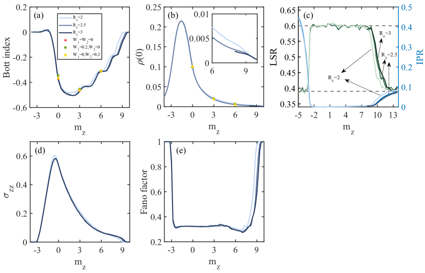
Figure S5: (Color online) The Bott index for $L=16$ (a), the DOS at zero energy for $L=55$ and $N_{c}=2^{11}$ (b), the LSR and the IPR for $L=24$ (c), the longitudinal conductivity (d) and the Fano factor (e) with respect to $m_{z}$ for three distinct $R_{c}$. In (a), the red stars, green circles and yellow diamonds show the Hall conductivity for the disorder strength $W_{1}=W_{2}=0$, $W_{1}=0.2,W_{2}=0$, and $W_{1}=0,W_{2}=0.2$ respectively. In (b), the green circles and yellow diamonds show the DOS at zero energy for $W_{1}=0.2,W_{2}=0$ and $W_{1}=0,W_{2}=0.2$, respectively, and the inset shows the zoomed-in view of the DOS. In (d) and (e), the light and dark blue lines correspond to $L=24$ while the other one $L=25$. Here, all samples are considered in a cubic box.

In this section, we discuss the effects of $R_{c}$ and the on-site disorder on our results. In Fig. S5, we plot the Bott index, the DOS at zero energy, the LSR and the IPR, the longitudinal conductivity $\sigma_{zz}$ and the Fano factor for $R_{c}=2,2.5,3$. It clearly shows that $R_{c}$ has only quantitative effects on our results: increasing $R_{c}$ from $2$ to $3$ only slightly shifts the phase boundary on the right side, while has vanishing effects on the phase boundary on the left side. We note that the shift between $R_{c}=2.5$ and $3$ is very small.

To verify that our results are stable against the on-site disorder, we calculate the Hall conductivity and the DOS at zero energy in the presence of the following term

$$H_{D}=\sum_{\bf x}\hat{c}_{\bf x}^{\dagger}[W_{1}V_{1}({\bf x})+W_{2}V_{2}({\bf x})\sigma_{z}]\hat{c}_{\bf x},$$ (S14)

where $V_{1}({\bf x})$ and $V_{2}({\bf x})$ are uniformly random variables chosen from $[-1,1]$. Fig. S5(a-b) illustrates that the presence of a weak disorder only has a very slight modification of the Hall conductivity and the DOS, suggesting stability of our results against the on-site disorder.

VIII S-7. Experimental realization in electric circuits

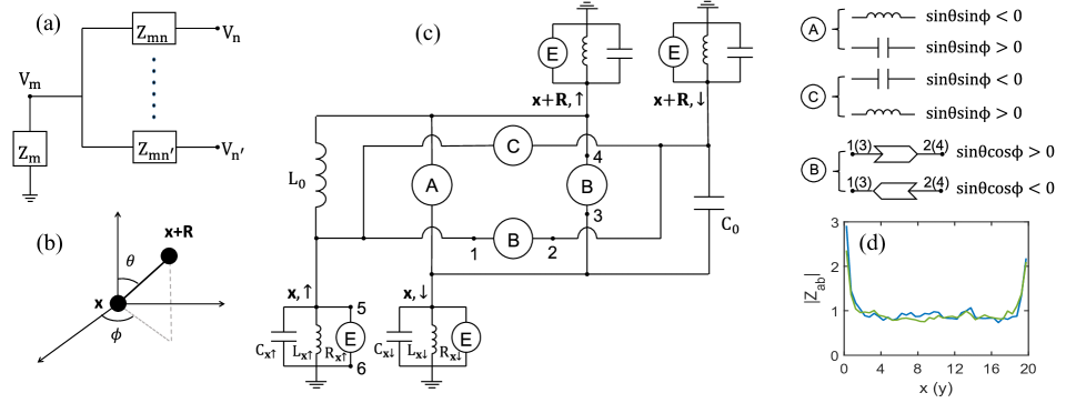
Figure S6: (Color online) (a) Schematics of a simple electrical network. Electric circuits (c) between four nodes (with spins) located at $\bf x$ and ${\bf x}+{\bf R}$ as shown in (b). $C_{0}$, $C_{{\bf x}\sigma}$, $L_{0}$, and $L_{{\bf x}\sigma}$ denote the corresponding capacitances and inductances. The labeled circles represent electrical elements which depend on the geometry between two nodes. For the circle labelled by B, it represents a negative impedance converter with current inversion (INIC) Thomale2018arX ; ChenBook , the sign of the resistance depends on how the INIC is connected. For instance, if $\sin\theta\cos\phi>0$, we require that the direction of the INIC is from point 1 to point 2, so that $I_{12}=-(V_{1}-V_{2})/|R_{B}|$ corresponding to the negative resistance while $I_{21}=(V_{2}-V_{1})/|R_{B}|$ corresponding to the positive resistance. The electric element labelled by $E$ also depicts the INIC with the corresponding resistance $R_{{\bf x}\sigma}$, the sign of which is dependent of the orientation of the INIC. (d) The averaged two-node impedance versus the coordinate of each divided layer for $m_{z}=2$. For the blue (green) line, we divide the system into 40 layers perpendicular to the $x$ ($y$) direction and each pair of nodes are chosen randomly in each layer. The unit of the impedance is $\omega\bar{L}_{0}$.

In this section, we introduce a scheme (shown in Fig. S6) to implement our Hamiltonian in electric circuits. Let us consider an electrical network where the current flowing from node $m$ to node $n$ is denoted by $I_{mn}$ and the electric potential at each node $m$ is denoted by $V_{m}$. According to Kirchhoff’s law,

$$I_{m}=\sum_{n}I_{mn}=\sum_{n}Y_{mn}(V_{m}-V_{n})+Y_{m}V_{m},$$ (S15)

where $Y_{mn}=1/Z_{mn}$ is the admittance between node $m$ and $n$ with $Z_{mn}$ being the corresponding impedance and $Y_{m}=1/Z_{m}$ is the admittance between node $m$ and the ground as shown in Fig. S6(a). We can write this equation in a matrix form

$$I=JV,$$ (S16)

where $I=(\begin{array}[]{cccc}I_{1}&I_{2}&\cdots&I_{M}\end{array})^{T}$ and $V=(\begin{array}[]{cccc}V_{1}&V_{2}&\cdots&V_{M}\end{array})^{T}$ with $M$ labelling the total number of nodes. Here, $J$ is the Laplacian acting as the Hamiltonian that can be used to simulate our system. We note that such methods have been used to probe the SSH model Thomale2018CP , Weyl semimetals Simon2019PRB and higher topological insulators Thomale2018NP .

To implement our Hamiltonian, let us write the Hamiltonian as

$$H=\sum_{({\bf x},{\bf x}+{\bf R})}H({\bf x},{\bf x}+{\bf R})+\sum_{\bf x}H({\bf x}),$$ (S17)

where $H({\bf x},{\bf x}+{\bf R})$ depicts the hopping between two neighbor sites ${\bf x}$ and ${\bf x}+{\bf R}$ and $H({\bf x})$ the on-site term. We only need to construct the hopping between two sites and the on-site term and all other connections can be built in a similar way. We propose an electric circuit shown in Fig. S6(c) which can be described by

$$J=i\omega[\mathcal{J}({\bf x},{\bf x}+{\bf R})+\mathcal{J}_{0}({\bf x},{\bf R})+\mathcal{J}({\bf x})],$$ (S18)

where

$$\mathcal{J}({\bf x},{\bf x}+{\bf R})= -C_{0}(R)\left[|\pi_{{\bf x},\uparrow}\rangle\langle\pi_{{\bf x}+{\bf R},\uparrow}|-|\pi_{{\bf x},\downarrow}\rangle\langle\pi_{{\bf x}+{\bf R},\downarrow}|+(i\sin\theta\cos\phi+\sin\theta\sin\phi)|\pi_{{\bf x}\uparrow}\rangle\langle\pi_{{\bf x}+{\bf R},\downarrow}|\right.$$ (S19)

$$\left.+(i\sin\theta\cos\phi-\sin\theta\sin\phi)|\pi_{{\bf x},\downarrow}\rangle\langle\pi_{{\bf x}+{\bf R},\uparrow}|+H.c.\right]$$

$$\mathcal{J}_{0}({\bf x},{\bf R})= -C_{0}(R)(1-\sin\theta\sin\phi-i\sin\theta\cos\phi)|\pi_{{\bf x},\uparrow}\rangle\langle\pi_{{\bf x},\uparrow}|$$ (S20)

$$-C_{0}(R)(-1+\sin\theta\sin\phi-i\sin\theta\cos\phi)|\pi_{{\bf x},\downarrow}\rangle\langle\pi_{{\bf x},\downarrow}|$$

$$\mathcal{J}({\bf x})= \sum_{\sigma=\uparrow,\downarrow}(C_{{\bf x},\sigma}-\frac{1}{\omega^{2}L_{{\bf x},\sigma}}-i\frac{1}{\omega R_{{\bf x},\sigma}})|\pi_{{\bf x},\sigma}\rangle\langle\pi_{{\bf x},\sigma}|,$$ (S21)

and $|\pi_{{\bf x},\uparrow}\rangle$ depicts a row vector with an entry corresponding to the node ${\bm{\xi}}=({\bf x},\sigma)$ being one and all other entries being zero, and $C_{0}(R)=1/(\omega^{2}L_{0})=e^{\lambda(1-R)}/(2\omega^{2}\bar{L}_{0})$ with $\omega$ being the frequency of the alternating current. For the whole system, the contribution from $\mathcal{J}_{0}({\bf x},{\bf R})$ should be summed over ${\bf R}$. By appropriately tuning the circuit elements so that $R_{{\bf x},\uparrow}=R_{{\bf x},\downarrow}=1/(\omega\sum_{\bf R}C_{0}(R)\sin\theta\cos\phi)$, $C_{{\bf x}\uparrow}=1/(\omega^{2}L_{{\bf x}\downarrow})$, $C_{{\bf x}\downarrow}=1/(\omega^{2}L_{{\bf x}\uparrow})$ and $C_{{\bf x},\uparrow}-C_{{\bf x},\downarrow}=m_{z}/(\omega^{2}\bar{L}_{0})+\sum_{\bf R}C_{0}(R)(1-\sin\theta\sin\phi)$, we achieve the expected Laplacian $J=iH/(\omega\bar{L}_{0})$. To measure the surface states, we divide the system into a number of layers and measure the impedance between two nodes in each layer. The averaged impedance is given by

$$|Z_{ab}|=[|\sum_{n}\frac{|\Psi_{E_{n},{\bm{\xi}}_{a}}-\Psi_{E_{n},{\bm{\xi}}_{b}}|^{2}}{j_{n}}|],$$ (S22)

where $[\cdots]$ indicates the average over different pairs of two nodes and different samples and $\Psi_{E_{n},{\bm{\xi}}_{a}}$ is the ${\bm{\xi}}_{a}$ component of the eigenvector of $J$ corresponding to the eigenvalue $j_{n}$. Figure S6 plots the impedance in different layers, showing that the impedance exhibits peaks around the boundaries, suggesting the presence of the surface states.

References

- (1) Y. Ge and M. Rigo, Phys. Rev. A 96, 023610 (2017).
- (2) C. H. Lee, S. Imhof, C. Berger, F. Bayer, J. Brehm, L. W. Molenkamp, T. Kiessling, and R. Thomale, Commun. Phys. 1, 39 (2018).
- (3) Y. Lu, N. Jia, L. Su, C. Owens, G. Juzeliunas, D. I. Schuster, and J. Simon, Phys. Rev. B 99, 020302(R) (2019).
- (4) S. Imhof, C. Berger, F. Bayer, J. Brehm, L. W. Molenkamp, T. Kiessling, F. Schindler, C. H. Lee, M. Greiter,T. Neupert, and R. Thomale, Nat. Phys. 14, 925 (2018).
- (5) T. Hofmann, T. Helbig, C. H. Lee, M. Greiter, and R. Thomale, arXiv:1809.08687 (2018).
- (6) W.-K. Chen, The Circuits and Filters Handbook, 3rd ed. (CRC Press, Inc., Boca Raton, FL, USA, 2009).