Geometrically Frustrated Anisotropic Four-Leg Spin-1/2 Nanotube

Abstract

We develop a real space quantum renormalization group (QRG) to explore a frustrated anisotropic four-leg spin-1/2 nanotube in the thermodynamic limit. We obtain the phase diagram, fixed points, critical points, the scaling of coupling constants and magnetization curves. Our investigation points out that in the case of strong leg coupling the diagonal frustrating interaction is marginal under QRG transformations and does not affect the universality class of the model. Remarkably, the renormalization equations express that the spin nanotube prepared in the strong leg coupling case goes to the strong plaquette coupling limit (weakly interacting plaquettes). Subsequently, in the limit of weakly interacting plaquettes, the model is mapped onto a 1D spin-1/2 XXZ chain in a longitudinal magnetic field under QRG transformation. Furthermore, the effective Hamiltonian of the spin nanotube inspires both first and second order phase transitions accompanied by the fractional magnetization plateaus. Our results show that the anisotropy changes the magnetization curve and the phase transition points, significantly. Finally, we report the numerical exact diagonalization results to compare the ground state phase diagram with our analytical visions.

I Introduction

The induces non-trivial magnetic states are currently renewed interest in the magnetic quantum spin systems that exhibit a geometrical frustration Claudine et al. (2011); Hung (2013). These states are fascinating because of their intriguing and unique properties compare to conventional magnetic systems, e.g., unconventional magnetic orders or even a disorder Claudine et al. (2011); Hung (2013); Jafari and Langari (2007). They have attracted more attention by experimental realization of $J_{1}-J_{2}$ chain Hase et al. (1993), whereas a geometric frustrated spin can be advanced to a family of problems concerns the integer-spin ladders Cabra et al. (1998); Dagotto and Rice (1996); Dagotto (1999). A nice extension of two-leg spin ladders have been performed for the various quantum $n$-leg spin ladder, which are recognized as tubelike lattice structures for $n\geq 3$ Uehara et al. (1996); Cabra et al. (1998); Charrier et al. (2010). Therewith, according to the Lieb-Schultz-Mattis theorem, their ground state can be either gapped with a broken translational invariance, or gapless (non-degenerate) Lieb et al. (1961); Arlego et al. (2013).

An illustrative example is a triangular frustrated structure, which can be found in the three-leg spin tubes with the larger frustration and quantum fluctuations Kawano and Takahashi (1997); Wang (2001). These three-leg spin tubes have been studied intensively both experimentally and theoretically Kawano and Takahashi (1997); Wang (2001); Sato and Sakai (2007); Lüscher et al. (2004); Sato (2007); Sakai et al. (2008); Manaka et al. (2011); Hagihala et al. (2019); Ochiai et al. (2017); Seki and Okunishi (2015), and have been developed by synthesizing of odd number ($n$) of the legs spin tube, such as [(CuCl₂tachH)₃Cl]Cl₂ Schnack et al. (2004), and XCrF₄ (X=Cs or K) with $n=3$ Manaka et al. (2009), as well as, Na₂V₃O₇ with $n=9$ Millet et al. (1999). One of the most recent example is a four-leg spin-1/2 nanotube Cu₂Cl₄·D₈C₄SO₂ with next-nearest neighbor (NNN) AFM interaction, and diagonally coupling adjacent legs (Fig. 1) Garlea et al. (2008); Zheludev et al. (2008); Garlea et al. (2009). Although, the spin tubes with an odd number of legs and only nearest neighbor antiferromagnetic (AFM) intrachain coupling are geometrically frustrated, it is well known that the four-leg spin tube with only nearest neighbor AFM exchange is not frustrated, neither in the weak or the strong plaquette coupling limits Arlego et al. (2013); Arlego and Brenig (2011); Cabra et al. (1997, 1998); Totsuka (1997); Kim and Sólyom (1999).

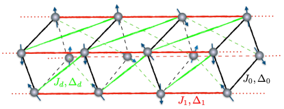
Figure 1: (Color online) Schematic representation of the frustrated four-leg spin tube. The interaction along the legs is characterized by $J_{1}$ (red lines), $J_{0}$ shows the intra-plaquettes infraction (black lines), and the diagonal interaction $J_{d}$ has been shown by the green lines.

The frustration in four-leg spin tube arrises by considering the next nearest coupling or diagonal interaction (see $J_{d}$, green lines, in Fig. 1). This has generated much recent interest, and there have been several theoretical attempts to look at the frustrated isotropic four-leg spin tube (FAFST) Arlego and Brenig (2011); Arlego et al. (2013); Gómez Albarracín et al. (2014); Rosales et al. (2014); Plat et al. (2015). In particular, it has been investigated using the density matrix renormalization group (DMRG)Gómez Albarracín et al. (2014), exact diagonalization, series expansionArlego and Brenig (2011), Schwinger bosons mean field theory, and quantum Monte-Carlo simulation Arlego et al. (2013). Moreover, a study of the phases of the FAFST in the presence of a magnetic field has been done in a combined analysis using perturbative methods, variational approach and DMRG Gómez Albarracín et al. (2014).

Although the magnetic properties of the FAFST model has been investigated in previous works, still the perceptive of the quantum phases on a larger scale is missing Arlego et al. (2013). In this light, it is inexplicable that the phase diagram is not fully understood, and also the universality class of the model is unknown in the presence of anisotropy. This encourages us to investigate the FAFST model in the presence of a magnetic field using the real space renormalization group (RSRG) approach.

In this respect, we demonstrate the ground state magnetic phase diagram of such a system, and aim to show that in the limit of the strong leg coupling the diagonal frustrating interaction does not flow under QRG transformation. Furthermore, in the limit of the strong leg coupling, the spin tube goes to the strong plaquette coupling limit (weakly interacting plaquettes) under renormalization transformations. Subsequently, in the strong plaquette coupling limit, under RSRG transformation, the FAFST model maps onto the one-dimensional (1D) spin-1/2 XXZ model in the presence of an effective magnetic field. We also show that when the leg and frustrating couplings are the same (maximum frustration line), only first order quantum phase transitions is observed at zero temperature. This results that the magnetization (per particle) process exhibits fractional plateaus at zero, one-quarter, one-half and three-quarter of the saturation magnetization. We find that away from the maximum frustration line the model exhibits both first and second order quantum phase transitions. In addition, the numerical Lanczos method is applied for the finite size spin-1/2 nanotubes and mentioned behavior is approved.

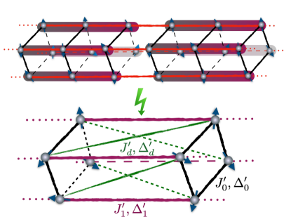
Figure 2: (Color online) Renormalization scheme of frustrated four-leg nano-spin tube in the strong leg-coupling limit, where a three site blocks Hamiltonian along the legs (top) are mapped to a renormalized spins (bottom).

II FAFST model: Real Space Renormalization Group Study

II.1 Theoretical Model

We consider the Hamiltonian of the geometrically frustrated anisotropic four-leg spin tube (FAFST) model in the presence of a magnetic field on a periodic tube of $N$ sites, which is given by

$$\begin{aligned} {\cal H}=\frac{1}{4}\sum_{i=1}^{N}\sum_{\alpha=1}^{4}\Big{[}&{\cal H}_{0}^{(i,\alpha;\;i,\alpha+1)}+{\cal H}_{1}^{(i,\alpha;\;i+1,\alpha)}\\ &+{\cal H}_{d}^{(i,\alpha;\;i+1,\alpha+1)}-2h\sigma^{z}_{i,\alpha}\Big{]}.\\ \end{aligned}$$ (1)

Here we define

$${\cal H}_{n}^{(i,\alpha;\;j,\beta)}=J_{n}(\sigma^{x}_{i,\alpha}\sigma^{x}_{j,\beta}+\sigma^{y}_{i,\alpha}\sigma^{y}_{j,\beta})+\Delta_{n}\sigma^{z}_{i,\alpha}\sigma^{z}_{j,\beta},$$ (2)

with $n=(0,1,\;d)$, the indeses $\alpha,\beta=1-4$ run over intra-plaquettes spins and $i,j$ count the inter-plaquettes sites. Here $J_{0}$, $J_{1}$ and $J_{d}$ are the plaquette, leg, and diagonal exchange couplings respectively, and the corresponding easy-axis anisotropies are defined by $\Delta_{0}$, $\Delta_{1}$ and $\Delta_{d}$. Furthermore, $\vec{\boldsymbol{\sigma}}=(\sigma^{x},\sigma^{y},\sigma^{z})$ denotes the Pauli matrices, and $h$ represents a magnetic field to point along the $z$-direction.

The FAFST model is invariant under several symmetry operations: one-site translation $\vec{{\boldsymbol{\sigma}}}_{i,\alpha}\rightarrow\vec{{\boldsymbol{\sigma}}}_{i+1,\alpha}$, bond-centered inversion $\vec{{\boldsymbol{\sigma}}}_{i,\alpha}\rightarrow\vec{{\boldsymbol{\sigma}}}_{1-i,\alpha}$, time reversal $\vec{{\boldsymbol{\sigma}}}_{i,\alpha}\rightarrow-\vec{{\boldsymbol{\sigma}}}_{i,\alpha}$, $U(1)$ spin rotation around the $z$ axis, and $\pi$ rotation around the $x$ or $y$ axis Fuji (2016). We should mention that the isotropic form of the above Hamiltonian, $\Delta_{n=0,1,d}=1$, has the $SU(2)$ symmetry in the absence of the magnetic field.

Based on real Space Renormalization group approach (Appendix A), and using the low-energy effective Hamiltonian we discuss the properties of the spin tube, Eq. (1) in two possible limits. The first limit that is considered in the section II.2, corresponds to the strong leg-coupling and is defined by $J_{1}/J_{0,d}\rightarrow\infty$. The second case, is the strong plaquette coupling limit $J_{0}/J_{1,d}\rightarrow\infty$ and is reviewed in the section II.3, which corresponds to almost decoupled plaquettes.

II.2 The strong leg coupling limit: $J_{1}/J_{0,d}\rightarrow\infty$

In this regime the spin nanotube resembles a chain of four weakly coupled XXZ chains where the weak plaquette coupling $J_{0}$ and diagonal coupling $J_{d}$ can be treated perturbatively. We study this limit for two different cases of in the absence and in the presence of external fields:

II.2.1 In the absence of the magnetic field: $h=0$

As a first step, to get a better understanding of the spin tube properties in the strong leg-coupling limit, we look at the Hamiltonian without the magnetic field, $h=0$. To implement the idea of QRG in the strong leg-coupling limit, we use the three site block each along every leg (Fig. 2) and kept the degenerate ground states of each block to construct the projection operator Jafari and Langari (2007). The inter-block Hamiltonian ${\cal H}^{BB}$, the block Hamiltonian $h^{B}_{I}$ of the three sites and its eigenstates and eigenvalues are given in Appendix B. Calculating the effective Hamiltonian to the first order correction leads to the effective renormalized Hamiltonian exactly similar to the initial one, Eq. (1), by exchanging the couplings and anisotropies by renormalized one [$J_{n}\rightarrow J^{\prime}_{n}$ and $\Delta_{n}\rightarrow\Delta^{\prime}_{n}$ in the Eq. (2)], and results

$${\cal H}_{n}^{(i,\alpha;\;j,\beta)}=J^{\prime}_{n}(\sigma^{x}_{i,\alpha}\sigma^{x}_{j,\beta}+\sigma^{y}_{i,\alpha}\sigma^{y}_{j,\beta})+\Delta^{\prime}_{n}\sigma^{z}_{i,\alpha}\sigma^{z}_{j,\beta}.$$ (3)

These renormalized coupling constants are functions of the original ones which are given by the following equations

$$\begin{aligned} J^{\prime}_{1}&=\varepsilon_{1}J_{1};\;\;\;\;\;\ \;\;\;\Delta^{\prime}_{1}=\varepsilon_{1}\Big{[}\frac{\delta_{1}}{2}\Big{]}^{2}\Delta_{1},\\ J^{\prime}_{d}&=\varepsilon_{1}J_{d};\;\;\;\;\;\;\;\;\;\Delta^{\prime}_{d}=\Big{[}\frac{\delta_{1}}{2}\Big{]}^{2}\varepsilon_{1}\Delta_{d},\\ J^{\prime}_{0}&=-\Big{[}\frac{2}{\delta_{1}}\Big{]}\varepsilon_{1}J_{d}+\Big{[}\frac{2\delta_{1}^{2}+1}{\delta_{1}^{2}}\Big{]}\varepsilon_{1}J_{0},\\ \Delta^{\prime}_{0}&=\Big{[}\frac{2-\delta_{1}^{2}}{2}\Big{]}\varepsilon_{1}\Delta_{d}+\Big{(}\frac{3\delta_{1}^{4}-4(\delta_{1}^{2}-1)}{4\delta_{1}^{2}}\Big{)}\varepsilon_{1}\Delta_{0},\end{aligned}$$ (4)

where $\varepsilon_{1}=\Big{[}\frac{2\delta_{1}}{2+\delta_{1}^{2}}\Big{]}^{2},$ and

$$\delta_{n}=\frac{1}{2J_{n}}\Big{(}\Delta_{n}+\sqrt{\Delta_{n}^{2}+8J_{n}^{2}}\Big{)};\;\;\;\;(n=0,1,d).$$ (5)

The rescaled QRG equations can be obtained by dividing the above equations by the factor of $\varepsilon_{1}$. Furthermore, the stable and unstable fixed points of the rescaled equations are evaluated by solving the following equations

$$\begin{aligned} J^{\prime}_{n}=J_{n}=J^{*}_{n};\;\;\;\;\Delta^{\prime}_{n}=\Delta_{n}=\Delta^{*}_{n},\end{aligned}$$ (6)

For simplicity and without loss of generality, we restrict our analysis to the case of isotropic interaction in leg and diagonal couplings, $\Delta_{1}=J_{1},~{}\Delta_{d}=J_{d}\;\;(\delta_{1}=2)$. This restrictive case will suffice to show the interesting feature of the system. In the isotropic case the renormalized coupling constants [rescaled of Eq. (4)] are reduced the following form

$$\begin{aligned} &J^{\prime}_{1}=\Delta^{\prime}_{1}=\Delta_{1}=J_{1},\;\;\;\;\;\;J^{\prime}_{d}=\Delta^{\prime}_{d}=\Delta_{d}=J_{d},\\ &J^{\prime}_{0}=-J_{d}+\frac{9}{4}J_{0};\;\;\;\;\;\;\;\;\;\;\;\Delta^{\prime}_{0}=\!-\!J_{d}+\frac{9}{4}\Delta_{0}.\;\;\;\;\;\;\;\;\;\;\;\;\end{aligned}$$ (7)

Thus, the QRG equations express that the isotropic exchange interaction of leg and diagonal coupling are preserved under QRG, $\Delta^{\prime}_{1}=J_{1},~{}\Delta^{\prime}_{d}=J^{\prime}_{d}$, and surprisingly diagonal coupling, $J_{d}$, dose not flow under QRG transformations. Since the diagonal coupling induces frustrated magnetic orders, therefore the universality class of the model is unaffected in the presence of the frustrating interaction. Moreover, for each value of $J_{d}$, there is a critical point $\Delta_{0}^{c}=J_{0}^{c}=0.8J_{2}$ above which plaquette coupling $J_{0}$ and corresponding anisotropy $\Delta_{0}$ go to infinity ($J_{0}\rightarrow+\infty,~{}\Delta_{0}\rightarrow+\infty$), while for $J_{0}<J_{0}^{c}$ and $\Delta_{0}<\Delta_{0}^{c}$ the plaquette coupling and plaquette anisotropy decrease gradually and their sign change from positive (antiferromagnetic) to negative (ferromagnetic) after a few steps, and run finally to infinity ($J_{0}\rightarrow-\infty,~{}\Delta_{0}-\infty$).

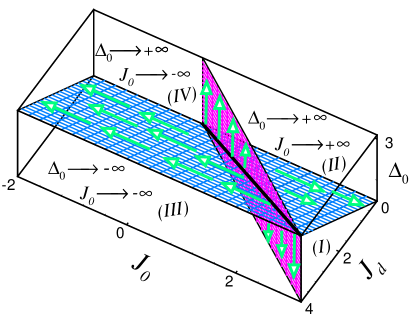
Figure 3: (Color online) Three dimensional phase diagram of four-legs spin tube in a absence of magnetic field. The blue and purple planes are critical surfaces where separate the phase diagram of model into four distinct region. The flow of couplings are different in each region. Arrows show the running of couplings under QRG. The black solid line corresponds to the critical line where the blue critical surface meets with the purple critical surface. We set $J_{1}=1.$

The QRG flow shows that the model has four stable fixed points (lines) located at ($J_{d},~{}J_{0}\rightarrow\mp\infty,~{}\Delta_{0}\rightarrow\mp\infty$) while ($J_{d},~{}J_{0}=0.8J_{d},~{}\Delta_{0}$) and ($J_{d},~{}J_{0},~{}\Delta_{0}=0.8J_{d}$) stand for the unstable fixed points which specify the critical surfaces of the model (Fig. 3). The significant result of our calculations occurs when $J_{0}\longrightarrow 0$, in which the spin nanotube decouples to four weakly interacting XXZ chains and can be analyzed by means of bosonization and conformal field theory Cabra et al. (1998, 1997). The QRG equations show that, in the presence of very small diagonal coupling, if we start with $J_{0}=0$, the ferromagnetic plaquette interaction ($J_{0}<0$) is generated under QRG transformation and runs to infinity. The generation of plaquette interaction under QRG originates from the presence of diagonal coupling.

We have linearized the QRG flow at the critical line ($J_{d},~{}J_{0}^{c}=0.8J_{d},~{}\Delta_{0}^{c}=0.8J_{d}$) (black thick solid line in Fig. 3) and found two relevant and one marginal directions. The eigenvalues of the matrix of linearized flow are $\lambda_{1}=\lambda_{2}=\frac{9}{4}$ and $\lambda_{3}=1$. The corresponding eigenvectors in the $|J_{d},J_{0},\Delta_{0}\rangle$ coordinates are $|\lambda_{1}\rangle=|0,1,0\rangle$, $|\lambda_{2}\rangle=|0,0,1\rangle$ and $|\lambda_{3}\rangle=|\frac{5}{4},1,1\rangle$. The relevant directions ($|\lambda_{1}\rangle,~{}|\lambda_{2}\rangle$) show the flow direction of plaquette coupling $J_{0}$ and plaquette anisotropy $\Delta_{0}$, respectively. The marginal direction ($|\lambda_{3}\rangle$) corresponds to the tangent line of the critical line where a critical surface ($J_{d},~{}J_{0}^{c}=0.8J_{d},~{}\Delta_{0}$) meets with a critical surface ($J_{d},~{}J_{0},~{}\Delta_{0}=0.8J_{d}$) (Fig. 3). We have also calculated the critical exponents at the critical line ($J_{d},~{}J_{0}^{c}=0.8J_{d},~{}\Delta_{0}^{c}=0.8J_{2}$) Martín-Delgado and Sierra (1996a). In this respect, we have obtained the dynamical exponent and the diverging exponent of the correlation length. The dynamical exponent is given by

$$z=\frac{\ln\Big{(}\frac{J^{\prime}_{1}}{J_{1}}\Big{)}}{\ln(n_{B})}=2,$$ (8)

where $n_{B}=3$ is the number of sites in each block. The correlation length diverges as

$$\xi\sim|J_{0}-J^{c}_{0}|^{-\nu}\sim|\Delta_{0}-\Delta^{c}_{0}|^{-\nu}$$ (9)

with exponent $\nu=1.35$, which is expressed by

$$\nu=\frac{\ln(n_{B})}{\ln\Big{(}\frac{dJ^{\prime}_{0}}{dJ_{0}}\Big{)}}=\frac{\ln(n_{B})}{\ln\Big{(}\frac{d\Delta^{\prime}_{0}}{d\Delta_{0}}\Big{)}}.$$ (10)

It is remarkable to note that, in the absence of a magnetic field, the frustrating NNN leg interaction, $J_{2}$, is generated automatically under QRG transformation by adding the second order corrections Jafari and Langari (2006, 2007). For small NNN leg interaction ($J_{2}<J_{1}$) the QRG equations show running of $J_{2}$ to zero except at the isotropic point ($\Delta_{1}=J_{1}$) where $J_{2}$ runs to the tri-critical point $J_{2}=0.155J_{1}$  Jafari and Langari (2006, 2007). To reduce complexity, in this paper the second order correction is not considered.

II.2.2 In the presence of the magnetic field: $h\neq 0$

In the presence of an external magnetic field, the QRG analysis can be done in a manner analogous to the work done in the zero magnetic field case. The only difference is that, due to the level crossing which occurs at

$$h_{1}=\frac{1}{8}\Big{(}3\Delta_{1}+\sqrt{\Delta_{1}^{2}+8J_{1}^{2}}\Big{)}=\frac{1}{4}(\Delta_{1}+\delta_{1}J_{1}),$$ (11)

for the eigenstates of the block Hamiltonian, the projection operator $P_{0}$ can be different depending on the coupling constants (see Appendix C). The first order effective Hamiltonian for $h<h_{1}$, is similar to the original one, Eq. (1), and the normalized couplings, apart from a renormalized magnetic field, is exactly the same as the zero magnetic field case, Eq. (7), and the renormalized magnetic field is given by

$$h^{\prime}=\Big{(}\frac{2+\delta_{1}^{2}}{2\delta_{1}}\Big{)}^{2}h.$$

The process of renormalization of Hamiltonian Eq. (1) for $h>h_{1}$, to the first order corrections, leads to the similar Hamiltonian with different coupling constants given in the Appendix C. In the presence of an external magnetic field, for simplicity, we restrict ourself to the case of isotropic exchange interactions in intra-leg ($\Delta_{1}=J_{1}$) and diagonal ($\Delta_{d}=J_{d}$) couplings. The running of couplings under QRG transformation for $h<h_{1}$ shows that the magnetic field increases gradually and goes beyond the level crossing point ($h_{1}$) after a few steps, which means both regions $h<h_{1}$ and $h>h_{1}$ are unique phases. Thus, it is sufficient to study the QRG-flows of the system just for $h>h_{1}$ to obtain the fixed points, critical points and the ground state phase of the system.

For $h>h_{1}$ the QRG-flows show running of leg coupling $J_{1}$ to zero, which represents the renormalization of the energy scale, and the initial isotropic case ($\Delta_{d}=J_{d}$) are not preserved under QRG transformation. Moreover, starting with any initial values of $\Delta_{1}$ and $\Delta_{d}$, the intra-leg and diagonal anisotropies run to zero, while the plaquette interaction and corresponding anisotropy go toward infinity for any initial values of $J_{0}$ and $\Delta_{0}$. It is necessary to mention that the diagonal interaction $J_{d}$ does not flow under QRG even in the presence of a magnetic field. In summary, QRG equations express that the spin tube prepared in the strong leg-coupling limit goes to the strong plaquette coupling limit which has been considered in the following section.

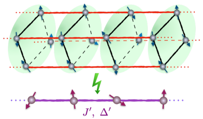
Figure 4: (Color online) A schematic decomposition of four-legs spin tube into plaquettes blocks where each plaquette replaced by an effective single site under renormalization process.

II.3 The strong plaquette coupling (Weakly interacting plaquettes): $J_{0}/J_{1,d}\rightarrow\infty$

In the strong plaquette coupling limit where we have $J_{0}/J_{1,d}\rightarrow\infty$, the plaquettes are almost decoupled, and the inter-plaquette couplings $J_{1,d}$ can be dealt with perturbatively. To apply the QRG scheme to the model in the strong plaquette coupling limit, we consider the original Hamiltonian, Eq. (1), and split the spin tube into blocks that each contains independent plaquette (see Fig. 4). In that matter, the Hilbert space of each plaquette has sixteen states including two spin-$0$ singlets, nine spin-$1$ triplets and five spin-$2$ quintuplets Gómez Albarracín et al. (2014). The four lowest eigenvalues of the plaquette Hamiltonian labeled by $e_{\alpha=0,1,2,3}$ and their corresponding eigenstates are given in the Appendix D. Because of a possible energy level crossing between these eigenstates, the projection operator, $P_{0}$, can be different depending on the coupling constants. We classify the regions corresponding two lowest eigenvalues to construct their projection operators, and we discuss the phase diagram in terms of the following five different regions:

II.3.1 Region I: $h<\Delta_{0}-J_{0}$  

In this region we consider $e_{0}$ as a ground state and $e_{2}$ as a first excited state, and to the first order corrections the effective Hamiltonian leads to the exactly solvable 1D transverse field Ising model

$${\cal H}^{eff}=-\sum_{i=1}^{N}\Big{[}J^{\prime}\sigma^{x}_{i}\sigma^{x}_{i+1}+h^{\prime}\sigma^{z}_{i}\Big{]},$$ (12)

where

$$J^{\prime}=\frac{\delta_{0}^{2}}{(2+\delta_{0}^{2})}(\Delta_{d}-\Delta_{1});\;\;\;h^{\prime}=\delta_{0}J_{0}-\Delta_{0}.$$ (13)

The 1D Ising model in a transverse field is exactly solvable by the Jordan-Wigner transformation Lieb et al. (1961) and the RSRG Martín-Delgado and Sierra (1996a). For simplicity we consider isotropic interaction on the plaquette $\Delta_{0}=J_{0}$. Then, the renormalized coupling and transverse field reduce to $J^{\prime}=(\Delta_{d}-\Delta_{1})/3$, and $h^{\prime}=J_{0}$. Phase transition between the paramagnetic and antiferromagnetic/ferromagnetic phases takes place at $h^{\prime}=J^{\prime}$ under which the system is ferromagnet ($\Delta_{1}<\Delta_{d}$) or antiferromagnet ($\Delta_{1}>\Delta_{d}$) while the system enters the paramagnetic phase above the critical point $h^{\prime}>J^{\prime}$. It is remarkable that, by assuming equal anisotropy ratios for the leg and diagonal interactions $\Delta_{1}=\Delta_{d}$ the system is always in the paramagnetic phase where spins aligned along the direction of the external magnetic field.

II.3.2 Region II: $\Delta_{0}-J_{0}<h<(\delta_{0}-1)J_{0}$  

In this region, we have $e_{0}$ as a ground state and $e_{1}$ as a first excited state. This leads the effective Hamiltonian to the well known 1D XXZ model in the presence of an external magnetic field (Appendix E), which can be solved exactly by the Bethe ansatz method Cloizeaux and Gaudin (1966); Yang and Yang (1966)

$${\cal H}^{eff}\!=\!\sum_{i=1}^{N}\Big{[}\frac{J^{\prime}}{4}(\sigma^{x}_{i}\sigma^{x}_{i+1}+\sigma^{y}_{i}\sigma^{y}_{i+1})+\frac{\Delta^{\prime}}{4}\sigma^{z}_{i}\sigma^{z}_{i+1}-\frac{h^{\prime}}{2}\sigma^{z}_{i}\Big{]}.$$ (14)

Here couplings of renormalized Hamiltonian are given by

$$\begin{aligned} J^{\prime}&=\frac{(\delta_{0}+2)^{2}}{(4+2\delta_{0}^{2})}(J_{1}-J_{d});\;\;\;\;\;\;\;\;\Delta^{\prime}=\frac{1}{4}(\Delta_{1}+\Delta_{d}),\;\;\;\;\;\;\;\;\;\;\\ h^{\prime}&=-h+(\delta_{0}-1)J_{0}+\Delta^{\prime}.\end{aligned}$$ (15)

II.3.3 Region III: $(\delta_{0}-1)J_{0}<h<\frac{1}{2}(\Delta_{0}+\delta_{0}J_{0})$  

This region is defined by the situation of $e_{1}$ as a ground state and $e_{0}$ as a first excited state, one can show that the first-order effective Hamiltonian is the same as former case, Eq. (14), with the negative field, and the couplings are defined as before, Eq. (15).

II.3.4 Region IV: $\frac{1}{2}(\Delta_{0}+\delta_{0}J_{0})<h<\Delta_{0}+J_{0}$  

For the field in this interval, $e_{1}$ is a ground state and $e_{3}$ is a first excited state, and the effective Hamiltonian is also similar to the case of regions II with different coupling constants defined by

$$J^{\prime} =(J_{1}-J_{d});\;\;\;\;\;\;~{}~{}\Delta^{\prime}=\frac{1}{4}(\Delta_{1}+\Delta_{d}),$$ (16)

$$h^{\prime} =-h+J_{0}+\Delta_{0}+3\Delta^{\prime}.$$

II.3.5 Region V: $h>\Delta_{0}+J_{0}$  

For the field which fulfills $h>\Delta_{0}+J_{0}$, $e_{3}$ is the ground state and $e_{1}$ is the first excited state. Therefore, the effective Hamiltonian up to the first order is the same as the region IV with the magnetic field in opposite direction, and the coupling constants are the same as Eq. (16).

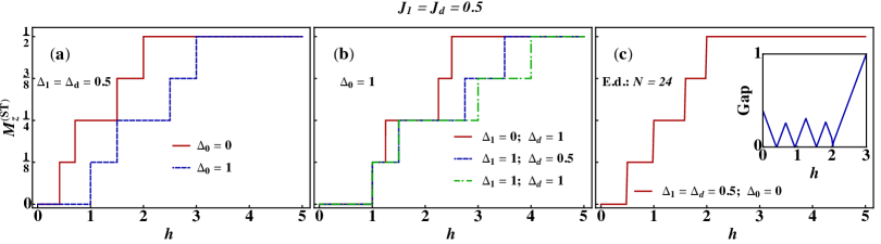
Figure 5: (Color online) Magnetization (per site) of FAFST versus the magnetic field $h$ obtained by QRG transformation on the maximum frustration line $J_{1}=J_{d}$, with couplings and anisotropic parameters: (a) $\Delta_{1}=\Delta_{d}=0.5J_{0}$ and two cases of $\Delta_{0}=0$ and $\Delta_{0}=J_{0}$, and (b) $\Delta_{0}=J_{0}$ and three cases of $\Delta_{1}=0;\;\Delta_{d}=J_{0}$, $\Delta_{1}=J_{0};\;\Delta_{d}=0.5J_{0}$, and $\Delta_{1}=J_{0};\;\Delta_{d}=J_{0}$. (c) Same quantity obtained by the numerical Lanczos results on finite spin-1/2 nanotube systems with size $N=24$, for different values of the exchanges as $\Delta_{0}=0$, and $J_{1}=\Delta_{1}=J_{d}=\Delta_{d}=0.5J_{0}$. The inset shows the corresponding energy gap. Here and in the following figures, we set $J_{0}=1$.

II.4 Phase Transition

As shown, the renormalized Hamiltonian, in the strong plaquette coupling limit, is different than the original one, FAFST, to find the recursion relation. However, the effective Hamiltonian are exactly solvable Cloizeaux and Gaudin (1966); Yang and Yang (1966); Langari (1998) and it enables us to predict distinct features of the spin tube in the strong plaquette coupling limit. To prevent the complexity, we restrict our study to the case $\Delta_{0}=J_{0}$ and $h\geq 0$. In such a case, our analysis does not cover the region I and we only consider the regions II-V, where the expected FAFST models in the presence of the magnetic field are mapped to the well-known 1D spin $1/2$ exactly solvable models.

II.4.1 First order phase transition: $J_{1}=J_{d}$

In the case of the equal inter-plaquette couplings $J_{1}=J_{d}$, the frustration is maximum, and the effective model reduces to the well-known 1D spin-1/2 Ising model in a longitudinal magnetic field,

$${\cal H}^{eff}=\frac{1}{4}\sum_{i=1}^{N}\Big{[}\Delta^{\prime}\sigma^{z}_{i}\sigma^{z}_{i+1}\pm 2h^{\prime}\sigma^{z}_{i}\Big{]},$$ (17)

The ground state properties of this model has been investigated using the RSRG method Langari (2004). This model shows a first order transition from a classical antiferromagnetic ordered phase to the saturated ferromagnetic phase at $\Delta^{\prime}=h^{\prime}$. Depends on the values of the anisotropy parameter $\Delta^{\prime}$ and the magnetic field $h^{\prime}$, the effective Hamiltonian reveals two magnetization (per site) plateaus $M_{z}^{eff}=0$ and $M_{z}^{eff}=\pm 1/2$ correspond to the antiferromagnetic and the ferromagnetic phases, respectively. Consequently, the first order phase transition points of the FAFST are given by

$$h_{c_{1}} =h_{c_{2}}=\delta_{0}-J_{0},$$ (18)

$$h_{c_{3}} =h_{c_{4}}=\delta_{0}-J_{0}+\frac{1}{2}(\Delta_{1}+\Delta_{d}),$$

$$h_{c_{5}} \!=\!h_{c_{6}}\!=J_{0}+\Delta_{0}+\frac{1}{2}(\Delta_{1}+\Delta_{d}),$$

$$h_{c_{7}} \!=\!h_{c_{8}}\!=J_{0}+\Delta_{0}+\Delta_{1}+\Delta_{d}.$$

Additionally, the magnetization in the FAFST are connected to the magnetization plateaus in the effective Hamiltonian using the renormalization equation (see the Appendix D).

For $h<\frac{1}{2}(\Delta_{0}+\delta_{0}J_{0})$ the plateaus at $M^{eff}_{z}=0$, $M^{eff}_{z}=\pm 1/2$ in the curve of magnetization (per site) versus $h^{\prime}$ in the effective model translate into plateaus at $M^{ST}_{z}=1/8$, $M^{ST}_{z}=0$, and $M^{ST}_{z}=1/4$ in the curve of magnetization (per site) versus $h$ in the FAFST. There are also renormalization equation for $h>\frac{1}{2}(\Delta_{0}+\delta_{0}J_{0})$ for linking the magnetization plateaus in the effective Hamiltonian to the magnetization curve in the FAFST (see Appendix D). In such case, plateaus at $M^{eff}_{z}=0$, $M^{eff}_{z}=\pm 1/2$ in the magnetization curve of the effective model turn into $M^{ST}_{z}=1/4$, $M^{ST}_{z}=3/8$ and $M^{ST}_{z}=1/2$ in the magnetization curve of the FAFST model.

The magnetization curves of FAFST along the maximum frustration line $(J_{1}=J_{d})$ have been shown in Figs. 5(a and b) based on the numerical RSRG results. To examine the anisotropy effects, the magnetization curves of FAFST have been plotted versus the magnetic field $h$ for different values of anisotropies. Notice that in Fig. 5(a) the magnetization plateaus has been depicted versus $h$ for isotropic case $\Delta_{0}=J_{0},J_{1}=\Delta_{1},J_{d}=\Delta_{d}$ (dashed-blue curve) which shows quantitatively excellent agreement with numerical density matrix renormalization group results Gómez Albarracín et al. (2014). This result indicates that the RSRG is a good approach to study the critical behavior of FAFST in the thermodynamic limit.

To examine the anisotropy effects, the magnetization curves of FAFST have been plotted versus the magnetic field $h$ in Fig. 5 for different values of anisotropies. As seen, the location of critical points and the width of the magnetization plateaus are controlled by the anisotropies according to Eq. (18). It is to be noted that, the renormalized subspace specified by the singlet $(e_{0})$ and triplet $(e_{1})$ states is separate at the level crossing point $h_{l}=\frac{1}{2}(\Delta_{0}+\delta_{0}J_{0})$ from the renormalized subspace defined by the triplet $(e_{1})$ and quintuplet $(e_{3})$ states. Therefore, for the cases that $h_{c_{3}}~{}(=h_{c_{4}})$ is greater than $h_{l}$, the point $h_{c_{3}}$ is not the critical point and the level crossing point would be a first order phase transition point (Figs. 5(a)-(b)). From Fig. 5(b) one can clearly see that the width of $M^{(ST)}_{z}=1/8$ and $M^{(ST)}_{z}=3/8$ plateaus reduced by decreasing the inter-plaquette anisotropies ($\Delta_{1}+\Delta_{d}$).

To accomplishment of our study, using the numerical Lanczos method we have studied the effect of the external magnetic field on the ground state magnetic phase diagram of the mentioned FAFST model. In Fig. 5(c), we have presented our numerical results. In this figure on top of the magnetization, in the inset we plot the energy gap as a function of the magnetic field for a tube size $N=24$ and different values of the exchanges according to the $\Delta_{0}=0$, $J_{1}=\Delta_{1}=0.5J_{0}$ and $J_{d}=\Delta_{d}=0.5J_{0}$. As is seen, in the absence of the magnetic field the FAFST model is gapped. By increasing the magnetic field, the energy gap decreases linearly and vanishes at the first critical field. By more increasing the magnetic field, the energy gap will be closed in other three critical magnetic fields, independent of the system size. After the fourth critical field, the gap opens again and for a sufficiently large field becomes proportional to the magnetic field which is known as the indication of the ferromagnetic phase. On the other hand, the magnetization is zero in the absence of the magnetic field at zero temperature. By increasing the magnetic field, besides the zero and saturation plateaus, three magnetization plateau at $M=1/8,M=2/8,M=3/8$ are observed. We have to mention that the critical fields estimated by the numerical Lanczos method are in complete agreement with our analytical results presented in figures Fig. 5(a).

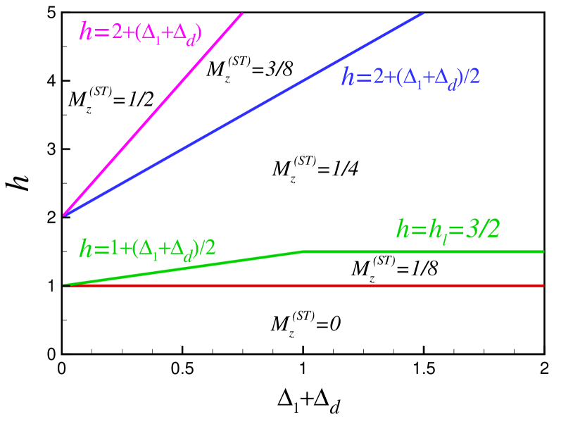
Figure 6: (Color online) The phase diagram: $h$ vs $(\Delta_{1}+\Delta_{d})$ along the line $J_{1}=J_{2}$ obtained by QRG transformation for $\Delta_{0}=J_{0}=1$.

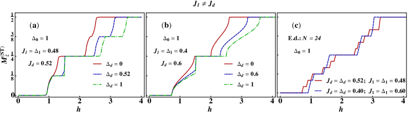
Figure 7: (Color online) Magnetization (per site) of FAFST versus the magnetic field $h$ obtained by QRG transformation for $J_{1}\neq J_{d}$ cases, with couplings and anisotropic parameters: (a) $\Delta_{0}=J_{0};\;J_{1}=\Delta_{1}=0.48J_{0};\;J_{d}=0.52J_{0}$ and three cases of $\Delta_{d}=(0,0.52,1)J_{0}$, and (b) $\Delta_{0}=J_{0};\;J_{1}=\Delta_{1}=0.4J_{0};\;J_{d}=0.6J_{0}$ and three cases of $\Delta_{d}=(0,0.6,1)J_{0}$. (c) Numerical Lanczos results of the same quantity on finite spin-1/2 nanotube systems with the system size $N=24$. We set $\Delta_{0}=J_{0}$, and the rest of exchanges are considered for two set of parameters as $J_{1}=\Delta_{1}=0.48J_{0};\;J_{d}=\Delta_{d}=0.52J_{0}$ (solid-red) and $J_{1}=\Delta_{1}=0.4J_{0};\;J_{d}=\Delta_{d}=0.6J_{0}$ (dashed-blue).

The magnetic phases of FAFST along maximum frustration line $J_{1}=J_{d}$ has been shown versus $(\Delta_{1}+\Delta_{d})$ and $h$ in Fig. 6 for $\Delta_{0}=J_{0}$, based on the RSRG approach. As it can be observed, $M^{(ST)}_{z}=3/8$ and $M^{(ST)}_{z}=1/2$, plateaus width linearly increase with frustrating anisotropy $(\Delta_{1}+\Delta_{d})$, while width of $M^{(ST)}_{z}=1/8$ plateau initially increases linearly with $(\Delta_{1}+\Delta_{d})$ and then at $h_{l}$ point reaches to the constant value.

It would be worth mentioning that although at the isotropic point: $\Delta_{0}=J_{0},J_{1}=\Delta_{1},J_{d}=\Delta_{d}$, the critical points of FAFST, Eq. (18), reduces to the critical points expression obtained by low energy effective method Gómez Albarracín et al. (2014), but the magnetic phase obtained by QRG method is not the same as that of obtained by the low energy effective method Gómez Albarracín et al. (2014). This discrepancy originates from the presence of level crossing point $h_{l}$, where the system shows first order first transition. The low energy effective method is incapable of capturing the effect of this level crossing point even away from the maximum frustration line $J_{1}=J_{d}$.

II.4.2 Second order phase transition: $J_{1}\neq J_{d}$

As we mentioned previously, in the case where inter-plaquette couplings are not equal $J_{1}\neq J_{d}$, the FAFST Hamiltonian maps to the effective Hamiltonian, the 1D spin 1/2 XXZ chain in the presence of the longitudinal magnetic field. This model is exactly solvable by means the Bethe ansatz method. Moreover, the properties of the XXZ model in the presence of a magnetic field has been studied using the QRG method Langari (1998). In this subsection we study the effective Hamiltonian, by combining a Jordan-Wigner transformation Lieb et al. (1961) with a mean-field approximation Caux et al. (2003) (see Appendix E). Then by using the renormalization equations which connects the magnetization of the effective model to that of FAFST, we can obtain the magnetization of the FAFST. Therefore, it is useful to briefly review the main features of the 1D XXZ chain in the presence of the magnetic field.

In absence of a magnetic field $h^{\prime}=0$, for $\Delta^{\prime}=J_{0}$, the Hamitonian is $SU(2)$ symmetry invariant, but for $\Delta^{\prime}\neq J_{0}$ the $SU(2)$ symmetry breaks down to the $U(1)$ rotational symmetry around the $z$-axis. It is known that for planar anisotropy $-J_{0}\leq\Delta^{\prime}\leq J_{0}$ the model is not supporting any kind of long range order where the correlations decay algebraic and the ground state is gapless Haldane (1980), so called Luttinger liquid phase. Enhancing the amount of anisotropy stabilizes the spin alignment. For $\Delta^{\prime}>J_{0}$, the symmetry of the ground state is reduced to $Z_{2}$ and the ground state is the gapped Nèel ordered state which is in the universality class of 1D antiferromagnetic Ising chain. Indeed, the third term in the Hamiltonian Eq. (14) causes Nèel ordering in the system while the first two terms in the Hamiltonian extend the quantum fluctuations in the system and result in the corruption of the ordering. Furthermore, for $\Delta<-J_{0}$ the ground state is the gapfull ferromagnetic state.

In presence of a magnetic field $h^{\prime}\neq 0$, there are two critical lines $h_{c1}$ and $h_{c2}$ restricting Luttinger liquid phase between ferromagnetic and Nèel phases which are given by following equations Yang and Yang (1966)

$$\begin{aligned} &h_{c1}=J^{\prime}\sinh g\sum_{n=-\infty}^{+\infty}\frac{(-1)^{n}}{\cosh(ng)};\\ &h_{c2}=\pm\Big{(}1+\frac{\Delta^{\prime}}{J_{0}}\Big{)}|J^{\prime}|,\end{aligned}$$ (19)

with $g=\cosh^{-1}(\frac{\Delta^{\prime}}{J_{0}}).$ For $\Delta^{\prime}>J_{0}$ and small magnetic fields $h^{\prime}<h_{c}$ the ground state is still the Nèel ordered state. This state exhibits a gap in the excitation spectrum whose value at $h^{\prime}=0$ corresponds to $h_{c1}$. In particular, it is exponentially small close to the Heisenberg point at $\Delta^{\prime}=J_{0}$, which is characteristic for a Kosterlitz-Thouless transition Kosterlitz and Thouless (1973); Kosterlitz (1974). The Luttinger-liquid state exists for $|\Delta^{\prime}|<J_{0}$, $h^{\prime}<h_{c2}$ and $\Delta^{\prime}>J_{0}$, $h_{c1}<h^{\prime}<h_{c2}$. Finally, phase transition between Luttinger-liquid and ferromagnetic occurs at $h=h_{c_{2}}$ under which the ground state is the ferromagnetically polarized state along the $z$-direction.

To study the effect of anisotropy, the magnetization of FAFST is plotted versus the magnetic field in Fig. 7, for different values of anisotropies. It can be clearly seen that, $M^{(ST)}_{z}=1/8$ and $M^{(ST)}_{z}=3/8$ plateaus width enhances (reduces) by increasing (decreasing) the inter-plaquette anisotropies ($\Delta_{1},\Delta_{d}$), and the first order phase transition point at $h_{l}$ fades out gradually by decreasing $\Delta_{1}$ and $\Delta_{d}$. As seen, for a small deviations from the maximum frustrated line $J_{1}=0.48J_{0},J_{d}=0.52J_{0}$, width of $M^{(ST)}_{z}=1/8$ and $M^{(ST)}_{z}=3/8$ plateaus reduce, and jumps between plateaus change to smooth curves which is feature of Luttinger liquid phases. As represented in Fig. 7(b), $M^{(ST)}_{z}=1/8$ and $M^{(ST)}_{z}=3/8$ magnetization plateaus are not present for $J_{1}=0.4J_{0},J_{d}=0.6J_{0}$. Away from the maximum frustrated line, the magnetization shows only a gapless Luttinger liquid phase, which means the system consists of decoupled spin-1/2 chains. In other words, the presence of $M^{(ST)}_{z}=1/8$ and $M^{(ST)}_{z}=3/8$ plateaus is very sensitive to frustration.

Again we have implemented our numerical Lanczos algorithm on the mentioned FAFST model. In Fig. 7(c), we have presented our numerical results for different values of the anisotropy parameters. In this figure, the magnetization for a size $N=24$ is plotted as a function of the magnetic field for two set of anisotropy parameters according to $\Delta_{0}=J_{0}$; $J_{1}=\Delta_{1}=0.48J_{0}$, $J_{d}=\Delta_{d}=0.52J_{0}$ and $\Delta_{0}=J_{0}$; $J_{1}=\Delta_{1}=0.4J_{0}$, $J_{d}=\Delta_{d}=0.6J_{0}$. As is seen in this figure, the place and width of magnetic plateaues are in complete agreement with the analytical results presented in Fig. 7(b). One should note that observed oscillations of the magnetization in the Fig. 7(c) are arised from the level crossings in the finite size systems.

Inspecting the effect of anisotropy, clearly shows the $M^{(ST)}_{z}=1/8$ and $M^{(ST)}_{z}=3/8$ plateaus width enhances (reduces) by increasing (decreasing) the inter-plaquette anisotropies ($\Delta_{1},\Delta_{d}$), and the first order phase transition point at $h_{l}$ fades out gradually by decreasing $\Delta_{1}$ and $\Delta_{d}$. To summarize, for small deviation from maximum frustrating line, the one-eight and third-eight magnetization plateaus width, which are sensitive to frustration, can be controlled by the intra-plaquette anisotropies. Away from the maximum frustrating line, where the one-eighth and three-eighth magnetization plateaus are absent, the intra-plaquette anisotropies can affect the width of one-quarter magnetization plateau.

III Summary

We survey a geometrically frustrated anisotropic four-leg spin tube in the absence/presence of the magnetic field using the quantum real Space Renormalization group. We show that in the limit of the strong leg coupling the diagonal frustrating interaction does not fellow under renormalization transformation. Moreover, in the limit of the strong leg coupling, the spin tube goes to the strong plaquette coupling limit, i.e., weakly interacting plaquettes. Our study indicates that in the weakly interacting plaquettes, FAFST maps onto the 1D spin-1/2 XXZ model under renormalization transformation. For the case that the leg and frustrating couplings are the same (maximum frustrating line), the FAFST Hamiltonian reveals only first order quantum phase transitions at zero temperature. In such a case, fractional magnetization plateaus at zero, one-quarter, one-half and three-quarter of the saturation magnetization are exhibited. Also, the magnetization plateaus at one-quarter and three-quarter of the saturation magnetization show the highest sensitivity to frustration and washed out away from the maximum frustrating line. Comparing the QRG to the density matrix renormalization group results guaranteed that the real space renormalization group method is a remarkable approach to study the critical behavior of FAFST in the thermodynamic limit. We have also calculated the classical phase diagram by considering the spin structure as a spiral Arlego and Brenig (2011). The result show that $M^{ST}_{z}=0$ and $M^{ST}_{z}=1/2$ can be captured by classical spin while, absence of $M^{ST}_{z}=1/8$, $M^{ST}_{z}=1/4$, and $M^{ST}_{z}=3/8$, shows that they are originated from quantum effect (frustration).

At the end, attention should be paid to the importance of the exploration of quantum correlation, such as entanglement and quantum discord in the FAFST model. They can be easily done in the thermodynamics limit by applying the real Space Renormalization group method Usman et al. (2015); Jafari (2013); Langari and Rezakhani (2012); Jafari (2010); Jafari et al. (2008). In particular, studying the four-leg spin tube frustrated by next-nearest-neighbor interaction on the leg, is an interesting topic that clearly deserves future investigations, which are not considered in the current work.

Appendices

Appendix A Real Space Renormalization Group (RSRG)

When dealing with zero temperature properties of many-body systems with a large number of strongly correlated degrees of freedom, one can consider real space renormalization Group (RSRG) as a one of the possible and powerful methods Martín-Delgado and Sierra (1996b, a); Langari (2004); Langari and Rezakhani (2012). Where, its application on lattice systems implies the construction of a new smaller system corresponding to the original one with new (renormalized) interactions between the degrees of freedom Farajollahpour and Jafari (2018); Jafari (2017); Jafari et al. (2017). One of the tasks of QRG is to obtain the recursion relation, which define the transformation of old couplings into new ones. In the Kadanoffs representation, analyzing such recursion relation determines qualitatively the structure of the phase diagram; approximately locates the critical/fixed points and obtains the critical exponents Martín-Delgado and Sierra (1996a); Langari (2004); Jafari and Langari (2007). This method divides a lattice into disconnected blocks of $n_{B}$ sites each where the Hamiltonian is exactly diagonalized. This partition of the lattice into blocks induces a decomposition of the Hamiltonian ${\cal H}$ into an intrablock Hamiltonian ${\cal H}_{B}$ and a interblock Hamiltonian ${\cal H}^{BB}$, where the block Hamiltonian ${\cal H}^{B}$ is a sum of commuting terms, ${\cal H}^{B}=\sum_{I=1}^{n/n_{B}}h^{B}_{I}$, each acting on different ($I$th) blocks of chain. Each block is treated independently to build the projection operator $P_{0}$ onto the lower energy subspace. The projection of the Hamiltonian is mapped to an effective Hamiltonian ${\cal H}^{eff}$ acts on the renormalized subspace. Thus, in perturbative approach, the effective Hamiltonian up to first order corrections is given by Martín-Delgado and Sierra (1996a)

$${\cal H}^{eff}={\cal H}_{0}^{eff}+{\cal H}_{1}^{eff},$$ (20)

with

$${\cal H}_{0}^{eff}=P_{0}{\cal H}^{B}P_{0};\;\;\;\;{\cal H}_{1}^{eff}=P_{0}{\cal H}^{BB}P_{0}.$$

Appendix B The intrea-block and intre-block Hamiltonians of three sites, its eigenvectors and eigenvalues in the absence of magnetic field

The inter-block ${\cal H}^{BB}$ and intra-block ${\cal H}^{B}$ Hamiltonians for the three sites decomposition are

$$h_{I}^{B}=\frac{1}{4} \sum_{\alpha=1}^{4}\Bigg{[}J_{1}\Big{(}\sigma^{x}_{1,\alpha,I}\sigma^{x}_{2,\alpha,I}+\sigma^{y}_{1,\alpha,I}\sigma^{y}_{2,\alpha,I}+\sigma^{x}_{2,\alpha,I}\sigma^{x}_{3,\alpha,I}$$ (21)

$$+\sigma^{y}_{2,n,I}\sigma^{y}_{3,\alpha,I}\Big{)}+\Delta_{1}\Big{(}\sigma^{z}_{1,\alpha,I}\sigma^{z}_{2,\alpha,I}+\sigma^{z}_{2,\alpha,I}\sigma^{z}_{3,\alpha,I}\Big{)}\Bigg{]};$$

$$H^{BB}=\frac{1}{4}\sum_{I=1}^{N/3}\sum_{\alpha=1}^{4}\Bigg{[}$$ (22)

$$J_{1}\Big{(}\sigma_{3,\alpha,I}^{x}\sigma_{1,\alpha,I+1}^{x}+\sigma_{3,\alpha,I}^{y}\sigma_{1,\alpha,I+1}^{y}\Big{)}+\Delta_{1}\sigma_{3,\alpha,I}^{z}\sigma_{1,\alpha,I+1}^{z}$$

$$+J_{0}\Big{(}\sigma_{1,\alpha,I}^{x}\sigma_{1,\alpha+1,I}^{x}+\sigma_{2,\alpha,I}^{x}\sigma_{2,\alpha+1,I}^{x}+\sigma_{3,\alpha,I}^{x}\sigma_{3,\alpha+1,I}^{x}$$

$$+\sigma_{1,\alpha,I}^{y}\sigma_{1,\alpha+1,I}^{y}+\sigma_{2,\alpha,I}^{y}\sigma_{2,\alpha+1,I}^{y}+\sigma_{3,\alpha,I}^{y}\sigma_{3,\alpha+1,I}^{y}\Big{)}$$

$$+\Delta_{0}\Big{(}\sigma_{1,\alpha,I}^{z}\sigma_{1,\alpha+1,I}^{z}+\sigma_{2,\alpha,I}^{z}\sigma_{2,\alpha+1,I}^{z}+\sigma_{3,\alpha,I}^{z}\sigma_{3,\alpha+1,I}^{z}\Big{)}$$

$$+J_{d}\Big{(}\sigma_{3,\alpha,I}^{x}\sigma_{1,\alpha+1,I+1}^{x}+\sigma_{3,\alpha,I}^{y}\sigma_{1,\alpha+,I+1}^{y}\Big{)}$$

$$+\Delta_{d}\sigma_{3,\alpha,I}^{z}\sigma_{1,\alpha+1,I+1}^{z}\Bigg{]},$$

where $\sigma_{j,\alpha,I}^{\mu}$ refers to the $\mu$-component of the Pauli matrix at site $j$ of the block labeled by $I$ with itra-plaquettes label $\alpha$. The exact treatment of this Hamiltonian leads to four distinct eigenvalues which are doubly degenerate. The ground, first, second and third excited state energies have the following expressions in terms of the coupling constants:

$$e_{0}=-\frac{1}{2}\delta_{1}J_{1};\;\;e_{1}=\frac{1}{2}\delta^{\prime}_{1}J_{1};\;\;e_{2}=0;\;\;e_{3}=\frac{\Delta_{1}}{2},$$ (23)

with corresponding eigenfunctions

$$|\psi_{0}\rangle=\frac{1}{\sqrt{2+\delta_{1}^{2}}}(|\uparrow\uparrow\downarrow\rangle-\delta_{1}|\uparrow\downarrow\uparrow\rangle+|\downarrow\uparrow\uparrow\rangle),$$ (24)

$$|\psi_{0}^{\prime}\rangle=\frac{1}{\sqrt{2+\delta_{1}^{2}}}(|\uparrow\downarrow\downarrow\rangle-\delta_{1}|\downarrow\uparrow\downarrow\rangle+|\downarrow\downarrow\uparrow\rangle),$$

$$|\psi_{1}\rangle=\frac{1}{\sqrt{2+\delta_{1}^{{}^{\prime}2}}}(|\uparrow\uparrow\downarrow\rangle+\delta^{\prime}_{1}|\uparrow\downarrow\uparrow\rangle+|\downarrow\uparrow\uparrow\rangle),$$

$$|\psi_{1}^{\prime}\rangle=\frac{1}{\sqrt{2+\delta_{1}^{{}^{\prime}2}}}(|\uparrow\downarrow\downarrow\rangle+\delta^{\prime}_{1}|\downarrow\uparrow\downarrow\rangle+|\downarrow\downarrow\uparrow\rangle),$$

$$|\psi_{2}\rangle=\frac{1}{\sqrt{2}}(|\downarrow\downarrow\uparrow\rangle-|\uparrow\downarrow\downarrow\rangle),$$

$$|\psi_{2}^{\prime}\rangle=\frac{1}{\sqrt{2}}(|\uparrow\uparrow\downarrow\rangle-|\downarrow\uparrow\uparrow\rangle),$$

$$|\psi_{3}\rangle=|\uparrow\uparrow\uparrow\rangle,$$

$$|\psi_{3}^{\prime}\rangle=|\downarrow\downarrow\downarrow\rangle,$$

where

$$\delta^{\prime}_{n}=\delta_{n}-\frac{\Delta_{n}}{J_{n}}=\frac{1}{2J_{n}}\Big{[}\sqrt{\Delta_{n}^{2}+8J_{n}^{2}}-\Delta_{n}\Big{]},$$ (25)

and we consider $|\uparrow\rangle$ and $|\downarrow\rangle$ as the eigenstates of $\sigma^{z}$.

Appendix C The intrea-block and intre-block Hamiltonians of three sites, its eigenvectors and eigenvalues in the presence of magnetic field

In the present of field the inter-block Hamiltonian for the three sites decomposition are

$$h_{I}^{B}= \sum_{\alpha=1}^{4}\frac{1}{4}\Bigg{[}J_{1}\Big{(}\sigma^{x}_{1,\alpha,I}\sigma^{x}_{2,\alpha,I}+\sigma^{y}_{1,\alpha,I}\sigma^{y}_{2,\alpha,I}+\sigma^{x}_{2,\alpha,I}\sigma^{x}_{3,\alpha,I}$$ (26)

$$+\sigma^{y}_{2,\alpha,I}\sigma^{y}_{3,\alpha,I}\Big{)}+\Delta_{1}\Big{(}\sigma^{z}_{1,\alpha,I}\sigma^{z}_{2,\alpha,I}+\sigma^{z}_{2,\alpha,I}\sigma^{z}_{3,\alpha,I}\Big{)}$$

$$-2h(\sigma^{z}_{1,\alpha,I}+\sigma^{z}_{2,\alpha,I}+\sigma^{z}_{3,\alpha,I})\Bigg{]},$$

and intra-block Hamiltonian ${\cal H}^{BB}$ is defined in similar way as Eq. (22). The ground, first, second and third excited state energies have the following expressions in terms of the coupling constants:

$$\begin{aligned} &e_{0/1}=-\frac{1}{2}(\pm h+\delta_{1});\;\;\;e_{2}=\frac{1}{4}(2\Delta_{1}-6h);\;\;\;e_{3}=-\frac{1}{2}h;\;\;\;\\ &e_{4/5}=\frac{1}{2}\Big{[}\mp h+\delta^{\prime}_{1}\Big{]};\;\;\;\;e_{6}=\frac{1}{2}h;\;\;\;\;e_{7}=\frac{1}{2}(\Delta_{1}+6h),\end{aligned}$$

with following eigenfunctions

$$\begin{aligned} &|\psi_{0}\rangle=\frac{1}{\sqrt{2+\delta_{1}^{2}}}(|\uparrow\uparrow\downarrow\rangle-\delta_{1}|\uparrow\downarrow\uparrow\rangle+|\downarrow\uparrow\uparrow\rangle),\\ &|\psi_{1}\rangle=\frac{1}{\sqrt{2+\delta_{1}^{2}}}(|\uparrow\downarrow\downarrow\rangle-\delta_{1}|\downarrow\uparrow\downarrow\rangle+|\downarrow\downarrow\uparrow\rangle),\\ &|\psi_{2}\rangle=|\uparrow\uparrow\uparrow\rangle,\\ &|\psi_{3}\rangle=\frac{1}{\sqrt{2}}(|\downarrow\uparrow\uparrow\rangle-|\uparrow\uparrow\downarrow\rangle),\\ &|\psi_{4}\rangle=\frac{1}{\sqrt{2+\delta_{1}^{{}^{\prime}2}}}(|\uparrow\uparrow\downarrow\rangle+\delta^{\prime}_{1}|\uparrow\downarrow\uparrow\rangle+|\downarrow\uparrow\uparrow\rangle),\\ &|\psi_{5}\rangle=\frac{1}{\sqrt{2+\delta_{1}^{{}^{\prime}2}}}(|\uparrow\downarrow\downarrow\rangle+\delta^{\prime}_{1}|\downarrow\uparrow\downarrow\rangle+|\downarrow\downarrow\uparrow\rangle),\;\;\;\;\\ &|\psi_{6}\rangle=\frac{1}{\sqrt{2}}(|\downarrow\downarrow\uparrow\rangle-|\uparrow\downarrow\downarrow\rangle),\\ &|\psi_{7}\rangle=|\downarrow\downarrow\downarrow\rangle.\end{aligned}$$ (27)

The renormalized and rescaled coupling constants for $h>h_{1}$ are defined by

$$\begin{aligned} J^{\prime}_{1}=&J_{1};\;\;\;\;\;\;\;\;\;\;\Delta^{\prime}_{1}=(\frac{1}{2+\delta_{1}^{2}})\Delta_{1},\\ J^{\prime}_{d}=&J_{d};\;\;\;\;\;\ \;\;\;\;\Delta^{\prime}_{d}=(\frac{1}{2+\delta_{1}^{2}})\Delta_{d},\\ J^{\prime}_{0}=&-2\delta_{1}J_{d}+(2+\delta_{1}^{2})J_{0},\\ \Delta^{\prime}_{0}=&(\frac{2\delta_{1}^{2}}{2+\delta_{1}^{2}})\Delta_{d}+(\frac{2+\delta_{1}^{4}}{2+\delta_{1}^{2}})\Delta_{0},\\ h^{\prime}=&(2+\delta_{1}^{2})(-h+\Delta_{1}+\delta_{1}J_{1})+2(\frac{1+\delta_{1}^{2}}{2+\delta_{1}^{2}})\Delta_{1}\;\;\;\;\\ &+2(\frac{5+3\delta_{1}^{2}+2\delta_{1}^{4}}{2+\delta_{1}^{2}})\Delta_{d}+2(\frac{2+4\delta_{1}^{2}}{2+\delta_{1}^{2}})\Delta_{0}.\end{aligned}$$ (28)

Here the rescaling factor is $\varepsilon^{\prime}_{1}=(\frac{1}{2+\delta_{1}^{2}})$.

Appendix D The plaquette Hamiltonian, four lowest eigenvalues of plaquette Hamiltonian and their corresponding eigenstates in weak leg couplings

In the strong plaquette coupling (Weakly interacting plaquettes: $J_{0}/J_{1,d}\rightarrow\infty$) one can write the inter-block and intra-block Hamiltonians for the plaquette decomposition as

$$h_{I}^{B}=\frac{1}{4} \Bigg{[}J_{0}\Big{(}\sigma^{x}_{1,I}\sigma^{x}_{2,I}+\sigma^{x}_{2,I}\sigma^{x}_{3,I}+\sigma^{x}_{3,I}\sigma^{x}_{4,I}+\sigma^{x}_{4,I}\sigma^{x}_{1,I}$$

$$+\sigma^{y}_{1,I}\sigma^{y}_{2,I}+\sigma^{y}_{2,I}\sigma^{y}_{3,I}+\sigma^{y}_{3,I}\sigma^{y}_{4,I}+\sigma^{y}_{4,I}\sigma^{y}_{1,I}\Big{)}$$

$$+\Delta_{0}\Big{(}\sigma^{z}_{1,I}\sigma^{z}_{2,I}+\sigma^{z}_{2,I}\sigma^{z}_{3,I}+\sigma^{z}_{3,I}\sigma^{z}_{4,I}+\sigma^{z}_{4,I}\sigma^{z}_{1,I}\Big{)}$$

$$-2h\Big{(}\sigma^{z}_{1,I}+\sigma^{z}_{2,I}+\sigma^{z}_{3,I}+\sigma^{z}_{4,I}\Big{)}\Bigg{]},$$

and

$${\cal H}^{BB} \!=\frac{1}{4}\sum_{I=1}^{N}\Bigg{[}\Delta_{d}\Big{(}\sigma_{1,I}^{z}\sigma_{2,I+1}^{z}+\sigma_{2,I}^{z}\sigma_{3,I+1}^{z}+\sigma_{3,I}^{z}\sigma_{4,I+1}^{z}\Big{)}$$

$$+\!\sum_{\alpha=1}^{4}\Big{[}\!J_{1}\Big{(}\sigma_{\alpha,I}^{x}\sigma_{\alpha,I+1}^{x}+\sigma_{\alpha,I}^{y}\sigma_{\alpha,I+1}^{y}\Big{)}\!+\!\Delta_{1}\sigma_{\alpha,I}^{z}\sigma_{\alpha,I+1}^{z}\Big{]}$$

$$+J_{d}\Big{(}\sigma_{1,I}^{x}\sigma_{2,I+1}^{x}+\sigma_{2,I}^{x}\sigma_{3,I+1}^{x}+\sigma_{3,I}^{x}\sigma_{4,I+1}^{x}$$

$$\hskip 28.45274pt+\sigma_{1,I}^{y}\sigma_{2,I+1}^{y}+\sigma_{2,I}^{y}\sigma_{3,I+1}^{y}+\sigma_{3,I}^{y}\sigma_{4,I+1}^{y}\Big{)}\Bigg{]},$$

here $\sigma_{\alpha,I}^{\mu}$ refers to the $\mu$-component of the Pauli matrix at the block labeled by $I$ with itra-plaquettes label $\alpha$. The eigenstates are obtained by

$$|\psi_{0}\rangle= \frac{1}{\sqrt{4+2\delta_{0}^{2}}}(|\uparrow\uparrow\downarrow\downarrow\rangle-\delta_{0}|\uparrow\downarrow\uparrow\downarrow\rangle+|\downarrow\uparrow\uparrow\downarrow\rangle$$ (29)

$$-\delta_{0}|\downarrow\uparrow\downarrow\uparrow\rangle+|\downarrow\downarrow\uparrow\uparrow\rangle+|\uparrow\downarrow\downarrow\uparrow\rangle),\;\;\;$$

$$|\psi_{1}\rangle= \frac{1}{2}(|\uparrow\uparrow\downarrow\uparrow\rangle-|\uparrow\uparrow\uparrow\downarrow\rangle+|\downarrow\uparrow\uparrow\uparrow\rangle-|\uparrow\downarrow\uparrow\uparrow\rangle),$$

$$|\psi_{2}\rangle= \frac{1}{\sqrt{2}}(|\downarrow\uparrow\downarrow\uparrow\rangle-|\uparrow\downarrow\uparrow\downarrow\rangle)$$

$$|\psi_{3}\rangle= |\uparrow\uparrow\uparrow\uparrow\rangle,$$

and corresponding eigenvalues are given by

$$e_{0}=-\delta_{0}J_{0};\;\;e_{1}=-(J_{0}+h);\;\;e_{2}=-\Delta_{0};\;\;e_{3}=(\Delta_{0}-2h).$$

The magnetization (per site) in the effective Hamiltonian $M^{eff}_{z}$ linked to the magnetization (per site) of the spin tube $M^{ST}_{z}$ through the renormalization transformation of the $\sigma^{z}$ component of the Pauli matrices. The $\sigma^{z}$ in the effective Hilbert space has the following transformations ($\alpha=1,2,3,4$) for each region:

• II: $P_{0}^{I}\sigma_{\alpha,I}^{z}P_{0}^{I}=\frac{1}{4}(1-\sigma_{I}^{z});~{}~{}M^{ST}_{z}=\frac{1}{8}(1-2M^{eff}_{z})$,

• III: $P_{0}^{I}\sigma_{\alpha,I}^{z}P_{0}^{I}=\frac{1}{4}(1+\sigma_{I}^{z});~{}M^{ST}_{z}=\frac{1}{8}(1+2M^{eff}_{z})$,

• IV: $P_{0}^{I}\sigma_{\alpha,I}^{z}P_{0}^{I}=\frac{1}{4}(3-\sigma_{I}^{z});~{}M^{ST}_{z}=\frac{1}{8}(3-2M^{eff}_{z})$,

• V: $P_{0}^{I}\sigma_{\alpha,I}^{z}P_{0}^{I}=\frac{1}{4}(3+\sigma_{I}^{z});~{}~{}M^{ST}_{z}=\frac{1}{8}(3+2M^{eff}_{z})$.

Appendix E Mean field approximation

One of the analytical approaches to study the renormalized 1D spin-1/2 XXZ Hamiltonian (Eq. (14)) is the fermionization technique. In this respect, by applying the Jordan-Wigner transformation Lieb et al. (1961) the effective XXZ Hamiltonian maps onto a system of interacting spinless fermionsDmitriev et al. (2002):

$${\cal H}=\sum_{i} \Big{[}\frac{J^{\prime}}{2}(c^{{\dagger}}_{i}c_{i+1}+c^{{\dagger}}_{i+1}c_{i})+\Delta^{\prime}c^{{\dagger}}_{i}c_{i}c^{{\dagger}}_{i+1}c_{i+1}\Big{]}$$ (30)

$$-(h^{\prime}+\Delta^{\prime})\sum_{i}c^{{\dagger}}_{i}c_{i}.$$

It is known that the fermion interaction term can be decomposed by following relevant order parameters which are related to spin-spin correlation functions asDmitriev et al. (2002)

$$\gamma_{1} =\langle c^{{\dagger}}_{i}c_{i}\rangle;\;\;\;~{}\gamma_{2} =\langle c^{{\dagger}}_{i}c_{i+1}\rangle,$$ (31)

Using $c^{{\dagger}}_{i}=\frac{1}{\sqrt{N}}\sum^{N}_{n=1}e^{ikn}c^{{\dagger}}_{k}$, the Fourier transformation to momentum space is performed and then the diagonalized Hamiltonian is obtained as

$${\cal H}=\sum_{k}\varepsilon(k)c^{{\dagger}}_{k}c_{k},$$ (32)

where the energy spectrum is

$$\varepsilon(k)=(J-2\gamma_{2}\Delta)\cos(k)-(h+\Delta-2\gamma_{1}\Delta).$$ (33)

Easily, one can show that the Fermi points are given by

$$\pm k_{F}=\pm\arccos\!\Bigg{[}\frac{h+\Delta-2\gamma_{1}\Delta}{J-2\gamma_{2}\Delta}\Bigg{]}.$$ (34)

One should note that the following equations should be satisfied self-consistently

$$\gamma_{1}=1-\frac{k_{F}}{\pi},~{}\gamma_{2}=-\frac{\sin(k_{F})}{\pi},$$ (35)

Finally, the magnetization is obtained as

$$\begin{aligned} M=\left\{\begin{array}[]{ll}\frac{1}{2}&\hskip 35.56593pth>h_{c}\\ -\frac{1}{2}&\hskip 35.56593pth<-h_{c}\\ \frac{1}{2}-\frac{k_{F}}{\pi}&\hskip 21.33955pt-h_{c}<h<h_{c}\end{array}\right.\end{aligned}$$ (36)

References

- Claudine et al. (2011) L. Claudine, M. Philippe, and M. Frédéric, eds., “Introduction to frustrated magnetism,” (Springer-Verlag Berlin Heidelberg, 2011) p. 682.
- Hung (2013) D. Hung, The, ed., “Frustrated spin systems,” (World Scientific Publishing Company, 2013) p. 682.
- Jafari and Langari (2007) R. Jafari and A. Langari, Phys. Rev. B 76, 014412 (2007).
- Hase et al. (1993) M. Hase, I. Terasaki, and K. Uchinokura, Phys. Rev. Lett. 70, 3651 (1993).
- Cabra et al. (1998) D. C. Cabra, A. Honecker, and P. Pujol, Phys. Rev. B 58, 6241 (1998).
- Dagotto and Rice (1996) E. Dagotto and T. M. Rice, Science 271, 618 (1996).
- Dagotto (1999) E. Dagotto, Reports on Progress in Physics 62, 1525 (1999).
- Uehara et al. (1996) M. Uehara, T. Nagata, J. Akimitsu, H. Takahashi, N. Môri, and K. Kinoshita, Journal of the Physical Society of Japan 65, 2764 (1996).
- Charrier et al. (2010) D. Charrier, S. Capponi, M. Oshikawa, and P. Pujol, Phys. Rev. B 82, 075108 (2010).
- Lieb et al. (1961) E. Lieb, T. Schultz, and D. Mattis, Annals of Physics 16, 407 (1961).
- Arlego et al. (2013) M. Arlego, W. Brenig, Y. Rahnavard, B. Willenberg, H. D. Rosales, and G. Rossini, Phys. Rev. B 87, 014412 (2013).
- Kawano and Takahashi (1997) K. Kawano and M. Takahashi, Journal of the Physical Society of Japan 66, 4001 (1997).
- Wang (2001) H.-T. Wang, Phys. Rev. B 64, 174410 (2001).
- Sato and Sakai (2007) M. Sato and T. Sakai, Phys. Rev. B 75, 014411 (2007).
- Lüscher et al. (2004) A. Lüscher, R. M. Noack, G. Misguich, V. N. Kotov, and F. Mila, Phys. Rev. B 70, 060405 (2004).
- Sato (2007) M. Sato, Phys. Rev. B 75, 174407 (2007).
- Sakai et al. (2008) T. Sakai, M. Sato, K. Okunishi, Y. Otsuka, K. Okamoto, and C. Itoi, Phys. Rev. B 78, 184415 (2008).
- Manaka et al. (2011) H. Manaka, T. Etoh, Y. Honda, N. Iwashita, K. Ogata, N. Terada, T. Hisamatsu, M. Ito, Y. Narumi, A. Kondo, K. Kindo, and Y. Miura, Journal of the Physical Society of Japan 80, 084714 (2011).
- Hagihala et al. (2019) M. Hagihala, S. Hayashida, M. Avdeev, H. Manaka, H. Kikuchi, and T. Masuda, npj Quantum Materials 4, 14 (2019).
- Ochiai et al. (2017) M. Ochiai, K. Seki, and K. Okunishi, Journal of the Physical Society of Japan 86, 114701 (2017).
- Seki and Okunishi (2015) K. Seki and K. Okunishi, Phys. Rev. B 91, 224403 (2015).
- Schnack et al. (2004) J. Schnack, H. Nojiri, P. Kögerler, G. J. T. Cooper, and L. Cronin, Phys. Rev. B 70, 174420 (2004).
- Manaka et al. (2009) H. Manaka, Y. Hirai, Y. Hachigo, M. Mitsunaga, M. Ito, and N. Terada, Journal of the Physical Society of Japan 78, 093701 (2009).
- Millet et al. (1999) P. Millet, J. Henry, F. Mila, and J. Galy, Journal of Solid State Chemistry 147, 676 (1999).
- Garlea et al. (2008) V. O. Garlea, A. Zheludev, L.-P. Regnault, J.-H. Chung, Y. Qiu, M. Boehm, K. Habicht, and M. Meissner, Phys. Rev. Lett. 100, 037206 (2008).
- Zheludev et al. (2008) A. Zheludev, V. O. Garlea, L.-P. Regnault, H. Manaka, A. Tsvelik, and J.-H. Chung, Phys. Rev. Lett. 100, 157204 (2008).
- Garlea et al. (2009) V. O. Garlea, A. Zheludev, K. Habicht, M. Meissner, B. Grenier, L.-P. Regnault, and E. Ressouche, Phys. Rev. B 79, 060404 (2009).
- Arlego and Brenig (2011) M. Arlego and W. Brenig, Phys. Rev. B 84, 134426 (2011).
- Cabra et al. (1997) D. C. Cabra, A. Honecker, and P. Pujol, Phys. Rev. Lett. 79, 5126 (1997).
- Totsuka (1997) K. Totsuka, Physics Letters A 228, 103 (1997).
- Kim and Sólyom (1999) E. H. Kim and J. Sólyom, Phys. Rev. B 60, 15230 (1999).
- Gómez Albarracín et al. (2014) F. A. Gómez Albarracín, M. Arlego, and H. D. Rosales, Phys. Rev. B 90, 174403 (2014).
- Rosales et al. (2014) H. D. Rosales, M. Arlego, and F. A. G. Albarracín, Journal of Physics: Conference Series 568, 042023 (2014).
- Plat et al. (2015) X. Plat, Y. Fuji, S. Capponi, and P. Pujol, Phys. Rev. B 91, 064411 (2015).
- Fuji (2016) Y. Fuji, Phys. Rev. B 93, 104425 (2016).
- Martín-Delgado and Sierra (1996a) M. A. Martín-Delgado and G. Sierra, International Journal of Modern Physics A 11, 3145 (1996a).
- Jafari and Langari (2006) R. Jafari and A. Langari, Physica A: Statistical Mechanics and its Applications 364, 213 (2006).
- Cloizeaux and Gaudin (1966) J. D. Cloizeaux and M. Gaudin, Journal of Mathematical Physics 7, 1384 (1966).
- Yang and Yang (1966) C. N. Yang and C. P. Yang, Phys. Rev. 151, 258 (1966).
- Langari (1998) A. Langari, Phys. Rev. B 58, 14467 (1998).
- Langari (2004) A. Langari, Phys. Rev. B 69, 100402 (2004).
- Caux et al. (2003) J.-S. Caux, F. H. L. Essler, and U. Löw, Phys. Rev. B 68, 134431 (2003).
- Haldane (1980) F. D. M. Haldane, Phys. Rev. Lett. 45, 1358 (1980).
- Kosterlitz and Thouless (1973) J. M. Kosterlitz and D. J. Thouless, Journal of Physics C: Solid State Physics 6, 1181 (1973).
- Kosterlitz (1974) J. M. Kosterlitz, Journal of Physics C: Solid State Physics 7, 1046 (1974).
- Usman et al. (2015) M. Usman, A. Ilyas, and K. Khan, Phys. Rev. A 92, 032327 (2015).
- Jafari (2013) R. Jafari, Physics Letters A 377, 3279 (2013).
- Langari and Rezakhani (2012) A. Langari and A. T. Rezakhani, New Journal of Physics 14, 053014 (2012).
- Jafari (2010) R. Jafari, Phys. Rev. A 82, 052317 (2010).
- Jafari et al. (2008) R. Jafari, M. Kargarian, A. Langari, and M. Siahatgar, Phys. Rev. B 78, 214414 (2008).
- Martín-Delgado and Sierra (1996b) M. A. Martín-Delgado and G. Sierra, Phys. Rev. Lett. 76, 1146 (1996b).
- Farajollahpour and Jafari (2018) T. Farajollahpour and S. A. Jafari, Phys. Rev. B 98, 085136 (2018).
- Jafari (2017) S. A. Jafari, Phys. Rev. E 96, 012159 (2017).
- Jafari et al. (2017) R. Jafari, A. Langari, A. Akbari, and K.-S. Kim, Journal of the Physical Society of Japan 86, 024008 (2017).
- Dmitriev et al. (2002) D. V. Dmitriev, V. Y. Krivnov, and A. A. Ovchinnikov, Phys. Rev. B 65, 172409 (2002).