Investigating inner and large scale physical environments of IRAS 17008-4040 and IRAS 17009-4042 toward l = 345$\arcdeg$.5, b = 0$\arcdeg$.3

Abstract

We present a multi-wavelength observational study of IRAS 17008-4040 and IRAS 17009-4042 to probe the star-formation (SF) mechanisms operational in both the sites. Each IRAS site is embedded within a massive ATLASGAL 870 $\mu$m clump ($\sim$2430–2900 M_⊙), and several parsec-scale filaments at 160 $\mu$m are radially directed toward these clumps (at T_d $\sim$25–32 K). The analysis of the Spitzer and VVV photometric data depicts a group of infrared-excess sources toward both the clumps, suggesting the ongoing SF activities. In each IRAS site, high-resolution GMRT radio maps at 0.61 and 1.28 GHz confirm the presence of H ii regions, which are powered by B-type stars. In the site IRAS 17008-4040, a previously known O-star candidate without an H ii region is identified as an infrared counterpart of the 6.7 GHz methanol maser emission (i.e. IRcmme). Based on the VLT/NACO adaptive-optics L^′ image (resolution $\sim$0$\farcs$1), the source IRcmme is resolved into two objects (i.e. IRcmme1 and IRcmme2) within a scale of 900 AU that are found to be associated with the ALMA core G345.50M. IRcmme1 is characterized as the main accreting HMPO candidate before the onset of an ultracompact H ii region. In the site IRAS 17009-4042, the 1.28 GHz map has resolved two radio sources that were previously reported as a single radio peak. Altogether, in each IRAS site, the junction of the filaments (i.e. massive clump) is investigated with the cluster of infrared-excess sources and the ongoing massive SF. These evidences are consistent with the “hub-filament” systems as proposed by Myers (2009).

1. Introduction

The birth of massive stars ($\gtrsim$ 8 M_⊙) is still an open research question in astrophysics although a significant progress has been made on both the theoretical and observational sides in recent years (e.g., Zinnecker & Yorke, 2007; Tan et al., 2014; Motte et al., 2017). One of the competing theory among several others for the formation of massive star is “high accretion of gas through the filaments”, where massive stars are proposed to form at the junction of several such accreting filaments (e.g., Myers, 2009; Schneider et al., 2012; Yuan et al., 2018; Williams et al., 2018). In spite of their vast importance, study of the formation of the massive stars are elusive mainly because of their rarity, concealed pre-main-sequence phase and rather quick evolution compared to their low-mass counterparts. However, the 6.7 GHz methanol maser emission (mme) has been considered as one of the powerful tools for probing young massive stars (e.g., Walsh et al., 1998; Minier et al., 2001; Urquhart et al., 2013). Furthermore, the detection and absence of radio continuum emission toward the 6.7 GHz mme can enable us to study the earliest stages of massive star formation (MSF) prior to an ultracompact (UC) H ii region, where one can examine the initial conditions of MSF (e.g., Tan et al., 2014; Dewangan et al., 2015a; Motte et al., 2017). In the literature, we find such a potential site, IRAS 17008-4040 (G345.499+0.354) containing the 6.7 GHz mme, and the site is thought to host a genuine O-type protostellar object candidate (e.g., Morales et al., 2009).

Recently, López et al. (2011) studied a giant molecular cloud (GMC) G345.5+1.0, which includes the IRAS point sources IRAS 17008-4040 and IRAS 17009-4042 (G345.490+0.311). Previously, an H ii region was detected in each IRAS site using the Australia Telescope Compact Array (ATCA) radio continuum observations at 1.4 GHz and 2.5 GHz (Garay et al., 2006). The H ii regions associated with IRAS 17008-4040 and IRAS 17009-4042 were reported to be excited by massive B0 and O9.5 stars, respectively (e.g., Garay et al., 2006). They adopted a distance of $\sim$2.0 kpc for both the IRAS sites. In the site IRAS 17008-4040, Morales et al. (2009) identified a bright and compact mid-infrared (MIR) source (i.e. IRAS 17008-4040 I) that was found toward the peak position of the dust continuum emission at 1.2 mm (e.g., Garay et al., 2007; López et al., 2011) and the 6.7 GHz mme (e.g., Walsh et al., 1998). However, the source IRAS 17008-4040 I was not associated with any radio continuum emission, and was seen with an extended 4.5 $\mu$m emission (see Figure 4 in Morales et al., 2009). The extended 4.5 $\mu$m emission associated with IRAS 17008-4040 I was explained due to an outflow activity. Morales et al. (2009) also estimated its spectral type (i.e. O9.5) using the Spitzer MIR data (resolution $\sim$2^′′–6^′′) and the TIMMI2 data at 11.7–17.7 $\mu$m (resolution $\sim$1^′′), and characterized the source IRAS 17008-4040 I as a high mass protostellar object (HMPO) candidate. Cesaroni et al. (2017) examined the inner circumstellar environment (below 2000 AU) of G345.50+0.35 (i.e. the HMPO candidate IRAS 17008-4040 I) using the Atacama Large Millimeter/submillimeter Array (ALMA) observations with a resolution of $\sim$0^′′.2. They found two cores (i.e. G345.50M and G345.50S) in the continuum emission map at 218 GHz (see Figure 2 in Cesaroni et al., 2017). Velocity gradients across these cores were also detected using the CH₃CN and ¹³CH₃CN lines (see Figures 15 and 21 in Cesaroni et al., 2017). Based on the position-velocity analysis of these lines in the direction of both the cores, butterfly-shaped patterns were observed (see Figures 22 and 23 in Cesaroni et al., 2017), and these results were interpreted as a signpost of Keplerian-like rotation in the cores. Hence, both the cores were reported as the best disc candidates by Cesaroni et al. (2017). Most recently, Urquhart et al. (2018) cataloged the physical properties (i.e. velocities, distances, radii, and masses) of the 870 $\mu$m dust continuum clumps in the inner Galactic plane observed as a part of the APEX Telescope Large Area Survey of the Galaxy (ATLASGAL; beam size $\sim$19$\farcs$2; Schuller et al., 2009). Using this publicly available catalog, we have also found several ATLASGAL clumps in the $\sim$0$\arcdeg$.62 $\times$ 0$\arcdeg$.62 area hosting both the IRAS sites (see Figure 1a, and also Table 1 in this paper), which are found at a distance of 2.4 kpc and a molecular radial velocity (V_lsr) range of [$-$18, $-$15] km s^-1 (e.g., Urquhart et al., 2018). This distance estimate is almost in agreement with the previously adopted distance for the IRAS sources. Hence, in this paper, we have used the distance of 2.4 kpc for all the related analysis.

Based on the literature survey, we find that the identification of filamentary features and their role in the star formation processes are yet to be studied in the IRAS sites. To understand the physical environment and star formation processes, a careful study of inner (below 2000 AU) and large (more than 20 pc) environments around both the IRAS sites is yet to be carried out. The physical processes concerning the existence of massive OB stars (including the HMPO candidate) and dust clumps are also not known. To investigate the physical processes in the sites IRAS 17008-4040 and IRAS 17009-4042, we therefore present an extensive analysis of the multi-wavelength data sets (see Table 2), which also include the unpublished high-resolution near-infrared (NIR) images (resolutions $\sim$0^′′.1–0^′′.8) and radio continuum data (beam sizes $\sim$3^′′–8^′′). Furthermore, the adopted NIR data sets (resolution $\sim$0^′′.1) in this paper provide us an opportunity to examine the infrared morphology of the cores (i.e. G345.50M and G345.50S) observed by the ALMA data (resolution $\sim$0^′′.2).

Section 2 deals with the observational data sets and their analysis procedures. Section 3 gives the outcomes of this paper. In Section 4, we discuss the physical mechanisms operational in both the IRAS sites. Finally, the conclusions of this study are given in Section 5.

2. Data and analysis

In this paper, we have employed the multi-wavelength data sets collected from various surveys, enabling us to probe the tens of parsecs to hundreds of AU environments of IRAS 17008-4040 and IRAS 17009-4042 (see Table 2). Some of the selected surveys (such as, 2MASS, VVV, GLIMPSE, Hi-GAL, ATLASGAL, and ThrUMMS) provide the processed data spanning from the NIR through radio wavelengths, which can be directly used for the scientific analysis. The photometric magnitudes of point-like sources at VVV HK_s and Spitzer 3.6–8.0 $\mu$m bands were extracted from the VVV DR2 (Minniti et al., 2017) and the GLIMPSE-I Spring ’07 highly reliable catalogs, respectively. Bright sources are saturated in the VVV survey (Minniti et al., 2010; Saito et al., 2012; Minniti et al., 2017). Hence, 2MASS photometric data were adopted for the bright sources. The photometric magnitudes of sources at Spitzer 24 $\mu$m were also obtained from the publicly available catalog (e.g., Gutermuth & Heyer, 2015). In our selected target field, we also obtained the physical parameters of the ATLASGAL 870 $\mu$m dust continuum clumps from Urquhart et al. (2018).

One can also note that some of the highlighted surveys (such as, GMRT and ESO VLT/NACO) give raw data, which are needed to be processed before performing any scientific analysis. In the following, we provide a brief description of the GMRT and the VLT/NACO data reduction procedures.

2.1. Radio Continuum Observations

Raw radio continuum data of an area hosting IRAS 17008-4040 and IRAS 17009-4042 were obtained from the GMRT data archive in 0.61 and 1.28 GHz bands (Proposal Code: 11SKG01; PI: S. K. Ghosh). The data were reduced using the Astronomical Image Processing System (AIPS) package following the standard procedures reported in Mallick et al. (2012, 2013). Bad data were flagged out from the UV data by multiple rounds of flagging using the tvflg task of AIPS. After several rounds of ‘self-calibration’, we finally obtained 0.61 and 1.28 GHz maps with the synthesized beams of 10$\farcs$1$\times$ 4$\farcs$6 and 5$\farcs$3$\times$1$\farcs$7, respectively. A correction arising due to different GMRT system temperatures for the two fields, viz., the science target field and the calibrator field, is required to be applied to the observed map. Especially, it becomes more vital for the sources located toward the Galactic plane. Because, the fluxes of such sources are generally calibrated using the flux calibrators that are located away from the Galactic plane. Thus, the background emission contributes more to the sources located toward the Galactic plane, and systematically increases the antenna temperature. It is particularly severe in low frequency bands (e.g., 0.61 GHz), where the contribution from the background emission is more. A detailed process of the system temperature correction can be found in Baug et al. (2015, and references therein). We applied this correction in the 0.61 GHz map, before doing any scientific analysis. The final rms sensitivities of the 0.61 and 1.28 GHz maps are $\sim$0.3 and $\sim$0.4 mJy/beam, respectively.

2.2. NIR adaptive-optics imaging data

In the ESO-Science Archive Facility, the imaging observations of IRAS 17008-4040 in K_s- and L^′-bands are available (ESO proposal ID: 083.C-0582(A); PI: João Alves). These data sets were taken with the 8.2m VLT with NAOS-CONICA (NACO) adaptive-optics system (Lenzen et al., 2003; Rousset et al., 2003). We processed these imaging data in this work. Following the same reduction processes outlined in Dewangan et al. (2015a) and Dewangan et al. (2016b), we produced the final processed VLT/NACO K_s image (resolution $\sim$0$\farcs$2) and L^′ image (resolution $\sim$0$\farcs$1).

3. Results

3.1. Large scale physical environment

The observational study of a given star-forming region is often performed to infer its associated molecular cloud, dense clumps, and infrared-excess sources.

3.1.1 Molecular cloud and dust clumps

In Figures 1 and 2, we examine the wide-field environment (i.e., $\sim$0$\arcdeg$.62 $\times$ 0$\arcdeg$.62) around IRAS 17008-4040 and IRAS 17009-4042. Using the ThrUMMS ¹³CO line data, the molecular cloud associated with both the IRAS sites is studied in a velocity range of [$-$22, $-$10] km s^-1. The Herschel and ATLASGAL sub-mm dust continuum images are employed to study the embedded features and dust clumps in the molecular cloud. Figure 1a shows the sub-mm image at 500 $\mu$m superimposed with the ¹³CO emission contours, indicating the boundary of the extended molecular cloud. The molecular cloud boundary and the ATLASGAL 870 $\mu$m dust continuum contours are shown in Figure 1b. Using the integrated intensity map of ¹³CO at [$-$22, $-$10] km s^-1, the mass of the molecular cloud is determined to be $\sim$2.5 $\times$ 10⁴ M_⊙. In the analysis, we employed an excitation temperature of 20 K, the ratio of gas to hydrogen by mass of about 1.36, and the abundance ratio (N(H₂)/N(¹³CO)) of 7 $\times$ 10⁵ (see Yan et al., 2016, for more details). The positions of both the IRAS sources, the 6.7 GHz mme (from Walsh et al., 1998) and the ATLASGAL 870 $\mu$m dust continuum clumps (from Urquhart et al., 2018) are marked in Figures 1a and 1b. The sub-mm emission depicts the denser parts in the molecular cloud, and a majority of the sub-mm emission/dense material is concentrated in the direction of the sites IRAS 17008-4040 and IRAS 17009-4042. The sub-mm data reveal an elongated filamentary morphology containing both the IRAS sources. A total of 29 ATLASGAL clumps at 870 $\mu$m (Urquhart et al., 2018) are found in the area of $\sim$0$\arcdeg$.62 $\times$ 0$\arcdeg$.62. Taking advantage of existing distance estimates of these clumps, we find only 12 clumps in the selected area at a distance of 2.4 kpc (see circles and diamonds in Figures 1a and 1b). In Table 1, we have provided the physical parameters of these 12 clumps (i.e. peak flux density, integrated flux density, V_lsr, distance, effective radius, dust temperature, and clump mass). Among the 12 clumps, we find nine dust clumps (i.e. c1–c9) traced in a velocity range of [$-$18, $-$15] km s^-1, which are highlighted by circles (see Figures 1a and 1b). We also marked remaining three dust clumps with diamonds (i.e. c10–c12), which have different V_lsr values (i.e., $-$4.6, $-$26.2, and $-$23.8 km s^-1; see Table 1) and are seen outside the molecular cloud boundary. Hence, these three clumps shown with diamonds do not appear to be part of the molecular cloud associated with the IRAS sites. Only nine ATLASGAL clumps (c1–c9) are distributed within the molecular cloud boundary, and the total mass of these nine clumps is $\sim$6605 M_⊙ (see Table 1). A massive clump c1 (M_clump = 2430 M_⊙) contains IRAS 17008-4040 and the 6.7 GHz mme, while IRAS 17009-4042 is embedded in another massive clump c2 (M_clump = 2900 M_⊙). The total mass of these two clumps (i.e. 5330 M_⊙) is about 21.3% of the total molecular mass of the cloud. We have also computed virial mass (M_vir) and virial parameter (M_vir/$M_{clump}$) of these two massive clumps. An expression of the virial mass of a clump of radius R_c (in pc) and line width $\Delta V$ (in km s^-1) is given by M_vir ($M_{\odot}$) = k R_c $\Delta V^{2}$ (MacLaren et al., 1988), where k (= 126) is the geometrical parameter for a density profile $\rho$ $\propto$ 1/r². Using the ¹³CO line data, we have obtained the line widths toward the clumps c1 and c2 to be 1.7 and 2.38 km s^-1, respectively. Using the physical parameters of both the clumps (i.e., M_clump and R_c; see Table 1), the values of M_vir for the clumps c1 and c2 are obtained to be $\sim$1107 and $\sim$1534 M_⊙. The analysis suggests that the virial parameters of both the clumps are less than 1. It implies that both the clumps are unstable against gravitational collapse.

Figure 2a presents the Herschel temperature map (resolution $\sim$37^′′) in the direction of the molecular cloud associated with the IRAS sites. In the molecular cloud, an extended temperature structure is observed toward the elongated sub-mm morphology, and its zoomed-in view is shown in Figure 2b. Interestingly, the massive clumps c1 and c2 are depicted in a temperature range of about 25-32 K, and are surrounded by extended features at relatively low temperature of 19-22 K. Figure 2c shows the Herschel column density map (resolution $\sim$37^′′) of the molecular cloud associated with the IRAS sites, allowing us to analyse the column density distribution in the cloud. A zoomed-in view of the column density map is presented in Figure 2d. The Herschel column density map also enables us to infer the embedded structure of the cloud. Using the Herschel column density map, we can also obtain extinction ($A_{V}=1.07\times 10^{-21}~{}N(\mathrm{H}_{2})$; Bohlin et al., 1978) in the direction of the Herschel features/clumps. In the Herschel column density map, the elongated filamentary morphology is depicted with a $N(\mathrm{H}_{2})$ contour level of 3.2 $\times$ 10²² cm^-2 (or $A_{V}$ $\sim$34 mag), where both the IRAS sources are embedded (having peak $N(\mathrm{H}_{2})$ = 1.82 $\times$ 10²³ cm^-2 (or $A_{V}$ $\sim$195 mag); see Figure 2d). The Herschel filamentary feature has a morphology very similar to that seen in the ATLASGAL 870 $\mu$m dust continuum map (see Figure 1b). In order to generate the Herschel temperature and column density maps, we followed the steps given in Mallick et al. (2015), and used the Herschel 160, 350, and 500 $\mu$m images in the analysis (see also Dewangan et al., 2018). The image at 250 $\mu$m is saturated toward the IRAS positions, hence the data at 250 $\mu$m were excluded in the analysis.

3.1.2 Star formation in molecular cloud

To probe star formation activities in the molecular cloud associated with the IRAS sites, infrared-excess sources/young stellar objects (YSOs) are identified using the Spitzer color-magnitude and color-color plots. These plots also enable us to infer various contaminants (e.g. galaxies, disk-less stars, broad-line active galactic nuclei (AGNs), PAH-emitting galaxies, shocked emission blobs/knots, PAH-emission-contaminated apertures, and asymptotic giant branch (AGB) stars). Figures 3a, 3b, and 3c show the Spitzer color-magnitude plot ([3.6]$-$[24]/[3.6]), color-color plot ([3.6]$-$[4.5] vs [5.8]$-$[8.0]), and color-color plot ([4.5]$-$[5.8] vs [3.6]$-$[4.5]), respectively. One can find more details of these plots in Dewangan et al. (2018).

First, we used the Spitzer color-magnitude plot ([3.6]$-$[24]/[3.6]) to select YSOs in our selected target field. In Figure 3a, the boundaries of possible contaminants (i.e., galaxies and disk-less stars) and different stages of YSOs (see Guieu et al., 2010; Rebull et al., 2011) are marked. In the color-magnitude plot, Class I, Flat-spectrum, and Class II YSOs are shown by red circles, red diamonds, and blue triangles, respectively. Two Flat-spectrum sources are excluded from our selected YSO list, and are seen in the contaminants zone (see black diamonds in Figure 3a). In our selected YSO catalog, we also applied a condition (i.e. [4.5] $>$ 7.8 mag and [8.0]-[24.0] $<$ 2.5 mag) to know the possible AGB contaminants (e.g., Robitaille et al., 2008). This analysis yields 19 possible AGB contaminants, which are not considered in the final catalog. Hence, we find a total of 130 YSOs (25 Class I, 29 Flat-spectrum, and 76 Class II) in our selected YSO catalog.

In Figure 3b, the selected Class I and Class II YSOs are marked by red circles and blue triangles, respectively. To select YSOs and various contaminants in the color-color plot, we followed the steps given in Gutermuth et al. (2009) and Lada et al. (2006) (see also Dewangan et al., 2018, for more details). Using the Spitzer 3.6, 4.5, 5.8, and 8.0 $\mu$m photometric data, the color-color plot yields a total of 71 YSOs (30 Class I and 41 Class II). These additional YSOs are not overlapped with the YSOs identified using the Spitzer color-magnitude plot ([3.6]$-$[24]/[3.6]).

In Figure 3c, the selected Class I YSOs are marked by red circles in the plot. These YSOs are identified with the infrared color conditions (i.e. [4.5]$-$[5.8] $\geq$ 0.7 mag and [3.6]$-$[4.5] $\geq$ 0.7 mag), which are taken from Hartmann et al. (2005) and Getman et al. (2007). Using the first three Spitzer-GLIMPSE bands, the color-color plot yields a total of 63 Class I YSOs in our selected region. Furthermore, these additional YSOs are also not common with the YSOs identified using the color-magnitude plot ([3.6]$-$[24]/[3.6]) and the color-color plot ([3.6]$-$[4.5] vs [5.8]$-$[8.0]).

In the final YSO catalog, we find a total of 264 YSOs in our selected region, which are overlaid on the ¹³CO and 870 $\mu$m dust continuum contour maps (see Figure 4a). In Figure 4b, we have shown the filled and open squares to highlight the selected YSOs located inside and outside the molecular cloud, respectively. A total of 78 YSOs are spatially found inside the molecular cloud boundary (see Figure 4b), which are unlikely to be contaminated by field stars along the line of sight. These embedded YSOs are mainly found toward the denser regions traced by the sub-mm dust emission within the molecular cloud, indicating the areas of the ongoing star formation in the molecular cloud. One can also notice that a majority of these YSOs are distributed toward the major axis of the elongated filamentary morphology containing the massive clumps c1 and c2 (see Figure 4b).

3.1.3 Molecular condensations and position-velocity plots of CO

In Figure 4b, a solid box highlights the area, where the ¹²CO and ¹³CO emissions are prominent. In the direction of this selected area, Figures 5a and 5c present the ¹²CO and ¹³CO intensity maps, respectively. The molecular condensations are seen toward the locations of the IRAS sources. Figures 5b and 5d show the declination-velocity plots of ¹²CO and ¹³CO, respectively. In the velocity space, a noticeable molecular velocity spread is seen in the direction of the elongated morphology.

In Figure 6a, we have shown the Spitzer 8.0 $\mu$m image overlaid with the ATLASGAL 870 $\mu$m continuum contour and the ATCA 1.4 GHz radio continuum emission. The radio continuum emission traces the H ii regions toward both the IRAS sources located well within the elongated and extended sub-mm morphology. In each IRAS position, an extended 8.0 $\mu$m structure containing the H ii region is seen, which has also been reported earlier (e.g., Morales et al., 2009; López et al., 2011). In this work, the proposed HMPO candidate IRAS 17008-4040 I is considered as an infrared counterpart of the 6.7 GHz mme (hereafter IRcmme), and is not associated with the ionized emission. The source is detected in the 2MASS K_s and all Spitzer-GLIMPSE bands. However, the source is saturated in the Spitzer 8.0 $\mu$m image. Using the Spitzer photometric data at 3.6–5.8 $\mu$m, the source IRcmme is identified as a protostar. Figure 6b shows a two color-composite map made using the Herschel 350 $\mu$m (in red) and Herschel 160 $\mu$m (in green) images. The color-composite map hints the presence of several Herschel filaments within the elongated morphology.

3.2. Hub-filament systems

In Figure 7a, we have shown an inverted gray scale Herschel 160 $\mu$m image overlaid with the selected YSOs. Several faint filament-like features are prominently seen in the Herschel 160 $\mu$m image (see Figure 7b). An inverted 870 $\mu$m image (in blue) is shown in Figure 7c. An elongated filamentary feature is highlighted by a broken contour in Figure 7c. Interestingly, due to much better resolution of the Herschel 160 $\mu$m image compared to the ATLASGAL 870 $\mu$m image, at least three faint Herschel filaments/fibres appear to be radially directed to the ATLASGAL clumps c1 and c2 (see Figure 7b). These results indicate the presence of a probable “hub-filament” system toward IRAS 17008-4040 and IRAS 17009-4042 (see blue arrows in Figure 7b). One can find the implication of these observed results in Section 4.1.

3.3. Ionized clumps and clustering of sources

To examine the H ii regions/ionized clumps in both the IRAS sites, we present high-resolution GMRT radio continuum maps at 0.61 GHz (beam size $\sim$10^′′.1 $\times$ 4^′′.6; sensitivity $\sim$0.3 mJy/beam) and 1.28 GHz (beam size $\sim$5^′′.3 $\times$ 1^′′.7; sensitivity $\sim$0.4 mJy/beam) in Figures 8a and 8b, respectively. The GMRT radio map at 1.28 GHz has higher spatial resolution compared to the map at 0.61 GHz. Hence, the map at 1.28 GHz provides more insights into the individual clumps. However, the GMRT 0.61 GHz radio map reveals several extended ionized features compared to the map at 1.28 GHz. In both the figures, we have also shown the ATLASGAL 870 $\mu$m dust emission contours and the position of the 6.7 GHz mme. In the direction of IRAS 17008-4040, there is no ionized clump seen toward the peak positions of the ATLASGAL 870 $\mu$m dust emission and the 6.7 GHz mme. However, the ionized emission is observed toward the position of IRAS 17008-4040, and is about 29^′′ away from the 6.7 GHz mme. On the other hand, the ionized clump is observed toward the peak position of the ATLASGAL 870 $\mu$m dust emission in the direction of IRAS 17009-4042.

We have identified eight ionized clumps (s1–s8) in the GMRT 0.61 GHz radio map (see Figure 8c), while five radio sources (n1–n5) are identified in the 1.28 GHz map (see Figure 8d). Following the procedure reported in Dewangan et al. (2017a), we estimated the Lyman continuum photons (see also Matsakis et al., 1976, for equation) and spectral type of each radio source in the GMRT maps. In the analysis, we adopted a distance of 2.4 kpc, an electron temperature of 10⁴ K, and the models of Panagia (1973). Accordingly, we found that all the ionized clumps are powered by massive B-type stars. We have tabulated the derived physical properties of the ionized clumps (i.e. deconvolved effective radius of the ionized clump ($R_{\mathrm{HII}}$), total flux (S_ν), Lyman continuum photons (log$N_{\mathrm{uv}}$), and radio spectral type) in Table 3. In Figure 9, the GMRT maps are compared with the ATCA 1.4 and 2.5 GHz radio continuum maps. The GMRT map at 1.28 GHz shows almost similar radio morphology to those detected in the ATCA 1.4 and 2.5 GHz radio continuum maps toward the IRAS sites. However, the GMRT map at 1.28 GHz resolves the previously detected a single IRAS 17009-4042 H ii region into two ionized clumps (see n3 and n4 in Figure 8d). Furthermore, the radio morphology seen in the low-frequency map at 0.61 GHz appears little different from that of other radio continuum maps. A reasonable explanation of the observed feature in the 0.61 GHz map could be that radio emission at lower frequencies would be more sensitive to more diffuse ionized gas (see Yang et al., 2018, and references therein). Another reason could be the short-spacing problem of interferometric observations (see Thompson et al., 2001; Stanimirovic, 2002). Due to these reasons we see the different radio continuum structure in the 0.61 GHz map compared to other ATCA and GMRT maps.

The knowledge of a radio spectral index of a given radio source is very useful to acquire the information of ongoing radio emission process in the source. The radio spectral index ($\alpha$) is defined as F_ν $\propto$ $\nu^{\alpha}$, where $\nu$ is the frequency of observation, and F_ν is the corresponding observed flux density. As seen in Figure 9, the radio continuum observations at four frequencies are detected toward both the IRAS sources. To determine the spectral indices of the ionized clumps associated with IRAS 17008-4040 and IRAS 17009-4042, firstly, all the radio continuum maps are convolved to the same (lowest) resolution of 11^′′ $\times$ 6^′′.5. Then, we use the jmfit task of AIPS on all the convolved radio continuum maps to estimate the flux densities and sizes of the observed ionized clumps. However, we find that the flux densities of radio clumps in the GMRT 1.28 GHz map is relatively higher than that of the ACTA 1.4 GHz map. Hence, we have preferred the flux densities at 1.4 GHz in the spectral index analysis. In Figure 10a, the radio spectral index plot of the radio clump associated with IRAS 17008-4040 is presented using three flux densities, however the fit is not very good. Figure 10b shows the radio spectral index plot of the IRAS 17008-4040 clump using only two flux densities. We find the spectral index for the IRAS 17008-4040 clump to be $<$ 1.0 (having a range of $-$0.09 to 0.97). Such flat spectral index indicates the presence of non-thermal contribution in addition to the free-free emission in the IRAS 17008-4040 clump. In Figure 10c, the radio spectral index plot of the radio clump associated with IRAS 17009-4042 is shown using three flux densities. However, the fit gives a spectral index of 2.49$\pm$0.33. In the case of the IRAS 17009-4042 clump, the observed spectral index implies the thermal free-free emission originated in an optically thick medium.

In Figure 11a, we have overlaid both the GMRT maps on a three color-composite map made using the Spitzer 8.0 $\mu$m (red), 4.5 $\mu$m (green), and 3.6 $\mu$m (blue) images. The composite map shows an extended 4.5 $\mu$m emission associated with the HMPO candidate (IRAS 17008-4040 I or IRcmme) without any ionized emission. Previously, an extended green object (EGO) G345.51+0.35 was reported toward the 6.7 GHz mme in the site IRAS 17008-4040 (e.g., Cyganowski et al., 2008). In general, EGOs associated with the 6.7 GHz masers are speculated to be MYSOs, and are also thought to indicate the existence of the shocked gas in molecular outflows (e.g., Cyganowski et al., 2008). In both the IRAS sites, the extended 8.0 $\mu$m features associated with the ionized emission are also seen in the map (see also Morales et al., 2009; López et al., 2011). In the composite map, one can also examine the spatial distribution of the ionized emission observed in both the GMRT maps. Figure 11b also displays a three color-composite map made using the high-resolution (resolution $\sim$0^′′.8) VVV NIR images (K_s (red), H (green), and J $\mu$m (blue)). The color-composite map is also overlaid with the GMRT 0.61 GHz contour. The HMPO candidate IRcmme is seen only in the VVV K_s image. In the VVV HK_s images, several embedded point-like sources and noticeable extended emission are observed toward both the IRAS sources. Figure 11c shows the Spitzer ratio map of 4.5 $\mu$m/3.6 $\mu$m emission, tracing the bright emission regions toward both the IRAS sites due to the excess 4.5 $\mu$m emission. The process for generating the ratio map can be found in Dewangan et al. (2016a). The Spitzer 4.5 $\mu$m band is known for hosting a prominent molecular hydrogen line emission ($\nu$ = 0–0 $S$(9); 4.693 $\mu$m), and a hydrogen recombination line Br$\alpha$ (at 4.05 $\mu$m). However, hydrogen recombination lines (e.g., Br$\alpha$) are generally observed toward the ionized regions. In general, such emission shows a very good correlation with the radio continuum emission. However, no radio continuum emission is detected around the 6.7 GHz mme. Hence, the absence of the Br$\alpha$ emission around the 6.7 GHz mme is expected. Thus, the excess 4.5 $\mu$m emission around the 6.7 GHz mme is possibly tracing only the extended molecular hydrogen features, which are generally originated because of an outflow activity. Therefore, it seems that the source IRcmme drives the molecular outflow. However, in the direction of both the IRAS sources, the excess emission at 4.5 $\mu$m associated with the ionized clumps may indicate the presence of the Br$\alpha$ features.

In Figure 11b, we have qualitatively discussed the presence of embedded sources in the VVV NIR color-composite image. In order to perform a quantitative analysis, we have selected infrared-excess sources with a color (H$-$K_s) larger than 1.8 mag (or A_V = 29 mag; Indebetouw et al., 2005). A majority of these sources do not have J-band photometric magnitudes. This analysis is carried out only for the sources located toward both the IRAS sources (see Figure 11b). We have obtained this color condition through the color-magnitude analysis of a nearby control field (size $\sim$5^′.4 $\times$ 5^′.4; central coordinates: $\alpha_{2000}$ = 17^h04^m05^s, $\delta_{2000}$ = $-$41$\arcdeg$04$\arcmin$46$\farcs 4$). In Figure 12a, we have presented infrared-excess sources (i.e. red squares and yellow circles) overlaid on the inverted gray scale 160 $\mu$m image, which are selected using the Spitzer 3.6–24 $\mu$m and VVV HK_s photometric magnitudes. The YSOs highlighted with squares are taken from Figure 4b, and are distributed within the molecular cloud boundary. Circles (in yellow) represent sources with H$-$K_s $>$ 1.8 mag, which are selected within a field highlighted by a dotted-dashed box in Figure 12a. The sources with larger HK_s color-excess are also marked on the VVV NIR color-composite map in Figure 12b. The ATLASGAL 870 $\mu$m emission contours are also overlaid on the NIR color-composite map. Our analysis indicates the presence of a group of infrared excess sources toward the clumps c1 and c2, where the “hub-filament” configurations are investigated (see Section 3.2).

3.4. High-resolution NIR images of IRcmme

Figures 13a and 13b present a zoomed-in view of the sites IRAS 17008-4040 and IRAS 17009-4042 using the high-resolution VVV K_s image, respectively. The GMRT 1.28 GHz radio contours are also overlaid on the VVV image. Using the TIMMI2 17.7 $\mu$m, Spitzer 4.5 $\mu$m and VVV K_s images, a further zoomed-in view of the HMPO candidate IRcmme is shown in Figures 13c and 13d. Figures 13c and 13d show the Spitzer 4.5 $\mu$m and VVV K_s images overlaid with the TIMMI2 MIR emission contours at 17.7 $\mu$m, respectively. The HMPO candidate IRcmme having a spectral type of O9.5 is found at the peak of the 17.7 $\mu$m emission, as previously reported by Morales et al. (2009). Noticeable diffuse emission in the VVV K_s image is detected in the south-west direction of IRcmme (see arrows in Figure 13d), which is not resolved in the Spitzer 4.5 $\mu$m image. The observed diffuse emission is not associated with any ionized emission. It is known that the K_s band includes the H₂ (at 2.12 $\mu$m) and Br$\gamma$ (at 2.16 $\mu$m) lines. In the absence of the ionized region, it is unlikely that the diffuse emission seen in the K_s band is originated because of the NIR hydrogen recombination line like Br$\gamma$. Hence, the diffuse emission could be H₂ emission excited by the outflow activity. In the north-east direction of IRcmme, the Spitzer 4.5 $\mu$m excess emission as well as the extended emission features in the K_s image are evident, which are also devoid of the ionized emission. Together, we suggest the presence of a bipolar outflow (i.e. north-east to south-west direction) associated with IRcmme. In general, the existence of the molecular outflow may provide an evidence of an accretion process.

To examine the inner environment of IRcmme, the VLT/NACO adaptive-optics images of IRcmme in K_s and L^′ bands are presented in Figures 14a and 14b, respectively. The VLT/NACO K_s image (resolution $\sim$0^′′.2) does not resolve IRcmme. The diffuse emission as seen in the VVV K_s image is observed in both the VLT/NACO K_s, and L^′ images. The VLT/NACO L^′ image (resolution $\sim$0^′′.1) resolves the HMPO candidate IRcmme into two point-like sources (see Figure 14b). Using the VLT/NACO gray scale L^′ image, Figure 15a displays a zoomed-in view of the IRcmme. The positions of the 6.7 GHz maser spots (from Walsh et al., 1998) are also marked in the L^′ image (see Figure 15a). In Figure 15b, we present the contours of L^′ image for more clarity. In Figures 15a and 15b, we have designated the resolved two sources as IRcmme1 ($\alpha_{2000}$ = 17^h04^m22^s.88; $\delta_{2000}$ = $-$40$\arcdeg$44$\arcmin$22$\farcs 86$) and IRcmme2 ($\alpha_{2000}$ = 17^h04^m22^s.85; $\delta_{2000}$ = $-$40$\arcdeg$44$\arcmin$23$\farcs 08$). The spatial separation between these two sources is about 850 AU. An extended envelope-like feature is observed within a scale of 5000 AU in the north-east and south-west direction, and these two resolved sources are embedded within this envelope. The spatial orientation of the envelope appears to be aligned with the large-scale outflow features as discussed earlier in this section. The source IRcmme1 is spatially seen more extended, while IRcmme2 looks like a point-like source. We have found that the positions of the 6.7 GHz maser spots correlate more with the source IRcmme1. The 6.7 GHz mme is believed to be turned on after the onset of the outflow (e.g., de Villiers et al., 2015). Ten positions of the 6.7 GHz maser spots are shown by different symbols, and are detected with a large V_lsr spread (see plus symbols (V_lsr range = [$-$14, $-$15] km s^-1), diamonds (V_lsr range = [$-$15, $-$17] km s^-1), triangles (V_lsr range = [$-$18, $-$19] km s^-1), squares (V_lsr range = [$-$19, $-$20] km s^-1), and upside down triangles (V_lsr range = [$-$20, $-$22.5] km s^-1) in Figure 15a). These results hint the outflow activity associated with the source IRcmme1. Hence, the source IRcmme1 may be considered as the main massive protostar/HMPO that appears to drive the molecular outflow. It seems that the HMPO candidate IRcmme1 is still in accretion phase and has not yet excited an UCH ii region. As we know from the study of the formation of low-mass stars, the accretion disk is a natural outcome of the accretion process (e.g., Takakuwa et al., 2017). Hence, with the resolution of 0^′′.1 (or 240 AU for a distance 2.4 kpc), the VLT/NACO L^′ image is unable to resolve the disk associated with the source IRcmme1.

4. Discussion

A proper understanding of the ongoing physical mechanism in a given star-forming region not only requires a morphological overview of a large area surrounding the target region, it also needs high-resolution observations for obtaining the finer details of the individual star-forming cores/clumps. In this context, the sites IRAS 17008-4040 and IRAS 17009-4042 have been explored using the observational data sets with different resolutions.

4.1. Star formation scenario in IRAS 17008-4040 and IRAS 17009-4042

We have carried out a careful analysis of the multi-wavelength data of IRAS 17008-4040 and IRAS 17009-4042. The massive ATLASGAL clump c1 (M_clump $\sim$2430 M_⊙ and R_c $\sim$3 pc) hosting the site IRAS 17008-4040 is evident with the ongoing MSF activities, and contains a group of infrared-excess sources/YSOs. On the other hand, the site IRAS 17009-4042 is embedded within another massive ATLASGAL clump c2 (M_clump $\sim$2900 M_⊙ and R_c $\sim$2.15 pc), where a cluster of infrared-excess sources and several B-type stars are observationally found. The presence of several B-type stars is inferred from the radio continuum observations. Hence, the intense star formation activities are depicted toward both the clumps. These clumps also have relatively higher dust temperatures compared to other regions in the molecular cloud (see Figure 2b). In other words, the star formation activities are more concentrated toward these two massive clumps in the entire molecular cloud.

In the ATLASGAL 870 $\mu$m image, these two clumps, containing massive stars and cluster of infrared-excess sources, appear like fragments in the elongated filamentary feature (see Figure 7c). Each of these massive clumps is investigated as the junction of at least three parsec-scale filaments in the Herschel 160 $\mu$m image. Such configuration is known as a “hub-filament” system (e.g., Myers, 2009), and in the literature, many such sites have been reported (e.g., Myers, 2009; Schneider et al., 2012; Hennemann et al., 2012; Liu et al., 2012, 2016; Peretto et al., 2013; Dewangan et al., 2015b; Baug et al., 2015, 2018; Dewangan et al., 2017b; Yuan et al., 2018; Williams et al., 2018). It has been thought for the “hub-filament” configuration that the gas can be funneled toward the junction/hub through the parsec-scale filaments, where very intense star formation activities are observed (e.g., Kirk et al., 2013; Liu et al., 2016; Baug et al., 2018). Dust temperature is also expected to be higher toward the “hub/junction” due to the star formation activities, and has been also observed in our selected target sources. Due to the coarser beam size of the ThrUMMS CO line data, we are unable to provide the kinematical insights into the proposed scenario in both the IRAS sites. However, our results are suggestive and promising to explain the existence of massive clumps with the ongoing star formation activities. Hence, high-resolution molecular line observations with ALMA can provide more detailed spatial and velocity structures in the “hub-filament” systems, which will help us to further understand the ongoing physical process.

4.2. Inner circumstellar environment of the youngest HMPO candidate

In the literature, IRAS 17008-4040 I has been suggested as a very promising HMPO candidate with a spectral type of O9.5 (e.g., Morales et al., 2009). In this paper, we have referred to this HMPO candidate as an IRc of the 6.7 GHz mme (i.e. IRcmme) that is located at the peak of the 870 $\mu$m emission. No radio continuum emission has been detected towards the HMPO candidate that also appears to drive a large-scale molecular outflow in the north-east to south-west direction. As mentioned earlier, the detection of the 6.7 GHz mme indicates the early phases of MSF ($<$ 0.1 Myr). Hence, the source IRcmme can be considered as a rare massive young stellar object (MYSO), like W42-MME as reported by Dewangan et al. (2015a). As previously highlighted, in the direction of the source G345.50+0.35/IRAS 17008-4040 I/IRcmme, two molecular cores (i.e. G345.50M and G345.50S) have been reported using the high-resolution ALMA data with a resolution of $\sim$0^′′.2 (see Figure 2 in Cesaroni et al., 2017). The complex morphology of the SiO(5–4) line (spectral window: 216.976–218.849 GHz) emission was also reported toward the core G345.50M (see Figure 15 in Cesaroni et al., 2017). However, there is no satisfactory explanation available for the existence of the extended and complex SiO(5–4) emission toward the core G345.50M.

Within a scale of 900 AU, the VLT/NACO L^′ image has resolved the single object IRcmme into two sources (i.e. IRcmme1 and IRcmme2). The spatial distribution of these two sources seems parallel to a line having an equatorial position angle (EPA) of 235$\arcdeg$ (see a solid gray line in Figure 15b). In the VLT/NACO L^′ image, these two sources are also spatially located inside the envelope-like feature, which is extended within a scale of 5000 AU in the north-east and south-west direction. We have compared the VLT/NACO L^′ image with the published ALMA molecular maps by Cesaroni et al. (2017). Molecular emission traced in the ALMA molecular maps is spatially seen toward the extended NIR envelope feature (see Figure 11 in Cesaroni et al., 2017), confirming the existence of the envelope-like feature in IRcmme. The molecular envelope feature hosts the ALMA core G345.50M, which shows an irregular shape. There is no infrared emission observed toward the other ALMA core G345.50S in the VLT/NACO L^′ image. Furthermore, we find that the sources IRcmme1 and IRcmme2 are seen toward the ALMA core G345.50M. It implies that these two sources could be responsible for the observed SiO(5–4) emission toward the core G345.50M. The SiO emission was studied in the velocity ranges of [$-$23.8, $-$18.4] and [$-$15.7, $-$10.3] km s^-1. Hence, it is possible that both these sources drive the molecular outflows (see diffuse emission in Figures 14a and 14b). However, several 6.7 GHz maser spots observed by Walsh et al. (1998) are exclusively seen in the direction of the source IRcmme1 that spatially appears more extended compared to the point-like source IRcmme2. An observed velocity spread in the 6.7 GHz maser spots also favours the outflow activity associated with IRcmme1. Hence, we find the source IRcmme1 as the main massive protostar/HMPO that is going through the accretion phase. It is also possible that the source IRcmme1 might be associated with its circumstellar disk below 100 AU, which is not spatially resolved by the NACO and ALMA data with the resolutions of 0^′′.1–0^′′.2.

During the early phases of the evolution of massive stars, a large mass reservoir is expected to be available (e.g., Tobin et al., 2016). Hence, massive stars have tendency to produce binaries (or multiple systems) in the early phases of their evolution (e.g., Krumholz & Thompson, 2007; Kratter et al., 2008; Tobin et al., 2016). Tobin et al. (2016) discussed several possible mechanisms (i.e. the turbulent fragmentation of the molecular cloud; the thermal fragmentation of strongly perturbed, rotating, and infalling core; and/or the fragmentation of a gravitationally unstable circumstellar disk) to explain the observed multiple systems. They also argued that the knowledge of the companion separations in multiple systems helps to understand the ongoing physical process. Considering the separation between IRcmme1 and IRcmme2 (i.e. $\sim$850 AU), the core fragmentation process is likely mechanism for these sources in the IRcmme system. As highlighted earlier, these sources are embedded within the single and rotating ALMA core. Hence, our interpretation is also supported by the ALMA data.

5. Summary and Conclusions

In this paper, we have studied the inner and large scale physical environments of IRAS 17008-4040 and IRAS 17009-4042 using a multi-scale and multi-wavelength approach. The major results of this work are presented below.
$\bullet$ The molecular cloud associated with the sites IRAS 17008-4040 and IRAS 17009-4042 is studied in a velocity range of [$-$22, $-$10] km s^-1. The observed sub-mm emission in the ATLASGAL 870 $\mu$m continuum map traces the denser parts in the molecular cloud, where nine clumps (M_clump $\sim$35–2900 M_⊙) are detected.
$\bullet$ An extended and elongated morphology is also observed in the ATLASGAL 870 $\mu$m continuum map, and contains two massive clumps c1 and c2.
$\bullet$ The site IRAS 17008-4040 is embedded within the clump c1 (M_clump $\sim$2430 M_⊙ and R_c $\sim$3 pc), while the clump c2 (M_clump $\sim$2900 M_⊙ and R_c $\sim$2.15 pc) hosts the site IRAS 17009-4042.
$\bullet$ The clumps c1 and c2 are seen at the junction of multiple Herschel filaments (i.e. “hub-filament” systems). In these systems, several parsec-scale embedded filaments are identified at 160 $\mu$m, and they are radially pointed toward the massive clumps (at T_d $\sim$25–32 K).
$\bullet$ With the analysis of the Spitzer and VVV photometric data, a cluster of infrared-excess sources is depicted toward the clumps c1 and c2, suggesting the star formation activities in both the clumps.
$\bullet$ High-resolution GMRT radio continuum maps at 0.61 GHz (beam size $\sim$10^′′.1 $\times$ 4^′′.6) and 1.28 GHz (beam size $\sim$5^′′.3 $\times$ 1^′′.7) have detected the H ii regions toward the clumps c1 and c2, and each of the H ii regions is excited by at least a B-type star.
$\bullet$ In the site IRAS 17009-4042, a single ATCA radio peak at 2.5 GHz is resolved into two radio sources in the 1.28 GHz map (see ionized clumps n3 and n4 in Table 3; spectral types = B0.5V), where the infrared-excess sources are distributed.
$\bullet$ The radio clump associated with IRAS 17009-4042 is found to be thermal in nature. However, a flat spectral index is obtained for the radio clump associated with IRAS 17008-4040, implying the presence of non-thermal and thermal emission in the radio clump.
$\bullet$ Radio continuum emission is not found toward a previously known IRc of the 6.7 GHz mme (i.e. IRcmme). The source IRcmme has been characterized as a genuine massive protostar candidate (with a spectral type of O9.5) in a very early evolutionary stage, before the onset of an UCH ii phase.
$\bullet$ In the site IRAS 17008-4040, at least two B-type sources and the HMPO candidate IRcmme (without any radio emission) are investigated, illustrating the presence of different early evolutionary stages of MSF.
$\bullet$ The inner circumstellar environment of IRcmme is examined using the VLT/NACO adaptive-optics L^′ observations (resolution $\sim$0$\farcs$1). The HMPO candidate IRcmme is resolved into two sources (i.e. IRcmme1 and IRcmme2) in the inner 900 AU, and one of them (i.e. IRcmme1) is associated with several 6.7 GHz maser spots.
$\bullet$ The sources, IRcmme1 and IRcmme2, are found to be embedded in the ALMA core G345.50M, which is also located within the extended circumstellar envelope in a scale of 5000 AU.
$\bullet$ The detection of two NACO sources (i.e. IRcmme1 and IRcmme2) in the ALMA core G345.50M explains the complex morphology of the observed ALMA SiO(5–4) emission.
$\bullet$ In the light of the published ALMA results, the core fragmentation process appears to be responsible for the observed separation between IRcmme1 and IRcmme2 (i.e. $\sim$850 AU).

Together, in each IRAS site, the junction of the filaments (i.e. massive clump) is identified with the ongoing MSF activities and the cluster of infrared-excess sources. These observational outcomes are in agreement with the “hub-filament” systems as proposed by Myers (2009).

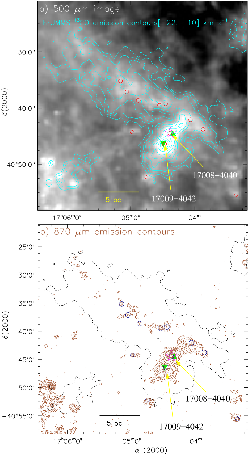
Figure 1.— a) Overlay of the molecular ¹³CO gas on the Herschel image at 500 $\mu$m (size $\sim$0$\arcdeg$.62 $\times$ 0$\arcdeg$.62; central coordinates: $\alpha_{2000}$ = 17^h04^m49.3^s, $\delta_{2000}$ = $-$40$\arcdeg$39$\arcmin$43$\farcs 8$). The ¹³CO emission is integrated over a velocity range of $-$22 to $-$10 km s^-1. The contours of ¹³CO (in cyan) are shown with the levels of 12.5, 16, 20, 26, 32, 40, 52, 64, and 75 K km s^-1. b) Overlay of the molecular ¹³CO gas on the ATLASGAL 870 $\mu$m dust continuum contours. The ATLASGAL dust continuum contours (in brown) are drawn with the levels of 0.13, 0.3, 0.5, 0.8, 1.4, 2.2, 3.4, 5.8, and 11 Jy/beam. The broken contour of ¹³CO (in black) is shown with a level of 12.5 K km s^-1. The positions of the observed ATLASGAL dust clumps at 870 $\mu$m (from Urquhart et al., 2018) are also marked in each figure (see circle and diamond symbols, and also Table 1). Nine clumps highlighted with circles are traced in a velocity range of [-18, -15] km s^-1, while other three clumps marked with diamonds are traced in different V_lsr values (i.e., $-$4.6, $-$26.2, and $-$23.8 km s^-1; see Table 1). In both the panels, the positions of IRAS 17008-4040, IRAS 17009-4042, and 6.7 GHz mme are marked by triangle, upside down triangle, and star, respectively. The scale bar referring to 5 pc (at a distance of 2.4 kpc) is shown in both the panels.

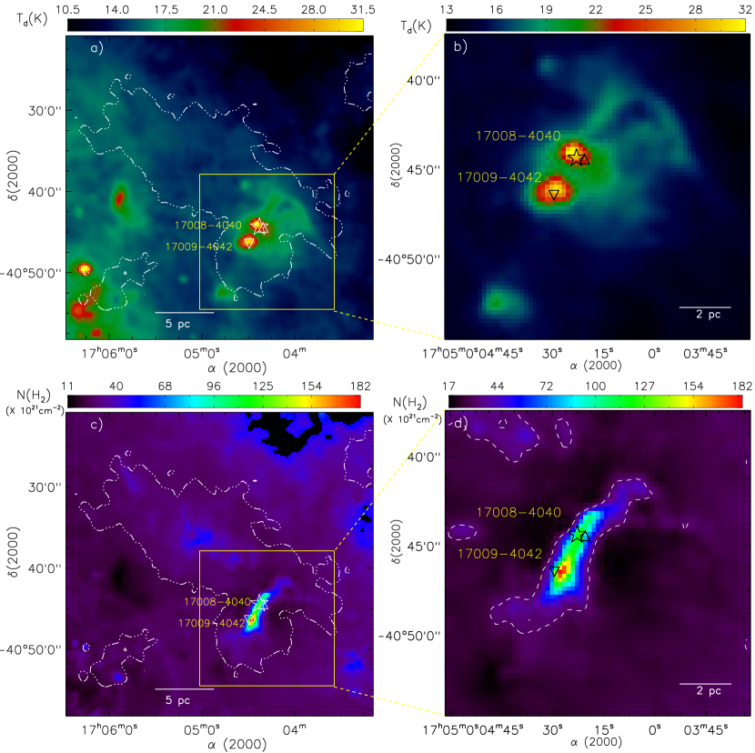
Figure 2.— a) Herschel temperature map (size $\sim$0$\arcdeg$.62 $\times$ 0$\arcdeg$.62; see Figure 1a). b) A zoomed-in version of the Herschel temperature map (see a highlighted solid box in Figure 2a). c) Herschel column density map (size $\sim$0$\arcdeg$.62 $\times$ 0$\arcdeg$.62; see Figure 1a). d) A zoomed-in version of the Herschel column density map (see a highlighted solid box in Figure 2c). A dashed $N(\mathrm{H}_{2})$ contour (in white) with a level of 3.2 $\times$ 10²² cm^-2 is also drawn in the panel “d”. In the panels “a” and “c”, a dotted-dashed contour of ¹³CO (in white) is shown with a level of 12.5 K km s^-1. In all the panels, other symbols are the same as in Figure 1.

Figure 3.— a) Spitzer color-magnitude plot ([3.6] $-$ [24] vs [3.6]) of sources observed in our selected field (see Figure 1a). A broken curve (in blue) helps to separate YSOs against contaminated candidates (such as galaxies and disk-less stars). With the help of dashed lines (in black), one can find YSOs belonging to different evolutionary stages. Symbols “$\Diamond$” and “$\Box$” refer to Flat-spectrum and Class III sources, respectively. b) Spitzer color-color plot ([3.6]$-$[4.5] vs. [5.8]$-$[8.0]) of sources. The PAH-emission-contaminated apertures and Class III sources are shown by “$\times$” (in magenta) and “$\Box$” (in cyan). c) Spitzer color-color plot ([4.5]$-$[5.8] vs [3.6]$-$[4.5]) of sources. An extinction vector (from Flaherty et al., 2007) is also drawn in each panel. In the panels “b” and “c”, the dots refer to the stars with only photospheric emission. In each panel, Class I and Class II YSOs are represented by circles (in red) and triangles (in blue), respectively.

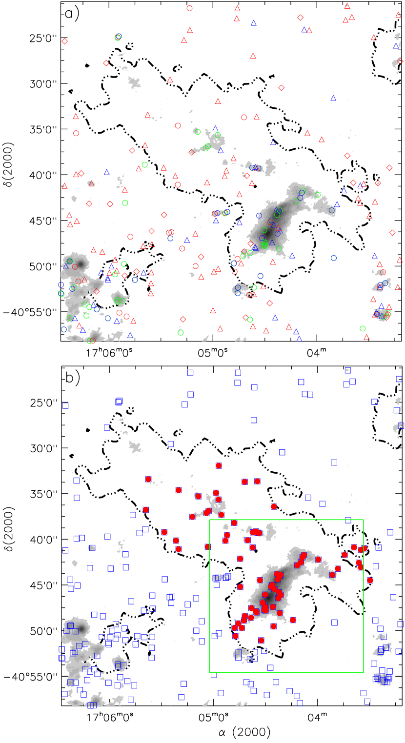
Figure 4.— Spatial distribution of YSOs observed in our selected field (see Figure 1a). a) Overlay of the selected YSOs (Class I (circles), Flat-spectrum (diamond), and Class II (triangles)) on the ¹³CO emission and the ATLASGAL 870 $\mu$m dust continuum contour map (see also Figure 1). The YSOs (in red) are selected using the color-magnitude ([3.6] $-$ [24] vs [3.6]; see Figure 3a), while the YSOs (in blue) identified using the color-color plot ([3.6]$-$[4.5] vs. [5.8]$-$[8.0]; see Figure 3b). The YSOs (in green) are selected using the color-color plot ([4.5]$-$[5.8] vs [3.6]$-$[4.5]; see Figure 3c). b) Filled squares (in red) indicate the YSOs distributed within the molecular cloud boundary, while the YSOs outside the molecular cloud boundary are marked by open squares (in blue).

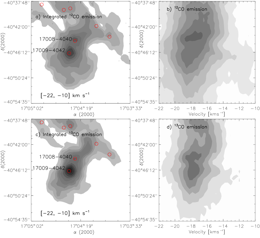
Figure 5.— Distribution of ¹²CO and ¹³CO emission toward the region around IRAS 17008-4040 and IRAS 17009-4042 (see the dotted-dashed box in Figure 4b; size$\sim$16$\farcm 8$ $\times$ 16$\farcm 8$; centered at $\alpha_{2000}$ = 17^h04^m17.7^s, $\delta_{2000}$ = $-$40$\arcdeg$46$\arcmin$14$\farcs 4$). The contour maps of integrated ¹²CO emission (see top left panel “a”) and ¹³CO (see bottom left panel “c”) emission in a velocity range of $-$22 to $-$10 km s^-1. Declination-velocity maps of ¹²CO (see top right panel “b”) and ¹³CO (see bottom right panel “d”). In the panel “a”, the contour levels of ¹²CO are 30, 35, 40, 50, 60, 70, 80, and 90% of the peak value (i.e. 190.86 K km s^-1). In the panel “c”, the contour levels of ¹³CO are 20, 25, 30, 35, 40, 50, 60, 70, 80, and 90% of the peak value (i.e. 92.75 K km s^-1). The ATLASGAL dust continuum clumps at 870 $\mu$m (from Urquhart et al., 2018) are also overlaid on each molecular intensity map (see panels “a” and “c”).

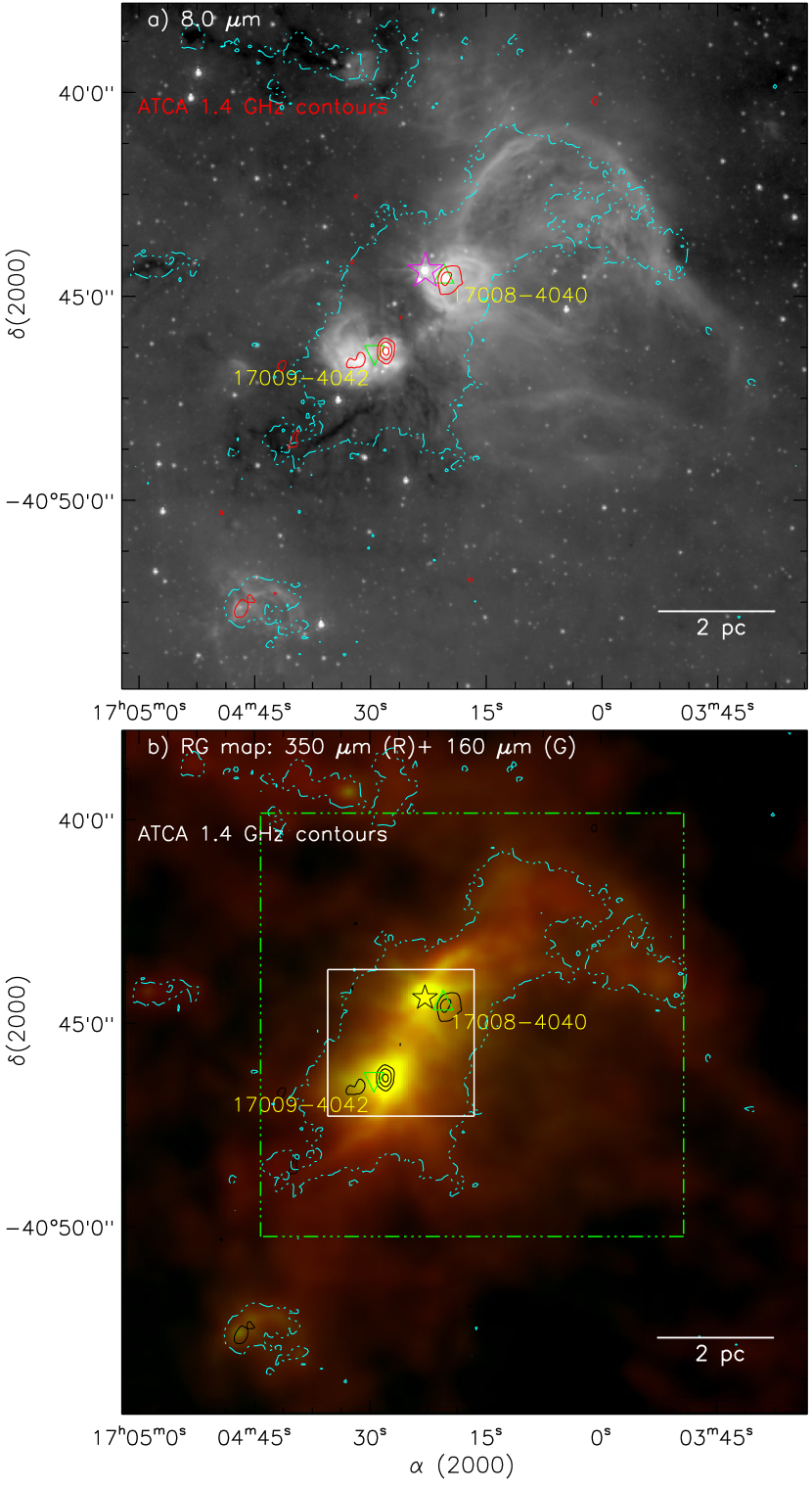
Figure 6.— a) Overlay of the ATLASGAL 870 $\mu$m dust continuum contour (in cyan) and the ATCA 1.4 GHz continuum contours (in red; angular resolution $\sim$10^′′.1 $\times$ 6^′′.1; Garay et al., 2006) on the Spitzer 8.0 $\mu$m image (see the dotted-dashed box in Figure 3b). b) Overlay of the ATLASGAL 870 $\mu$m dust continuum contour (in cyan) and the ATCA 1.4 GHz continuum contours (in black) on a two color-composite map. The color-composite map is the result of the combination of two bands: 350 $\mu$m (red) and 160 $\mu$m (green). In each panel, the ATLASGAL 870 $\mu$m dust continuum contour is drawn with a level of 0.13 Jy/beam, and the ATCA 1.4 GHz continuum contours are shown with the levels of 3.96, 39.59, and 237.53 mJy/beam. Other symbols are the same as in Figure 1.

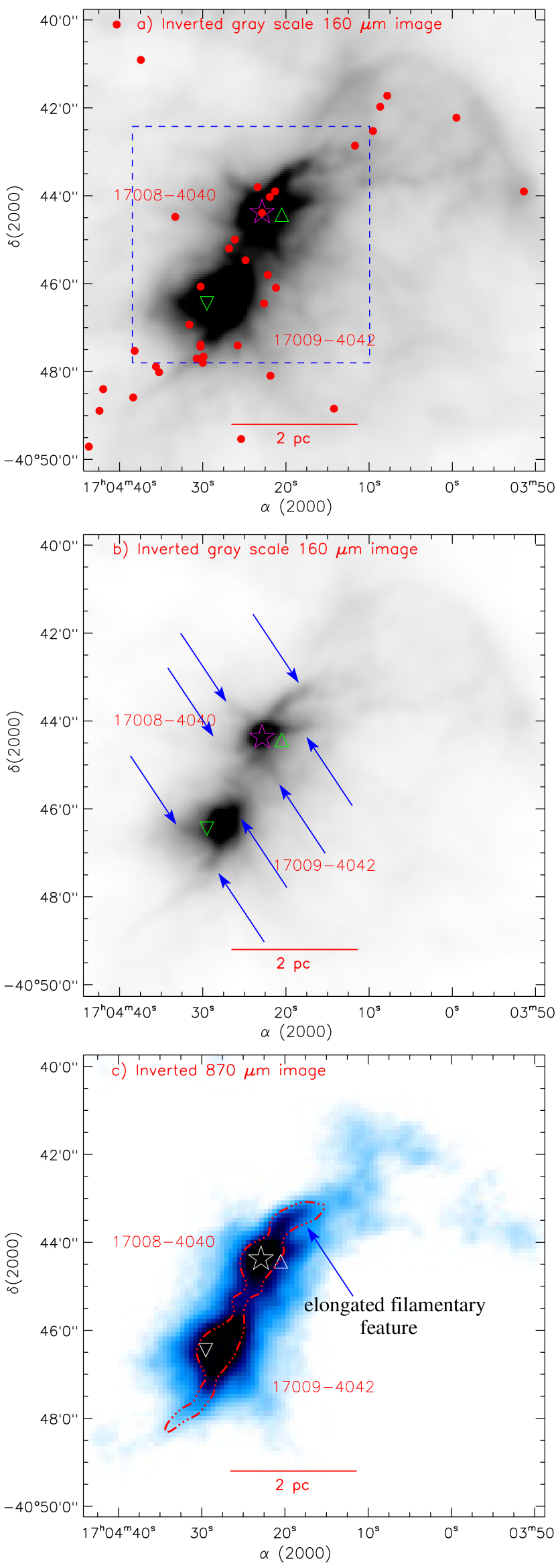
Figure 7.— a) Overlay of the selected YSOs (red filled circles) on an inverted gray scale Herschel 160 $\mu$m image (see the dotted-dashed box in Figure 6b). These YSOs are distributed within the molecular cloud boundary, and are taken from Figure 4b. b) The panel displays an inverted gray scale Herschel 160 $\mu$m image (resolution $\sim$12^′′). The embedded faint filament-like features are also highlighted by blue arrows. c) The panel displays an inverted ATLASGAL 870 $\mu$m image (beam size $\sim$19^′′.2). An elongated filamentary feature is highlighted by a broken contour (in red). In each panel, other symbols are the same as in Figure 1.

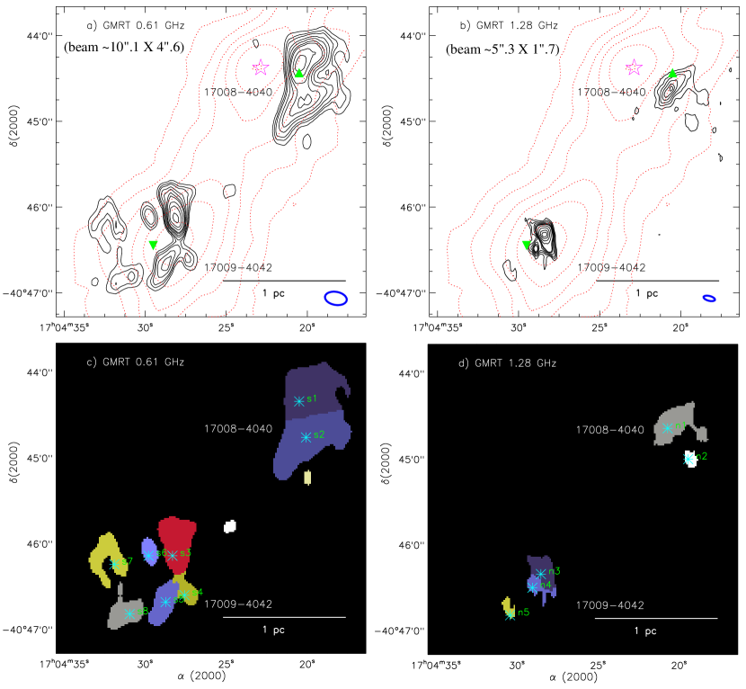
Figure 8.— High-resolution radio continuum maps at two GMRT frequencies toward IRAS 17008-4040 and IRAS 17009-4044 (see the solid box in Figure 6b). a) GMRT 0.61 GHz continuum contours (in black; beam size $\sim$10^′′.1 $\times$ 4^′′.6; sensitivity $\sim$0.3 mJy/beam) are shown with the levels of 1.48, 2.5, 3.5, 5.5, 7.5, 10, 12, 17, 22, and 28 mJy/beam. b) GMRT 1.28 GHz continuum contours (in black; beam size $\sim$5^′′.3 $\times$ 1^′′.7; sensitivity $\sim$0.4 mJy/beam) are shown with the levels of 3.5, 6.5, 9.5, 13, 16, 18, 25, 35, 45, and 52 mJy/beam. c–d) The boundary of each identified clump in both the GMRT radio maps is highlighted along with its corresponding clump ID (see Table 3 and also Figures 8a and 8b). In the panels “a” and “b”, the ATLASGAL 870 $\mu$m dust continuum contours (in red) are displayed with the levels of 0.8, 1.4, 2.2, 3.4, 5.8, and 11 Jy/beam, and a star symbol indicates the position of the 6.7 GHz mme. Ellipses (in blue) represent the beam sizes of radio continuum data in the panels “a” and “b”. In all the panels, other symbols are the same as in Figure 1.

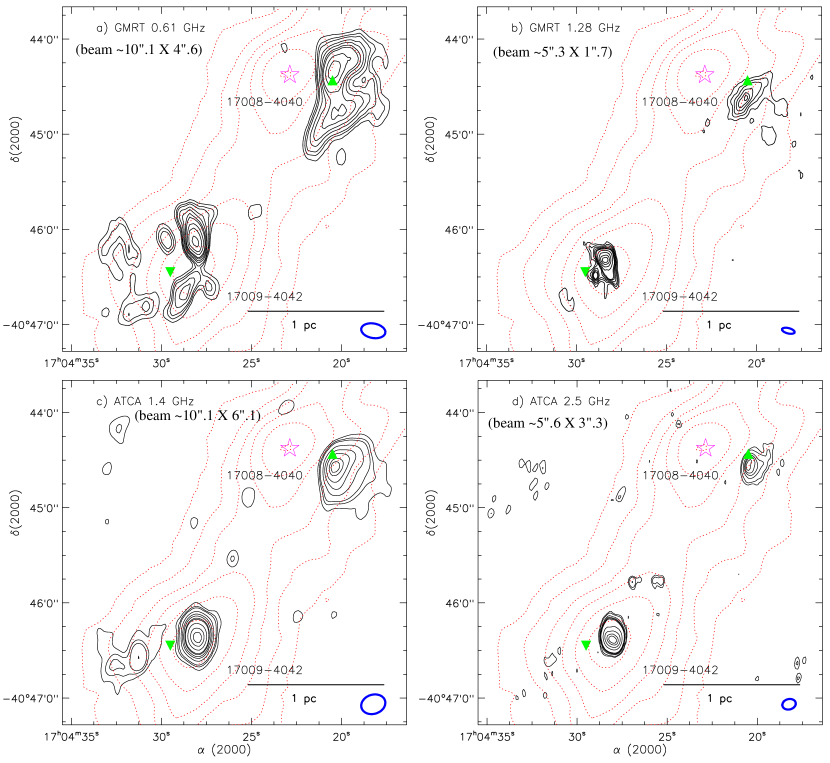
Figure 9.— Radio continuum emission contours at different frequencies toward IRAS 17008-4040 and IRAS 17009-4044 (see the solid box in Figure 6b). a) GMRT 0.61 GHz continuum contours (see Figure 8a). b) GMRT 1.28 GHz continuum contours (see Figure 8b). c) ATCA 1.4 GHz continuum contours (in black; beam size $\sim$10^′′.1 $\times$ 6^′′.1) are shown with the levels of 2, 4, 6, 15, 28, 43, 66, 80, 150, 250, and 340 mJy/beam (see also Garay et al., 2006). d) ATCA 2.5 GHz continuum contours (in black; beam size $\sim$5^′′.6 $\times$ 3^′′.3) are shown with the levels of 1.6, 2.6, 6.2, 9.5, 12, 15, 60, 140, 250, and 330 mJy/beam (see also Garay et al., 2006). In each panel, the ATLASGAL 870 $\mu$m dust continuum contours (in red) are displayed with the levels of 0.8, 1.4, 2.2, 3.4, 5.8, and 11 Jy/beam. In all the panels, ellipses (in blue) represent the beam sizes of radio continuum data. In each panel, a star symbol indicates the position of the 6.7 GHz mme. In all the panels, other symbols are the same as in Figure 1.

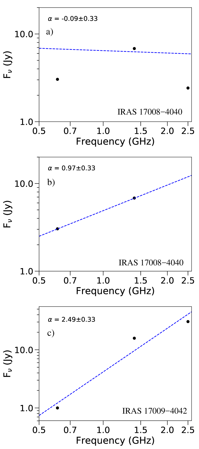
Figure 10.— a) Radio spectral index plot of the radio clump associated with IRAS 17008-4040. Filled circles (in black) are the flux densities at 0.61, 1.4, and 2.5 GHz. b) Same as Figure 10a, but only two flux densities at 0.61 and 1.4 GHz are considered. c) Radio spectral index plot of the radio clump associated with IRAS 17009-4042. Filled circles (in black) are the flux densities at 0.61, 1.4, and 2.5 GHz.

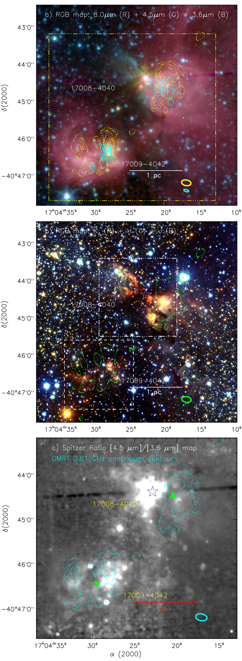
Figure 11.— a) Overlay of the GMRT 0.61 GHz continuum contours (in orange) and 1.28 GHz continuum contours (in cyan) on a three color-composite map (see the dashed box in Figure 7a and also Figure 8). The color-composite map is the result of the combination of three bands: 8.0 $\mu$m (red), 4.5 $\mu$m (green), and 3.6 $\mu$m (blue). b) Overlay of the GMRT 0.61 GHz continuum contour (in green; see also Figure 8) on a three color-composite map (see the dashed box in Figure 7a). The color-composite map is the result of the combination of three VVV bands: K_s (red), H (green), and J $\mu$m (blue). The dotted-dashed box (in white) encompasses the area shown in Figure 13a, while the dashed box (in white) refers the area shown in Figure 13b. c) Overlay of the GMRT 0.61 GHz contours (in cyan) on the Spitzer ratio map of 4.5 $\mu$m/3.6 $\mu$m emission (see the dotted-dashed box in Figure 11a and also Figure 8). The ratio map is exposed to a Gaussian smoothing function with a width of 4 pixels. In each panel, a star symbol indicates the position of the 6.7 GHz mme. An infrared counterpart (IRc) of the 6.7 GHz mme (i.e. IRcmme) is seen in each color-composite map, and is found to be away from the radio continuum emission. In each panel, other symbols are the same as in Figure 1. Ellipses represent the beam sizes of radio continuum data in the panels.

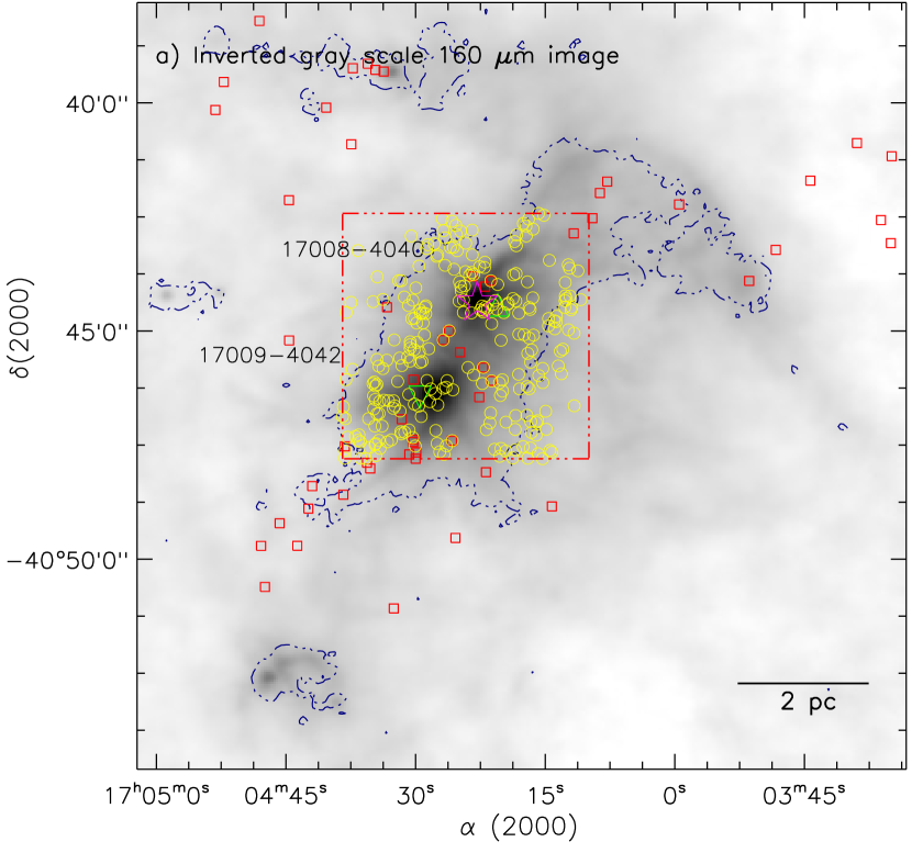
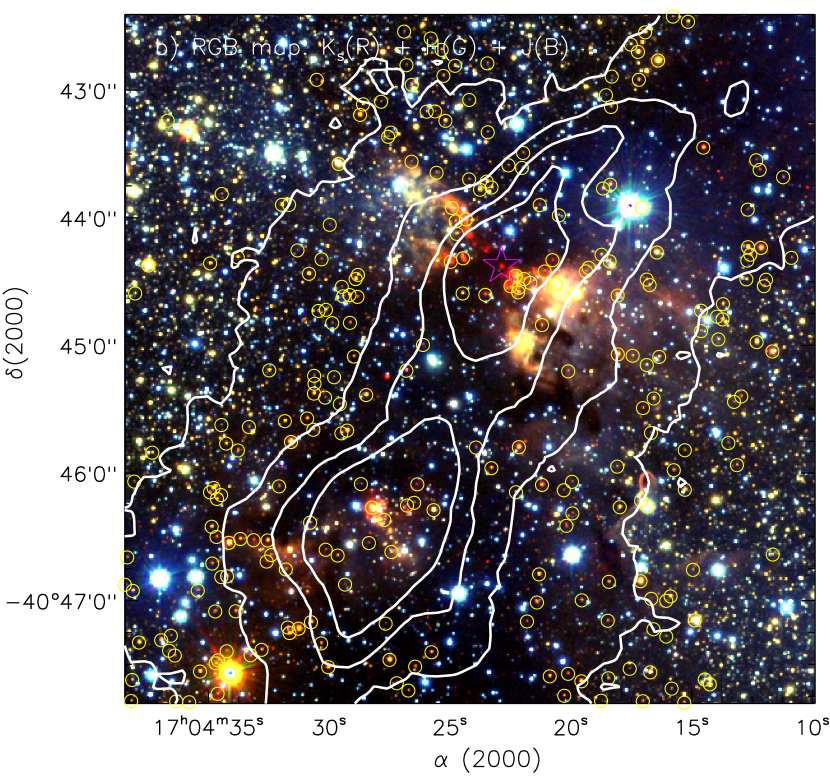
Figure 12.— a) Overlay of the infrared-excess sources and the ATLASGAL 870 $\mu$m emission contour on an inverted gray scale Herschel 160 $\mu$m image. The ATLASGAL 870 $\mu$m dust continuum contour (in navy) is drawn with a level of 0.13 Jy/beam. The YSOs distributed within the molecular cloud boundary are highlighted with open squares (in red) are taken from Figure 4b. The sources with H$-$K_s $>$ 1.8 are shown by yellow circles, and are selected only for an area enclosed within a dotted-dashed box (see also Figure 12b). The dotted-dashed box (in red) encompasses the area shown in Figure 12b. b) Overlay of the sources with H$-$K_s $>$ 1.8 (see yellow circles) and the ATLASGAL 870 $\mu$m dust continuum contours on the VVV NIR color-composite map. The color-composite map is the same as in Figure 11b. The ATLASGAL 870 $\mu$m contours (in white) are shown with the levels of 0.13, 0.8, 1.8, and 3 Jy/beam. In each panel, other symbols are the same as in Figure 1.

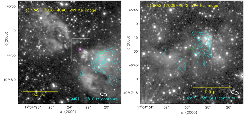
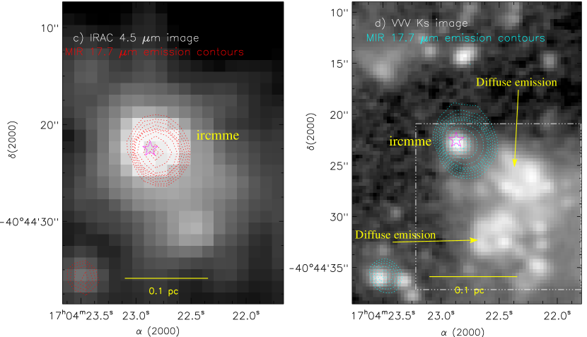
Figure 13.— a) Overlay of the GMRT 1.28 GHz continuum contours (in cyan) on the VVV K_s image toward IRAS 17008-4040 (see the dotted-dashed box in Figure 11b). The contour levels are 3.5, 6.5, 9.5, 13, and 17 mJy/beam. The solid box (in white) encompasses the area shown in Figures 13c and 13d. b) Overlay of the GMRT 1.28 GHz continuum contours (in cyan) on the VVV K_s image toward IRAS 17009-4042 (see the dashed box in Figure 11b). The contour levels are 3.5, 13, 25, and 45 mJy/beam. c) Overlay of the TIMMI2 MIR emission contours at 17.7 $\mu$m (in red; resolution $\sim$1^′′; Morales et al., 2009) on the Spitzer 4.5 $\mu$m map (see the solid box in Figure 13a). d) Overlay of the TIMMI2 MIR emission contours at 17.7 $\mu$m (in cyan) on the VVV K_s image (see the solid box in Figure 13a). The dotted-dashed box (in white) encompasses the area shown in Figures 14a and 14b. Ellipses (in white) represent the beam sizes of radio continuum data in the panels “a” and “b”. In the panels “c” and “d”, the TIMMI2 MIR 17.7 $\mu$m data are taken from Morales et al. (2009). In all the panels, other symbols are the same as in Figure 1.

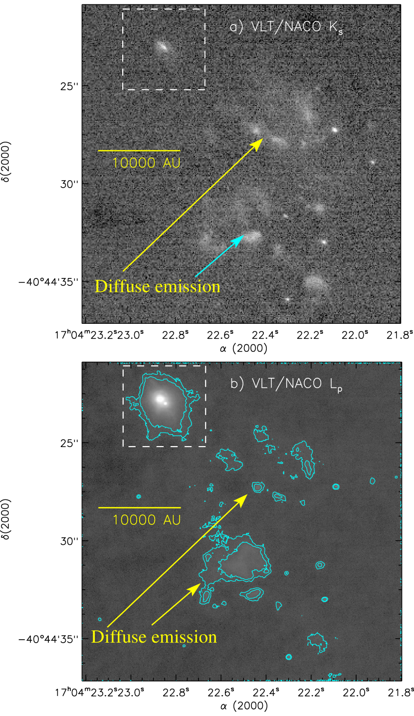
Figure 14.— The VLT/NACO adaptive-optics K_s-band (a) and L^′-band (b) images of the region toward the source “IRcmme” (see the dotted-dashed box in Figure 13d). In the panel “b”, L^′ contours (in cyan) are also shown to highlight the faint features.

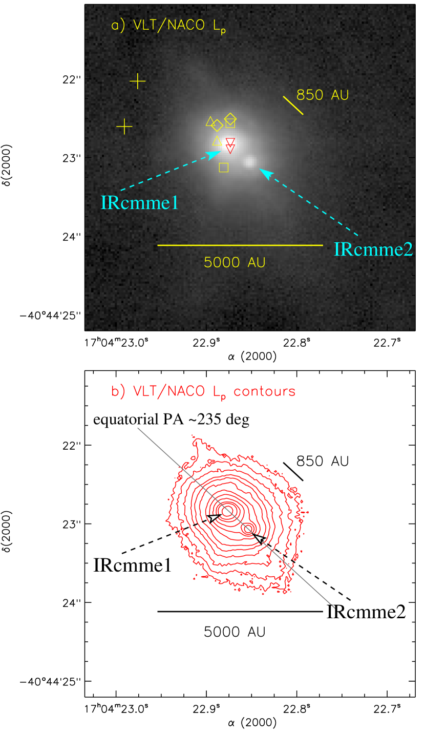
Figure 15.— a) A zoomed-in view of the source “IRcmme” using the VLT/NACO L^′ image (see the dashed box in Figures 14a and 14b). Ten positions of the 6.7 GHz maser spots (from Walsh et al., 1998) are marked by plus symbols (V_lsr range = [$-$14, $-$15] km s^-1), diamonds (V_lsr range = [$-$15, $-$17] km s^-1), triangles (V_lsr range = [$-$18, $-$19] km s^-1), squares (V_lsr range = [$-$19, $-$20] km s^-1), and upside down triangles (V_lsr range = [$-$20, $-$22.5] km s^-1). b) A zoomed-in view of the source “IRcmme” using the VLT/NACO L^′ emission contours (see the dashed box in Figures 14a and 14b). The NACO L^′ image has resolved the source “IRcmme” into two point-like sources (i.e. IRcmme1 and IRcmme2), which are embedded in an extended envelope within a scale of 5000 AU. The separation between “IRcmme1” and “IRcmme2” is $\sim$900 AU.

Table 1ATLASGAL 870 $\mu$m dust continuum clumps from Urquhart et al. (2018) in our selected target field (see Figure 1a). We have listed ID, equatorial coordinates, 870 $\mu$m peak flux density (P₈₇₀), 870 $\mu$m integrated flux density (S₈₇₀), radial velocity (V_lsr), distance, clump effective radius ($R_{\mathrm{c}}$), dust temperature ($T_{\mathrm{d}}$), and clump mass ($M_{\mathrm{clump}}$). The positions of IRAS 17008-4040 and IRAS 17009-4042 are embedded in the clumps c1 and c2, respectively. In Figures 1a and 1b, three clumps (i.e. c10, c11, and c12) are highlighted by diamonds, while nine clumps (i.e. c1–c9) are shown by circles.

ID	RA	DEC	P870	S870	Vlsr	distance	Rc	Td	log$M_{\mathrm{clump}}$
	(J2000)	(J2000)	(Jy/beam)	(Jy)	(km s-1)	(kpc)	(pc)	(K)	($M_{\odot}$)
c1	17:04:23.10	-40:44:26.72	11.69	133.92	-17.0	2.4	3.04	30.0	3.386
c2	17:04:28.33	-40:46:24.61	17.27	143.50	-17.3	2.4	2.15	27.3	3.463
c3	17:03:52.34	-40:43:45.94	0.46	7.72	-16.9	2.4	0.64	21.9	2.325
c4	17:04:04.03	-40:42:03.59	0.62	14.43	-15.8	2.4	1.14	16.5	2.781
c5	17:04:27.33	-40:39:14.66	0.39	3.44	-17.4	2.4	0.28	16.5	2.159
c6	17:04:33.13	-40:39:28.90	0.52	4.76	-16.7	2.4	0.28	25.2	2.031
c7	17:04:52.85	-40:38:38.11	0.40	0.71	-17.3	2.4	0.28	14.2	1.580
c8	17:05:03.72	-40:37:06.83	0.36	1.99	-17.6	2.4	0.28	13.5	2.065
c9	17:05:09.54	-40:35:09.92	0.45	0.92	-16.3	2.4	0.28	13.8	1.713
c10	17:04:45.40	-40:52:16.13	0.64	3.72	-4.6	2.4	0.47	23.9	1.955
c11	17:04:59.09	-40:44:12.72	0.37	2.04	-26.2	2.4	0.28	14.2	2.039
c12	17:03:21.40	-40:55:32.00	0.66	4.47	-23.8	2.4	0.92	13.4	2.422

Table 2List of several surveys used in this paper.

Survey	Wavelength/Frequency	Resolution ($\arcsec$)	Reference
Giant Metre-wave Radio Telescope (GMRT) archival data	0.61, 1.28 GHz	$<$10	Proposal-ID: 11SKG01
Three-mm Ultimate Mopra Milky Way Survey (ThrUMMS)	115.27, 110.2 GHz	$\sim$72	Barnes et al. (2015)
APEX Telescope Large Area Survey of the Galaxy (ATLASGAL)	870 $\mu$m	$\sim$19.2	Schuller et al. (2009)
Herschel Infrared Galactic Plane Survey (Hi-GAL)	70, 160, 250, 350, 500 $\mu$m	$\sim$5.8–37	Molinari et al. (2010)
Spitzer Galactic Legacy Infrared Mid-Plane Survey Extraordinaire (GLIMPSE)	3.6, 4.5, 5.8, 8.0 $\mu$m	$\sim$2	Benjamin et al. (2003)
ESO 8.2m Very Large Telescope (VLT) adaptive-optics near-infrared archival data	2.18, 3.8 $\mu$m	$\sim$0.2, $\sim$0.1	Proposal-ID: 083.C-0582(A)
Vista Variables in the Vía Líactea (VVV)	1.25–2.2 $\mu$m	$\sim$0.8	Minniti et al. (2010)
Two Micron All Sky Survey (2MASS)	1.25–2.2 $\mu$m	$\sim$2.5	Skrutskie et al. (2006)

Table 3Physical properties of the ionized clumps observed in the GMRT 0.61 and 1.28 GHz radio continuum maps. Table provides ID, equatorial coordinates, deconvolved effective radius of the ionized clump ($R_{\mathrm{HII}}$), total flux (S_ν), Lyman continuum photons (log$N_{\mathrm{uv}}$), and radio spectral type. Eight ionized clumps (s1–s8) are identified in the GMRT 0.61 GHz radio map (see Figure 8c), while five radio sources (n1–n5) are traced in the GMRT 1.28 GHz radio map (see Figure 8d).

ID	RA	Dec	$R_{\mathrm{HII}}$	Sν	log$N_{\mathrm{uv}}$	Spectral Type	Frequency
	(J2000)	(J2000)	(pc)	(Jy)	(s-1)		(GHz)
s1	17:04:20.5	$-$40:44:20.5	0.24	0.220	46.96	B0V–O9.5V	0.61
s2	17:04:20.1	$-$40:44:45.7	0.25	0.170	46.85	B0V–O9.5V	0.61
s3	17:04:28.3	$-$40:46:08.5	0.18	0.138	46.76	B0V–O9.5V	0.61
s4	17:04:27.6	$-$40:46:36.1	0.10	0.011	45.68	B1V–B0.5V	0.61
s5	17:04:28.7	$-$40:46:40.9	0.14	0.036	46.17	B1V–B0.5V	0.61
s6	17:04:29.8	$-$40:46:08.5	0.09	0.010	45.60	B1V–B0.5V	0.61
s7	17:04:32.0	$-$40:46:14.5	0.15	0.024	45.99	B1V–B0.5V	0.61
s8	17:04:31.0	$-$40:46:49.3	0.14	0.019	45.91	B1V–B0.5V	0.61
n1	17:04:20.7	$-$40:44:38.5	0.16	0.482	47.33	B0.5V–B0V	1.28
n2	17:04:19.4	$-$40:45:00.1	0.06	0.039	46.25	B1V–B0.5V	1.28
n3	17:04:28.5	$-$40:46:20.5	0.12	0.638	47.46	B0.5V–B0V	1.28
n4	17:04:29.0	$-$40:46:30.1	0.08	0.140	46.80	B0.5V–B0V	1.28
n5	17:04:30.4	$-$40:46:49.3	0.06	0.039	46.25	B1V–B0.5V	1.28

References

- Barnes et al. (2015) Barnes,P., Muller,E., & Indermuehle, B. 2015, ApJ, 812, 6
- Baug et al. (2015) Baug, T., Ojha, D. K., Dewangan, L. K., et al. 2015, MNRAS, 454, 4335
- Baug et al. (2018) Baug, T., Dewangan, L. K., Ojha, D. K., et al. 2018, ApJ, 852, 119
- Benjamin et al. (2003) Benjamin, R. A.,Churchwell, E., Babler, B. L., et al. 2003, PASP, 115, 953
- Bohlin et al. (1978) Bohlin, R. C., Savage, B. D., & Drake, J. F. 1978, ApJ, 224, 13233
- Cesaroni et al. (2017) Cesaroni, R., Sánchez-Monge, Á., Beltrán, M. T., et al. 2017, A&A, 602, 59
- Cyganowski et al. (2008) Cyganowski, C. J., Whitney, B. A., Holden, E., et al. 2017, AJ, 136, 2391
- de Villiers et al. (2015) de Villiers, H. M., Chrysostomou, A., Thompson, M. A., et al. 2015, MNRAS, 449, 119
- Dewangan et al. (2015a) Dewangan, L. K., Mayya, Y. D., Luna, A., & Ojha, D. K. 2015a, ApJ, 803, 100
- Dewangan et al. (2015b) Dewangan, L. K., Luna, A., Ojha, D. K., et al. 2015b, ApJ, 811, 79
- Dewangan et al. (2016a) Dewangan, L. K., Ojha, D. K., Luna, A., et al. 2016a, ApJ, 819, 66
- Dewangan et al. (2016b) Dewangan, L. K., Ojha, D. K., Zinchenko, I., et al. 2016b, ApJ, 833, 246
- Dewangan et al. (2017a) Dewangan, L. K., Ojha, D. K., Zinchenko, I., Janardhan, P., & Luna, A. 2017a, ApJ, 834, 22
- Dewangan et al. (2017b) Dewangan, L. K., Ojha, D. K., & Baug, T. 2017b, ApJ, 844, 15
- Dewangan et al. (2018) Dewangan, L. K., Devaraj, R., & Ojha, D. K. 2018, ApJ, 854, 106
- Flaherty et al. (2007) Flaherty, K. M., Pipher, J. L., Megeath, S. T., et al. 2007, ApJ, 663, 1069
- Garay et al. (2006) Garay, G., Brooks, K. J., Mardones, D., & Norris, R. P. 2006, ApJ, 651, 914
- Garay et al. (2007) Garay, G., Mardones, D., Brooks, K. J., Videla, L., & Contreras, Y. 2007, ApJ, 666, 309
- Getman et al. (2007) Getman, K. V., Feigelson, E. D., Garmire,G., Broos, P., & Wang, J. 2007, ApJ, 654, 316
- Guieu et al. (2010) Guieu, S., Rebull, L. M., Stauffer, J. R., et al. 2010, ApJ, 720, 46
- Gutermuth et al. (2009) Gutermuth, R. A., Megeath, S. T., Myers, P. C., et al. 2009, ApJS, 184, 18
- Gutermuth & Heyer (2015) Gutermuth, R. A., & Heyer,M. 2015, AJ, 149, 64
- Hartmann et al. (2005) Hartmann, L., Megeath, S. T., Allen, L., et al. 2005, ApJ, 629, 881
- Hennemann et al. (2012) Hennemann, M., Motte, F., Schneider, N., et al. 2012, A&A, 543, 3
- Indebetouw et al. (2005) Indebetouw, R., Mathis, J. S., Babler, B. L., et al. 2005, ApJ, 619, 931
- Kirk et al. (2013) Kirk, H., Myers, P. C., Bourke, T. L., et al. 2013, ApJ, 766, 115
- Kratter et al. (2008) Kratter, K. M., Matzner, C. D., & Krumholz, M. R. 2008, ApJ, 681, 375
- Krumholz & Thompson (2007) Krumholz, M. R., & Thompson, T. A. 2007, ApJ, 661, 1034
- Lada et al. (2006) Lada, C. J., Muench, A. A., Luhman, K. L., et al. 2006, AJ, 131, 1574
- Lenzen et al. (2003) Lenzen, R., Hartung, M., Brandner, W., et al. 2003, Proc. SPIE, 4841, 944
- Liu et al. (2012) Liu, H. B., Quintana-Lacaci, G., Wang, K., et al. 2012, ApJ, 745, 61
- Liu et al. (2016) Liu, T., Zhang, Q., Kim, K.-T., et al. 2016, ApJ, 824, 31
- Mallick et al. (2012) Mallick, K. K., Ojha, D. K., Samal, M. R., et al. 2012, ApJ, 759, 48
- Mallick et al. (2013) Mallick, K. K., Kumar, M. S. N., Ojha, D. K., et al. 2013, ApJ, 779, 113
- Mallick et al. (2015) Mallick, K. K., Ojha, D. K., Tamura, M., et al. 2015, MNRAS, 447, 2307
- Matsakis et al. (1976) Matsakis, D. N., Evans, N. J., II, Sato, T., & Zuckerman, B. 1976, AJ, 81, 172
- MacLaren et al. (1988) MacLaren, I., Richardson, K. M., & Wolfendale, A. W. 1988, ApJ, 333, 821
- Minier et al. (2001) Minier, V., Conway, J. E., & Booth, R. S. 2001, A&A, 369, 278
- Minniti et al. (2010) Minniti, D.; Lucas, P. W.; Emerson, J. P., et al. 2010, NewA, 15, 433
- Minniti et al. (2017) Minniti, D., Lucas, P., & VVV Team. 2017, VizieR Online Data Catalog, 2348
- Molinari et al. (2010) Molinari, S., Swinyard, B., Bally, J., et al., 2010, A&A, 518, L100
- Morales et al. (2009) Morales, E. F. E., Mardones, D., Garay, G., Brooks, K. J., Pineda, J. E. 2009, ApJ, 698, 488
- Motte et al. (2017) Motte, F., Bontemps, S., & Louvet, F. 2017, arXiv:1706.00118
- Myers (2009) Myers, P. C. 2009, ApJ, 700, 1609
- López et al. (2011) López, C., Bronfman, L., Nyman, L.-Å., May, J., & Garay, G. 2011, 534, 131
- Panagia (1973) Panagia, N. 1973, AJ, 78, 929
- Peretto et al. (2013) Peretto, N., Fuller, G.‘A., Duarte-Cabral, A., et al. 2013, A&A, 555, 112
- Rebull et al. (2011) Rebull, L. M., Guieu, S., Stauffer, J. R., et al. 2011, ApJS, 193, 25
- Robitaille et al. (2008) Robitaille T. P., Meade, M. R., Babler, B. L., et al. 2008, AJ, 136, 2413
- Rousset et al. (2003) Rousset, G., Lacombe, F., Puget, P., et al. 2003, Proc. SPIE, 4839, 140
- Saito et al. (2012) Saito, R. K., Hempel, M., Minniti, D., et al. 2012, A&A, 537, A107
- Schuller et al. (2009) Schuller, F., Menten, K. M., Contreras, Y., et al. 2009, A&A, 504, 415
- Schneider et al. (2012) Schneider, N., Csengeri, T., Hennemann, M., et al. 2012, A&A, 540, L11
- Skrutskie et al. (2006) Skrutskie, M. F., Cutri, R. M., Stiening, R., et al. 2006, AJ, 131, 1163
- Stanimirovic (2002) Stanimirovic, S., 2002, ASPC, 278, 375
- Takakuwa et al. (2017) Takakuwa, S., Saigo, K., Matsumoto, T., et al. 2017, ApJ, 837, 86
- Tan et al. (2014) Tan, J. C., Beltrán, M. T., Caselli, P., et al. 2014, in Protostars and Planets VI, ed. H. Beuther et al. (Tucson, AZ: Univ. Arizona Press), 149
- Thompson et al. (2001) Thompson, A. R, Moran, J. M., Swenson, G. W. 2001, Interferometry and Synthesis in Radio Astronomy New York, NY: Wiley-Interscience
- Tobin et al. (2016) Tobin, J. J., Looney, L. W., Li, Zhi-Yun, et al. 2016, ApJ, 818, 73
- Urquhart et al. (2013) Urquhart, J. S., Moore, T. J. T., Schuller, F., et al. 2013, MNRAS, 431, 1752
- Urquhart et al. (2018) Urquhart, J. S., König, C., Giannetti, A., et al. 2018, MNRAS, 437, 1059
- Yan et al. (2016) Yan, Q. Z., Xu, Y., Zhang, B., et al. 2016, AJ, 152, 117
- Yang et al. (2018) Yang, A. Y., Thompson, M. A., Tian, W. W., et al. 2018 arXiv:1809.00404
- Yuan et al. (2018) Yuan, J., Li, Jin-Zeng, Wu, Y., et al. 2018, ApJ, 852, 12
- Walsh et al. (1998) Walsh, A. J., Burton, M. G., Hyland, A. R., & Robinson, G. 1998, MNRAS, 301, 640
- Williams et al. (2018) Williams, G. M., Peretto, N., Avison, A., Duarte-Cabral, A., & Fuller, G. 2018 arXiv:1801.07253
- Zinnecker & Yorke (2007) Zinnecker, H., & Yorke, H. W. 2007, ARA&A, 45, 481