Fibrations of 3-manifolds and asymptotic translation length in the arc complex

Abstract.

Given a 3-manifold $M$ fibering over the circle, we investigate how the asymptotic translation lengths of pseudo-Anosov monodromies in the arc complex vary as we vary the fibration. We formalize this problem by defining normalized asymptotic translation length functions $\mu_{d}$ for every integer $d\geq 1$ on the rational points of a fibered face of the unit ball of the Thurston norm on $H^{1}(M;\mathbb{R})$. We show that even though the functions $\mu_{d}$ themselves are typically nowhere continuous, the sets of accumulation points of their graphs on $d$-dimensional slices of the fibered face are rather nice and in a way reminiscent of Fried’s convex and continuous normalized stretch factor function. We also show that these sets of accumulation points depend only on the shape of the corresponding slice. We obtain a particularly concrete description of these sets when the slice is a simplex. We also compute $\mu_{1}$ at infinitely many points for the mapping torus of the simplest hyperbolic braid to show that the values of $\mu_{1}$ are rather arbitrary. This suggests that giving a formula for the functions $\mu_{d}$ seems very difficult even in the simplest cases.

1. Introduction

To every fibration $M\to S^{1}$ of a 3-manifold $M$ over the circle, there is an associated element of $H^{1}(M;\mathbb{Z})$, the pullback of a generator of $H^{1}(S^{1};\mathbb{Z})\cong\mathbb{Z}$. The integral cohomology classes that correspond to fibrations of $M$ are organized by the faces of the unit ball of the Thurston norm $\left\|\cdot\right\|$ on $H^{1}(M;\mathbb{R})$ [Thu86]: a face $\mathcal{F}$ can be fibered, in which case every integral point in the interior of the cone $\mathbb{R}_{+}\mathcal{F}$ corresponds to a fibration, or not fibered, in which case no integral point in $\mathbb{R}_{+}\mathcal{F}$ corresponds to a fibration.

An element $\phi\in H^{1}(M;\mathbb{Z})$ is primitive if it cannot be written in the form $k\phi^{\prime}$ for some $\phi^{\prime}\in H^{1}(M;\mathbb{Z})$ and integer $k\geq 2$. If an element $\phi\in H^{1}(M;\mathbb{Z})$ corresponds to a fibration, then it is primitive if and only if the fibers are connected. For any $\phi\in H^{1}(M;\mathbb{Q})$, denote by $\bar{\phi}\in H^{1}(M;\mathbb{Z})$ the unique primitive integral point on the ray $\mathbb{R}_{+}\phi$.

We can now state a classical result of Fried from 1982, which was the main motivation for this work. If $M$ admits a complete finite-volume hyperbolic metric, then the monodromies of the fibrations are pseudo-Anosov mapping classes by Thurston’s Hyperbolization Theorem [Ota96]. For a fibered face $\mathcal{F}$ of $M$, define the normalized entropy function

$$\xi\colon\thinspace\operatorname{int}(\mathcal{F})\cap H^{1}(M;\mathbb{Q})\to\mathbb{R}_{+}$$

by the formula

(1.1) $$\xi(\phi)=\left\|\bar{\phi}\right\|\cdot\log{\lambda(\bar{\phi})}$$

where $\lambda(\bar{\phi})$ denotes the stretch factor of the pseudo-Anosov monodromy corresponding to $\bar{\phi}$. In Theorem E of [Fri82a], Fried proves that the function $\xi$ extends to a convex, continuous function to the interior of $\mathcal{F}$ and $\xi(\phi)\to\infty$ as $\phi\to\partial\mathcal{F}$. The goal of this paper is to investigate analogous functions on the rational points of the fibered faces that are defined not in terms of the stretch factor but another numerical invariant of pseudo-Anosov maps, the asymptotic translation length in the arc complex.

The arc complex $\mathcal{A}(S)$ of a connected punctured surface $S$ is a simplicial complex whose vertices are isotopy classes of properly embedded arcs in $S$ and whose simplices correspond to collections of disjoint arcs. For two vertices $\alpha$ and $\beta$ of $\mathcal{A}(S)$, their distance $d_{\mathcal{A}}(\alpha,\beta)$ is defined as the minimal number of edges of a path in the 1-skeleton of $\mathcal{A}(S)$ that starts at $\alpha$ and ends at $\beta$. The asymptotic translation length of a mapping class $f$ in the arc complex is defined as

$$\ell_{\mathcal{A}}(f)=\liminf_{n\to\infty}\frac{d_{\mathcal{A}}(\alpha,f^{n}(\alpha))}{n}$$

where $\alpha$ is any arc. The number $\ell_{\mathcal{A}}(f)$ is a natural invariant encoding geometric information about the 3-manifold $M$: Futer and Schleimer [FS14] showed that it is proportional to the height and area of the boundary of the maximal cusp in $M$.

Based on work of Baik, Shin and Wu [BSW18], we define the $d$-adic normalized asymptotic translation length function

$$\mu_{d}\colon\thinspace\operatorname{int}(\mathcal{F})\cap H^{1}(M;\mathbb{Q})\to\mathbb{R}_{+}$$

by the formula

(1.2) $$\mu_{d}(\phi)=\left\|\bar{\phi}\right\|^{1+\frac{1}{d}}\cdot\ell_{\mathcal{A}}(\bar{\phi})$$

where $\ell_{\mathcal{A}}(\bar{\phi})$ is defined as $\ell_{\mathcal{A}}(f)$ where $f$ is the monodromy of the connected fiber corresponding to $\bar{\phi}$. In order for $\mu_{d}$ to be defined, the fibers of $M$ have to be punctured, so $M$ has to be a cusped 3-manifold. In this paper, we will work under the stronger hypothesis that the fibered face $\mathcal{F}$ is fully-punctured, meaning that the singular set of every pseudo-Anosov monodromy in $\mathbb{R}_{+}\mathcal{F}$ is contained in the set of punctures of the fiber. (If this condition holds for one monodromy in $\mathbb{R}_{+}\mathcal{F}$, then it holds for all.)

A $d$-dimensional slice of a fibered face $\mathcal{F}$ is an intersection $\mathcal{F}\cap\Sigma$ where $\Sigma$ is a $d+1$-dimensional linear subspace of $H^{1}(M;\mathbb{R})$ intersecting the interior of $\mathcal{F}$. The slice is rational if $\Sigma\cap H^{1}(M;\mathbb{Q})$ is dense in $\Sigma$.

Theorem 1.1.

Let $M$ be a connected cusped 3-manifold that admits a complete finite-volume hyperbolic metric. Let $\mathcal{F}$ be a fully-punctured fibered face of the unit ball of the Thurston norm on $H^{1}(M;\mathbb{R})$. Suppose that $1\leq d\leq\dim(H^{1}(M;\mathbb{R}))-1$ and let $\Omega$ be a rational $d$-dimensional slice of $\mathcal{F}$. Consider $\operatorname{Graph}(\mu_{d}|_{\Omega})\subset\Omega\times\mathbb{R}$, the graph of the normalized asymptotic translation length function $\mu_{d}$, restricted to $\Omega$.

There is a continuous function $g\colon\thinspace\operatorname{int}(\Omega)\to\mathbb{R}_{+}$ such that $g(\phi)\to\infty$ as $\phi\to\partial\Omega$ and the set of accumulation points of $\operatorname{Graph}(\mu_{d}|_{\Omega})$ is

$$\{(\omega,g(\omega)):\omega\in\operatorname{int}(\Omega)\}$$

if $d=1$ and

$$\{(\omega,r):\omega\in\operatorname{int}(\Omega),\,0\leq r\leq g(\omega)\}\cup(\partial\Omega\times[0,\infty))$$

if $d\geq 2$.

In words, the set of accumulation points is the graph of $g$ if $d=1$ and the closure of the region under the graph of $g$ if $d\geq 2$.

As an immediate corollary, we have

Corollary 1.2.

If $M$, $\mathcal{F}$, $d\geq 2$ and $\Omega$ are as in Theorem 1.1, then $\mu_{d}|_{\Omega}$ is a nowhere continuous function.

In this sense, the functions $\mu_{d}$ are therefore very different from Fried’s function $\xi$ which is always continuous. Nevertheless, the properties of continuity and blowing up at the boundary still make an appearance in Theorem 1.1 for the bounding function $g$.

We derive a formula for $g$ in Theorem 6.1. However, it is not clear from this formula whether $g$ is always convex.

Conjecture 1.3.

Is the function $g$ in Theorem 1.1 convex?

When $\Omega$ is a simplex, we are able to describe the function $g$ explicitly. We will show in Lemma 6.2 that convexity holds in this case.

Theorem 1.4.

Let $M$, $\mathcal{F}$, $d$, $\Omega$ and $g$ be as in Theorem 1.1. Suppose $\Omega$ is a simplex with vertices $\omega_{1},\ldots,\omega_{d+1}$ and define the reparametrization

$$g^{*}(\alpha_{1},\ldots,\alpha_{d+1})=g\left(\sum_{i=1}^{d+1}\alpha_{i}\omega_{i}\right)$$

of the function $g$ by

$$\{(\alpha_{1},\ldots,\alpha_{d+1}):\alpha_{i}>0,\sum_{i=1}^{d+1}\alpha_{i}=1\},$$

the interior of the standard simplex. Let $\Sigma$ be the subspace spanned by $\Omega$, let $\Lambda=\Sigma\cap H^{1}(M;\mathbb{Z})$ be the integral lattice in $\Sigma$ and let $\operatorname{vol}_{\Lambda}$ be the translation-invariant volume form on $\Sigma$ with respect to which $\Lambda$ has covolume 1. Then

$$g^{*}(\alpha_{1},\ldots,\alpha_{d+1})=\sqrt[d]{\frac{1}{O_{d}\cdot d!\cdot\operatorname{vol}_{\Lambda}(\Sigma/\langle\omega_{1},\ldots,\omega_{d+1}\rangle_{\mathbb{Z}})\cdot\prod_{i=1}^{d+1}\alpha_{i}}}$$

where $O_{d}$ is a constant depending only on $d$.

In the case $d=1$, we have $O_{1}=1$, therefore

$$g^{*}(\alpha,1-\alpha)=\frac{1}{\operatorname{vol}_{\Lambda}(\Sigma/\langle\omega_{1},\omega_{2}\rangle_{\mathbb{Z}})\cdot\alpha(1-\alpha)}.$$

The constant $O_{d}$ has a concrete interpretation: it is the smallest possible volume for a $d$-dimensional simplex $\sigma$ in $\mathbb{R}^{d}$ with the property that each larger scaled and translated copy of $\sigma$ ($a\sigma+b$ where $a,b\in\mathbb{R}$ and $a>1$) contains a point of $\mathbb{Z}^{d}$ in its interior. Although determining the value of $O_{d}$ for $d\geq 2$ seems to be an elementary lattice geometry question, we do not even know the value of $O_{2}$.

Question 1.5.

What is the value of the constant $O_{d}$ for $d\geq 2$?

To shed some light on the exact values of the functions $\mu_{d}$ in addition to the accumulation points of their graphs, we compute $\mu_{1}$ at infinitely many points for the mapping torus of the simplest hyperbolic braid. Both the answer and the proof are rather ad hoc, suggesting that it is very difficult to elegantly describe $\mu_{d}$ even in the simplest cases.

Theorem 1.6.

Let $M$ be the mapping torus of the pseudo-Anosov braid $f=\sigma_{1}\sigma_{2}^{-1}$ (read in either order) on three strands, see Figure 1.1. The fibered face $\mathcal{F}$ containing $f$ is one-dimensional and $f$ corresponds to the midpoint of $\mathcal{F}$. By choosing a linear identification of $\mathcal{F}$ with $[-1,1]$, we have $\mu_{1}(0)=\frac{8}{3}$ and

$$\mu_{1}(t)=\begin{cases}\frac{8}{3}&\mbox{if }t=\pm\frac{1}{2}\\ 4&\mbox{if }t=\pm\frac{1}{3}\\ \frac{64}{13}&\mbox{if }t=\pm\frac{1}{4}\\ \frac{8}{(1+|t|)^{2}}&\mbox{if }t=\pm\frac{1}{k}\mbox{ when }k\geq 5\mbox{ is odd}\\ \frac{8}{1+2|t|-t^{2}}&\mbox{if }t=\pm\frac{1}{k}\mbox{ when }k\geq 6\mbox{ is even}\\ \end{cases}.$$

Moreover,

$$\lim_{\mathbb{Q}\ni u\to t}\mu_{1}(u)=\frac{8}{1-t^{2}}$$

for all $t\in(-1,1)$. Therefore

$$\mu_{1}(t)<\lim_{\mathbb{Q}\ni u\to t}\mu_{1}(u)$$

for $t=0$ and all $t=\pm\frac{1}{k}$ ($k\in\mathbb{Z}$, $k\geq 2$) and $\mu_{1}$ is discontinuous at all of these points.

Figure 1.1. The half-twists $\sigma_{1}$ and $\sigma_{2}$.

In other words, the function $\mu_{1}$ defined on the 1-dimensional fibered face in Theorem 1.6 is discontinuous at every point where we have computed its value. We wonder if $\mu_{1}$ is discontinuous at every rational point of every 1-dimensional slice. More generally:

Question 1.7.

Suppose $M$, $\mathcal{F}$, $d$, $\Omega$ and $g:\operatorname{int}(\Omega)\to\mathbb{R}_{+}$ are as in Theorem 1.1. Does

$$\mu_{d}(x)<g(x)$$

hold for every rational point $x$ in the interior of $\Omega$?

It would be interesting to generalize Theorem 1.1 in various directions. For example, one could try to drop the hypothesis that the fibered face $\mathcal{F}$ is fully-punctured. Instead of the arc complex, one could also consider the curve complex and define the normalized asymptotic translation length functions analogously. Our proof has two key ingredients that are specific to the arc complex:

• Agol’s veering triangulation of 3-manifolds [Ago11] and

• a theorem of Minsky and Taylor stating that there is a 1-Lipschitz retraction from the arc complex $\mathcal{A}(S)$ to the edges of the veering triangulation [MT17].

Generalizing Theorem 1.1 to other cases would require replacing these technical tools with tools suitable in the other cases. Of Sections 3, 4, 5 and 6 containing the proof of Theorem 1.1, only Section 3 relies crucially on veering triangulations. We use veering triangulations also for proving Proposition 4.5, but as we remark there, alternative approaches to analogous results already exist. The remaining parts of 4, 5 and 6 should generalize to other cases essentially without modifications.

Dependence only on shape

One interesting property of the functions $\mu_{d}$ is that up to a constant factor their bounding function $g$ on any $d$-dimensional slice $\Omega$ only depends on the shape of $\Omega$. This is in sharp contrast to Fried’s normalized stretch factor function $\xi$, which can take different forms even on 1-dimensional fibered faces.

Theorem 1.8.

For $i=1,2$, let $M_{i}$ be 3-manifolds as in Theorem 1.1. Suppose $\mathcal{F}_{i}\subset H^{1}(M_{i};\mathbb{R})$ are fibered faces of $M_{i}$ and $\Omega_{i}\subset\mathcal{F}_{i}$ are $d$-dimensional slices for some integer $d\geq 1$. Let $\Sigma_{i}$ be the span of $\Omega_{i}$ in $H^{1}(M_{i};\mathbb{R})$ and consider the lattice $\Lambda_{i}=\Sigma_{i}\cap H^{1}(M_{i};\mathbb{Z})$ in $\Sigma_{i}$. Let $g_{i}:\operatorname{int}(\Omega_{i})\to\mathbb{R}_{+}$ be the bounding functions for the functions $\mu_{d}^{\mathcal{F}_{i}}|_{\Omega_{i}}$ as in Theorem 1.1.

If there is an linear isomorphism $i:\Sigma_{1}\to\Sigma_{2}$ such that $i(\Omega_{1})=\Omega_{2}$, then

$$g_{2}(i(\phi_{1}))=\theta^{\frac{1}{d}}g_{1}(\phi_{1})$$

holds for all $\phi_{1}\in\operatorname{int}(\Omega_{1})$ for

$$\theta=\frac{\operatorname{vol}(\Sigma_{2}/\Lambda_{2})}{\operatorname{vol}(\Sigma_{2}/i(\Lambda_{1}))},$$

where $\operatorname{vol}$ is any translation-invariant volume form on $\Sigma_{2}$.

Related results

In [KS17], Kin and Shin have shown that the function $\mu_{1}^{\mathcal{C}}$, defined analogously to $\mu_{1}$ using the curve complex instead of the arc complex, is bounded from above on infinite subsets of slices arising from projecting an arithmetic progression in $H^{1}(M;\mathbb{Z})$ onto $\mathcal{F}$. Using this, they improved the upper bound of a result of Gadre and Tsai [GT11] stating that the minimal asymptotic translation length in the curve complex for pseudo-Anosov maps on the closed surface $S_{g}$ of genus $g$ is between $\frac{C_{1}}{g^{2}}$ and $\frac{C_{2}}{g^{2}}$ for some $C_{1}$ and $C_{2}$. Using the bounds on $\mu_{1}^{\mathcal{C}}$, the paper [KS17] also provides upper bounds for the minimal asymptotic translation length in the curve complex for certain sequences of punctured surfaces (for this, see also [Val14]), handlebody groups and hyperelliptic handlebody groups. It would be interesting to investigate the implications of our more explicit description of the function $\mu_{1}$ on similar questions.

In [BSW18], Baik, Shin and Wu have studied the function $\mu_{d}^{\mathcal{C}}$, defined analogously to $\mu_{d}$ using the curve complex instead of the arc complex. They proved that the function $\mu^{\mathcal{C}}_{d}$ is bounded from above on compact $d$-dimensional polytopes contained in the interior of $\mathcal{F}$. In Conjecture 1 of their paper, they conjecture that their bound is sharp in the sense that for each $d\geq 2$ there exist $M$, $\mathcal{F}$, $\Omega$ such that the function $\mu^{\mathcal{C}}_{d}$ is bounded away from 0 on an infinite subset of $\Omega$. Although in the arc complex instead of the curve complex, our Theorem 1.1 verifies the stronger statement that $\mu_{d}$ is bounded away from zero on an infinite subset of $\Omega$ for all choices of $M$, $\mathcal{F}$ and $\Omega$. Moreover, in addition to showing that the values are bounded away from zero, Theorem 1.1 precisely specifies the values $\mu_{d}$ can approach along accumulating sequences in $\Omega$.

Acknowledgements

We thank the anonymous referees for their thorough review and for pointing out an error in an earlier version of the paper.

2. Background

2.1. Fibrations over the circle

Let $\pi\colon\thinspace M\to S^{1}$ be a fibering of $M$ over the circle with fiber $S=\pi^{-1}(0)$. Let $\phi\in H^{1}(M)$ be the pullback of one of the two generators of $H^{1}(S^{1})\cong\mathbb{Z}$. There is an infinite cyclic cover $S\times\mathbb{R}\to M$ corresponding to the homomorphism $\phi:\pi_{1}(M)\to\mathbb{Z}$. Let $h\colon\thinspace S\times\mathbb{R}\to S\times\mathbb{R}$ be the element of the deck group that maps $S\times\{1\}$ to $S\times\{0\}$. The composition

$$S\times\{0\}\to S\times\{1\}\stackrel{{\scriptstyle h}}{{\to}}S\times\{0\},$$

where the first map is the isotopy map $(x,0)\mapsto(x,1)$ in the product $S\times\mathbb{R}$, yields a homeomorphism of $S$. The mapping class of this homeomorphism is the monodromy $f$ of the fibration. The monodromy depends on which of the two generators we pick for $S^{1}$.

In other words, we can present the 3-manifold $M$ as the quotient

$$M=(S\times\mathbb{R})/\langle(x,t)\sim(\psi(x),t-1)\rangle$$

for any homeomorphism $\psi:S\to S$ representing the mapping class $f$.

The map $((x,t),s)\mapsto(x,t+s)$ defines a flow $(S\times\mathbb{R})\times\mathbb{R}\to S\times\mathbb{R}$ which is $h$-equivariant, therefore it descends to a map $M\times\mathbb{R}\to M$, defining the suspension flow on $M$.

Finally, we will use the following conventions to make the discussions more intuitive. We image the product $S\times\mathbb{R}$ such that the $\mathbb{R}$-coordinate axis is vertical and where $\infty$ is up and $-\infty$ is down. So if $t_{1}<t_{2}$, then we will say that the slice $S\times\{t_{2}\}$ is above $S\times\{t_{1}\}$ and $S\times\{t_{1}\}$ is below $S\times\{t_{2}\}$.

2.2. Pseudo-Anosov monodromies

When $\pi\colon\thinspace M\to S^{1}$ is a fibration and $M$ is hyperbolic, the monodromy $f$ is pseudo-Anosov by Thurston’s Hyperbolization Theorem. Let $\lambda^{\pm}\subset S$ be the invariant singular (unmeasured) foliations of $f$. We will refer to the foliation whose leaves are expanded by $f$ as the horizontal foliation and the foliation whose leaves are contracted as the vertical foliation.

Since $\lambda^{\pm}$ are invariant under the monodromy, their orbits under the suspension flow are singular 2-dimensional foliations $\Lambda^{\pm}$ in $M$, transverse to the fibers, whose singular set is the suspension of the singular points of $\lambda^{\pm}$. Conversely, the foliations $\lambda^{\pm}$ can be obtained from $\Lambda^{\pm}$ by taking the intersection of $\Lambda^{\pm}$ with the fibers.

2.3. Fully-punctured fibered faces

Let $M$ be a hyperbolic 3-manifold and let $\mathcal{F}$ be a fibered face of the Thurston norm ball of $H^{1}(M;\mathbb{R})$. Every integral cohomology class in the interior of the cone $\mathbb{R}_{+}\mathcal{F}$ corresponds to a fibration of $M$ over the circle.

Fried [Fri82a] (see also McMullen [McM00, Corollary 3.2]) showed that the suspension foliation $\Lambda^{\pm}$ constructed from any two fibrations in this fibered cone are the same (up to isotopy) when the singular points of $\lambda^{\pm}$ are all at punctures of the fiber for some fibration. It follows that in this case $\Lambda^{\pm}$ does not have any singular points and therefore the singular points of $\lambda^{\pm}$ are all at punctures of the fiber for all fibrations in this fibered cone. Such a fibered face $\mathcal{F}$ is called fully-punctured.

2.4. Relating different fibrations

From now on, suppose that $\mathcal{F}$ is a fully-punctured fibered face. The maximal abelian cover $\widetilde{M}$ of $M$ is the cover corresponding to the natural homomorphism

$$\pi_{1}(M)\to G=H_{1}(M;\mathbb{Z})/\mathrm{torsion}.$$

The foliations $\Lambda^{\pm}$ in $M$ lift to foliations $\widetilde{\Lambda}^{\pm}$ in $\widetilde{M}$. The suspension flow on $M$ also lifts to a flow on $\widetilde{M}$, leaving invariant the foliations $\widetilde{\Lambda}^{\pm}$. The leaf space of this flow is homeomorphic to a surface $\tilde{S}$ and the foliations $\widetilde{\Lambda}^{\pm}$ define foliations $\tilde{\lambda}^{\pm}$ on $\tilde{S}$.

Every fiber of every fibration in the cone $\mathbb{R}_{+}\mathcal{F}$ is a quotient of the foliated surface $(\tilde{S},\tilde{\lambda}^{\pm})$ by a covering map. One can see this as follows. Let $\phi\in\mathbb{R}_{+}\mathcal{F}$ be a primitive integral point with monodromy $f$, fiber $S$ with stable and unstable foliations $\lambda^{\pm}$. The covering $\widetilde{M}\to M$ factors through the infinite cyclic covering $S\times\mathbb{R}\to M$ induced by $\phi:\pi_{1}(M)\to\mathbb{Z}$. The lift of $S$ to $S\times\mathbb{R}$ is an infinite collection of parallel copies of $S$. Under the covering $\widetilde{M}\to S\times\mathbb{R}$, each copy lifts to a surface intersecting every flowline of $\widetilde{M}$ exactly once. This gives rise to a foliation-preserving covering $(\tilde{S},\tilde{\lambda}^{\pm})\to(S,\lambda^{\pm})$ whose deck group is the kernel of the homomorphism $G\to\mathbb{Z}$ induced by $\phi$.

2.5. Veering triangulations

This section recalls some facts about veering triangulations of hyperbolic 3-manifolds defined by Agol [Ago11], refined by Guéritaud [Gué16] and further studied by Minsky and Taylor [MT17].

When the foliations $\lambda^{\pm}$ for some fibration are endowed with the measure invariant under the pseudo-Anosov monodromy and this measure is lifted to $\tilde{\lambda}^{\pm}$, the measured foliations $\tilde{\lambda}^{\pm}$ endow the surface $\tilde{S}$ with a singular Euclidean metric. Denote the metric completion of $\tilde{S}$ by $\hat{S}$. Each completion point in $\hat{S}-\tilde{S}$ is an isolated point whose small neighborhood minus the completion point cover the neighborhood of a puncture in any fiber $S$. The metric on $\tilde{S}$ depends on the fibration chosen in the construction, but the topology of $\hat{S}$ does not. In the future, we will ignore the metric and consider $\hat{S}$ together with the unmeasured foliations $\hat{\lambda}^{\pm}$ obtained from $\tilde{\lambda}^{\pm}$ by extending to the completion points.

A singularity-free rectangle in $(\hat{S},\hat{\lambda}^{\pm})$ is an immersion $[0,1]^{2}\to\hat{S}$ such that the vertical and horizontal foliations of $[0,1]^{2}$ map to $\hat{\lambda}^{\pm}$ and the interior of the rectangle does not contain any completion point of $\hat{S}-\tilde{S}$. By the interior of the rectangle, we mean the image of $(0,1)^{2}$ under the immersion. Similarly, by the boundary of the rectangle, we mean the image of the boundary of $[0,1]^{2}$ under the immersion.

A singularity-free rectangle is maximal if all four sides of $[0,1]^{2}$ contain the preimage of a completion point in their interior under the immersion map. (Each side may contain only one completion point, since the horizontal and vertical foliations, being invariant foliations of a pseudo-Anosov map, cannot have saddle connections.) By connecting each pair of the four points with an arc inside $[0,1]^{2}$ and considering the image under the immersion map, we obtain six arcs in $\hat{S}$, forming a flattened tetrahedron in $\hat{S}$.

These arcs are defined only up to isotopy. To make the choice of the arcs canonical, we choose a fibration in our fibered cone and—as we have seen above—this choice endows $\hat{S}$ with a singular Euclidean metric. We choose the arcs to be the unique geodesics in their isotopy class in this metric.

We think of the arc connecting the horizontal sides to be above the arc connecting the vertical sides. So the two triangles containing the arc connecting the vertical sides are the two bottom triangles and the remaining two triangles are the two top triangles of the tetrahedron.

Consider all maximal singularity-free rectangles in $\hat{S}$ and all the arcs, triangles and tetrahedra they define through this process. For each triangle the smallest singularity-free rectangle containing it can be enlarged in two ways to a maximal singularity-free rectangle: we can enlarge the rectangle horizontally or vertically. In the former case, we obtain a tetrahedron that contains our triangle as one of the two top triangles. In the latter case, we obtain a tetrahedron that contains our triangle as one of the two bottom triangles. Therefore the tetrahedra glue together in a layered fashion.

The links of the triangulation around the vertices are not spheres. Instead we glue up the ideal tetrahedra that do not include the vertices. With more work (see [Gué16]), one can check that the links of the edges are circles, so the ideal tetrahedra glue up to a 3-manifold. Moreover, this 3-manifold is homeomorphic to $\widetilde{M}\cong\tilde{S}\times\mathbb{R}$ and the ideal triangulation is called the veering triangulation of $\widetilde{M}$. The veering triangulation is invariant under the $G$-action, and the quotient is the veering triangulation of $M$.

We conclude by comparing the conventions regarding above and below introduced in this section versus the conventions introduced earlier. Recall from Section 2.1 that for any fibration in our fibered cone, the deck transformation $h\colon\thinspace S\times\mathbb{R}\to S\times\mathbb{R}$ satisfies $h(x,t)=(\psi(x),t-1)$ where $\psi$ is a pseudo-Anosov homeomorphism representing the monodromy mapping class. Recall also that our convention is that $\psi$ expands horizontally and contracts vertically. Therefore the tetrahedra and the corresponding maximal singularity-free rectangles become wider and shorter as we go down in the product $\tilde{S}\times\mathbb{R}$. This is consistent with the convention that the top edge of each tetrahedron, connecting the horizontal sides of the corresponding rectangle, has larger slope than the bottom edge, connecting the vertical sides.

3. Asymptotic translation length via cycles in graphs

3.1. Intersecting edges of the veering triangulation

Given an edge of the veering triangulation of $\widetilde{M}\cong\tilde{S}\times\mathbb{R}$, its projection onto $\tilde{S}$ is an arc in $\tilde{S}$. We say that two edges intersect if their projections intersect in $\tilde{S}$. Otherwise we say that the two edges are disjoint. Recall that we have chosen these arcs to be geodesics in a singular Euclidean metric, so the arcs are automatically in minimal position and we do not need to be concerned about isotopies. Recall also that the edges do not have endpoints, so if they intersect, they have to intersect in their interiors.

For our applications, it will be important to keep track of which pairs of edges of the veering triangulation of $\widetilde{M}$ intersect and which two are disjoint. We can organize this information as follows.

Let $E$ be the set of edges of the veering triangulation of $M$. The set $E$ is finite, which follows from Agol’s construction of the veering triangulations by periodic train track sequences [Ago11]. For each edge $e\in E$, choose a lift $\tilde{e}$ in the veering triangulation of $\widetilde{M}$. Denote the set of these lifts by $\tilde{E}$. Each edge of the veering triangulation of $\widetilde{M}$ can be uniquely written in the form $g\tilde{e}$ for some $g\in G$ and $\tilde{e}\in\tilde{E}$.

When two edges $g\tilde{e}$ and $g^{\prime}\tilde{e}^{\prime}$ intersect, one of the edges is above the other with respect to the pseudo-Anosov flow. If $g\tilde{e}$ is above $g^{\prime}\tilde{e}^{\prime}$, we write $g\tilde{e}>g^{\prime}\tilde{e}^{\prime}$. By our conventions, $g\tilde{e}$ is above $g^{\prime}\tilde{e}^{\prime}$ if they intersect and the smallest singularity-free rectangle containing $g^{\prime}\tilde{e}^{\prime}$ is wider and shorter than the smallest rectangle containing $g\tilde{e}$.

Definition 3.1 (Stashing set).

For any $e,e^{\prime}\in E$, introduce the notation

$$\operatorname{Stash}(e,e^{\prime})=\{g\in G:\tilde{e}>g\tilde{e}^{\prime}\}.$$

In words, $\operatorname{Stash}(e,e^{\prime})$ is the set of deck transformations in $G$ that send (or stash) $\tilde{e}^{\prime}$ below $\tilde{e}$, hence we call $\operatorname{Stash}(e,e^{\prime})$ the stashing set of $\tilde{e}^{\prime}$ with respect to $\tilde{e}$.

The knowledge of the sets $\operatorname{Stash}(e,e^{\prime})$ for all pairs $e,e^{\prime}\in E$ contains all disjointness information, since $g\tilde{e}>g^{\prime}\tilde{e}^{\prime}$ if and only if $g^{-1}g^{\prime}\in\operatorname{Stash}(e,e^{\prime})$.

3.2. Frobenius numbers

We define the Frobenius number of a function $\beta\colon\thinspace A\to\mathbb{Z}$ as

(3.1) $$\operatorname{Frob}(\beta)=\max\big{(}\mathbb{Z}-\beta(A)\big{)}$$

if the maximum exists.

We remark that this notion is closely related to the Frobenius coin problem [RA05] that, given relatively prime positive integers $a_{1},\ldots,a_{n}$, asks for the largest integer that cannot be written as a linear combination of $a_{1},\ldots,a_{n}$ with nonnegative integer coefficients. Indeed, let $H$ be the free commutative monoid generated by $x_{1},\ldots,x_{n}$ and let $\beta\colon\thinspace H\to\mathbb{Z}$ be a homomorphism such that $\beta(x_{1}),\ldots,\beta(x_{n})$ are positive. Then the Frobenius number of $\beta$, as defined in Equation 3.1, is the largest integer that cannot be written as a nonnegative integral linear combination of $\beta(x_{1}),\ldots,\beta(x_{n})$.

3.3. Translation length in the arc complex via graphs

To every primitive integral class $\phi$ in the interior of $\mathbb{R}_{+}\mathcal{F}$, we associate a weighted directed graph $W(\phi)$ on the vertex set $E$. There is an edge from $e$ to $e^{\prime}$ if and only if there is at least one integer that is not contained in the subset

$$-\phi(\operatorname{Stash}(e,e^{\prime}))\cup\phi(\operatorname{Stash}(e^{\prime},e))$$

of $\mathbb{Z}$. Here $\phi$ stands for the surjective linear functional $G\to\mathbb{Z}$ associated to $\phi$. If there is an edge from $e$ to $e^{\prime}$, then its weight $w(ee^{\prime})$ is defined as the largest integer not contained in the subset $-\phi(\operatorname{Stash}(e,e^{\prime}))$ of $\mathbb{Z}$. Alternatively,

(3.2) $$w(ee^{\prime})=\operatorname{Frob}(\phi|_{-\operatorname{Stash}(e,e^{\prime})}).$$

In Corollary 3.4, we will see that this largest integer always exists and therefore $w(ee^{\prime})$ is always well-defined.

Lemma 3.3 below will explain the information contained by the weighted graph $W(\phi)$. First we need the following lemma.

Lemma 3.2.

Any element of $-\phi(\operatorname{Stash}(e,e^{\prime}))$ is larger than any element of $\phi(\operatorname{Stash}(e^{\prime},e))$. In addition, if $-\phi(\operatorname{Stash}(e,e^{\prime}))\cup\phi(\operatorname{Stash}(e^{\prime},e))$ is not all of $\mathbb{Z}$, then the difference between the smallest element of $-\phi(\operatorname{Stash}(e,e^{\prime}))$ and the largest element of $\phi(\operatorname{Stash}(e^{\prime},e))$ is at least 2.

Proof.

To prove the first statement, let $g_{1},g_{2}\in G$ such that $\tilde{e}>g_{1}\tilde{e}^{\prime}$ and $\tilde{e}^{\prime}>g_{2}\tilde{e}$. Since the relation $>$ is transitive, we have $\tilde{e}^{\prime}>g_{1}g_{2}\tilde{e}^{\prime}$. One should think of $\phi$ as a height function: since $g_{1}g_{2}\tilde{e}^{\prime}$ is below $\tilde{e}^{\prime}$, we have $\phi(g_{1}g_{2})=\phi(g_{1})+\phi(g_{2})<0$. So $-\phi(g_{1})$ is indeed larger than $\phi(g_{2})$.

Assume that the difference is between the smallest element of $-\phi(\operatorname{Stash}(e,e^{\prime}))$ and the largest element of $\phi(\operatorname{Stash}(e^{\prime},e))$ is 1. Then there are $g_{1},g_{2}$ such that $\tilde{e}>g_{1}\tilde{e}^{\prime}$ and $\tilde{e}^{\prime}>g_{2}\tilde{e}$ and $\phi(g_{1}g_{2})=-1$. As before, we have $\tilde{e}^{\prime}>g_{1}g_{2}\tilde{e}^{\prime}$. So

$$\tilde{e}>g_{1}\tilde{e}^{\prime}>g_{1}(g_{1}g_{2})\tilde{e}^{\prime}>g_{1}(g_{1}g_{2})^{2}\tilde{e}^{\prime}>\cdots$$

which means that every integer at least $-\phi(g_{1})$ is contained in $-\phi(\operatorname{Stash}(e,e^{\prime}))$. Similarly, we obtain that every integer at most $\phi(g_{2})$ is contained in $\phi(\operatorname{Stash}(e^{\prime},e))$. Since the gap between $-\phi(g_{1})$ and $\phi(g_{2})$ is 1, we have $-\phi(\operatorname{Stash}(e,e^{\prime}))\cup\phi(\operatorname{Stash}(e^{\prime},e))=\mathbb{Z}$. This proves the second statement. ∎

In the following lemma, $S$ is the fiber of the fibration corresponding to $\phi$, $f$ is the monodromy and $p_{\phi}$ is the composition $\widetilde{M}\cong\tilde{S}\times\mathbb{R}\to\tilde{S}\to S$.

Lemma 3.3.

There is an edge from $e$ to $e^{\prime}$ in $W(\phi)$ if and only if there exists an integer $k$ such that $p_{\phi}(\tilde{e})$ and $f^{k}(p_{\phi}(\tilde{e}^{\prime}))$ are disjoint in $S$. Moreover, if there is an edge from $e$ to $e^{\prime}$, then its weight $w(ee^{\prime})$ is the largest integer $k$ such that $p_{\phi}(\tilde{e})$ and $f^{k}(p_{\phi}(\tilde{e}^{\prime}))$ are disjoint in $S$.

Proof.

One can check step by step that following are equivalent for any integer $k$:

1. The arcs $p_{\phi}(\tilde{e})$ and $f^{k}(p_{\phi}(\tilde{e}^{\prime}))$ are disjoint in $S$.

2. The edge $\tilde{e}$ is disjoint from all lifts of $f^{k}(p_{\phi}(\tilde{e}^{\prime}))$ to $\tilde{S}$.

3. The edge $\tilde{e}$ is disjoint from $g\tilde{e}^{\prime}$ for all $g\in G$ with $\phi(g)=-k$.

4. $\tilde{e}\not>g\tilde{e}^{\prime}$ and $\tilde{e}\not<g\tilde{e}^{\prime}$ for all $g\in G$ with $\phi(g)=-k$.

5. $g\notin\operatorname{Stash}(e,e^{\prime})$ and $g^{-1}\notin\operatorname{Stash}(e^{\prime},e)$ for all $g\in G$ with $\phi(g)=-k$.

6. $-k\notin\phi(\operatorname{Stash}(e,e^{\prime}))$ and $k\notin\phi(\operatorname{Stash}(e^{\prime},e))$.

7. $k\notin-\phi(\operatorname{Stash}(e,e^{\prime}))\cup\phi(\operatorname{Stash}(e^{\prime},e))$.

By definition, there is an edge from $e$ to $e^{\prime}$ in $W(\phi)$ if an integer $k$ satisfying the last statement exists. The first statement of the lemma follows.

Using the equivalences again, the largest integer $k$ such that $p_{\phi}(\tilde{e})$ and $f^{k}(p_{\phi}(\tilde{e}^{\prime}))$ are disjoint in $S$ is the largest $k$ that is not contained in either $-\phi(\operatorname{Stash}(e,e^{\prime}))$ or $\phi(\operatorname{Stash}(e^{\prime},e))$. But if there exists such a $k$, then by Lemma 3.2 it is the largest $k$ that is not contained in $-\phi(\operatorname{Stash}(e,e^{\prime}))$. The second statement now follows from the definition of $w(ee^{\prime})$. ∎

Corollary 3.4.

For any pair $e,e^{\prime}\in E$ and primitive integral class $\phi$ in the interior of $\mathbb{R}_{+}\mathcal{F}$, there exists some integer $N$ such that $n\in-\phi(\operatorname{Stash}(e,e^{\prime}))$ for all $n>N$.

Proof.

We will show that there exists some $N$ such that for all $n>N$ the arcs $p_{\phi}(\tilde{e})$ and $f^{n}(p_{\phi}(\tilde{e}^{\prime}))$ are not disjoint. Using the equivalences in the proof of Lemma 3.3, the statement will follow.

Let $R$ and $R^{\prime}$ be the rectangles with horizontal and vertical sides whose diagonals are $p_{\phi}(\tilde{e})$ and $p_{\phi}(\tilde{e}^{\prime})$, respectively. Let $s^{\prime}$ be a horizontal side of $R^{\prime}$. The side $s^{\prime}$ is a starting segment of a horizontal separatrix emanating from a singularity. For any $n$, the segment $f^{n}(s^{\prime})$ is the starting segment of a horizontal separatrix. There are finitely many horizontal separatrices and each such separatrix is dense in the surface. The map $f$ stretches the surface horizontally by the stretch factor, so if $n$ is large enough, then $f^{n}(s^{\prime})$ intersects the interior of $R$ and consequently both horizontal sides of $f^{n}(R^{\prime})$ intersect the interior of $R$ and therefore $f^{n}(p_{\phi}(\tilde{e}^{\prime}))$, the diagonal of $f^{n}(R^{\prime})$, intersects $p_{\phi}(\tilde{e})$, the diagonal of $R$. ∎

We define the average weight of a cycle $\gamma=e_{1}\ldots e_{n}e_{1}$ in $W(\phi)$ as

$$\bar{w}(\gamma)=\frac{w(e_{1}e_{2})+\cdots+w(e_{n-1}e_{n})+w(e_{n}e_{1})}{n}.$$

Proposition 3.5 (Asymptotic translation length via weighted graphs).

For any primitive integral class $\phi$ in the interior of the cone $\mathbb{R}_{+}F$, the asymptotic translation length in the arc complex of the pseudo-Anosov monodromy corresponding to $\phi$ is

$$\ell_{\mathcal{A}}(\phi)=\frac{1}{\max\{\bar{w}(\gamma):\gamma\mbox{ is a cycle in }W(\phi)\}}.$$

Proof.

First note that the maximum is indeed realized, since any cycle decomposes to minimal cycles and the average weight of the cycle is at most the average weight of the minimal cycle with the largest weight. The fact that there is at least one cycle in $W(\phi)$ will follows from the rest of the proof.

For any cycle $\gamma=e_{1}\ldots e_{d}e_{1}$, extend the sequence $e_{i}$ for $i\geq d+1$ such that $e_{i+d}=e_{i}$ for all integer $i\geq 1$. Consider the sequence

$$p_{\phi}(\tilde{e}_{1}),\;f^{w(e_{1}e_{2})}(p_{\phi}(\tilde{e}_{2})),\;f^{w(e_{1}e_{2})+w(e_{2}e_{3})}(p_{\phi}(\tilde{e}_{3})),\;\ldots,$$

of arcs in $S$. By Lemma 3.3, consecutive arcs are disjoint. Therefore we have

$$d_{\mathcal{A}}\left(p_{\phi}(\tilde{e}_{1}),f^{\sum_{i=1}^{nd}w(e_{i}e_{i+1})}\left(p_{\phi}(\tilde{e}_{1})\right)\right)\leq nd$$

for any integer $n\geq 1$. This demonstrates that

$$\ell_{\mathcal{A}}(\phi)=\lim_{n\to\infty}\frac{d_{\mathcal{A}}\left(p_{\phi}(\tilde{e}_{1}),f^{\sum_{i=1}^{nd}w(e_{i}e_{i+1})}\left(p_{\phi}(\tilde{e}_{1})\right)\right)}{\sum_{i=1}^{nd}w(e_{i}e_{i+1})}\leq\\ \leq\lim_{n\to\infty}\frac{nd}{\sum_{i=1}^{nd}w(e_{i}e_{i+1})}=\frac{1}{\bar{w}(\gamma)}.$$

Since this inequality holds for any cycle $\gamma$, it follows that the left hand side in the proposition is bounded from above by the right hand side.

A key ingredient for the inequality in the reverse direction is a result of Minsky and Taylor [MT17, Theorem 1.4] that states that there is a 1-Lipschitz retraction from the arc complex $\mathcal{A}(S)$ to the set of arcs that are projections of the edges of the veering tringulation of $\widetilde{M}$ under $p_{\phi}$. In particular, any two arcs $f^{k}(p_{\phi}(\tilde{e}))$ and $f^{k^{\prime}}(p_{\phi}(\tilde{e}^{\prime}))$ in $S$ are joined by a geodesic in the arc complex $\mathcal{A}(S)$ whose vertices are all of the form $f^{k^{\prime\prime}}(p_{\phi}(\tilde{e}^{\prime\prime}))$.

Fix $\tilde{e}_{1}\in\tilde{E}$ and let $n$ be a positive integer. Denoting the distance $d_{\mathcal{A}}(p_{\phi}(\tilde{e}_{1}),f^{n}(p_{\phi}(\tilde{e}_{1})))$ by $d_{n}$, there is a sequence of arcs

$$f^{k_{1}}(p_{\phi}(\tilde{e}_{1})),\;f^{k_{2}}(p_{\phi}(\tilde{e}_{2})),\;\ldots,\;f^{k_{d_{n}+1}}(p_{\phi}(\tilde{e}_{d_{n}+1}))$$

such that consecutive arcs are disjoint in $S$, $\tilde{e}_{d_{n}+1}=\tilde{e}_{1}$, the $k_{i}$ are integers and $k_{d_{n}+1}-k_{1}=n$. By Lemma 3.3, there is an edge from $e_{i}$ to $e_{i+1}$ in $W(\phi)$ and we have $k_{i+1}-k_{i}\leq w(e_{i}e_{i+1})$ for all $i=1,\ldots,d_{n}$. Summing these inequalities, we obtain $n\leq\sum_{i=1}^{d_{n}}w(e_{i}e_{i+1})$. After dividing both sides by $d_{n}$ and taking reciprocals, we have

$$\frac{d_{n}}{n}\geq\frac{1}{\bar{w}(\gamma_{n})}$$

where $\gamma_{n}$ denotes the cycle $e_{1}\ldots e_{d_{n}}e_{1}$. In particular, this shows that there is at least one cycle in $W(\phi)$.

Note that

$$\ell_{\mathcal{A}}(\phi)=\lim_{n\to\infty}\frac{d_{\mathcal{A}}(p_{\phi}(\tilde{e}_{1}),f^{n}(p_{\phi}(\tilde{e}_{1})))}{n}=\lim_{n\to\infty}\frac{d_{n}}{n}\geq\liminf_{n\to\infty}\frac{1}{\bar{w}(\gamma_{n})}.$$

The right hand side in the proposition is a lower bound for $\frac{1}{\bar{w}(\gamma)}$ for any cycle $\gamma$ in $W(\phi)$, therefore it is also a lower bound for $\ell_{\mathcal{A}}(\phi)$. This completes the proof of the reverse inequality. ∎

3.4. The graph $\Delta$

In this section, we introduce a digraph $\Delta$ that serves as a model for the veering triangulation. We will use this graph to compute the weighted graphs $W(\phi)$ discussed in the previous section.

The vertices and edges of $\Delta$ correspond to the tetrahedra and the triangles, respectively, of the veering triangulation of $M$. The edge corresponding to a triangle $t$ starts at the tetrahedron that has $t$ as one of its two bottom triangles and ends at the tetrahedron that has $t$ as one of its two top triangles. Note that every vertex has exactly two outgoing and two incoming edges.

There is a one-to-one correspondence from the tetrahedra to the edges of the veering triangulation that assigns to each tetrahedron its bottom edge. Using this correspondence, we can alternatively think about the vertices of $\Delta$ as edges of the veering triangulation. For an edge $e\in E$, Figure 3.1 illustrates the two other edges $e_{1},e_{2}\in E$ such there is an edge of $\Delta$ from $e_{i}$ to $e$. We can describe $e_{1}$ and $e_{2}$ as follows. Expand the smallest singularity-free rectangle containing $e$ vertically as far as possible—the four singularities on the boundary of resulting rectangle $R$ define the tetrahedron $T$ whose bottom edge is $e$. The edges $e_{1}$ and $e_{2}$ are the two edges of this tetrahedron that are neither the top nor the bottom edges such that the interiors of the rectangles $R_{1}$ and $R_{2}$ obtained by expanding the smallest singularity-free rectangle containing $e_{1}$ and $e_{2}$ vertically cover the interior of $R$. This is because $e_{1}$ and $e_{2}$ are the bottom edges of tetrahedra $T_{1}$ and $T_{2}$ determined by $R_{1}$ and $R_{2}$, respectively, and both $T_{1}$ and $T_{2}$ have a bottom triangle that is top triangle of $T$.

Figure 3.1. The edges $e_{1}$ and $e_{2}$ representing the vertices of $\Delta$ such that there is an edge from those vertices to the vertex represented by $e$.

We also label each edge of $\Delta$ by an element of $G$, called the drift of the edge. To do this, choose a lift $\tilde{t}$ of the triangle $t$ corresponding to an edge of $\Delta$ in the veering triangulation of $\widetilde{M}$. If the bottom edges of the tetrahedra right above and right below $\tilde{t}$ are $g\tilde{e}$ and $g^{\prime}\tilde{e}^{\prime}$, respectively, then the drift of the edge of $\Delta$ corresponding to $t$ is $g^{-1}g^{\prime}$. The drift measures how much the coefficient of the edge $g\tilde{e}$ changes as we proceed to the other edge $g^{\prime}\tilde{e}^{\prime}$. Note that this definition is independent of the choice of the lift $\tilde{t}$.

Recall that a digraph is strongly connected if there is path from any vertex to any other vertex. We will need the following lemma later.

Lemma 3.6.

The graph $\Delta$ is strongly connected.

Proof.

Since pseudo-Anosov homeomorphisms of surfaces have dense orbits ([FLP79, Exposé 9]), there is a dense flow line in $M$. A dense flow line visits every tetrahedron of the veering triangulation infinitely often. Associated to this flow line is a bi-infinite path in $\Delta$ visiting every vertex infinitely often. This shows that $\Delta$ is strongly connected. ∎

3.5. The extended graph $\Delta^{*}$

We also define a graph $\Delta^{*}$, obtained by adding some more labeled edges to $\Delta$, one for each tetrahedron of the veering triangulation of $M$. For each tetrahedron $T$, we create an edge from the top edge to the bottom edge of $T$. To define the label of this edge, choose a lift of $T$ in the veering triangulation of $\widetilde{M}$. If the bottom and top edges of the lift are $g_{1}\tilde{e}_{1}$ and $g_{2}\tilde{e}_{2}$, then our edge points from $e_{2}$ to $e_{1}$ and has drift $g_{2}^{-1}g_{1}$. This definition is also independent of the choice of the lift.

To distinguish between the edges of $\Delta$ and the edges of $\Delta^{*}$ that are not in $\Delta$, we will call the two types of edges triangle-edges and tetrahedron-edges, respectively, as a reminder that they correspond to triangles and tetrahedra of the veering triangulation.

3.6. Computing the stashing sets

In this section we explain how the stashing sets $\operatorname{Stash}(e,e^{\prime})$ can be computed from the digraph $\Delta^{*}$. We begin with a few definitions.

A path in the digraph $\Delta^{*}$ is a sequence of edges $\varepsilon_{1},\varepsilon_{2},\ldots,\varepsilon_{n}$ of $\Delta^{*}$ ($n\geq 1$) such that the endpoint of $\varepsilon_{i}$ is the same as the starting point of $\varepsilon_{i+1}$ for all $i=1,\ldots,d-1$. We caution the reader that we cannot refer to edges of $\Delta^{*}$ simply by their endpoints, since there might be multiple edges between vertices, see Figure 7.6, for example.

The drift of a path is the product of the drifts of the edges of the path. Formally, the drift of the path $\varepsilon_{1}\varepsilon_{2}\ldots\varepsilon_{n}$ is

$$\prod_{i=1}^{n}\operatorname{drift}(\varepsilon_{i})\in G$$

where $\operatorname{drift}(\varepsilon_{i})\in G$ denotes the drift of the edge $\varepsilon_{i}$.

A good path is a path whose first edge is a tetrahedron-edge and whose remaining edges are triangle-edges.

Proposition 3.7 (Stashing sets via good paths).

We have

$$\operatorname{Stash}(e,e^{\prime})=\{\operatorname{drift}(\gamma):\mbox{$\gamma$ is a good path from $e$ to $e^{\prime}$ in $\Delta^{*}$}\}.$$

Proof.

First we show that the right hand side contains the left hand side. Suppose $g^{\prime}\in\operatorname{Stash}(e,e^{\prime})$, which means that $\tilde{e}>g^{\prime}\tilde{e}^{\prime}$. Let $p$ be the intersection of the images of $\tilde{e}$ and $g^{\prime}\tilde{e}^{\prime}$ in $\tilde{S}$ under the projection $\widetilde{M}\to\tilde{S}$ by collapsing the flow lines. The preimage of $p$ is a flow line that intersects $\tilde{e}$ and $g^{\prime}\tilde{e}^{\prime}$. Consider the subinterval $I$ of this flow line between $\tilde{e}$ and $g^{\prime}\tilde{e}^{\prime}$.

If $I$ does not intersect an edge of the veering triangulation aside from its endpoints, then it passes through a sequence of tetrahedra in a way that it enters each subsequent tetrahedron through the interior of a face. Denote the bottom edges of these tetrahedra by $g_{1}\tilde{e}_{1},\ldots,g_{k}\tilde{e}_{k}$, where $g_{1}\tilde{e}_{1}$ is the bottom edge of the tetrahedron whose top edge is $\tilde{e}$ and $g_{k}\tilde{e}_{k}=g^{\prime}\tilde{e}^{\prime}$. Then there is a tetrahedron-edge in $\Delta^{*}$ from $e$ to $e_{1}$ with drift $g_{1}$ and a triangle-edge from $e_{i}$ to $e_{i+1}$ for all $i=1,\ldots,k-1$ with drift $g_{i}^{-1}g_{i+1}$. Hence there is indeed a good path in $\Delta^{*}$ from $e$ to $e_{k}=e^{\prime}$ with drift $g_{k}=g^{\prime}$.

If $I$ does intersect an edge of the veering triangulation aside from its endpoints, then we can perturb $I$ slightly so that it passes from one tetrahedron to the next through the interior of a face. From this sequence of tetrahedra, we obtain a good path with drift $g$ just like in the previous case. The good path we get depends on how the perturbation is done, but any of them works for our purposes.

Figure 3.2. The edges of the veering triangulation of $\widetilde{M}$ corresponding to good path in $\Delta^{*}$. Every edge after the first one (the blue edge with the largest slope) is below the first edge.

For the other direction, let $\varepsilon_{1}\varepsilon_{2}\ldots\varepsilon_{n}$ be a good path in $\Delta^{*}$. Let $e_{k}$ be the endpoint of $\varepsilon_{k}$ for all $k=1,\ldots,n$ and let $e_{0}$ be the starting point of $\varepsilon_{1}$. For all $k=1,\ldots,n$, let $R_{k}$ be the maximal singularity-free rectangle obtained by expanding the smallest singularity-free rectangle containing $\operatorname{drift}(\varepsilon_{1}\ldots\varepsilon_{k})\tilde{e}_{k}$ vertically as far as possible. Note that $\tilde{e}_{0}$ and $\operatorname{drift}(\varepsilon_{1})\tilde{e}_{1}$ are the top and bottom edges of the tetrahedron corresponding to $R_{1}$. In particular, $\tilde{e}_{0}$ intersects $R_{1}$ at its two horizontal sides. Each $R_{k+1}$ is shorter and wider than $R_{k}$, so by induction, we see that $\tilde{e}_{0}$ also intersects $R_{n}$ at its two horizontal sides (Figure 3.2). Therefore $\operatorname{drift}(\varepsilon_{1}\ldots\varepsilon_{n})\tilde{e}_{n}$, as the arc connecting the vertical sides of $R_{n}$, is indeed below $\tilde{e}_{0}$. Hence $\operatorname{drift}(\varepsilon_{1}\ldots\varepsilon_{n})\in\operatorname{Stash}(e_{0},e_{n})$. ∎

The drift of a path in $\Delta^{*}$ is independent of the order of edges of a path. So it will often be useful to think of a path in $\Delta^{*}$ as a nonnegative integer-valued function on the edges of $\Delta^{*}$ where the value on every edge is the number of times that edge appears in the path. This viewpoint allows us to define the sum of two paths by taking the sum of the corresponding functions.

By a cycle in the digraph $\Delta^{*}$, we mean a path $\varepsilon_{1}\ldots\varepsilon_{n}$ consisting of triangle-edges such that the starting point of $\varepsilon_{1}$ coincides with the endpoint of $\varepsilon_{n}$. A minimal cycle is a cycle that traverses every vertex at most once. A minimal good path in $\Delta^{*}$ is a good path $\varepsilon_{1}\ldots\varepsilon_{n}$ such that the endpoints of $\varepsilon_{i}$ are pairwise distinct for $i=1,\ldots,n$. It is allowed, however, that the starting point of $\varepsilon_{1}$ coincides with one of the other vertices traversed. There are finitely many minimal cycles and minimal good paths in $\Delta^{*}$.

Let $\gamma=\varepsilon_{1}\ldots\varepsilon_{n}$ be a good path traversing the vertices $e_{0},\ldots,e_{n}$ and let $\gamma_{1},\ldots,\gamma_{k}$ be cycles in $\Delta^{*}$. We call the collection of paths $\gamma,\gamma_{1},\ldots,\gamma_{k}$ connected if

1. the triangle-edges appearing in these paths (that is, every edge other than $\varepsilon_{1}$) form a connected subgraph of $\Delta^{*}$ when the orientations of the edges are ignored and

2. at least one cycle $\gamma_{i}$ traverses the vertex $e_{1}$ when $n=1$.

We have the following decomposition lemma of good paths.

Lemma 3.8 (Decompositions of good paths).

The sum of a connected collection of a minimal good path and a finite number of minimal cycles in $\Delta^{*}$ is a good path. Conversely, every good path in $\Delta^{*}$ can be written as such a sum.

Proof.

To prove the first statement we build up the sum step by step, adding one minimal cycle at a time. Denote by $\eta_{0}$ the minimal good path of the collection. There must be a minimal cycle from the collection that forms a connected union together with $\eta_{0}$. Their sum $\eta_{1}$ is a good path. Then, there must be another minimal good cycle from the collection that forms a connected union with $\eta_{1}$. Their sum is a good path $\eta_{2}$. Repeating this process until all cycles are added, we obtain the first statement.

For the second statement, let $\gamma=\varepsilon_{1}\ldots,\varepsilon_{n}$ be a good path in $\Delta^{*}$. If it is minimal, we are done. If it is not minimal, then there are $1\leq i<j\leq n$ such that the endpoints of $\varepsilon_{i}$ and $\varepsilon_{j}$ agree. Moreover, we can choose $i$ and $j$ so that $j-i$ is as small as possible. Then the subpath $\varepsilon_{i+1}\ldots\varepsilon_{j}$ is a minimal cycle and $\gamma$ can be written as a sum of this minimal cycle and a good path shorter than $\gamma$. We can repeat this process of removing minimal cycles until the remaining good path is minimal. It is straightforward to verify that the collection of summands is connected. Hence we obtain the second statement. ∎

An immediate corollary of Proposition 3.7 and Lemma 3.8 is the following.

Corollary 3.9.

Denote by $\mathcal{P}_{e,e^{\prime}}\subset G$ the set of drifts of minimal good paths from $e$ to $e^{\prime}$ and by $\mathcal{B}\subset G$ be the set of drifts of the minimal cycles of $\Delta^{*}$. The set $\operatorname{Stash}(e,e^{\prime})$ is the set of products $pb_{1}^{\alpha_{1}}\ldots b_{k}^{\alpha_{k}}$ where $p\in\mathcal{P}_{e,e^{\prime}}$, $k\geq 0$ is an integer, $b_{1},\ldots,b_{k}\in\mathcal{B}$, $\alpha_{1},\ldots,\alpha_{k}$ are positive integers and $p,b_{1},\ldots,b_{k}$ are drifts of a minimal good path and minimal cycles that form a connected collection.

We will use Corollary 3.9 to compute exact values of the asymptotic translation length in the arc complex in Section 7. For the proof of Theorem 1.1, the following approximation of the stashing sets will be more convenient.

Corollary 3.10.

Denote by $\mathcal{P}_{e,e^{\prime}}\subset G$ the set of drifts of minimal good paths from $e$ to $e^{\prime}$ and by $\mathcal{B}\subset G$ be the set of drifts of the minimal cycles of $\Delta^{*}$. Furthermore, let $\mathcal{P}^{\prime}_{e,e^{\prime}}=\mathcal{P}_{e,e^{\prime}}\prod_{b\in\mathcal{B}}b$. Then

$$\mathcal{P}^{\prime}_{e,e^{\prime}}\langle\mathcal{B}\rangle_{\mathbb{Z}_{\geq 0}}\subset\operatorname{Stash}(e,e^{\prime})\subset\mathcal{P}_{e,e^{\prime}}\langle\mathcal{B}\rangle_{\mathbb{Z}_{\geq 0}},$$

where $\langle\mathcal{B}\rangle_{\mathbb{Z}_{\geq 0}}$ denotes the monoid generated by $\mathcal{B}$.

By the product of two sets $X$ and $Y$, we mean

$$XY=\{xy:x\in X,\,y\in Y\}.$$

Proof.

The second containment is a trivial consequence of Corollary 3.9. The first containment follows from Corollary 3.9 and the fact the union of any minimal good path from $e$ to $e^{\prime}$ with all the minimal cycles is always a connected collection. This is because by Lemma 3.6, the graph of triangle-edges is strongly connected, so the union of all cycles or, equivalently, the union of all minimal cycles is a strongly connected graph containing all vertices. ∎

4. Estimating the stashing sets

4.1. Monoids and cones

We begin this section by proving some general lemmas. We will use these lemmas to estimate the stashing sets at the end of the section.

For any $\mathcal{B}\subset\mathbb{R}^{n}$ and $\mathcal{E}\subset\mathbb{R}$, we introduce the notation

$$\langle\mathcal{B}\rangle_{\mathcal{E}}=\{\sum_{i=1}^{k}\eta_{i}b_{i}:b_{i}\in\mathcal{B},\eta_{i}\in\mathcal{E}\}$$

for the set generated by $\mathcal{B}$ with coefficients in $\mathcal{E}$. (The empty sum is allowed in the definition and it is defined to be zero.) For example, $\langle\mathcal{B}\rangle_{\mathbb{R}_{\geq 0}}$ is the cone generated by $\mathcal{B}$ and $\langle\mathcal{B}\rangle_{\mathbb{Z}_{\geq 0}}$ is the monoid generated by $\mathcal{B}$.

Lemma 4.1.

Let $\mathcal{B}\subset\mathbb{Z}^{n}$ be a finite set and let $C=\langle\mathcal{B}\rangle_{\mathbb{R}_{\geq 0}}$ be the cone generated by $\mathcal{B}$ in $\mathbb{R}^{n}$. Then there exists some $x^{*}\in\mathbb{Z}^{n}$ such that

$$\langle\mathcal{B}\rangle_{\mathbb{Z}_{\geq 0}}\cap(x^{*}+C)=\langle\mathcal{B}\rangle_{\mathbb{Z}}\cap(x^{*}+C).$$

In words, the lemma says that the sets $\langle\mathcal{B}\rangle_{\mathbb{Z}_{\geq 0}}$ and $\langle\mathcal{B}\rangle_{\mathbb{Z}}$ are equal inside the translated cone $x^{*}+C$. From this viewpoint, it is clear that the lemma also holds for any element of the cone $x^{*}+C$ instead of $x^{*}$.

Proof.

The left hand side is clearly contained in the right hand side for any $x^{*}\in\mathbb{Z}^{n}$. We will find some $x^{*}\in\mathbb{Z}^{n}$ such that the reverse containment also holds. Let $\mathcal{B}=\{b_{1},\ldots,b_{m}\}$ and consider the compact subset $K=\{\sum_{i=1}^{m}\kappa_{i}b_{i}:0\leq\kappa_{i}\leq 1\}$ of $C$. Each element of $K\cap\langle\mathcal{B}\rangle_{\mathbb{Z}}$ can be represented in the form $\sum_{i=1}^{m}\eta_{i}b_{i}$ where $\eta_{i}\in\mathbb{Z}$. By choosing such an expression for each element, we may choose a positive integer $\eta^{*}$ so that all $\eta_{i}$ that appear in these finitely many representations satisfy $-\eta^{*}\leq\eta_{i}$.

We claim that the reverse containment in the lemma holds for $x^{*}=\eta^{*}\sum_{i=1}^{m}b_{i}$. To see this, let $x\in\langle\mathcal{B}\rangle_{\mathbb{Z}}\cap(x^{*}+C)$. Since $x\in x^{*}+C$, we have $x=\sum_{i=1}^{m}\alpha_{i}b_{i}$ for $\alpha_{i}\in\mathbb{R}$ and $\alpha_{i}\geq\eta^{*}$. We can rewrite this representation of $x$ as

$$x=\sum_{i=1}^{m}[\alpha_{i}]b_{i}+\sum_{i=1}^{m}\{\alpha_{i}\}b_{i}$$

where $[\alpha_{i}]$ and $\{\alpha_{i}\}$ denote the integer and fractional parts of $\alpha_{i}$. The first of the two terms on the right is in $\langle\mathcal{B}\rangle_{\mathbb{Z}}$ and so is $x$, therefore the second term on the right is also in $\langle\mathcal{B}\rangle_{\mathbb{Z}}$. It is also in $K$, therefore we can replace it by $\sum_{i=1}^{m}\eta_{i}b_{i}$ where $\eta_{i}\in\mathbb{Z}$ and $\eta_{i}\geq-\eta^{*}$. Since $[\alpha_{i}]\geq\eta^{*}$, we obtain a representation of $x$ as a sum of the $b_{i}$ with nonnegative integer coefficients. Therefore $x\in\langle\mathcal{B}\rangle_{\mathbb{Z}_{\geq 0}}$ and the right hand side in the lemma is indeed contained in the left hand side. ∎

Lemma 4.2.

Let $n\geq 2$ and let $\mathcal{B}\subset\mathbb{Z}^{n}$ be a finite set. Let $\mathcal{D}\subset\operatorname{Hom}(\mathbb{R}^{n},\mathbb{R})$ such that the cone $\langle\mathcal{D}\rangle_{\mathbb{R}_{\geq 0}}$ has nonempty interior in the $n$-dimensional vector space $\operatorname{Hom}(\mathbb{R}^{n},\mathbb{R})$. Assume that $\operatorname{Frob}(\phi|_{\langle\mathcal{B}\rangle_{\mathbb{Z}_{\geq 0}}})<\infty$ for every primitive integral point $\phi$ in $\langle\mathcal{D}\rangle_{\mathbb{R}_{\geq 0}}$. Then the following statements hold:

1. $\langle\mathcal{B}\rangle_{\mathbb{Z}}=\mathbb{Z}^{n}$.

2. The cone $\langle\mathcal{B}\rangle_{\mathbb{R}_{\geq 0}}$ has nonempty interior.

3. There exists $x\in\mathbb{Z}^{n}$ such that $\mathbb{Z}^{n}\cap(x+\langle\mathcal{B}\rangle_{\mathbb{R}_{\geq 0}})\subset\langle\mathcal{B}\rangle_{\mathbb{Z}_{\geq 0}}$.

Proof.

We begin by proving (i). If $\langle\mathcal{B}\rangle_{\mathbb{Z}}$ was a proper subgroup of $\mathbb{Z}^{n}$, then there would exist a surjective homomorphism $\phi\colon\thinspace\mathbb{Z}^{n}\to\mathbb{Z}$ such that $\phi(\langle\mathcal{B}\rangle_{\mathbb{Z}})$ is not all of $\mathbb{Z}$. Since $\phi$ is surjective, it is a primitive integral point in $\operatorname{Hom}(\mathbb{R}^{n},\mathbb{R})$.

Let $\phi_{0}$ be any primitive integral point in the interior of $\langle\mathcal{D}\rangle_{\mathbb{R}_{\geq 0}}$ that is not a scalar multiple of $\phi$. For a large enough positive integer $N$, $N\phi_{0}+\phi$ is in the interior of $\langle\mathcal{D}\rangle_{\mathbb{R}_{\geq 0}}$. We may choose a basis for the 2-dimensional lattice obtained as the intersection of $\operatorname{Hom}(\mathbb{Z}^{n},\mathbb{Z})$ with the 2-dimensional subspace spanned by $\phi_{0}$ and $\phi$ in $\operatorname{Hom}(\mathbb{R}^{n},\mathbb{R})$ such that $\phi_{0}$ has coordinates $(0,1)$. Let $(q,r)$ be the coordinates of $\phi$. Note that $q\neq 0$ and $q$ and $r$ are relatively prime. From this, we see that for any integer $N$, the point $\psi_{N}=Nq\phi_{0}+\phi$ is primitive since it has coordinates $(q,r+Nq)$. Since $\phi(\langle\mathcal{B}\rangle_{\mathbb{Z}})$ is not all of $\mathbb{Z}$, there is some integer $d\geq 2$ that divides every element of this image. Choosing $N=ad$ for some large positive integer $a$, we can see that all elements of $\psi_{ad}(\langle\mathcal{B}\rangle_{\mathbb{Z}})$ are divisible by $d$. But this contradicts the fact that $\operatorname{Frob}(\psi_{ad}|_{\langle\mathcal{B}\rangle_{\mathbb{Z}_{\geq 0}}})<\infty$.

The statement (ii) is a straightforward corollary of (i).

By Lemma 4.1, there is some $x\in\mathbb{Z}^{n}$ such that

$$\langle\mathcal{B}\rangle_{\mathbb{Z}_{\geq 0}}\cap(x+\langle\mathcal{B}\rangle_{\mathbb{R}_{\geq 0}})=\langle\mathcal{B}\rangle_{\mathbb{Z}}\cap(x+\langle\mathcal{B}\rangle_{\mathbb{R}_{\geq 0}}).$$

Using that $\langle\mathcal{B}\rangle_{\mathbb{Z}}=\mathbb{Z}^{n}$ from (i) and that the left hand side is contained in $\langle\mathcal{B}\rangle_{\mathbb{Z}_{\geq 0}}$, we obtain (iii). ∎

Lemma 4.3.

For all $e\in E$ we have $\operatorname{Stash}(e,e)\subset\langle\mathcal{B}\rangle_{\mathbb{Z}_{\geq 0}}$.

Proof.

Observe that for any tetrahedron-edge of $\Delta^{*}$ from $e$ to $e^{\prime}$, there is a path of triangle edges from $e$ to $e^{\prime}$ with the same drift. To see this, choose a flow line close to $e$ that does not intersect any edges of the veering triangulation. This flow line has a subarc that starts at the tetrahedron whose bottom edge is $e$ and ends at the tetrahedron whose bottom edge is $e^{\prime}$ and whose top edge is $e$. Between the two tetrahedra, the flow line intersects a sequence of tetrahedra. This sequence defines a path from $e$ to $e^{\prime}$ with the required properties. As a consequence, for any good path in $\Delta^{*}$ from starting and ending at the same vertex, there is a cycle in $\Delta$ with the same drift. So the statement follows by Proposition 3.7. ∎

We are now equipped with the tools to prove the following statement, describing the structure of the stashing sets.

Proposition 4.4.

Let $\mathcal{B}\subset G$ be the set of drifts of the minimal cycles of $\Delta^{*}$. Then the cone $\langle\mathcal{B}\rangle_{\mathbb{R}_{\geq 0}}$ has nonempty interior and there exists $g\in G$ such that

$$G\cap g\langle\mathcal{B}\rangle_{\mathbb{R}_{\geq 0}}\subset\langle\mathcal{B}\rangle_{\mathbb{Z}_{\geq 0}}.$$

Moreover, for every $e,e^{\prime}\in E$, there exist $g_{1},g_{2}\in G$ such that

$$G\cap g_{1}\langle\mathcal{B}\rangle_{\mathbb{R}_{\geq 0}}\subset\operatorname{Stash}(e,e^{\prime})\subset G\cap g_{2}\langle\mathcal{B}\rangle_{\mathbb{R}_{\geq 0}}.$$

Proof.

By Corollary 3.4,

(4.1) $$\operatorname{Frob}(\phi|_{\operatorname{Stash}(e,e)})<\infty$$

for every primitive integral point $\phi$ in $-\mathbb{R}_{+}\mathcal{F}$. If we replace $\operatorname{Stash}(e,e)$ with the set $\langle\mathcal{B}\rangle_{\mathbb{Z}_{\geq 0}}$ (which is larger by Lemma 4.3) in Equation 4.1, the statement remains true. Therefore we may use Lemma 4.2 with $G\cong\mathbb{Z}^{n}$ and any generator set $\mathcal{D}$ for the cone $-\mathbb{R}_{+}\mathcal{F}$ to obtain that $\langle\mathcal{B}\rangle_{\mathbb{R}_{\geq 0}}$ has nonempty interior and that there exists $g\in G$ such that

(4.2) $$G\cap g\langle\mathcal{B}\rangle_{\mathbb{R}_{\geq 0}}\subset\langle\mathcal{B}\rangle_{\mathbb{Z}_{\geq 0}}.$$

Moreover, we obtain that there are $g_{1},g_{2}\in G$ such that

$$G\cap g_{1}\langle\mathcal{B}\rangle_{\mathbb{R}_{\geq 0}}\subset\mathcal{P}^{\prime}_{e,e^{\prime}}\langle\mathcal{B}\rangle_{\mathbb{Z}_{\geq 0}}\subset\operatorname{Stash}(e,e^{\prime})\subset\mathcal{P}_{e,e^{\prime}}\langle\mathcal{B}\rangle_{\mathbb{Z}_{\geq 0}}\subset G\cap g_{2}\langle\mathcal{B}\rangle_{\mathbb{R}_{\geq 0}},$$

where the first containment follows from (4.2), the second and third containments were shown in Corollary 3.10, and the last containment follows from the simple observation that $g_{2}$ can be chosen such that $g_{2}^{-1}\mathcal{P}_{e,e^{\prime}}\subset\langle\mathcal{B}\rangle_{\mathbb{R}_{\geq 0}}$ since $\langle\mathcal{B}\rangle_{\mathbb{R}_{\geq 0}}$ has non-empty interior. ∎

4.2. Duality of cones

The goal of this section is to prove Proposition 4.5 below that states that the cone over the fibered face consists of precisely those cohomology classes that take non-positive values on the cone $\langle\mathcal{B}\rangle_{\mathbb{R}_{\geq 0}}$.

Proposition 4.5.

Let $\mathcal{B}\subset G$ be the set of drifts of the minimal cycles of $\Delta^{*}$. Then the interior of the cone $\mathbb{R}_{+}\mathcal{F}\subset H^{1}(M;\mathbb{R})$ can be described as

$$\{\phi\in H^{1}(M;\mathbb{R}):\phi(x)<0\mbox{ for all }x\in\langle\mathcal{B}\rangle_{\mathbb{R}_{\geq 0}}\}.$$

We remark that an analogous statement was proven by Fried in [Fri82b, Theorem D]. In that paper, Fried has defined the set of homology directions of a flow on an $n$-dimensional closed manifold and showed that the integral cohomology classes that correspond to a fibration of the manifold over the circle are exactly the ones that take positive values on the set of homology directions. Unfortunately, Fried’s proof assumes that the manifold is closed, so the theorem cannot be directly applied for our case. In the end of the introduction, Fried mentions that under appropriate hypotheses the results carry over also to compact manifolds by doubling the manifold along the boundary, but details are not given. In order to make the proof of Proposition 4.5 as transparent as possible, instead of extending Fried’s theorem to the non-closed case and relating the set of homology directions to our cone $\langle\mathcal{B}\rangle_{\mathbb{R}_{\geq 0}}$, we give a direct proof for Proposition 4.5 following Fried’s strategy but in the combinatorial spirit of this paper.

Before giving the proof of Proposition 4.5, we prove a few brief lemmas.

Given any nonzero $\phi\in H^{1}(M;\mathbb{Z})$, not necessarily in the fibered cone, consider the infinite cyclic covering $M_{\phi}\to M$ corresponding of $\phi$. This covering induces an infinite cyclic covering $\Delta_{\phi}\to\Delta$ of the graph $\Delta$ modeling the veering triangulation of $M$. We define the drift of each edge of $\Delta_{\phi}$ as the drift of the its projection in $\Delta$.

Define an integer-valued function on the vertices of $\Delta_{\phi}$ as follows. By associating to each tetrahedron of the veering triangulation its bottom edge, each tetrahedron in the veering triangulation of $\widetilde{M}$ can be referred to as $g\tilde{e}$ for some $g\in G$ and $e\in E$. Since $M_{\phi}$ is a quotient of $\widetilde{M}$ where two edges $g_{1}\tilde{e}$ and $g_{2}\tilde{e}$ have the same image if and only if $\phi(g_{1})=\phi(g_{2})$, the integer $\phi(g)$ is a well-defined invariant of the image of any edge $g\tilde{e}$ in $M_{\phi}$. This way we obtain an integer associated to each vertex $v$ of $\Delta_{\phi}$ which we will denote by $\phi(v)$.

Lemma 4.6.

For any nonzero $\phi\in H^{1}(M;\mathbb{Z})$, there exists some $Q>0$ such that if $\gamma$ is a path in $\Delta_{\phi}$ starting at $v$ and ending at $v^{\prime}$, then

$$\phi(v^{\prime})-\phi(v)=q+\sum_{i=1}^{k}\phi(b_{i})$$

for some $q\in\mathbb{Z}$ with $|q|\leq Q$ and some $k\geq 0$ and $b_{i}\in\mathcal{B}$.

Proof.

It is straightforward to verify from the definition of $\phi(v)$ and $\phi(v^{\prime})$ that

$$\phi(v^{\prime})-\phi(v)=\phi(\operatorname{drift}(\gamma))=\phi(\operatorname{drift}(\pi(\gamma)))$$

where $\pi(\gamma)$ is the projection of $\gamma$ in the graph $\Delta$ with finitely many vertices. As in Lemma 3.8, we can decompose $\pi(\gamma)$ as a sum of minimal cycles and a path that does not contain a cycle. By setting

$$Q=\max\{|\phi(\operatorname{drift}(\delta))|:\delta\mbox{ is a path in $\Delta$ containing no cycles}\},$$

we obtain the statement of the lemma. ∎

Lemma 4.7.

Let $\phi\in H^{1}(M;\mathbb{Z})$ such that $\phi(b)<0$ for all $b\in\mathcal{B}$. If $\cdots\to v_{-1}\to v_{0}\to v_{1}\to\cdots$ is a bi-infinite path in $\Delta_{\phi}$, then $\lim_{n\to\infty}\phi(v_{n})=-\infty$ and $\lim_{n\to-\infty}\phi(v_{n})=\infty$.

Proof.

Using Lemma 4.6 and its notation, we have

$$\lim_{n\to\infty}\phi(v_{n})-\phi(v_{0})=\lim_{n\to\infty}q_{n}+\sum_{i=1}^{k_{n}}\phi(b_{i,n})$$

where $q_{n}\in\mathbb{Z}$ with $|q_{n}|\leq Q$ and $b_{i,n}\in\mathcal{B}$. Since the $\phi(b_{i,n})$ are negative integers and $\lim_{n\to\infty}k_{n}=\infty$, we have $\lim_{n\to\infty}\phi(v_{n})=-\infty$. The proof of the limit as $n\to-\infty$ is analogous. ∎

Lemma 4.8.

Let $\phi\in H^{1}(M;\mathbb{Z})$ such that $\phi(b)<0$ for all $b\in\mathcal{B}$. Let $v_{0}$ be a vertex of $\Delta_{\phi}$ and let $V_{+}$ be the set of vertices (including $v_{0}$) that are endpoints of a path starting at $v_{0}$. Then there exist $N_{1},N_{2}\in\mathbb{Z}$ such that

$$\{v\in\Delta_{\phi}:\phi(v)\leq N_{1}\}\subset V_{+}\subset\{v\in\Delta_{\phi}:\phi(v)\leq N_{2}\}.$$

Proof.

If $v\in V_{+}$, then by Lemma 4.6, we have

$$\phi(v^{\prime})=\phi(v_{0})+q+\sum_{i=1}^{k}\phi(b_{i})$$

where $q\in\mathbb{Z}$ with $|q|\leq Q$ and $b_{i}\in\mathcal{B}$. Hence the second containment in the lemma holds with $N_{2}=\phi(v_{0})+Q$. For the first containment, observe that there is some $N_{1}<0$ such that every integer less than $N_{1}$ can be written in the form $\sum_{i=1}^{k}\phi(b_{i})$. This follows from the fact that the cone $\langle\mathcal{B}\rangle_{\mathbb{R}_{\geq 0}}$ has nonempty interior and that the monoid $\langle\mathcal{B}\rangle_{\mathbb{Z}\geq 0}$ contains every integral point in some translate of $\langle\mathcal{B}\rangle_{\mathbb{R}_{\geq 0}}$ (Proposition 4.4). ∎

Proof of Proposition 4.5.

First we will show that if $\phi$ is a primitive integral point in the interior of $\mathbb{R}_{+}\mathcal{F}$, then $\phi(g)<0$ for all $g\in\langle\mathcal{B}\rangle_{\mathbb{R}_{\geq 0}}$. It suffices to show this for all $g\in\mathcal{B}$. Let $\gamma$ be a cycle in $\Delta$ with drift $g$. Corresponding to the cycle $\gamma$ is a sequence of tetrahedra $T_{0},\ldots,T_{m}$ in the veering triangulation of $\widetilde{M}$ such that for all $i=1,\ldots,m$, the tetrahedra $T_{i-1}$ and $T_{i}$ share a face and $T_{i}$ is below $T_{i-1}$. Moreover, $T_{m}=gT_{0}$. Therefore multiplication by $g$ translates $T_{0}$ to a tetrahedron below it.

By convention (see Section 2.1) the cohomology class $\phi$ evaluates to positive integers on loops of $M$ whose lift “goes up” (the endpoint of the lift is higher than the starting point) in the infinite cyclic cover $S\times\mathbb{R}\to M$ corresponding to $\phi$. As we see from the tetrahedron sequence, loops representing $g$ lift to paths that “go down” in $S\times\mathbb{R}$. Therefore $\phi(g)<0$ indeed.

Consider the (open) cone

$$D=\{\phi\in H^{1}(M;\mathbb{R}):\phi(g)<0\mbox{ for all }g\in\langle\mathcal{B}\rangle_{\mathbb{R}_{\geq 0}}\}\subset H^{1}(M;\mathbb{R}).$$

What we have just proved implies that the interior of $\mathbb{R}_{+}\mathcal{F}$ is contained in $D$. To prove the proposition, we need to prove that, conversely, $D$ is contained in the interior of $\mathbb{R}_{+}\mathcal{F}$. If this was not true, then $D$ would contain a primitive integral class on the boundary of $\mathbb{R}_{+}\mathcal{F}$. (The boundary faces of the cone $\mathbb{R}_{+}\mathcal{F}$ are defined by rational equations, so primitive integral points are projectively dense on the boundary of $\mathbb{R}_{+}\mathcal{F}$.) Since primitive integral classes on the boundary of $\mathbb{R}_{+}\mathcal{F}$ are known not to correspond to fibrations, it suffices to show that if $\phi\in D$ is a primitive integral class, then $\phi$ is dual to a fibration.

A cut of $\Delta_{\phi}$ is a way of dividing the vertices of $\Delta_{\phi}$ into two disjoint nonempty sets $V_{-\infty}$ and $V_{\infty}$ that are closed under “going forward” and “going backward”, respectively. More precisely, if there is an edge from $v_{1}$ to $v_{2}$ in $\Delta_{\phi}$ then $v_{1}\in V_{-\infty}$ implies $v_{2}\in V_{-\infty}$ and $v_{2}\in V_{\infty}$ implies $v_{1}\in V_{\infty}$.

To see that cuts exists, let $v$ be a vertex of $\Delta_{\phi}$ and let $V_{-\infty}$ be the set of vertices (including $v$) that are endpoints of a path starting at $v$ and let $V_{\infty}$ be the set of the remaining vertices. It is clear that $V_{-\infty}$ and $V_{\infty}$ are closed under going forward and going backward, respectively. It follows from Lemmas 4.7 and 4.8 that both $V_{-\infty}$ and $V_{\infty}$ are nonempty.

Next, we associate an embedded surface in $M_{\phi}$ to each cut. Given a cut $V_{-\infty}\cup V_{\infty}$, let $\Sigma$ be the union of triangles of the veering triangulation corresponding to the edges starting at a point of $V_{\infty}$ and ending at a point of $V_{-\infty}$. To show that $\Sigma$ is a surface, we need to prove that there are two triangles meeting at every edge. (We are gluing together ideal triangles—their vertices are not part of the 3-manifold—, therefore we do not need to check that the links of the vertices are circles.) Let $e$ be an edge of the veering triangulation of $M_{\phi}$ and let $T$ and $T^{\prime}$ be the tetrahedra whose bottom and top edges are $e$, respectively. The tetrahedra adjacent to $e$ define an immersed subgraph $\Gamma_{e}$ of $\Delta_{\phi}$ with the structure shown on Figure 4.1.

2pt $T$ [ ] at 15 31 $T^{\prime}$ [ ] at 291 29

Figure 4.1. The immersed subgraph $\Gamma_{e}$ in $\Delta$ whose vertices correspond to the tetrahedra adjacent to $e$.

Observe that either

1. all vertices of $\Gamma_{e}$ are in $V_{-\infty}$, or

2. all vertices of $\Gamma_{e}$ are in $V_{\infty}$, or

3. $T\in V_{\infty}$, $T^{\prime}\in V_{-\infty}$ and exactly two edges of $\Gamma_{e}$ start in $V_{\infty}$ and end in $V_{-\infty}$, with one edge on each of the two paths from $T$ to $T^{\prime}$ in $\Gamma_{e}$.

Hence there are indeed either zero or two triangles meeting at every edge and $\Sigma$ is an embedded surface.

Next, observe that each flow line in $M_{\phi}$ intersects $\Sigma$ at exactly one point. This is because the tetrahedra intersected by the flow line give rise to a bi-infinite path $\cdots\to v_{-1}\to v_{0}\to v_{1}\to\cdots$ in $\Delta_{\phi}$. By Lemma 4.7 and Lemma 4.8, there exists some $i_{0}\in\mathbb{Z}$ such that $v_{i}\in V_{-\infty}$ if $i\geq i_{0}$ and $v_{i}\in V_{\infty}$ otherwise. Therefore the flow line intersects exactly one triangle of $\Sigma$: the one corresponding to the edge from $v_{i_{0}-1}$ to $v_{i_{0}}$. When the flow line intersects some edges of the veering triangulation, then the corresponding bi-infinite path is not unique, but it is straightforward to verify that such flow lines also intersect $\Sigma$ in one point.

As a corollary, we obtain a homeomorphism $\Sigma\times\mathbb{R}\to M_{\phi}$ defined by the formula $(x,t)\to g_{t}(x)$ where $g_{t}$ denotes the flow on $M_{\phi}$.

Let $h\colon\thinspace M_{\phi}\to M_{\phi}$ be the generator of the deck group of the covering $M_{\phi}\to M$ such that $\phi(h(v))=\phi(v)-1$ for every vertex $v$ of $\Delta_{\phi}$. Our final step is to replace $\Sigma$ with a homotopic surface $\Sigma^{\prime}$ in $M_{\phi}$ such that $h(\Sigma^{\prime})$ is disjoint from and homotopic to $\Sigma^{\prime}$. This will show that the covering $M_{\phi}\to M$ comes from a fibration.

Every surface $\Sigma^{\prime}$ in $M_{\phi}$ intersecting every flow line once can be represented by a continuous function $u\colon\thinspace\Sigma\to\mathbb{R}$ such that $\Sigma^{\prime}=\{g_{u(x)}(x):x\in\Sigma\}$. For example, the function corresponding to $\Sigma$ is the constant zero function.

Let $n$ be a positive integer and consider the surfaces $\Sigma$, $h(\Sigma)$, …, $h^{n}(\Sigma)$ that all correspond to cuts of $\Delta_{\phi}$, therefore intersect every flow line once. Let $u_{0},\ldots,u_{n}\colon\thinspace\Sigma\to\mathbb{R}$ be the corresponding functions. Let $u^{\prime}=\frac{u_{0}+\cdots+u_{n-1}}{n}$ and let $\Sigma^{\prime}$ be the corresponding surface. The function corresponding to $h(\Sigma^{\prime})$ is $\frac{u_{1}+\cdots+u_{n}}{n}$, which is strictly larger than $u^{\prime}$ at every point of $\Sigma$ if $n$ is large enough, since $u_{n}>u_{0}$ if $n$ is large enough. Therefore $\Sigma^{\prime}$ is an embedded surface intersecting every flowline exactly once such that $h(\Sigma^{\prime})$ is homotopic to and disjoint from $\Sigma^{\prime}$. Hence $M_{\phi}\to M$ comes from a fibration, and that is what we wanted to show. ∎

5. Lemmas on cones, lattices and volumes

This section contains various lemmas on cones, lattices and volumes in Euclidean spaces that will be used to prove the main theorems. All results in this section are self-contained and independent of 3-manifold theory.

5.1. Occupancy coefficients

Let $V$ be an $n$-dimensional real vector space, let $K\subset V$ be a compact set with nonempty interior and let $\Lambda\subset V$ be a lattice. The occupancy coefficient $\operatorname{occ}(\Lambda,K)$ of $K$ with respect to the lattice $\Lambda$ is the ratio

(5.1) $$\operatorname{occ}(\Lambda,K)=\frac{\operatorname{vol}(K^{\prime})}{\operatorname{vol}(V/\Lambda)}$$

where $K^{\prime}=a+bK$ ($a,b\in\mathbb{R}$) is a set of maximal volume that is obtained from $K$ by dilatation and translation and does not contain any point of $\Lambda$ in its interior.

It seems difficult to compute occupancy coefficients in general, but some basics facts can easily be deduced.

Lemma 5.1.

The occupancy coefficient of a connected set in a 1-dimensional vector space equals 1.

Proof.

Identifying $V$ by $\mathbb{R}$, we have $\Lambda=a\mathbb{Z}$ for some $a>0$. Our connected set $K$ is an interval. The longest interval $K^{\prime}$ that does not contain a point of $\Lambda$ in its interior has length $a$. By Equation 5.1, we have $\operatorname{occ}(\Lambda,K)=\frac{a}{a}=1$. ∎

Lemma 5.2.

The occupancy coefficient is always at least 1.

Proof.

If a set $K\subset V$ has volume less than $\operatorname{vol}(V/\Lambda)$, then its image in $n$-torus $V/\Lambda$ is not everything, therefore there is a translate of $K$ that is disjoint from $\Lambda$. So $\operatorname{vol}(K^{\prime})\geq\operatorname{vol}(V/\Lambda)$ for the set $K^{\prime}$ with maximal volume and therefore the occupancy coefficient is at least 1. ∎

5.2. Occupancy coefficients as the lattice is varied

For any compact set $K\subset V$ with nonempty interior, introduce the notation

$$\min\operatorname{occ}(K)=\inf_{\Lambda\subset V}\operatorname{occ}(\Lambda,K)$$

where $\Lambda$ ranges over the lattices in $V$. By Lemma 5.2, $\min\operatorname{occ}(K)\geq 1$ holds for all $K$.

Lemma 5.3.

Let $K\subset V$ be a compact connected set with nonempty interior in an $n$-dimensional vector space $V$. Consider the set

(5.2) $$\operatorname{occs}(K)=\{\operatorname{occ}(\Lambda,K):\Lambda\subset V\mbox{ is a lattice}\}.$$

If $n=1$, then $\operatorname{occs}(K)=\{1\}$. If $n\geq 2$, then $\operatorname{occs}(K)$ is a half-infinite interval whose left endpoint is $\min\operatorname{occ}(K)$.

Proof.

The $n=1$ case follows from Lemma 5.1.

The space of lattices is connected and the occupancy coefficient is a continuous function, so $\operatorname{occs}(K)$ is an interval. It is clear that the left endpoint of this interval is $\min\operatorname{occ}(K)$. It remains to show that $\Lambda$ can be chosen so that $\operatorname{occ}(\Lambda,K)$ is arbitrarily large when $n\geq 2$.

Let $\mathbf{e}_{1},\ldots,\mathbf{e}_{n}$ be a basis for $V$ and consider the sequence of lattices generated by $c\mathbf{e}_{1},c\mathbf{e}_{2},\ldots,c\mathbf{e}_{n-1},\mathbf{e}_{n}$ as $c\to 0$. The covolumes of these lattices go to zero. However, a dilated and translated copy of $K$ that lies between the hyperplanes $\Sigma$ and $\mathbf{e}_{n}+\Sigma$ where $\Sigma$ is the hyperplane spanned by $\mathbf{e}_{1},\ldots,\mathbf{e}_{n-1}$ is disjoint from all these lattices, hence $\operatorname{vol}(K^{\prime})$ in Equation 5.1 is bounded from below as $c\to\infty$. So indeed, the occupancy coefficient can be arbitrarily large. ∎

5.3. The main technical lemma on Frobenius numbers

The following technical lemma is at the heart of the proof of Theorem 1.1.

Lemma 5.4.

Let $\Lambda$ be a lattice in an $n$-dimensional real vector space $V$. Let $C=\langle\mathcal{B}\rangle_{\mathbb{R}_{\geq 0}}$ be a cone with nonempty interior, generated by a finite set $\mathcal{B}\subset V$. Let $e_{0}$ be a point in the interior of $C$ and let $x_{1},x_{2}\in V$ be arbitrary. Then there is a constant $K=K(\Lambda,C,e_{0},x_{1},x_{2})>0$ such that the following holds.

Let $\Lambda^{\prime}\subset\Lambda$ be such that

(5.3) $$\Lambda\cap(x_{1}+C)\subset\Lambda^{\prime}\subset\Lambda\cap(x_{2}+C).$$

Let $\beta:V\to\mathbb{R}$ be a linear function with $\beta(e_{0})=1$ that takes rational values on $\Lambda$ and positive values on $C-\{0\}$. Let $\bar{\beta}$ be the unique positive scalar multiple of the $\beta$ such that $\bar{\beta}(\Lambda)=\mathbb{Z}$. Let $P$ be a polytope that is the intersection of the hyperplane $\beta^{-1}(0)$ and $y-C$ for some $y\in V$ with $\beta(y)>0$. Then

$$\left|\operatorname{Frob}(\bar{\beta}|_{\Lambda^{\prime}})-\sqrt[n-1]{\frac{\operatorname{occ}(\Lambda\cap\beta^{-1}(0),P)\cdot\operatorname{vol}(\mathbb{R}^{n}/\Lambda)}{n\operatorname{vol}(C\cap\beta^{-1}([0,1]))}}\bar{\beta}(e_{0})^{1+\frac{1}{n-1}}\right|\leq K\bar{\beta}(e_{0}).$$

Proof.

Let $P_{0}$ be a polytope in the hyperplane $\beta^{-1}(0)$, obtained from $P$ by a dilatation and translation whose interior does not contain any point of $\Lambda$ and whose $n-1$-dimensional volume is the maximal with respect to this property. Let $y_{0}\in V$ such that $P_{0}=\beta^{-1}(0)\cap(y_{0}-C)$. Let $\Lambda_{0}=\beta^{-1}(0)\cap\Lambda$ be the lattice in the hyperplane $\beta^{-1}(0)$.

Step 1 (Upper bound on the Frobenius number).

The following inequalities hold:

(5.4) $$\operatorname{Frob}(\bar{\beta}|_{\Lambda^{\prime}}) \leq\operatorname{Frob}(\bar{\beta}|_{\Lambda\cap(x_{1}+C)})$$

$$=\operatorname{Frob}(\bar{\beta}|_{\Lambda\cap(x_{1}+\Lambda_{0}+C)})$$

$$\leq\operatorname{Frob}(\bar{\beta}|_{\Lambda\cap\{z\in\mathbb{R}^{n}:\beta(z)\geq\beta(x_{1}+y_{0})\}})$$

$$<\bar{\beta}(x_{1}+y_{0}).$$

The first inequality follows from the containment $\Lambda\cap(x_{1}+C)\subset\Lambda^{\prime}$. The equality holds, because $\bar{\beta}(\Lambda_{0})=0$. For the second inequality, note that if $z$ satisfies $\beta(z)>\beta(y_{0})$, then $z\in C+\Lambda_{0}$. This is because the polytope $\beta^{-1}(0)\cap(z-C)$ is a scaled-up copy of $P_{0}$, so it contains some $x^{*}\in\Lambda_{0}$ in its interior and therefore $z\in x^{*}+C\subset\Lambda_{0}+C$. So if $\beta(z)>\beta(y_{0}+x_{1})$, then $z\in x_{1}+\Lambda_{0}+C$. Finally, the last inequality simply follows from the definition of the Frobenius number.

trianglesnew

Figure 5.1.

Step 2 (Lower bound on the Frobenius number).

Let $Q$ be the polytope that is the intersection of $C$ and $e_{0}-C$ (see Figure 5.1). Let $m=m(C,e_{0},\Lambda)>0$ be a number such that any translate of $mQ$ contains some point of the lattice $\Lambda$ in its interior. We claim that

(5.5) $$\operatorname{Frob}(\bar{\beta}|_{\Lambda^{\prime}})\geq\operatorname{Frob}(\bar{\beta}|_{\Lambda\cap(x_{2}+C)})>\bar{\beta}(y_{0}+x_{2})-m\bar{\beta}(e_{0}).$$

The first inequality is a consequence of the containment $\Lambda^{\prime}\subset\Lambda\cap(x_{2}+C)$. To see why the second inequality holds, consider the polytope $U=\beta^{-1}([\beta(y_{0})-m,\beta(y_{0})])\cap(y_{0}-C)$ that contains the polytope $y_{0}-mQ$.

The translate $x_{2}+U$ of $U$ contains a point $p\in\Lambda$ in its interior. The side of $x_{2}+U$ opposite to $x_{2}+y_{0}$ is contained in the level set $\beta^{-1}(\beta(x_{2}+y_{0})-m)$. Therefore $\beta(p)>\beta(y_{0}+x_{2})-m$ and

$$\bar{\beta}(p)>\bar{\beta}(y_{0}+x_{2})-m\bar{\beta}(e_{0}).$$

The second inequality in (5.5) now follows from putting this together with the inequality $\operatorname{Frob}(\bar{\beta}|_{\Lambda\cap(C+x_{2})})\geq\bar{\beta}(p)$ which holds because the elements of $\Lambda$ on which $\bar{\beta}$ takes the value $\bar{\beta}(p)$ are exactly the points of $p+\Lambda_{0}$, none of which are contained in $C+x_{2}$, since the set $U+\Lambda_{0}$ is disjoint from $C+x_{2}$. (Figure 5.1 shows the case $x_{2}=0$.)

Let $Y_{y_{0}}$ be the pyramid $(y_{0}-C)\cap\beta^{-1}([0,\infty))$.

Step 3 (Expressing the volume of the pyramid $Y_{y_{0}}$, first way).

We claim that

(5.6) $$\operatorname{vol}(Y_{y_{0}})=\frac{1}{n}\bar{\beta}(y_{0})\operatorname{occ}(\Lambda_{0},P)\operatorname{vol}(\mathbb{R}^{n}/\Lambda).$$

One can see this by comparing the pyramid $Y_{y_{0}}$ with a pyramid $Y$ whose base is a parallelepiped spanned by a basis of the lattice $\Lambda_{0}$ in the hyperplane $\beta^{-1}(0)$ and whose tip is some $v\in\Lambda$ with $\bar{\beta}(v)=1$. Note that a parallelepiped $Z$ that contains the base of $Y$ as a face and $e_{0}$ as a vertex is a fundamental domain for $\Lambda$, since it is spanned by $n$ linearly independent elements of $\Lambda$ and it only contains elements of $\Lambda$ at its vertices, since $\bar{\beta}$ is a primitive integral class with $\bar{\beta}(e_{0})=1$. So $\operatorname{vol}(Z)=\operatorname{vol}(\mathbb{R}^{n}/\Lambda)$.

Recall that the volume formulas for a pyramid and a parallelepided are $\frac{1}{n}bh$ and $bh$ respectively, where $b$ is the $n-1$-dimensional area of the base and $h$ is the height. Since $Y$ and $Z$ have the same base and same height, but $Y$ is a pyramid and $Z$ is a parallelepiped, we have

(5.7) $$\operatorname{vol}(Y)=\frac{1}{n}\operatorname{vol}(Z)=\frac{1}{n}\operatorname{vol}(\mathbb{R}^{n}/\Lambda).$$

Both $Y_{y_{0}}$ and $Y$ are pyramids with a base on the hyperplane $\beta^{-1}(0)$. To compare the volumes, we need to compare their heights and the areas of their bases. The base of $Y_{y_{0}}$ is $P_{0}$ and the base of $Y$ is a fundamental domain for $\Lambda_{0}$. Therefore the ratio of the areas of the bases is the occupancy coefficient $\frac{\operatorname{vol}(P_{0})}{\operatorname{vol}(\beta^{-1}(0)/\Lambda_{0})}=\operatorname{occ}(\Lambda_{0},P_{0})=\operatorname{occ}(\Lambda_{0},P)$. The tips of $Y_{y_{0}}$ and $Y$ are at the level sets $\bar{\beta}^{-1}(\bar{\beta}(y_{0}))$ and $\bar{\beta}^{-1}(1)$ respectively, therefore the height of $Y_{y_{0}}$ is $\bar{\beta}(y_{0})$ times the height of $Y$. The formula Equation 5.6 follows from Equation 5.7 and the comparisons between the bases and the heights.

Step 4 (Expressing the volume of the pyramid $Y_{y_{0}}$, second way).

Let $Y_{e_{0}}$ be the pyramid $(e_{0}-C)\cap\beta^{-1}([0,\infty))$. Using the similarity between the polytopes $Y_{y_{0}}$ and $Y_{e_{0}}$, we have

(5.8) $$\operatorname{vol}(Y_{y_{0}})=\frac{\bar{\beta}(y_{0})^{n}}{\bar{\beta}(e_{0})^{n}}\operatorname{vol}(Y_{e_{0}}).$$

Step 5 (Expressing $\bar{\beta}(y_{0})$).

Using the equality between the right hands sides of Equation 5.6 and Equation 5.8 and solving for $\bar{\beta}(y_{0})$, we obtain

(5.9) $$\bar{\beta}(y_{0})=\sqrt[n-1]{\frac{\operatorname{occ}(\Lambda_{0},P)\operatorname{vol}(\mathbb{R}^{n}/\Lambda)}{n\operatorname{vol}(Y_{e_{0}})}}\bar{\beta}(e_{0})^{1+\frac{1}{n-1}}.$$

Step 6 (Conclusion).

The pyramid $Y_{e_{0}}$ is isometric to the pyramid $C\cap\beta^{-1}([0,1])$ The statement of the lemma now follows from Equation 5.9, the upper and lower bounds on the Frobenius number (Equation 5.4 and Equation 5.5) and the fact that all the error terms ($\bar{\beta}(x_{1})$, $\bar{\beta}(x_{2})$ and $m\bar{\beta}(e_{0})$) are constant multiples of $\bar{\beta}(e_{0})$ where the constant depends only on $x_{1},x_{2},C,\Lambda$ and $e_{0}$.

∎

Remark 5.5.

For a given $C$, $e_{0}$ and $\Lambda$ as in Lemma 5.4 and any $K>0$, there are only finitely many linear functions $\bar{\beta}:V\to\mathbb{R}$ taking positive values on $C-\{0\}$, integer values on $\Lambda$ such that $\bar{\beta}(e_{0})<K$. To see this, let $v_{1},\ldots,v_{n}\in C$ be a basis for $\Lambda$ such that $e_{0}$ is in the interior of the cone generated by the $v_{i}$. That is, $e_{0}=c_{1}v_{1}+\ldots c_{n}v_{n}$ with $c_{i}>0$ for $i=1,\ldots,n$. Then $\bar{\beta}(e_{0})=c_{1}\bar{\beta}(v_{1})+\cdots+c_{n}\bar{\beta}(v_{n})$ where the $\bar{\beta}(v_{i})$ are positive integers. From this, we see that there are only finitely many choices for the $\bar{\beta}(v_{i})$ that make this sum less than $K$. Since the $\bar{\beta}(v_{i})$ determine $\bar{\beta}$, we obtain that there are indeed finitely many possibilities for $\bar{\beta}$.

From Lemma 5.4 and Remark 5.5, we obtain the following.

Corollary 5.6.

Let $V,C,e_{0},\Lambda,\Lambda^{\prime}$ be as in Lemma 5.4. Consider a sequence of pairwise distinct linear functions $\{\beta_{k}\}_{k\in\mathbb{N}}$ and associated polytopes $\{P_{k}\}_{k\in\mathbb{N}}$ as in Lemma 5.4. Then

$$\lim_{k\to\infty}\frac{\operatorname{Frob}(\bar{\beta}_{k}|_{\Lambda^{\prime}})}{\bar{\beta}_{k}(e_{0})^{1+\frac{1}{n-1}}}-\sqrt[n-1]{\frac{\operatorname{occ}(\Lambda\cap\beta_{k}^{-1}(0),P_{k})\cdot\operatorname{vol}(V/\Lambda)}{n\operatorname{vol}(C\cap\beta_{k}^{-1}([0,1]))}}=0$$

5.4. Cones with a tetrahedron base

In the following lemmas, $\pi_{i}\colon\thinspace\mathbb{R}^{n}\to\mathbb{R}$ denotes the projection to the $i$th coordinate.

Lemma 5.7.

Let $n\geq 1$ be an integer and let ${\boldsymbol{\alpha}}=(\alpha_{1},\ldots,\alpha_{n})$ be such that $\sum_{i=1}^{n}\alpha_{i}=1$ and $\alpha_{i}>0$ for each $i$. Let $\beta_{\boldsymbol{\alpha}}=\sum_{i=1}^{n}\alpha_{i}\pi_{i}$ and denote by $T_{\boldsymbol{\alpha}}$ the tetrahedron $\mathbb{R}_{\geq 0}^{n}\cap\beta_{\boldsymbol{\alpha}}^{-1}([0,1])$. Then

$$\operatorname{vol}(T_{\boldsymbol{\alpha}})=\frac{1}{n!}\prod_{i=1}^{n}\frac{1}{\alpha_{i}}.$$

Proof.

One vertex of $T_{\boldsymbol{\alpha}}$ is the origin, the other $n$ vertices are the intersections of the hyperplane $\beta_{\boldsymbol{\alpha}}^{-1}(1)$ with the coordinate axes. For example, the intersection with the first axis is the point $(x_{1},0,\ldots,0)$ that satisfies

$$1=\beta_{\boldsymbol{\alpha}}(x_{1},0,\ldots,0)=\alpha_{1}x_{1},$$

which yields $x_{1}=\frac{1}{\alpha_{1}}$. Similarly, we obtain that the only nonzero coordinates of the other intersection points are $\frac{1}{\alpha_{i}}$. The parallelepided spanned by the intersection points has volume $\prod_{i=1}^{n}\frac{1}{\alpha_{i}}$ and the tetrahedron spanned by them has volume $\frac{1}{n!}$ times that. ∎

5.5. Projective convergence of lattices

The occupancy coefficient term in Corollary 5.6 is not very well-behaved, since the lattices $\Lambda\cap\beta_{k}^{-1}(0)$ may vary wildly even when the linear functions $\beta_{k}$ converge. It will be useful to single out subsequences where the lattices are stable in a sense. This section introduces some lemmas and terminology for this.

Lemma 5.8.

If $a_{1},\ldots,a_{n}\in\mathbb{Z}$ and $v_{1},\ldots,v_{n}\in\mathbb{R}^{n+1}$ are the columns of the $(n+1)\times n$ matrix

(5.10) $$\begin{pmatrix}a_{1}&1&0&0&\cdots&0\\ 0&a_{2}&1&0&\cdots&0\\ 0&0&a_{3}&1&\ddots&0\\ \vdots&\vdots&\ddots&\ddots&\ddots&\\ 0&0&0&\ddots&a_{n-1}&1\\ 0&0&0&\cdots&0&a_{n}\\ 1&0&0&\cdots&0&0\\ \end{pmatrix},$$

then $\langle v_{1},\ldots,v_{n}\rangle_{\mathbb{Z}}=\langle v_{1},\ldots,v_{n}\rangle_{\mathbb{R}}\cap\mathbb{Z}^{n+1}$.

Proof.

The abelian group $\langle v_{1},\ldots,v_{n}\rangle_{\mathbb{Z}}$ is a finite index subgroup of $\langle v_{1},\ldots,v_{n}\rangle_{\mathbb{R}}\cap\mathbb{Z}^{n+1}$. To show that they are equal, it suffices to show that there is some $v_{n+1}\in\mathbb{Z}^{n+1}$ such that $v_{1},\ldots,v_{n+1}$ form a basis for $\mathbb{Z}^{n+1}$. The vector $v_{n+1}=(0,\ldots,0,1,0)^{T}$ has this property, since by adding this vector as the last column of the matrix above, we obtain a matrix whose determinant is $\pm 1$. ∎

If $\Lambda$ and $\{\Lambda_{k}\}_{k\in\mathbb{N}}$ are discrete subgroups of rank $r$ in a vector space $V\cong\mathbb{R}^{n}$, then we say that $\Lambda_{k}\to\Lambda$ projectively if there is a basis $v^{1},\ldots,v^{r}$ of $\Lambda$, a positive constant $c_{k}$ and a basis $v_{k}^{1},\ldots,v_{k}^{r}$ of $\Lambda_{k}$ for every $k\in\mathbb{N}$ such that $\lim_{k\to\infty}c_{k}v_{k}^{i}=v^{i}$ for every $i=1,\ldots,r$.

Lemma 5.9.

Let $\Lambda$ be a lattice in an $n$-dimensional vector space $V$. Let $\Sigma$ be a hyperplane in $V$ and let $\Lambda_{0}$ be any lattice in $\Sigma$. Then there exists a sequence $\{\Sigma_{k}\}_{k\in\mathbb{N}}$ of hyperplanes in $V$ such that $\Sigma_{k}\cap\Lambda$ is a lattice in $\Sigma_{k}$ for all $k$ and $\Sigma_{k}\cap\Lambda\to\Lambda_{0}$ projectively.

Proof.

First we prove the statement in a special case and then we use this special case to prove the general case.

In the special case, we assume that $\Sigma\cap\Lambda$ is a lattice in $\Sigma$. In this case, we can choose an isomorphism $\iota:V\to\mathbb{R}^{n}$ that identifies $\Lambda$ with $\mathbb{Z}^{n}$ and the hyperplane $\Sigma$ with the orthogonal complement of $(0,\ldots,0,1)^{T}$. In this special case, we further assume that $\Lambda_{0}$ is rational, that is, there is a positive constant $c$ such that $c\Lambda_{0}\subset\Lambda$. Then we may choose the isomorphism $\iota$ such that the columns of the $n\times(n-1)$ matrix

$$\begin{pmatrix}b_{1}&0&\cdots&0\\ 0&b_{2}&\ddots&0\\ \vdots&\ddots&\ddots&\vdots\\ 0&0&\cdots&b_{n-1}\\ 0&0&\cdots&0\\ \end{pmatrix}$$

form a basis for $\iota(c\Lambda_{0})$ for some $b_{1},\ldots,b_{n-1}\in\mathbb{Z}$. Applying Lemma 5.8 with $a_{i}^{(k)}=kb_{i}$ for $i=1,\ldots,n-1$ and all $k\in\mathbb{N}$ yields a sequence of hyperplanes (spanned by the columns of the matrix Equation 5.10) whose pullbacks by $\iota$ satisfy the required properties.

To prove the general case, we take a sequence of hyperplanes $\Sigma_{m}$ converging to $\Sigma_{0}$ such that $\Sigma_{m}\cap\Lambda$ is a lattice in $\Sigma_{m}$ for all $m$ and for each $m$ we take a rational lattice $\Lambda_{0}^{(m)}$ in $\Sigma_{m}$ so that the lattices $\Lambda_{0}^{(m)}$ converge to $\Lambda_{0}$ projectively. As we have already shown, we can construct sequences of lattices of the required properties converging projectively to each $\Lambda_{0}^{(m)}$. From this, the statement of the lemma follows also for $\Lambda_{0}$. ∎

5.6. Projection of cones

The following lemma will be used for projections of the cone dual to the cone $\mathbb{R}_{+}\mathcal{F}$. Such projections naturally correspond to slices of the fibered face $\mathcal{F}$.

Lemma 5.10.

Let $C=\langle\mathcal{B}\rangle_{\mathbb{R}_{\geq 0}}\subset\mathbb{R}^{n}$ be the cone generated by some subset $\mathcal{B}\subset\mathbb{R}^{n}$. Suppose $C$ has nonempty interior and let $p\colon\thinspace\mathbb{R}^{n}\to\mathbb{R}^{k}$ be a linear map such that $p(\mathbb{Z}^{n})$ is a lattice in $\mathbb{R}^{k}$. Then there exists $x\in\mathbb{R}^{k}$ such that $p(\mathbb{Z}^{n})\cap(x+p(C))\subset p(\mathbb{Z}^{n}\cap C)$.

Proof.

Since $p(\mathbb{Z}^{n})$ is a lattice in $\mathbb{R}^{k}$, the subset $A=p^{-1}(0)\cap\mathbb{Z}^{n}$ is a lattice in the $n-k$-dimensional kernel $p^{-1}(0)$. Let $K>0$ be large enough so that $B(y,K)$, the ball of radius $K$ centered at $y$, contains some $a\in A$ for all $y\in p^{-1}(0)$. Since the cone $C$ has nonempty interior, there is some $c_{0}\in C$ such that $B(c_{0},K)\subset C$. But then $B(c,K)\subset C$ for all $c\in c_{0}+C$.

We claim that any point $b\in p(\mathbb{Z}^{n})$ that lies in $p(c_{0}+C)=p(c_{0})+p(C)$ is the image of some point of $\mathbb{Z}^{n}$ that lies in $C$. This will prove the lemma with $x=p(c_{0})$. To see this, let $c\in c_{0}+C$ such that $p(c)=b$. We know that $B(c,K)\subset C$, and the ball $B(c,K)$ is centered around a point of the translate $p^{-1}(0)+c$ of the subspace $p^{-1}(0)$. Moreover, this translated subspace $p^{-1}(0)+c$, being a preimage of $b$, contains some point in $\mathbb{Z}^{n}$ hence contains a translate of $A$. As a consequence, $(p^{-1}(0)+c)\cap B(c,K)\cap\mathbb{Z}^{n}$ is nonempty and any element of it is a point of $\mathbb{Z}^{n}$ that lies in $C$ and maps to $b$. ∎

6. Proof of the main theorem

We are now ready to prove our main theorem.

In the statement of the theorem, we use the following notions of duality. Let $V$ be a vector space, let $C=\langle\mathcal{B}\rangle_{\mathbb{R}_{\geq 0}}$ be cone with nonempty interior, generated by some subset $\mathcal{B}\subset V$, let $\Lambda\subset V$ be a lattice. Then the dual of the triple $(V,C,\Lambda)$ is the triple $(V^{*},C^{*},\Lambda^{*})$ where $V^{*}$ is the dual vector space of $V$, the cone $C^{*}\subset V^{*}$ is the set linear functions $V\to\mathbb{R}$ that take nonnegative values on $C$ and $\Lambda^{*}\subset V^{*}$ is the lattice consisting of linear functions that take integer values on $\Lambda$. Note that if $\phi:V\to\mathbb{R}$ is a linear function that takes positive values on $C$, then $\phi\in\operatorname{int}(C^{*})$.

Theorem 1.1 is a direct corollary of the following theorem which, in addition to Theorem 1.1, describes the bounding function $g$.

Theorem 6.1.

Let $M$ be a connected 3-manifold that admits a complete finite-volume hyperbolic metric. Let $\mathcal{F}$ be a fully-punctured fibered face of the unit ball of the Thurston norm on $H^{1}(M;\mathbb{R})$. Let $1\leq d\leq\dim(H^{1}(M;\mathbb{R}))-1$, let $\Omega$ be a rational $d$-dimensional slice of $\mathcal{F}$ cut out by the $d+1$-dimensional subspace $\Sigma$, let $C$ be the cone $\langle\Omega\rangle_{\mathbb{R}_{\geq 0}}$ in $\Sigma$ and consider the lattice $\Lambda=\Sigma\cap H^{1}(M;\mathbb{Z})$ in $\Sigma$. Consider the dual triple $(\Sigma^{*},C^{*},\Lambda^{*})$ of the triple $(\Sigma,C,\Lambda)$.

Let $\operatorname{Graph}(\mu_{d}|_{\Omega})\subset\Omega\times\mathbb{R}$ be the graph of the normalized asymptotic translation length function $\mu_{d}$, restricted to $\Omega$. Let $g\colon\thinspace\operatorname{int}(\Omega)\to\mathbb{R}_{+}$ be the function defined by the formula

(6.1) $$g(\phi)=\sqrt[d]{\frac{(d+1)\operatorname{vol}_{\Lambda^{*}}(C^{*}\cap\beta_{\phi}^{-1}([0,1]))}{\min\operatorname{occ}(C^{*}\cap\beta_{\phi}^{-1}(1))}}$$

where $\operatorname{vol}_{\Lambda^{*}}$ is the translation-invariant volume-form on $\Sigma^{*}$ with respect to which $\Lambda^{*}$ has covolume 1 and $\beta_{\phi}$ denotes the linear function $\Sigma^{*}\to\mathbb{R}$ corresponding to the element $\phi\in\Sigma$ in the dual space of $\Sigma^{*}$.

Then the set of accumulation points of the graph $\operatorname{Graph}(\mu_{d}|_{\Omega})$ is

$$\{(\omega,g(\omega)):\omega\in\operatorname{int}(\Omega)\}$$

if $d=1$ and

$$\{(\omega,r):\omega\in\operatorname{int}(\Omega),\,0\leq r\leq g(\omega)\}\cup(\partial\Omega\times[0,\infty))$$

if $d\geq 2$. Moreover, the function $g$ is continuous and $g(\phi)\to\infty$ as $\phi\to\partial\Omega$.

Proof.

Once again, we break the proof into several steps.

Step 1 (Asymptotic behavior of the weighted graphs $W(\phi)$).

Every element of $H_{1}(M;\mathbb{R})$ defines a linear function $H^{1}(M;\mathbb{R})\to\mathbb{R}$ and this linear function restricts to a linear function $\Sigma\to\mathbb{R}$. This way we obtain a natural linear map $p:H_{1}(M;\mathbb{R})\to\Sigma^{*}$. It is easy to see that $p(G)=\Lambda^{*}$.

By Proposition 4.5, the elements of the cone $C$ take nonpositive values on the cone $\langle\mathcal{B}\rangle_{\mathbb{R}_{\geq 0}}$, therefore $p(\langle\mathcal{B}\rangle_{\mathbb{R}_{\geq 0}})\subset-C^{*}$. Conversely, every element of $-C^{*}$ is a linear function $\Sigma\to\mathbb{R}$ that takes nonpositive values on $C$ and every such linear function is a restriction of a linear function $H^{1}(M;\mathbb{R})\to\mathbb{R}$ that takes nonpositive values on the cone $\mathbb{R}^{+}\mathcal{F}$ over the fibered face. By the other direction of Proposition 4.5, this last linear function corresponds to an element of $\langle\mathcal{B}\rangle_{\mathbb{R}_{\geq 0}}$. Hence we have $p(\langle\mathcal{B}\rangle_{\mathbb{R}_{\geq 0}})=-C^{*}$.

Fix some $e,e^{\prime}\in E$. By Proposition 4.4, there are $g_{1},g_{2}\in G$ such that

$$G\cap g_{1}\langle\mathcal{B}\rangle_{\mathbb{R}_{\geq 0}}\subset\operatorname{Stash}(e,e^{\prime})\subset G\cap g_{2}\langle\mathcal{B}\rangle_{\mathbb{R}_{\geq 0}}.$$

We claim that it follows that there are some $v_{1},v_{2}\in\Sigma^{*}$ such that

$$\Lambda^{*}\cap(v_{1}+C^{*})\subset-p(\operatorname{Stash}(e,e^{\prime}))\subset\Lambda^{*}\cap(v_{2}+C^{*}),$$

using additive notation in the vector space $\Sigma^{*}$. The existence of $v_{1}$ follows from Lemma 5.10. The existence of $v_{2}$ is simply a consequence of the identity $p(A\cap B)\subset p(A)\cap p(B)$.

Let $e_{0}:\Sigma\to\mathbb{R}$ be the linear function that takes the value 1 on $\Omega$. Note that $e_{0}$ is in the interior of $C^{*}$.

We now wish to apply Corollary 5.6 with $V=\Sigma^{*},C=C^{*},e_{0},\Lambda=\Lambda^{*},\Lambda^{\prime}=-p(\operatorname{Stash}(e,e^{\prime}))$ to conclude that

(6.2) $$\lim_{\phi\to\phi_{0}}\frac{\operatorname{Frob}(\bar{\beta}_{\phi}|_{\Lambda^{\prime}})}{\bar{\beta}_{\phi}(e_{0})^{1+\frac{1}{d}}}-\sqrt[d]{\frac{\operatorname{occ}(\Lambda^{*}\cap\beta_{\phi}^{-1}(0),P_{\phi})\cdot\operatorname{vol}(\Sigma^{*}/\Lambda^{*})}{(d+1)\operatorname{vol}(C^{*}\cap\beta_{\phi}^{-1}([0,1]))}}=0,$$

where $P_{\phi}=\beta_{\phi}^{-1}(0)\cap(y-C^{*})$ for some $y\in\operatorname{int}(C^{*})$ and $\operatorname{vol}(\cdot)$ is any translation-invariant volume-form on $\Sigma^{*}$. The cohomology classes $\phi$ are rational points of the interior of $\Omega$ and $\phi_{0}$ is an arbitrary element of $\Omega$.

It is straightforward to check that the hypotheses of Corollary 5.6 are satisfied. For example, the classes $\beta_{\phi}$ take positive values on $C^{*}$, since $\phi$ is assumed to be in the interior of $\Omega$ and hence in the interior of $C$. The equality $\beta_{\phi}(e_{0})=1$ holds because $e_{0}$ takes the value 1 on $\Omega$ and $\phi$ is in $\Omega$. The rest of the hypotheses are also satisfied, therefore Corollary 5.6 applies and Equation 6.2 holds.

Denote by $w_{\phi}(ee^{\prime})$ the weight of the edge $ee^{\prime}$ in the weighted graph $W(\phi)$. Using the definition Equation 3.2, we have

$$w_{\phi}(ee^{\prime})=\operatorname{Frob}(\bar{\phi}|_{-\operatorname{Stash}(e,e^{\prime})})=\operatorname{Frob}(\bar{\beta}_{\phi}|_{\Lambda^{\prime}}).$$

To see that the second equality holds, first note that $\beta_{\phi}(p(x))=\phi(x)$ for all $x\in H_{1}(M;\mathbb{R})$. So $\phi(G)\subset\mathbb{Q}$ is the same discrete subgroup as $\beta_{\phi}(\Lambda^{*})=\beta_{\phi}(p(G))\subset\mathbb{Q}$, so $\bar{\phi}=c\phi$ and $\bar{\beta}_{\phi}=c\beta_{\phi}$ hold with the same constant $c>0$. Therefore $\bar{\phi}(x)=\bar{\beta}_{\phi}(p(x))$ for all $x\in H_{1}(M;\mathbb{R})$.

Finally, we have $\beta_{\phi}(e_{0})=1=\|\phi\|$ whenever $\phi\in\Omega$. After multiplying by $c$, we obtain $\bar{\beta}_{\phi}(e_{0})=\|\bar{\phi}\|$. Applying these substitutions to Equation 6.2 yield

(6.3) $$\lim_{\phi\to\phi_{0}}\frac{w_{\phi}(ee^{\prime})}{\left\|\bar{\phi}\right\|^{1+\frac{1}{d}}}-\sqrt[d]{\frac{\operatorname{occ}(\Lambda^{*}\cap\beta_{\phi}^{-1}(0),P_{\phi})\cdot\operatorname{vol}(\Sigma^{*}/\Lambda^{*})}{(d+1)\operatorname{vol}(C^{*}\cap\beta_{\phi}^{-1}([0,1]))}}=0.$$

Step 2 (Accumulation points in $\operatorname{int}(\Omega)\times\mathbb{R}$).

Assume that $\phi_{0}$ is in the interior of $\Omega$. Let us apply Lemma 5.9 with $V=\Sigma^{*}$, $\Lambda=\Lambda^{*}$, $\Sigma=\beta_{\phi_{0}}^{-1}(0)$ and for a lattice $\Lambda_{0}$ in $\Sigma$ such that the $\operatorname{occ}(\Lambda_{0},P_{\phi_{0}})=\alpha$ for some $\alpha\in\operatorname{occs}(P_{\phi_{0}})$. Such a lattice $\Lambda_{0}$ exists by the definition of the set $\operatorname{occs}(P_{\phi_{0}})$ in Equation 5.2. Lemma 5.9 guarantees that there exists a sequence $\phi_{k}\to\phi_{0}$ such that

$$\lim_{k\to\infty}\operatorname{occ}(\Lambda^{*}\cap\beta_{\phi_{k}}^{-1}(0),P_{\phi_{k}})=\operatorname{occ}(\Lambda_{0},P_{\phi_{0}})=\alpha$$

and therefore

(6.4) $$\lim_{k\to\infty}\frac{w_{\phi_{k}}(ee^{\prime})}{\left\|\bar{\phi}_{k}\right\|^{1+\frac{1}{d}}}=\sqrt[d]{\frac{\alpha\operatorname{vol}(\Sigma^{*}/\Lambda^{*})}{(d+1)\operatorname{vol}(C^{*}\cap\beta_{\phi_{0}}^{-1}([0,1]))}}$$

for each edge $ee^{\prime}$. Since $\phi_{0}$ is in the interior of $\Omega$, the set $C^{*}\cap\beta_{\phi_{0}}^{-1}([0,1])$ is a pyramid of finite volume.

Now recall from Equation 1.2 that $\mu_{d}(\phi)=\lVert\bar{\phi}\rVert^{1+\frac{1}{d}}\ell_{\mathcal{A}}(\bar{\phi})$. Moreover, by Proposition 3.5, $\ell_{\mathcal{A}}(\bar{\phi})$ equals the reciprocal of the maximal average cycle weight in the graph $W(\phi)$. According to Equation 6.4, the weight of each edge has the same asymptotics for the sequence $\phi_{k}$, therefore the average weight of every cycle also has the same asymptotics. So we can replace $w_{\phi_{k}}(ee^{\prime})$ by $\frac{1}{\ell_{\mathcal{A}}(\bar{\phi}_{k})}$ in Equation 6.4 and the limit still holds. Taking the reciprocal of both sides, we obtain

$$\lim_{k\to\infty}\mu_{d}(\phi_{k}) =\sqrt[d]{\frac{(d+1)\operatorname{vol}(C^{*}\cap\beta_{\phi_{0}}^{-1}([0,1]))}{\alpha\operatorname{vol}(\Sigma^{*}/\Lambda^{*})}}$$

$$=\sqrt[d]{\frac{(d+1)\operatorname{vol}_{\Lambda^{*}}(C^{*}\cap\beta_{\phi_{0}}^{-1}([0,1]))}{\alpha}}.$$

Such a sequence $\phi_{k}\to\phi$ exists for every $\alpha\in\operatorname{occs}(P_{\phi_{0}})$. Using Lemma 5.3 and the fact that the polytope $P_{\phi_{0}}$ in the hyperplane $\beta_{\phi_{0}}^{-1}(0)$ and the polytope $C^{*}\cap\beta_{\phi_{0}}^{-1}(1)$ in the hyperplane $\beta_{\phi_{0}}^{-1}(1)$ are homothetic, we obtain that the accumulation points of $\operatorname{Graph}(\mu_{d}|_{\Omega})$ in $\operatorname{int}(\Omega)\times\mathbb{R}$ are as specified in the theorem.

Step 3 (Accumulation points in $\partial\Omega\times\mathbb{R}$).

If $\phi\to\phi_{0}$, then the pyramid $C^{*}\cap\beta_{\phi}^{-1}([0,1])$ converges to the set $C^{*}\cap\beta_{\phi_{0}}^{-1}([0,1])$. If $\phi_{0}\in\partial\Omega$ and hence $\phi_{0}\in\partial C$, then this limit set is unbounded and has infinite volume. By Lemma 5.1, the occupancy coefficient is 1 if $d=1$, therefore the expression under the root in Equation 6.3 goes to 0. Hence $\lim_{\phi\to\phi_{0}}\frac{w_{\phi}(ee^{\prime})}{\left\|\bar{\phi}\right\|^{1+\frac{1}{d}}}=0$ and $\lim_{\phi\to\phi_{0}}\mu_{d}(\phi)=\infty$ when $\phi_{0}\in\partial\Omega$ and $d=1$. Therefore $\operatorname{Graph}(\mu_{d}|_{\Omega})$ does not have any accumulation point in $\partial\Omega\times\mathbb{R}$ when $d=1$.

Similarly, the limit of the pyramids $C^{*}\cap\beta_{\phi}^{-1}([0,1])$ in the definition of $g$ is an unbounded set when $\phi\to\partial\Omega$. This shows that $g(\phi)\to\infty$ whenever $\phi\to\partial\Omega$. It is clear that $g$ is continuous.

It is now automatic that the set of accumulation points of $\operatorname{Graph}(\mu_{d}|_{\Omega})$ in $\partial\Omega\times\mathbb{R}$ is $\partial\Omega\times[0,\infty)$ when $d\geq 2$, since $g$ goes to infinity at $\partial\Omega$ and the set of accumulation points is closed.

∎

Next, we prove Theorem 1.4.

Proof of Theorem 1.4.

Choose $\omega_{1}$, …, $\omega_{d+1}$, the vertices of the simplex $\Omega$, as the basis for $\Sigma$. This choice of basis naturally defines coordinates on $\Sigma$ and the dual space $\Sigma^{*}$. With these coordinates, we have $C\cong\mathbb{R}_{\geq 0}^{d+1}\cong C^{*}$.

By Theorem 6.1, the function $g$ takes the form

$$g(\phi)=\sqrt[d]{\frac{(d+1)\operatorname{vol}_{\Lambda^{*}}(\mathbb{R}_{\geq 0}^{d+1}\cap\beta_{\phi}^{-1}([0,1]))}{\min\operatorname{occ}(\mathbb{R}_{\geq 0}^{d+1}\cap\beta_{\phi}^{-1}(1))}}.$$

Using the definition of $g^{*}$ in the theorem and denoting $\beta_{\phi}$ for $\phi=\sum_{i=1}^{d+1}\alpha_{i}\omega_{i}$ by $\beta_{{\boldsymbol{\alpha}}}$ where ${\boldsymbol{\alpha}}=(\alpha_{1},\ldots,\alpha_{d+1})$, we can rewrite this as

(6.5) $$g^{*}({\boldsymbol{\alpha}})=\sqrt[d]{\frac{(d+1)\operatorname{vol}_{\Lambda^{*}}(\mathbb{R}_{\geq 0}^{d+1}\cap\beta_{\boldsymbol{\alpha}}^{-1}([0,1]))}{\min\operatorname{occ}(\mathbb{R}_{\geq 0}^{d+1}\cap\beta_{\boldsymbol{\alpha}}^{-1}(1))}}.$$

Note that $\mathbb{R}_{\geq 0}^{d+1}\cap\beta_{\boldsymbol{\alpha}}^{-1}(1)$ is a $d$-dimensional simplex for all ${\boldsymbol{\alpha}}$. All $d$-dimensional simplices have the same minimal occupancy coefficient, since they differ only by a linear transformation. Therefore the denominator is a constant $O_{d}$, depending only on $d$. (It is straightforward to check that this definition of $O_{d}$ is equivalent to the definition provided in the introduction after Theorem 1.4.)

The volume in the numerator can be written as

(6.6) $$\operatorname{vol}_{\Lambda^{*}}(\mathbb{R}_{\geq 0}^{d+1}\cap\beta_{\boldsymbol{\alpha}}^{-1}([0,1]))=\frac{\operatorname{vol}(\mathbb{R}_{\geq 0}^{d+1}\cap\beta_{\boldsymbol{\alpha}}^{-1}([0,1]))}{\operatorname{vol}(\mathbb{R}^{d+1}/\Lambda^{*})}$$

where $\operatorname{vol}(\cdot)$ denotes the standard volume form on $\mathbb{R}^{d+1}$. Note that $\beta_{{\boldsymbol{\alpha}}}=\sum_{i=1}^{d+1}\alpha_{i}\pi_{i}$ where $\pi_{i}:\mathbb{R}^{d+1}\to\mathbb{R}$ is the projection to the $i$th coordinate. So we can apply Lemma 5.7 to obtain that

(6.7) $$\operatorname{vol}(\mathbb{R}_{\geq 0}^{d+1}\cap\beta_{{\boldsymbol{\alpha}}}^{-1}([0,1]))=\frac{1}{(d+1)!}\prod_{i=1}^{d+1}\frac{1}{\alpha_{i}}.$$

Finally, the covolume of $\Lambda^{*}$ equals the reciprocal of the covolume of $\Lambda$. By our choice of basis, the volume form on $\Sigma\cong\mathbb{R}^{d+1}$ is the one with respect to which the lattice $\Gamma=\langle\omega_{1},\ldots,\omega_{d+1}\rangle_{\mathbb{Z}}$ has covolume 1. So

(6.8) $$\operatorname{vol}(\mathbb{R}^{d+1}/\Lambda^{*})=\frac{1}{\operatorname{vol}(\mathbb{R}^{d+1}/\Lambda)}=\frac{1}{\operatorname{vol}_{\Gamma}(\Sigma/\Lambda)}=\operatorname{vol}_{\Lambda}(\Sigma/\Gamma).$$

Putting together Equation 6.5, Equation 6.6, Equation 6.7 and Equation 6.8, we obtain that

$$g^{*}({\boldsymbol{\alpha}})=\sqrt[d]{\frac{\frac{1}{d!}\prod_{i=1}^{d+1}\frac{1}{\alpha_{i}}}{O_{d}\operatorname{vol}_{\Lambda}(\Sigma/\Gamma)}}.$$

This is what we wanted to prove. The fact that $O_{d}=1$ follows from Lemma 5.1. ∎

Using Theorem 6.1, we can also prove Theorem 1.8.

Proof of Theorem 1.8.

The isomorphism $i:\Sigma_{1}\to\Sigma_{2}$ induces a dual isomorphism $i^{*}:\Sigma_{2}^{*}\to\Sigma_{1}^{*}$ of the dual spaces. By indexing the objects in the statement of Theorem 6.1 by 1 and 2, corresponding to the manifolds $M_{1}$ and $M_{2}$, respectively, the isomorphism $i^{*}$ identifies $C_{2}^{*}$ with $C_{1}^{*}$. From

$$\theta=\frac{\operatorname{vol}(\Sigma_{2}/\Lambda_{2})}{\operatorname{vol}(\Sigma_{2}/i(\Lambda_{1}))},$$

we obtain that

$$\theta=\frac{\operatorname{vol}(\Sigma_{1}/\Lambda^{*}_{1})}{\operatorname{vol}(\Sigma_{1}/i^{*}(\Lambda_{2}))}$$

and therefore $\operatorname{vol}_{i^{*}(\Lambda_{2})}=\theta\operatorname{vol}_{\Lambda^{*}_{1}}$. The functions $\beta_{\phi}$ are also identified in the sense that for $\phi_{1}\in\Omega_{1}$, we have $\beta_{i(\phi_{1})}(x)=\beta_{\phi_{1}}(i^{*}(x))$ for all $x\in\Sigma_{2}$. So

$$g_{2}(i(\phi_{1})) =\sqrt[d]{\frac{(d+1)\operatorname{vol}_{\Lambda^{*}_{2}}(C^{*}_{2}\cap\beta_{i(\phi_{1})}^{-1}([0,1]))}{\min\operatorname{occ}(C^{*}_{2}\cap\beta_{i(\phi_{1})}^{-1}(1))}}$$

$$=\sqrt[d]{\frac{(d+1)\operatorname{vol}_{i^{*}(\Lambda^{*}_{2})}(C^{*}_{1}\cap\beta_{\phi_{1}}^{-1}([0,1]))}{\min\operatorname{occ}(C^{*}_{1}\cap\beta_{\phi_{1}}^{-1}(1))}}$$

$$=\sqrt[d]{\frac{(d+1)\theta\operatorname{vol}_{\Lambda^{*}_{1}}(C^{*}_{1}\cap\beta_{\phi_{1}}^{-1}([0,1]))}{\min\operatorname{occ}(C^{*}_{1}\cap\beta_{\phi_{1}}^{-1}(1))}}=\theta^{\frac{1}{d}}g_{1}(\phi_{1})$$

by Theorem 6.1. ∎

Finally, we show that the bounding function $g$ in Theorem 1.4 is convex.

Lemma 6.2.

For any $\delta>0$ and integer $n\geq 1$, the function

$$f(\alpha_{1},\ldots,\alpha_{n})=\prod_{i=1}^{n}\alpha_{i}^{-\delta}$$

is convex on its natural domain $\{(\alpha_{1},\ldots,\alpha_{n}):\alpha_{i}>0\mbox{ for }i=1,\ldots n\}$.

Proof.

The Hessian of $\log{f}$ is a diagonal matrix with diagonal entries $\frac{\delta}{\alpha_{i}^{2}}$. This matrix is positive definite, therefore $f$ is logarithmically convex. Every logarithmically convex function is also convex, since a composition of the convex function with the increasing convex function $e^{x}$ is also convex. Hence $f$ is indeed convex. ∎

7. An example

In this section, we consider the simplest pseudo-Anosov braid on three strands, describe the veering triangulation of its mapping torus and compute the asymptotic translation length in the arc complex for infinitely many fibrations of this 3-manifold. The purpose of this computation is two-fold: to illustrate the methods of Section 3 on a concrete example and to show that it seems very difficult to find an explicit formula for the normalized asymptotic translation length functions $\mu_{d}$ defined in Equation 1.2.

A good reference for the pseudo-Anosov theory appearing in this section (invariant train tracks, measured foliations and translation surfaces) is Chapters 14 and 15 in [FM12].

Let $S$ be the sphere punctured at four points $P_{1}$, $P_{2}$, $P_{3}$ and $P$. Let $\sigma_{1}$ and $\sigma_{2}$ be the half-twists illustrated on Figure 7.1.

Figure 7.1. The half-twists $\sigma_{1}$ and $\sigma_{2}$.

Invariant train tracks

The train track $\tau$ on the left of Figure 7.2 is invariant under $f=\sigma_{1}\sigma_{2}^{-1}$ (read from left to right) and the train track $\tau^{-1}$ on the right is invariant under $f^{-1}$. On each train track, measures are parametrized by measures on two of the branches. The action of $f$ and $f^{-1}$ on the measures are $(x_{1},x_{2})\mapsto(x_{2}+2x_{1},x_{1}+x_{2})$ and $(y_{1},y_{2})\mapsto(y_{2}+2y_{1},y_{1}+y_{2})$. In other words, both maps are described by the matrix $\begin{pmatrix}2&1\\ 1&1\\ \end{pmatrix}$ whose eigenvalues are $\varphi^{2}$ and $\varphi^{-2}$, where $\varphi$ is the golden ratio, the largest root of $x^{2}-x-1$. The eigenvector corresponding to $\varphi^{2}$ is $(\varphi,1)$. Therefore the unstable foliation $\mathcal{F}^{u}$ is represented by the measure $(x_{1},x_{2})=(\varphi,1)$ on $\tau$ and the stable foliation $\mathcal{F}^{s}$ is represented by $(y_{1},y_{2})=(1,\varphi^{-1})$ on $\tau^{-1}$. (The invariant measured foliations are well-defined only up to scaling. We choose the scaling in a way that will be convenient later on.)

2pt $x_{1}$ [ ] at 32 47 $x_{2}$ [ ] at 128 47 $y_{2}$ [ ] at 365 25 $y_{1}$ [ ] at 462 25

Figure 7.2. The invariant train tracks $\tau$ and $\tau^{-1}$.

The half-translation surface

Our next goal is to draw a picture of the half-translation surface whose horizontal foliation is $\mathcal{F}^{u}$ and whose vertical foliation is $\mathcal{F}^{s}$. For this, consider the ideal triangulation of $S$ consisting of four triangles, shown on Figure 7.3. The measures of the edges with respect to $\mathcal{F}^{u}$ and $\mathcal{F}^{s}$ can be obtained from the measured train tracks. These measures on the edges provide the widths and heights of the edges in the half-translation surface. Using these coordinates for the edges, we obtain the upper left picture on Figure 7.4 showing the half-translation surface defined by $\mathcal{F}^{u}$ and $\mathcal{F}^{s}$.

Figure 7.3. The measures of the edges with respect to $\mathcal{F}^{u}$ (second coordinate) and $\mathcal{F}^{s}$ (first coordinate).

Figure 7.4. The half-translation surface defined by $\mathcal{F}^{u}$ and $\mathcal{F}^{s}$. Pairs of boundary edges are identified by 180 degree rotations.

The veering triangulation

We can now use Guéritaud’s construction to find the veering triangulation of the mapping torus $M$. Flipping the edges $P_{1}P_{2}$ and $PP_{3}$ yields the upper right triangulation on Figure 7.4. Then, flipping $P_{2}P_{3}$ and $PP_{1}$ yields the third triangulation on Figure 7.4. This triangulation is the image of the initial triangulation under $f$ (stretched horizontally by $\varphi^{2}$ and compressed vertically by $\varphi^{-2}$). So the veering triangulation $\tau$ is obtained by gluing two tetrahedra below the initial triangulation, then two tetrahedra under that, and finally mapping the top (initial) triangulation to the bottom (final) triangulation by $f$.

Therefore $\tau$ consists of four tetrahedra, four edges and eight faces. The four edges are colored by blue, red, purple and green. Note that the top and bottom edges of the tetrahedra and either blue and red or green and purple. For each tetrahedra, the other four edges are colored by four different colors.

The infinite cyclic cover of $S$

The homology of $S$ is generated by the loops $c_{1},c_{2},c_{3}$ around the punctures $P_{1},P_{2},P_{3}$, respectively. We have $f(c_{1})=c_{3}$, $f(c_{2})=c_{1}$ and $f(c_{3})=c_{2}$. Therefore the $f$-invariant cohomology is $H^{1}(S;\mathbb{Z})^{f}=\langle\alpha\rangle$ where $\alpha(c_{1})=\alpha(c_{2})=\alpha(c_{3})=1$. Let $t$ be a generator for $H=\operatorname{Hom}(H^{1}(S;\mathbb{Z})^{f},\mathbb{Z})\cong\mathbb{Z}$. By evaluating elements of $H^{1}(S;\mathbb{Z})^{f}$ on loops, we obtain a surjective homomorphism $\pi_{1}(S)\to H$. Corresponding to this homomorphism is an infinite cyclic covering $\tilde{S}\to S$. For more details about the theory, see Section 3 of [McM00].

Figure 7.5. Part of the 2-skeleton of the veering triangulation on the maximal Abelian cover $\widetilde{M}$ of $M$. The picture continues in all four directions indefinitely. The deck transformation $t$ acts by translating down by one triangle. The deck transformation $u$ acts by translating to the right by two columns, rotating each triangle by 180 degrees, stretching horizontally by $\varphi^{2}$ and vertically by $1/\varphi^{2}$.

To construct $\tilde{S}$ explicitly, cut the upper left surface on Figure 7.4 along the edges $PP_{1}$, $PP_{2}$ and $PP_{3}$, take infinitely many copies of this cut-up surface, and reglue the edges according to the labelling on the left column of Figure 7.5 to obtain a surface $\tilde{S}$. (Ignore the meaning of the labels for now, we will elaborate on that later.) The action of the deck transformation $t$ is translating each triangle to the triangle below it. To check that this is the right infinite cyclic covering, all we need to check is that the loops $c_{1}$, $c_{2}$ and $c_{3}$, oriented clockwise, all lift to paths in $\tilde{S}$ connecting some point $x$ to $tx$, therefore $c_{1}$, $c_{2}$ and $c_{3}$ all map to $t$ under the homomorphism $\pi_{1}(S)\to H$.

The maximal Abelian cover of $M$

To construct the maximal Abelian cover $\widetilde{M}$ of $M$ and its veering triangulation, we start with the triangulated surface in the left column of Figure 7.5 and we build down by gluing tetrahedra below it in the same way as we did for the construction of the veering triangulation of $M$.

First, we glue tetrahedra to all quadrilaterals whose diagonals are lifts of the edges $P_{1}P_{2}$ and $PP_{3}$. The bottom of the resulting cell complex is triangulated as shown in the second column (after some rearranging of the triangles to make the second column look similar to the first column). Then we glue another round of tetrahedra to the bottom again obtain a cell complex whose bottom is triangulated as shown in the third column.

Take infinitely many copies of this cell complex, indexed by $\mathbb{Z}$. Choose a lift $\tilde{f}$ of $f$ identifying the triangulated surface in the first column with the triangulated surface in the third column, and use this to glue together the top of copy $i$ with the bottom of the copy $i+1$. There is an isomorphism $u$ of the resulting cell complex that maps copy $i+1$ to copy $i$. (One should think of copy $i+1$ to be above copy $i$ in the flow. Therefore $u$ shifts downward.) Our 3-manifold $M$ is the quotient of this cell complex by the group generated by $t$ and $u$.

Labelling the edges by $G$

The labelling of the edges on Figure 7.5 can be found as follows. First, for each color, label exactly one edge on the left column by 1. These edges are the chosen lifts of the four edges of the veering triangulation of $M$. For simplicity, we have chosen all four lifts in the upper left triangle.

Using the $t$-action, the translates of the four edges in the middle left and bottom left triangle should get the label $t$ and $t^{2}$, respectively. Using the identification of the boundary edges, we can label all edges in the left column except one red and two purple edges in each triangle.

Now using the $u$-action, we can label all edges in the right column except one red and two purple edges in each triangle.

The second column is obtained from the first column by flipping two edges for each triangle, and the third column is obtained from the second column analogously. This yields identifications between certain edges in the first and second columns and also in the second and third columns. In fact, the one purple and two red edges in each triangle in the first column are present in the third column where they are already labelled. Copying this labelling to the first column yields a complete labelling of edges there.

Now using the $u$-action, we obtain a complete labelling of the third column as well. Finally, using the identifications between the first and second and the second and third columns, respectively, it is possible to fully label the second column as well.

7.1. The graph $\Delta^{*}$

Using Figure 7.5, it is straightforward to construct the graph $\Delta^{*}$ defined in Section 3.5. See Figure 7.6.

2pt $t^{-1}u$ [ ] at 145 160 $t$ [ ] at 145 132 $1$ [ ] at 49 70 $t^{-1}u$ [ ] at 88 70 $u$ [ ] at 220 83 $t$ [ ] at 249 83 $t^{2}u$ [ ] at 150 -5 $t^{-2}$ [ ] at 147 25 $t^{-1}u$ [ ] at 2 121 $t^{-1}u^{2}$ [ ] at 33 105 $tu$ [ ] at 274 111 $tu^{2}$ [ ] at 294 126

Figure 7.6. The graph $\Delta^{*}$ corresponding to the fibered face containing the pseudo-Anosov braid $f=\sigma_{1}\sigma_{2}^{-1}$. The black edges are the triangle-edges and the red edges are the tetrahedron-edges. Therefore the graph $\Delta$ is the subgraph consisting of black edges.

Cycle	RBR	RGR	BPB	GPG	RBPGR	RGPBR
Drift	$t^{-1}u$	$u$	$u$	$tu$	$t^{2}u^{2}$	$t^{-2}u^{2}$

Table 7.1. The drifts of minimal cycles.

7.2. Minimal cycles and minimal good paths

The minimal cycles are listed in Table 7.1 with their drift. Denoting the set of drifts of minimal cycles by $\mathcal{B}$ as in Section 3.6, we have

$$\mathcal{B}=\{t^{-1}u,u,tu,t^{-2}u^{2},t^{2}u^{2}\}$$

and

$$\langle\mathcal{B}\rangle_{\mathbb{R}_{\geq 0}}=\{t^{a}u^{b}:|a|\leq b\}.$$

The minimal good paths are listed in Table 7.2.

Path	$RB$	$RBR$	$RBP$	$RBRG$	$RBPG$	$RBRGP$	$RBPGR$
Drift	$t^{-1}u$	$t^{-2}u^{2}$	$tu^{2}$	$t^{-1}u^{2}$	$t^{2}u^{2}$	$t^{-1}u^{3}$	$tu^{3}$
Path	$BR$	$BRB$	$BRG$	$BRBP$	$BRGP$	$BRBPG$	$BRGPB$
Drift	$t^{-1}u^{2}$	$t^{-1}u^{2}$	$u^{2}$	$tu^{3}$	$u^{3}$	$t^{2}u^{3}$	$t^{-2}u^{3}$
Path	$GP$	$GPG$	$GPB$	$GPGR$	$GPBR$	$GPGRB$	$GPBRG$
Drift	$tu^{2}$	$t^{2}u^{2}$	$t^{-1}u^{2}$	$tu^{3}$	$t^{-2}u^{3}$	$tu^{3}$	$t^{-1}u^{3}$
Path	$PG$	$PGP$	$PGR$	$PGPB$	$PGRB$	$PGPBR$	$PGRBP$
Drift	$tu$	$tu^{2}$	$u^{2}$	$t^{-1}u^{2}$	$u^{2}$	$t^{-2}u^{3}$	$t^{2}u^{3}$

Table 7.2. The drifts of minimal good paths.

7.3. Determining the stashing sets $\operatorname{Stash}(e,e^{\prime})$

For a minimal good path $\gamma$, denote by $\operatorname{Stash}(\gamma)$ the set of drifts of good paths that decompose as the union of $\gamma$ with minimal cycles (cf. Lemma 3.8).

Proposition 7.1.

If $\gamma$ is a minimal good path in $\Delta^{*}$, then we have $\operatorname{Stash}(\gamma)=\operatorname{drift}(\gamma)\cdot D$, where

$$D=\begin{cases}\langle\mathcal{B}\rangle_{\mathbb{Z}_{\geq 0}}-\{tu\}&\mbox{if }\gamma=RB,BR,RBR,BRB\\ \langle\mathcal{B}\rangle_{\mathbb{Z}_{\geq 0}}-\{t^{-1}u\}&\mbox{if $\gamma=GP,PG,GPG,PGP$}\\ \langle\mathcal{B}\rangle_{\mathbb{Z}_{\geq 0}}&\mbox{otherwise}\\ \end{cases}$$

Proof.

If $\gamma$ consists of 3 or 4 edges, then it forms a connected collection with all minimal cycles. So in these cases, we have $D=\langle\mathcal{B}\rangle_{\mathbb{Z}_{\geq 0}}$.

If $\gamma=RBP$, then the only minimal cycle $\gamma$ does not form a connected collection with is $RGR$. But the drift of the cycle $BPB$ is the same as the drift of the cycle $RGR$, so we still have $D=\langle\mathcal{B}\rangle_{\mathbb{Z}_{\geq 0}}$. We obtain $D=\langle\mathcal{B}\rangle_{\mathbb{Z}_{\geq 0}}$ similarly for $\gamma=BRG$, $GPB$ and $PGB$.

For the remaining four possibilities for $\gamma$ starting with $R$ or $B$ ($RB$, $BR$, $RBR$, $BRB$), the cycles $RBR$, $RBPGR$ and $RGPBR$ form a connected collection with $\gamma$, so $t^{-1}u,t^{2}u^{2},t^{-2}u^{2}\in D$. Also, at least one of $RGR$ and $BPB$ forms a connected collection with $\gamma$, so $u\in D$. However, the cycle $GPG$ does not form a connected collection with $\gamma$, so $tu\notin D$.

It remains to show that all elements of $\langle\mathcal{B}\rangle_{\mathbb{Z}_{\geq 0}}-\{tu\}$ that are not nonnegative integral linear combinations of $u,t^{-1}u$ and $t^{2}u^{2}$ are in $D$. This follows from the fact that once we add to $\gamma$ a minimal cycle with drift $u$ or $t^{2}u^{2}$, we can now add the cycle $GPG$ to obtain a connected collection. So the translated cones $u\langle\mathcal{B}\rangle_{\mathbb{Z}_{\geq 0}}$ and $t^{2}u^{2}\langle\mathcal{B}\rangle_{\mathbb{Z}_{\geq 0}}$ are contained in $D$. This completes the proof in the case that $\gamma$ starts with $R$ or $B$.

The proof is analogous in case $\gamma$ starts with $G$ or $P$. ∎

Figure 7.7. The sets $\operatorname{Stash}(e,e^{\prime})$ for all pairs $e,e^{\prime}\in\{R,B,G,P\}$.

Proposition 7.1 allows us to determine the stashing set $\operatorname{Stash}(e,e^{\prime})$ for every pair $e,e^{\prime}\in\{B,R,G,P\}$ using the formula

$$\operatorname{Stash}(e,e^{\prime})=\bigcup\{\operatorname{Stash}(\gamma):\gamma\mbox{ is a minimal good path from $e$ to $e^{\prime}$}\}.$$

For example,

$$\operatorname{Stash}(R,R) =\operatorname{Stash}(RBR)\cup\operatorname{Stash}(RBPGR)$$

$$=t^{-2}u^{2}(\langle\mathcal{B}\rangle_{\mathbb{Z}_{\geq 0}}-\{tu\})\cup tu^{3}\langle\mathcal{B}\rangle_{\mathbb{Z}_{\geq 0}}$$

since $\operatorname{drift}(RBR)=t^{-2}u^{2}$ and $\operatorname{drift}(RBPGR)=tu^{3}$. We can visualize that computation as follows.

Draw the cone $\langle t^{-1}u,u,tu\rangle_{\mathbb{Z}_{\geq 0}}$ as on Figure 7.7. The horizontal axis is the $t$-axis and the vertical axis is the $u$-axis. Mark the point $t^{-2}u^{2}$ with a “left tick” and the point $tu^{3}$ with a cross, indicating the coloring of the sets $t^{-2}u^{2}(\langle\mathcal{B}\rangle_{\mathbb{Z}_{\geq 0}}-\{tu\})$ and $tu^{3}\langle\mathcal{B}\rangle_{\mathbb{Z}_{\geq 0}}$. The union of these two sets forms $\operatorname{Stash}(R,R)$. Figure 7.7 illustrates the computation for all $\operatorname{Stash}(e,e^{\prime})$.

7.4. The fibered face

Denote by $\phi_{a,b}$ the element of $H^{1}(M)$ such that $\phi_{a,b}(t)=a$ and $\phi_{a,b}(u)=b$.

Lemma 7.2.

The monodromy $f=\sigma_{1}\sigma_{2}^{-1}$ corresponds to $\phi_{0,-1}$.

Proof.

The homology class $t$ can be represented by loops in $M$ that are in the fiber dual to $f$ and loops representing $u$ wind around the fibration dual to $f$ once in the opposite direction of the flow. ∎

Let $\mathcal{F}$ be the fibered face such that the cone $\mathbb{R}_{+}\mathcal{F}$ contains $\phi_{0,-1}$.

Lemma 7.3.

$\mathbb{R}_{+}\mathcal{F}=\{\phi_{a,b}:|a|\leq-b,b<0\}$.

Proof.

By Proposition 4.5, the cone $\mathbb{R}_{+}\mathcal{F}$ contains precisely those cohomology classes that take nonpositive values on $\langle\mathcal{B}\rangle_{\mathbb{R}_{\geq 0}}=\langle t^{-1}u,tu\rangle_{\mathbb{R}_{\geq 0}}$. ∎

Lemma 7.4.

$\lVert\phi_{0,-1}\rVert=2$.

Proof.

The fiber dual to $f$ is a four times punctured sphere and has Euler characteristic $-2$. ∎

Lemma 7.5.

We have $\lVert\phi_{a,b}\rVert=-2b$ whenever $\phi_{a,b}\in\mathbb{R}_{+}\mathcal{F}$.

Proof.

This follows from Lemma 7.4 and the fact that the Thurston norm on the cone $\mathbb{R}_{+}\mathcal{F}$ has the symmetry $\lVert\phi_{a,b}\rVert=\lVert\phi_{-a,b}\rVert$. This symmetry can be seen from the following symmetry $\delta$ of the veering triangulation of $M$. The symmetry $\delta$ maps the upper left triangulation on Figure 7.4 to the upper right triangulation by vertical reflection and a horizontal stretch. This map extends to a symmetry of the whole veering triangulation and exchanges the red edge with the green edge and the blue edge with the purple edge. The symmetry $\delta:M\to M$ maps the fiber $S$ to a homotopic fiber by an orientation-reversing map, but preserves the orientation of the flow. Therefore the action on homology is $\delta_{*}(u)=u$ and $\delta_{*}(t)=-t$. So in the cone $\mathbb{R}_{+}\mathcal{F}$, two integral points $\phi_{-a,b}$ and $\phi_{a,b}$ are dual to homeomorphic fibers and hence their Thurston norms are equal. ∎

Corollary 7.6.

$\mathcal{F}=\{\phi_{a,-\frac{1}{2}}:|a|\leq\frac{1}{2}\}$

7.5. Accumulation points of the graph of $\mu_{1}$

We will apply Theorem 1.4 to the fibered face $\mathcal{F}$ to find the accumulation points of the graph of the function $\mu_{1}$. According to the theorem, the set of accumulation points is the graph of a continuous function $g:\operatorname{int}(\mathcal{F})\to\mathbb{R}_{+}$.

Proposition 7.7.

$$g\left(\phi_{a,-\frac{1}{2}}\right)=\frac{2}{(\frac{1}{2}-a)(\frac{1}{2}+a)}.$$

Proof.

By Theorem 1.4, we have

$$g(\alpha\omega_{1}+(1-\alpha)\omega_{2})=g^{*}(\alpha,1-\alpha)=\frac{1}{\operatorname{vol}_{\Lambda}(\Sigma/\langle\omega_{1},\omega_{2}\rangle_{\mathbb{Z}})\cdot\alpha(1-\alpha)}$$

where $\omega_{1}=\phi_{-\frac{1}{2},-\frac{1}{2}}$ and $\omega_{2}=\phi_{\frac{1}{2},-\frac{1}{2}}$, $\Sigma=H^{1}(M;\mathbb{R})$ and $\Lambda=H^{1}(M;\mathbb{Z})$. Since

$$\det\begin{pmatrix}-\frac{1}{2}&\frac{1}{2}\\ -\frac{1}{2}&-\frac{1}{2}\\ \end{pmatrix}=\frac{1}{2},$$

the covolume in the denominator is $\frac{1}{2}$. So

$$g\left(\phi_{-\frac{\alpha}{2}+\frac{1-\alpha}{2},-\frac{1}{2}}\right)=\frac{2}{\alpha(1-\alpha)}$$

and by substituting $a=\frac{1}{2}-\alpha$, we obtain the desired formula. ∎

7.6. Exact values of the function $\mu_{1}$

Proposition 7.8.

For the primitive integral cohomology classes $\phi$ listed in the table below, the asymptotic translation length $\ell_{\mathcal{A}}(\phi)$ of the monodromy corresponding to $\phi$ is as shown in the table.

$\phi$	$\ell_{\mathcal{A}}(\phi)$	maximal cycles
$\phi_{0,-1}$	$\frac{2}{3}$	BPB, RGR
$\phi_{1,-2}$	$\frac{1}{6}$	BB
$\phi_{1,-3}$	$\frac{1}{9}$	BB, RR
$\phi_{1,-4}$	$\frac{1}{13}$	RR
$\phi_{1,-k}$ ($k\geq 5$ odd)	$\frac{2}{(k+1)^{2}}$	BB
$\phi_{1,-k}$ ($k\geq 6$ even)	$\frac{2}{k^{2}+2k-1}$	BPB

For each fibration, the table also shows the cycles of $\Delta^{*}$ with maximal average weight.

We remark that these cycles correspond to bi-infinite geodesics in the arc complex of the fiber that are invariant under some power of the monodromy.

Proof.

Using the stashing sets $\operatorname{Stash}(e,e^{\prime})$ shown on Figure 7.7, we can determine the weighted graphs $W(\phi)$ using the definition Equation 3.2.

Case 1 ($\phi_{0,-1}$, $\phi_{1,-2}$, $\phi_{1,-3}$ and $\phi_{1,-4}$).

In these cases, we find the graphs $W(\phi)$ shown on Figure 7.8 by a case-by-case inspection of each set on Figure 7.7. The maximum averages are $\frac{3}{2}$, $6$, 9 and 13, therefore the asymptotic translation lengths are $\frac{2}{3}$, $\frac{1}{6}$, $\frac{1}{9}$ and $\frac{1}{13}$, respectively, by Proposition 3.5.

2pt $1$ [ ] at 32 1 $1$ [ ] at 34 197 $1$ [ ] at 200 199 $1$ [ ] at 202 9 $0$ [ ] at 15 106 $1$ [ ] at 48 106 $2$ [ ] at 118 187 $1$ [ ] at 118 154 $1$ [ ] at 185 106 $0$ [ ] at 217 106 $2$ [ ] at 118 18 $1$ [ ] at 117 50 $1$ [ ] at 142 140 $1$ [ ] at 160 117 $1$ [ ] at 76 117 $1$ [ ] at 95 140  2pt $6$ [ ] at 32 1 $4$ [ ] at 34 197 $1$ [ ] at 200 199 $2$ [ ] at 202 9 $4$ [ ] at 15 106 $6$ [ ] at 48 106 $4$ [ ] at 118 187 $1$ [ ] at 118 154 $2$ [ ] at 185 106 $0$ [ ] at 217 106 $4$ [ ] at 118 18 $3$ [ ] at 117 50 $4$ [ ] at 142 140 $3$ [ ] at 160 117 $2$ [ ] at 76 117 $3$ [ ] at 95 140
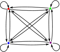
2pt $9$ [ ] at 32 1 $9$ [ ] at 34 197 $5$ [ ] at 200 199 $6$ [ ] at 202 9 $6$ [ ] at 15 106 $9$ [ ] at 48 106 $9$ [ ] at 118 187 $5$ [ ] at 118 154 $6$ [ ] at 185 106 $3$ [ ] at 217 106 $7$ [ ] at 118 18 $5$ [ ] at 117 50 $6$ [ ] at 142 140 $5$ [ ] at 160 117 $6$ [ ] at 76 117 $7$ [ ] at 95 140  2pt $12$ [ ] at 38 5 $13$ [ ] at 36 197 $11$ [ ] at 198 199 $12$ [ ] at 198 9 $8$ [ ] at 15 106 $12$ [ ] at 48 106 $13$ [ ] at 118 187 $8$ [ ] at 118 154 $12$ [ ] at 185 106 $8$ [ ] at 217 106 $13$ [ ] at 118 18 $10$ [ ] at 117 50 $10$ [ ] at 142 140 $9$ [ ] at 160 117 $9$ [ ] at 76 117 $10$ [ ] at 95 140

Figure 7.8. The graphs $W(\phi_{0,-1})$ (top left), $W(\phi_{1,-2})$ (top right), $W(\phi_{1,-3})$ (bottom left) and $W(\phi_{1,-4})$ (bottom right).

Case 2 ($k\geq 5$ is odd).

Note that $t^{\frac{k-1}{2}}u^{\frac{k+3}{2}}$ and $t^{-\frac{k+1}{2}}u^{\frac{k+1}{2}}$ are not in $\operatorname{Stash}(B,B)$, and both evaluate to $-\frac{(k+1)^{2}}{2}$ by $\phi_{1,-k}$. Hence $\frac{(k+1)^{2}}{2}\notin-\phi_{1,-k}(\operatorname{Stash}(B,B))$. One easily verifies that $\frac{(k+1)^{2}}{2}$ is in fact the largest integer that is not contained in $-\phi_{1,-k}(\operatorname{Stash}(B,B))$. Since $\operatorname{Stash}(B,R)=\operatorname{Stash}(B,B)$, it is also the largest integer not contained in $-\phi_{1,-k}(\operatorname{Stash}(B,R))$.

The set

$$Z_{k}=\left\{t^{a}u^{b}:-\frac{k-1}{2}\leq a\leq\frac{k-1}{2},b\geq\frac{k+3}{2}\right\}$$

is contained in $\operatorname{Stash}(R,R)$, $\operatorname{Stash}(R,B)$, $\operatorname{Stash}(R,G)$, $\operatorname{Stash}(R,P)$, $\operatorname{Stash}(B,G)$, $\operatorname{Stash}(G,G)$, $\operatorname{Stash}(G,R)$, $\operatorname{Stash}(G,B)$, $\operatorname{Stash}(P,G)$, $\operatorname{Stash}(P,B)$, $\operatorname{Stash}(P,R)$, so the weights of the corresponding edges are less than

$$k\frac{k+3}{2}-\frac{k-1}{2}=\frac{k^{2}+2k+1}{2}=\frac{(k+1)^{2}}{2}.$$

The set $tZ_{k}$ is contained in $\operatorname{Stash}(G,P)=\operatorname{Stash}(P,P)$, so the weights of the corresponding edges are strictly less than $\frac{(k+1)^{2}}{2}-1$. For the only remaining pair, $(B,P)$, one can check that $w(B,P)=\frac{(k+1)^{2}}{2}-1$.

Therefore $w(B,B)=w(B,R)=\frac{(k+1)^{2}}{2}$ and the weights of the other edges are strictly smaller. Therefore the largest average cycle weight is $\frac{(k+1)^{2}}{2}$, realized only by the loop on the blue vertex.

Case 3 ($k\geq 6$ is even).

The set

$$W_{k}=\left\{t^{a}u^{b}:-\frac{k}{2}\leq a\leq\frac{k-2}{2},b\geq\frac{k+2}{2}\right\}-\left\{t^{\frac{k-2}{2}}u^{\frac{k+2}{2}}\right\}$$

is contained in $\operatorname{Stash}(R,R)$, $\operatorname{Stash}(R,B)$, $\operatorname{Stash}(R,G)$, $\operatorname{Stash}(B,R)$, $\operatorname{Stash}(B,B)$, $\operatorname{Stash}(G,R)$, $\operatorname{Stash}(G,B)$, therefore the weights of the corresponding edges are at most

$$X_{k}=k\frac{k+2}{2}-\frac{k-2}{2}=\frac{k^{2}+k+2}{2}.$$

The set $tW_{k}$ is contained in $\operatorname{Stash}(R,P)$, $\operatorname{Stash}(B,G)$, $\operatorname{Stash}(G,G)$, $\operatorname{Stash}(P,G)$, $\operatorname{Stash}(P,B)$, $\operatorname{Stash}(P,R)$, therefore the weights of the corresponding edges are at most $X_{k}-1$.

The set $t^{2}W_{k}$ is contained in $\operatorname{Stash}(G,P)$, $\operatorname{Stash}(P,P)$, therefore the weights of the corresponding edges are at most $X_{k}-2$.

There is one remaining edge: $BP$. Using that neither $t^{-\frac{k-2}{2}}u^{\frac{k+2}{2}}$, nor $t^{\frac{k+2}{2}}u^{\frac{k+4}{2}}$ are in $\operatorname{Stash}(B,P)$ and both expressions evaluate to $\frac{k^{2}+3k-2}{2}$, one can verify that $w(B,P)=\frac{k^{2}+3k-2}{2}$. One can also check that $w(P,B)$ is in fact exactly $X_{k}-1$, therefore the cycle $BPB$ has average weight $\frac{k^{2}+2k-1}{2}$. Since this weight is larger than $X_{k}$, no other cycle can have the same of larger average weight.

∎

Finally, we give the proof of Theorem 1.6.

Proof of Theorem 1.6.

Parametrize the fibered face $\mathcal{F}$ with the interval $[-1,1]$, using the map $\phi_{a,b}\mapsto\frac{a}{b}$.

Using Lemma 7.5, we have $\|\phi_{0,-1}\|^{2}=4$ and $\|\phi_{\pm 1,-k}\|^{2}=4k^{2}$ for every integer $k\geq 2$. Together with Proposition 7.8, we obtain the values of $\mu_{1}(t)$ in Theorem 1.6 for $t\leq 0$. By the symmetry discussed in the proof of Lemma 7.5, we have $\mu_{1}(t)=\mu_{1}(-t)$ for all $t\in(-1,1)$, which yields the claimed values of $\mu_{1}(t)$ when $t>0$.

Using the substitution $t=\frac{a}{-\frac{1}{2}}$, hence $a=-\frac{1}{2}t$, in Proposition 7.7, we obtain that the set of accumulation points of the graph of $\mu_{1}(t)$ is the graph of

$$\frac{2}{(\frac{1}{2}+\frac{1}{2}t)(\frac{1}{2}-\frac{1}{2}t)}=\frac{8}{1-t^{2}}$$

as claimed. Finally, it is straightforward to check that $\mu_{1}(t)<\frac{8}{1-t^{2}}$ for all values of $t$ for which we have determined $\mu_{1}(t)$. ∎

References

- [Ago11] Ian Agol. Ideal triangulations of pseudo-Anosov mapping tori. In Topology and geometry in dimension three, volume 560 of Contemp. Math., pages 1–17. Amer. Math. Soc., Providence, RI, 2011.
- [BSW18] Hyungryul Baik, Hyunshik Shin, and Chenxi Wu. An upper bound on the asymptotic translation lengths on the curve graph and fibered faces. 01 2018.
- [FLP79] Albert Fathi, François Laudenbach, and Valentin Poénaru. Travaux de Thurston sur les surfaces, volume 66 of Astérisque. Société Mathématique de France, Paris, 1979. Séminaire Orsay, With an English summary.
- [FM12] Benson Farb and Dan Margalit. A primer on mapping class groups, volume 49 of Princeton Mathematical Series. Princeton University Press, Princeton, NJ, 2012.
- [Fri82a] David Fried. Flow equivalence, hyperbolic systems and a new zeta function for flows. Comment. Math. Helv., 57(2):237–259, 1982.
- [Fri82b] David Fried. The geometry of cross sections to flows. Topology, 21(4):353–371, 1982.
- [FS14] David Futer and Saul Schleimer. Cusp geometry of fibered 3-manifolds. Amer. J. Math., 136(2):309–356, 2014.
- [GT11] Vaibhav Gadre and Chia-Yen Tsai. Minimal pseudo-Anosov translation lengths on the complex of curves. Geom. Topol., 15(3):1297–1312, 2011.
- [Gué16] François Guéritaud. Veering triangulations and Cannon-Thurston maps. J. Topol., 9(3):957–983, 2016.
- [KS17] Eiko Kin and Hyunshik Shin. Small asymptotic translation lengths of pseudo-anosov maps on the curve complex. Groups, Geometry, and Dynamics, 07 2017.
- [McM00] Curtis T. McMullen. Polynomial invariants for fibered 3-manifolds and Teichmüller geodesics for foliations. Ann. Sci. École Norm. Sup. (4), 33(4):519–560, 2000.
- [MT17] Yair N. Minsky and Samuel J. Taylor. Fibered faces, veering triangulations, and the arc complex. Geom. Funct. Anal., 27(6):1450–1496, 2017.
- [Ota96] Jean-Pierre Otal. Le théorème d’hyperbolisation pour les variétés fibrées de dimension 3. Astérisque, (235):x+159, 1996.
- [RA05] J. L. Ramírez Alfonsín. The Diophantine Frobenius problem, volume 30 of Oxford Lecture Series in Mathematics and its Applications. Oxford University Press, Oxford, 2005.
- [Thu86] William P. Thurston. A norm for the homology of -manifolds. Mem. Amer. Math. Soc., 59(339):i–vi and 99–130, 1986.
- [Val14] Aaron D. Valdivia. Asymptotic translation length in the curve complex. New York J. Math., 20:989–999, 2014.