Bregman Divergence Bounds and
Universality Properties of the Logarithmic Loss

Abstract

A loss function measures the discrepancy between the true values and their estimated fits, for a given instance of data. In classification problems, a loss function is said to be proper if a minimizer of the expected loss is the true underlying probability. We show that for binary classification, the divergence associated with smooth, proper, and convex loss functions is upper bounded by the Kullback-Leibler (KL) divergence, to within a normalization constant. This implies that by minimizing the logarithmic loss associated with the KL divergence, we minimize an upper bound to any choice of loss from this set. As such the logarithmic loss is universal in the sense of providing performance guarantees with respect to a broad class of accuracy measures. Importantly, this notion of universality is not problem-specific, enabling its use in diverse applications, including predictive modeling, data clustering and sample complexity analysis. Generalizations to arbitary finite alphabets are also developed. The derived inequalities extend several well-known $f$-divergence results.

.

I Introduction

One of the major roles of statistical analysis is making predictions about future events and providing suitable accuracy guarantees. For example, consider a weather forecaster that estimates the chances of rain on the following day. Its performance may be evaluated by multiple statistical measures. We may count the number of times it assessed the chance of rain as greater than 50%, when there was eventually no rain (and vice versa). This corresponds to the so-called 0-1 loss, with threshold parameter $t=1/2$. Alternatively, we may consider a variety of values for $t$, or even a completely different measure. Indeed, there are many candidates, including the quadratic loss, Bernoulli log-likelihood loss, boosting loss, etc. [2]. Choosing a good measure is a well-studied problem, mostly in the context of scoring rules in decision theory [3, 4, 5, 6].

Assuming that the desired measure is known in advance, the predictor may be designed accordingly—i.e., to minimize that measure. However, in practice, different tasks may require inferring different information from the provided estimates. Moreover, designing a predictor with respect to one measure may result in poor performance when evaluated by another. For example, the minimizer of a 0-1 loss may result in an unbounded loss, when measured with a Bernoulli log-likelihood loss. In such cases, it would be desireable to design a predictor according to a “universal” measure, i.e., one that is suitable for a variety of purposes, and provide performance guarantees for different uses.

In this paper, we show that for binary classification, the Bernoulli log-likelihood loss (log-loss) is such a universal choice, dominating all alternative “analytically convenient” (i.e., smooth, proper, and convex) loss functions. Specifically, we show that by minimizing the log-loss we minimize the regret associated with all possible alternatives from this set. Our result justifies the use of log-loss in many applications.

As we develop, our universality result may be equivalently viewed from a divergence analysis viewpoint. In particular, we establish that the divergence associated with the log-loss—i.e., Kullback Leibler (KL) divergence—upper bounds a set of Bregman divergences that satisfy a condition on its Hessian. Additionally, we show that any separable Bregman divergence that is convex in its second argument is a member of this set. This result provides a new set of Bregman divergence inequalities. In this sense, our Bregman analysis is complementary to the well-known $f$-divergence inequality results [7, 8, 9, 10].

We further develop several applications for our results, including universal forecasting, universal data clustering, and universal sample complexity analysis for learning problems, in addition to establishing the universality of the information bottleneck principle. We emphasize that our universality results are derived in a rather general setting, and not restricted to a specific problem. As such, they may find a wide range of additional applications.

The remainder of the paper is organized as follows. Section II summarizes related work on loss function analysis, universality and divergence inequalities. Section III provides the needed notation, terminology, and definitions. Section IV contains the main results for binary alphabets, and their generalization to arbitrary finite alphabets is developed in Section V. Additional numerical analysis and experimental validation is provided in Section VI, and the implications of our results in three distinct applications is described in Section VII. Finally, Section VIII contains some concluding remarks.

II Related Work

The Bernoulli log-likelihood loss function plays a fundamental role in information theory, machine learning, statistics and many other disciplines. Its unique properties and broad applications have been extensively studied over the years.

The Bernoulli log-likelihood loss function arises naturally in the context of parameter estimation. Consider a set of independent, identically distributed (i.i.d.) observations $y^{n}=(y_{1},\dots,y_{n})$ drawn from a distribution $p_{Y}(\cdot;\theta)$ whose parameter $\theta$ is unknown. Then the maximum likelihood estimate of $\theta$ in  -$\mathcal{O}$ is

$$\hat{\theta}=\operatorname*{arg\,max}_{\theta\in\text{$\hbox to0.0pt{\hbox to5.44446pt{\hss\raisebox{0.60275pt}{\hskip 0.49005pt{-}}\hss}\hss}\hbox{$\mathcal{O}$}$}}L(\theta;y^{n}),$$

where

$$L(\theta;y^{n})=p_{Y^{n}}(y^{n};\theta)=\prod_{i=1}^{n}p_{Y}(y_{i};\theta).$$

Intuitively, it selects the parameters values that make the data most probable. Equivalently, this estimate minimizes a loss that is the (negative, normalized, natural) logarithm of the likelihood function, viz.,

$$\ell(\theta;y^{n})\triangleq-\frac{1}{n}\log L(\theta;y^{n})=-\frac{1}{n}\sum_{i=1}^{n}\log p_{Y}(y_{i};\theta),$$

whose mean is

$${\mathbb{E}}\left[\ell(\theta;Y)\right]=-{\mathbb{E}}\left[\log p_{Y}(Y;\theta)\right].$$

Hence, by minimizing this Bernoulli log-likelihood loss, termed the log-loss, over a set of parameters we maximize the likelihood of the given observations.

The log-loss also arises naturally in information theory. The self-information loss function $-\log p_{Y}(y)$ defines the ideal codeword length for describing the realization $Y=y$ [11]. In this sense, minimizing the log-loss corresponds to minimizing the amount of information that are necessary to convey the observed realizations. Further, the expected self-information is simply Shannon’s entropy which reflects the average uncertainty associated with sampling the random variable $Y$.

The logarithmic loss function is known to be “universal” from several information-theoretic points of view. In [12], Feder and Merhav consider the problem of universal sequential prediction, where a future observation is to be estimated from a given set of past observations. The notion of universality comes from the assumption that the underlaying distribution is unknown, or even nonexistent. In this case, it is shown that if there exists a universal predictor (with a uniformly rapidly decaying redundancy rates) that minimizes the logarithmic loss function, then there exist universal predictors for any other loss function.

More recently, No and Weissman [13] introduced log-loss universality results in the context of lossy compression. They show that for any fixed length lossy compression problem under an arbitrary distortion criterion, there is an equivalent lossy compression problem under a log-loss criterion where the optimum schemes coincide. This result implies that without loss of generality, one may restrict attention to the log-loss problem (under an appropriate reconstruction alphabet). In addition, [13] considers the successive refinement problem, showing that if the first decoder operates under log-loss, then any discrete memoryless source is successively refinable under an arbitrary distortion criterion for the second decoder.

It is important to emphasize that universality results of the type discussed above are largely limited to relatively narrowly-defined problems and specific optimization criteria. By contrast, our development is aimed at a broader notion of universality that is not restricted to a specific problem, and considers a broader range of criteria.

An additional information-theoretic justification for the wide use of the log-loss is introduced in [14]. This work focuses on statistical inference with side information, showing that for an alphabet size greater than two, the log-loss is the only loss function that benefits from side information and satisfies the data processing lemma. This result extends some well-known properties of the log-loss with respect to the data processing lemma, as later described.

Within decision theory, statistical learning and inference problems, the log-loss also plays further key role in the context of proper loss function, which produce estimates that are unbiased with respect to the true underlaying distribution. Proper loss functions have been extensively studied, compared, and suggested for a variety of tasks [3, 4, 15, 5, 6]. Among these, the log-loss is special: it is the only proper loss that is local [16, 17]. This means that the log-loss is the only proper loss function that assigns an estimate for the probability of the event $Y=y_{0}$ that depends only on the outcome $Y=y_{0}$.

In turn, proper loss functions are closely related to Bregman divergences, with which there exists a one-to-one correspondence [4]. For the log-loss, the associated Bregman divergence is KL divergence, which is also an instance of an $f$-divergence [18]. Significantly, for probability distributions, the KL divergence is the only divergence measure that is a member of both of these classes of divergences [19]. The Bregman divergences are the only divergences that satisfy a “mean-as-minimizer” property [20], while any divergence that satisfy the data processing inequality is necessarily an $f$-divergence (or a unique (one-to-one) mapping thereof) [21]. As a consequence, any divergence that satisfies both of these important properties simultaneously is necessarily proportional to the KL divergence [22, Corollary 6]. Additional properties of KL divergence are also discussed in [22].

Finally, divergences inequalities have been studied extensively. The most celebrated example is the Pinsker inequality [23], which expresses that KL divergence upper bounds the squared total-variation distance. More recently, the detailed studies of Reid and Williamson [10], Harremoës and Vajda [9], Sason and Verdú [8], and Sason [7] have extended this result to a broader set of $f$-divergences inequalities. Moreover, $f$-divergence inequalities for non-probability measures appear in, e.g., by Stummer and Vajda [24]. In [25], Zhang demonstrated an important Bregman inequality in the context of statistical learning, showing that the KL divergence upper bounds the squared excess-risk associated with the 0-1 loss, and thus controls this traditionally important performance measure. Within this context, our work can be viewed as extending such Bregman inequalities and their analysis.

III Notation, Terminology and Definitions

Let $Y\in\{0,1\}$ be a Bernoulli random variable with parameter $p=p_{Y}(1)$, which may be unknown. A loss function $l(y,\hat{y})$ quantifies the discrepancy between a realization $Y=y$ and its corresponding estimate $\hat{y}$. In this work we focus on probabilistic estimates $\hat{y}\triangleq q\in[0,1]$ whereby $q$ is an estimate of $p$ rather than $y$ itself; as such, $q$ is a “soft” decision.

A loss function for such estimation takes the form

$$l(y,q)=\mathbbb{1}\{y=0\}\,l_{0}(q)+\mathbbb{1}\{y=1\}\,l_{1}(q),$$ (1)

with $\mathbbb{1}\{\cdot\}$ denoting the Kronecker (indicator) function, where $l_{k}(q)$ is a loss function associated with the event $Y=k$, for $k\in\{0,1\}$. In turn, the corresponding expected loss is

$$L(p,q)\triangleq{\mathbb{E}}\left[l(Y,q)\right]=(1-p)\,l_{0}(q)+p\,l_{1}(q),$$ (2)

where we note that $L(p,q)$ depends only on $p$ and the estimate $q$. An example is the log-loss, for which

$$l_{\log}(y,q)\triangleq y\log\frac{1}{q}+(1-y)\log\frac{1}{1-q}.$$ (3)

Loss functions with additional properties are of particular interest. A loss function is proper (or, equivalently, Fisher-consistent or unbiased) if a minimizer of the expected loss is the true underlying distribution of the random variable we are to estimate; specifically,

$$p\in\operatorname*{arg\,min}_{q\in[0,1]}{L(p,q)},\quad p\in[0,1].$$ (4)

A strictly proper loss function means that $q=p$ is the unique minimizer, i.e.,

$$p=\operatorname*{arg\,min}_{q\in[0,1]}{L(p,q)},\quad p\in[0,1].$$ (5)

A proper loss function is fair if

$$l_{0}(0)=l_{1}(1)=0,$$ (6)

in which case there is no loss incurred for accurate prediction. Additionally, a proper loss function is regular if

$$\lim_{q\to 0}q\,l_{1}(q)=\lim_{q\to 1}(1-q)\,l_{0}(q)=0.$$ (7)

Intuitively, (7) ensures that making mistakes on events that cannot happen do not incur a penalty.

The minimum of the expected loss for proper loss functions, which we denote using

$$G(p)\triangleq L(p,p),$$

is referred to as the generalized entropy function [4], Bayes risk [26] or Bayesian envelope [27]. As an example, the Shannon entropy associated with the log-loss (3) is

$$G_{\log}(p)\triangleq p\log\frac{1}{p}+(1-p)\log\frac{1}{1-p}.$$ (8)

The regret is defined as the difference between the expected loss and its minimum, so for proper loss functions takes the form

$$\Delta L(p,q)=L(p,q)-G(p).$$ (9)

Savage [28] shows that a loss function $l(y,q)$ is proper and regular if and only if $G(\cdot)$ is concave and for every $p,q\in[0,1]$ we have that

$$L(p,q)=G(q)+(p-q)\,G^{\prime}(q).$$ (10)

This property allows us to draw an immediate connection between regret and Bregman divergence. In particular, let $f\colon\mathcal{S}\mapsto\mathbb{R}$ be a continuously differentiable, strictly convex function over some interval $\mathcal{S}\subset\mathbb{R}$. Then its associated Bregman divergence takes the form

$$D_{f}(s\|t)\triangleq f(s)-f(t)-(s-t)f^{\prime}(t)$$ (11)

for any $s,t\in\mathcal{S}$. We focus on closed intervals, in which case the formal definition of $D_{f}(s\|t)$ at boundary points requires more care; the details are summarized in Appendix A, following [29].

In the special case $\mathcal{S}=[0,1]$ using (10) in (9) and comparing the result to (11) we obtain

$$\Delta L(p,q)=D_{-G}(p,q),$$ (12)

i.e., the regret of a proper loss function is uniquely associated with a Bregman divergence. As an important example, associated with the Shannon entropy (8) is the KL divergence

$$D_{\mathrm{KL}}(p\|q)\triangleq p\log\frac{p}{q}+(1-p)\log\frac{1-p}{1-q}.$$ (13)

Of particular interest are loss functions that are convex, i.e., $l$ such that $l(y,\cdot)$ is convex. Such loss functions play a special role in learning theory and optimization [2, 26]. For example, suppose $X^{d}$ and $Y$ is a set of $d$ explanatory variables (features) and a (target) variable, respectively. Then given a set of $n$ i.i.d. samples of $X^{d}$ and $Y$, the empirical risk minimization (ERM) criterion seeks to minimize

$$\frac{1}{n}\sum_{i=1}^{n}l(y_{i},q_{i}),$$

where $q_{i}\triangleq q_{i}(x^{d}_{i})$ denotes a functional of the $i$th sample of $X^{d}$. This minimization is much easier to carry out when the loss function $l$ is convex, particularly when $d$ is large. In addition, the minimum of the expected loss $L(p,\cdot)$ for a given $p$ subject to constraints is typically much easier to characterize and compute when $l$ is convex.

Conveniently, convex proper loss functions $l(y,q)$ correspond to Bregman divergences $D_{-G}$ such that $D_{-G}(p\|\cdot)$ is convex [26]. This family of divergences are of special interest in many applications [30, 31], and have an important role in our results, as will become apparent.

Accordingly, our development emphasizes the following class of analytically convenient loss functions.

Definition 1

A loss function $l\colon\{0,1\}\times[0,1]\mapsto\mathbb{R}$, which takes the form (1), is admissible if it satisfies the following three properties:

1. $l(y,q)$ is strictly proper, fair, and regular, i.e., satisfies (5)–(7).

2. $l(y,\cdot)$ is convex for each $y\in\{0,1\}$.

3. $l(y,\cdot)$ is in $\mathcal{C}^{3}$ for each $y\in\{0,1\}$, i.e., ${\partial^{k}l(y,q)}/{\partial q^{k}}$ exist and are continuous for $k=1,2,3$.

For convenience, we refer to loss functions that satisfy property P1.3 as smooth.

As further terminology, for a proper, smooth loss function $l(y,q)$ with generalized entropy $G(p)$,

$$w(p)\triangleq-G^{\prime\prime}(p)$$ (14)

is referred to as its weight function, which we note is nonnegative. As an example, that corresponding to the log-loss is

$$w_{\mathrm{KL}}(q)=\frac{1}{q(1-q)}.$$ (15)

Using (14), we obtain, for example,

$$\frac{\partial}{\partial q}D_{-G}(p\|q)=(q-p)\,w(q),$$ (16)

by differentiating (10), which emphasizes the one-to-one correspondence between $D_{-G}$ and $w$ for such loss functions; see Appendix B for additional properties and characterizations.

Finally, representative examples of loss functions are provided in Table I, along with their generalized entropies, their associated Bregman divergences, and their weight functions.

Table I: Examples of Commonly Used Binary Loss Functions

[1]0 Loss function	$l(y,q)$	$G(p)=L(p,p)$	$D_{-G}(p\|q)$	$w(p)$
[1]0 Quadratic loss	$y(1-q)^{2}+(1-y)q^{2}$	$p(1-p)$	$D_{\mathrm{QL}}(p\|q)=(p-q)^{2}$	$2$
[1]0 Logarithmic loss	$\begin{aligned} y&\log\textstyle\frac{1}{q}\\ &{}+(1\!-\!y)\log\textstyle\frac{1}{1-q}\\ \ \end{aligned}$	$\begin{aligned} p&\log\textstyle\frac{1}{p}\\ &{}+(1-p)\log\textstyle\frac{1}{1-p}\\ \end{aligned}$	$D_{\mathrm{KL}}(p\|q)=p\log\frac{p}{q}+(1-p)\log\frac{1-p}{1-q}$	$\frac{1}{p(1-p)}$
[1]0 Boosting loss	$\begin{aligned} 2y&\textstyle\sqrt{\frac{1-q}{q}}\\ &{}+2(1-y)\textstyle\sqrt{\frac{q}{1-q}}\\ \ \end{aligned}$	$4\sqrt{p(1-p)}$	$\begin{aligned} D_{\mathrm{BL}}(p\|q)=2\biggl{(}p\textstyle\sqrt{\frac{1-q}{q}}+(1\!&-\!p)\textstyle\sqrt{\frac{q}{1-q}}\biggr{)}\\ &{}-4\textstyle\sqrt{p(1-p)}\end{aligned}$	$\frac{1}{(p(1-p))^{3/2}}$

IV Universality Properties of the Logarithmic Loss Function

Our main result is as follows, a proof of which is provided in Appendix C.

Theorem 1

Given a loss function $l(y,q)$ satisfying Definition 1 with corresponding generalized entropy function $G$, then for every $p,q\in[0,1]$,

$$D_{\mathrm{KL}}(p\|q)\geq\frac{1}{C(G)}D_{-G}(p\|q),$$ (17a)

where

$$C(G)>-\frac{1}{2}\,G^{\prime\prime}\biggl{(}\frac{1}{2}\biggr{)}$$ (17b)

is a positive normalization constant (that does not depend on $p$ or $q$).

Note that a further consequence of Theorem 1 expresses that KL divergence is a “dominating” Bregman divergence in the sense that given another Bregman divergence $\tilde{D}(p\|q)$ such that [cf. (17a)]

$$\tilde{D}(p\|q)\geq\frac{1}{\tilde{C}(G)}D_{-G}(p\|q)$$

holds for any Bregman divergence $D_{-G}$ for some $\tilde{C}(G)$, then the theorem asserts that there exists $\tilde{C}_{\mathrm{KL}}$ such that

$$D_{\mathrm{KL}}(p\|q)\geq\frac{1}{\tilde{C}_{\mathrm{KL}}}\,\tilde{D}(p\|q).$$

In essence, the dominating Bregman divergences form an equivalence class, of which KL divergence is a member.

We emphasize the necessity of scaling constants in Theorem 1. Indeed, the class of loss functions satisfying Definition 1 is closed under (nonnegative) scaling, i.e., if $l(y,q)$ (with a corresponding $G$) satisfies Definition 1, then so does $\gamma l(y,q)$—with a corresponding $\gamma G$—for any $\gamma>0$. A typical approach to placing loss functions on a common scale is to define a universal scaling by setting, for instance,

$$-\frac{1}{2}\,G^{\prime\prime}\biggl{(}\frac{1}{2}\biggr{)}=1,$$

as appears, e.g., in [2, 10]. Theorem 1 avoids imposing such a normalization, and instead absorbs such scaling into the constant $C(G)$ to obtain the desired invariance. As an example, for the quadratic loss $G^{\prime\prime}(1/2)=-2$, so any $C(G)>1$ suffices in this case, whence

$$D_{\mathrm{KL}}(p\|q)\geq(p-q)^{2}.$$ (18)

The practical implications of Theorem 1 are quite immediate. Assume that the performance measure according to which a learning algorithm is to be measured is unknown a priori to the application (as is the case, e.g., in the weather forecasting example of Section I). In such cases, minimizing the log-loss provides an upper bound on any possible choice of measure that is associated with an “analytically convenient” loss function. As such, the log-loss is a universal choice for classification problems with respect to this class of measures.

More generally, as discussed in Section II, designing suitable loss functions is an active research field with many applications. Via Theorem 1, one obtains universality guarantees for any (current or future) loss function that is proper, convex, and smooth. We emphasize that this class of loss functions is quite rich. For instance, it is straightforward to verify that the loss functions satisfying Definition 1 form a convex set: any convex combination of such loss functions also satisfies Definition 1.

The local behavior of proper, convex, and smooth loss functions can be derived from Theorem 1. In particular, we have the following corollary.

Corollary 2

Given a loss function $l(y,q)$ satisfying Definition 1, whose corresponding generalized entropy function is $G$, we have, for every $p,p+\mathrm{d}p\in[0,1]$ and some finite $C(G)>0$,

$$\frac{1}{C(G)}\,D_{-G}(p\|p+\mathrm{d}p)\leq\frac{\mathrm{d}p^{2}}{2}\,J(p)+o(\mathrm{d}p^{2}),$$ (19a)

where

$$J(p)\triangleq\frac{1}{p(1-p)}$$ (19b)

denotes the Fisher information of a Bernoulli distributed random variable with parameter $p$.

Proof:

With $p,p+\mathrm{d}p\in[0,1]$, the Taylor series expansion of the KL divergence around $p$ is

$$D_{\mathrm{KL}}(p\|p+\mathrm{d}p)=\frac{\mathrm{d}p^{2}}{2}J(p)+o(\mathrm{d}p^{2}),$$ (20)

where $J(p)$ is as given in (19b). Substituting (20) into (17a) yields the desired inequality. ∎

Corollary 2 establishes that when $q$ is sufficiently close to $p$, the divergence associated with the set of smooth, proper and convex binary loss functions is effectively upper bounded by the Fisher information that locally characterizes KL divergence. As such, we conclude that the rate of convergence of any $D_{-G}(p\|q)$ to zero as $q\to p$ is upper bounded by the rate of $D_{\mathrm{KL}}(p\|q)$. This reveals that the price paid for the universality of the log-loss is its slower rate of convergence. Such behavior will be demonstrated empirically in Section VI.

V Extended Bregman Divergence Inequalities

To extend our result to arbitrary finite alphabets, we consider the corresponding broader class of Bregman divergences. In particular, for a continuously differentiable, strictly convex function $f\colon\mathcal{S}\mapsto\mathbb{R}$ be a over some convex set $\mathcal{S}\subset\mathbb{R}^{m}$, its associated Bregman divergence takes the form

$$D_{f}(s^{m}\|t^{m})\triangleq f(s^{m})-f(t^{m})-\langle s^{m}-t^{m},\nabla f(t^{m})\rangle$$ (21)

for any $s^{m},t^{m}\in\mathcal{S}$ when $\mathcal{S}$ is open, where $\nabla f(t^{m})$ is the gradient of $f$ at $t^{m}$.

We focus on the set $\mathcal{S}=[0,1]^{m}$, and let $p^{m},q^{m}\in\mathcal{S}$. We emphasize that this is an extension beyond the unit simplex. Let

$$H_{f}(p^{m})\triangleq\nabla^{2}f(p^{m})$$ (22)

denote the $m\times m$ Hessian matrix of $f$. For example, the divergence associated with

$$f(p^{m})=\sum_{i=1}^{m}p_{i}\log p_{i}$$ (23)

is the generalized $\mathrm{KL}$ divergence

$$\tilde{D}_{\mathrm{KL}}(p^{m}\|q^{m})\triangleq\sum_{i=1}^{m}p_{i}\log\frac{p_{i}}{q_{i}}-\sum_{i=1}^{m}p_{i}+\sum_{i=1}^{m}q_{i},$$ (24)

the corresponding Hessian for which is

$$H_{\mathrm{KL}}(p^{m})\triangleq\nabla^{2}\left(\sum_{i=1}^{m}p_{i}\log p_{i}\right),$$

which we note is a diagonal matrix whose $i$th diagonal element is $1/p_{i}$. In the special case wherein $p^{m}$ and $q^{m}$ are probability measures (i.e., restricted to the unit simplex), we have

$$\tilde{D}_{\mathrm{KL}}(p^{m}\|q^{m})=D_{\mathrm{KL}}(p^{m}\|q^{m})\triangleq\sum_{i=1}^{m}p_{i}\log\frac{p_{i}}{q_{i}},$$

which generalizes the definition in Table I.

We focus on the following class of Bregman divergences.

Definition 2

For some integer $K$, a Bregman divergence generator $f\colon[0,1]^{m}\mapsto\mathbb{R}$ is $K$-admissible if it satisfies the following properties:

1. $f$ is a strictly convex function that is well-defined on its boundaries, in the sense of generalizing the requirements of Appendix A.

2. $f\in\mathcal{C}^{K}$, i.e., ${\partial^{k}f(p^{m})}/{\partial p_{1}\cdots\partial p_{k}}$ exist and are continuous for $k=1,\dots,K$.

Our first generalization is the following theorem, whose proof is provided in Appendix D.

Theorem 3

Given a positive integer $m$, let $f\colon[0,1]^{m}\mapsto\mathbb{R}$ satisfy Definition 2 for $K=2$, and let $D_{f}(p^{m}\|q^{m})$ and $H_{f}(p^{m})$ denote the associated Bregman divergence and Hessian matrix, respectively. If there exists a (finite) positive constant $C(f)$ such that

$$C(f)\,H_{\mathrm{KL}}(p^{m})-H_{f}(p^{m})\succ 0,\quad\text{all $p^{m}\in[0,1]^{m}$},$$ (25a)

then for every $$p^{m},q^{m}\in[0,1]^{m}$$,

$$\tilde{D}_{\mathrm{KL}}(p^{m}\|q^{m})\geq\frac{1}{C(f)}\,D_{f}(p^{m}\|q^{m}).$$ (25b)

We emphasize that, in contrast to Theorem 1, the inequality (25b) applies to any Bregman divergence satisfying Definition 2, and in particular does not require $D_{f}(p^{m}\|\cdot)$ to be convex for any $p^{m}\in[0,1]^{m}$. However, at the same time, we stress that Theorem 3 is restricted to the class of divergences satisfying (25a).

As an example application, when

$$f(p^{m})=(p^{m})^{\mathrm{T}}Q\,p^{m},$$ (26)

with positive definite matrix parameter $Q$, the corresponding the Bregman divergence

$$D_{f}=\frac{1}{2}(p^{m}-q^{m})^{\mathrm{T}}Q\,(p^{m}-q^{m})$$

is the well-known Mahalanobis distance, and and the associated Hessian is

$$H_{f}(p^{m})=Q.$$

For this divergence we have the following corollary, whose proof is provided in Appendix E.

Corollary 4

If $D_{f}$ is a Mahalanobis distance, whereby $f$ takes the form (26) with $Q\succ 0$, then (25b) holds for

$$C(Q)>\lambda_{\max}(Q),$$ (27)

where $\lambda_{\max}(Q)$ is the largest eigenvalue of $Q$.

Our second generalization of Theorem 1 focuses on the class of separable Bregman divergences, a member of which takes the form

$$D_{g}(p^{m}\|q^{m})\triangleq\sum_{i=1}^{m}d_{g}(p_{i}\|q_{i})$$ (28a)

with

$$d_{g}(p_{i}\|q_{i})\triangleq g(p_{i})-g(q_{i})-(p_{i}-q_{i})\,g^{\prime}(q_{i}),$$ (28b)

for $p^{m},q^{m}\in(0,1)^{m}$, where $g\colon[0,1]\mapsto\mathbb{R}$ denote a continuously differentiable, strictly convex function with additional constraints discussed analogous to those discussed in Appendix A, and via which (28a) is extended to $p^{m},q^{m}\in[0,1]^{m}$.

Such divergences hold a special role in divergence analysis, as discussed in, e.g., [22, 32]. Note that in this case, the Bregman generator function takes the form

$$f_{\mathrm{KL}}(p^{m})=\sum_{i=1}^{m}g(p_{i}),$$ (29)

via which we obtain the Hessian as

$$H_{f}(p^{m})=\mathbbb{1}\{i=j\}\,g^{\prime\prime}(p_{i}).$$

As an example,

$$g(p)=p\log p$$ (30)

matches (23), and when used in (28b) yields

$$\tilde{d}_{\mathrm{KL}}(p_{i}\|q_{i})\triangleq p_{i}\log\frac{p_{i}}{q_{i}}-p_{i}+q_{i},$$ (31)

so that (28a) specializes to the generalized KL divergence (24).

Our main result is the following theorem, a proof of which is provided in Appendix F.

Theorem 5

Given a positive integer $m$, let $D_{g}(p^{m}\|q^{m})$ be a separable Bregman divergence satisfying Definition 2 for $K=3$ and for which $D_{g}(p^{m}\|\cdot)$ is convex for every $p^{m}\in[0,1]^{m}$. Then for every $p^{m},q^{m}\in[0,1]^{m}$,

$$\tilde{D}_{\mathrm{KL}}(p^{m}\|q^{m})\geq\frac{1}{C(g)}D_{g}(p^{m}\|q^{m})$$ (32a)

when $$C(G)$$ satisfies

$$C(g)>g^{\prime\prime}(1).$$ (32b)

We remark that when $g^{\prime\prime}(1)$ is unbounded, Corollary 5 does not yield a useful bound. By contrast, Theorem 1 is guaranteed to produce a bound, since $G^{\prime\prime}(1/2)$ is always finite.

It is important to emphasize that while Theorem 1 restricts attention to divergences defined both over binary alphabets and only on the unit simplex—i.e., in the notation of this section,

$$m=2,\qquad p_{1}=p,\qquad p_{2}=1-p,\qquad p\in[0,1],$$

by contrast the divergences in Theorem 5 are defined for any positive integer $m$ and, in addition, over the entire hypercube $p^{m},q^{m}\in[0,1]^{m}$. As such, we emphasize that Theorem 1 is not a special case of Theorem 5. In particular, because (17a) must hold for a domain that extends beyond the unit simplex, the smallest $C(g)$ for which it is satisfied when $m=2$ must generally be bigger than the smallest $C(G)$ for which (17a) holds.

As a simple application of Theorem 5, choosing $g(p)=p^{2}$ generates the quadratic divergence

$$D_{g}(p\|q)=\sum_{i=1}^{m}(p_{i}-q_{i})^{2},$$

which is a special case of the Mahalanobis distance. In this case, since $g^{\prime\prime}(1)=2$, Theorem 5 requires $C(g)>2$, yielding

$$\tilde{D}_{\mathrm{KL}}(p^{m}\|q^{m})\geq\frac{1}{2}\sum_{i=1}^{m}(p_{i}-q_{i})^{2}.$$ (33)

Consistent with the preceding discussion, $\inf\{C(g)\colon C(g)>2\}=2$ corresponding to (33), is larger than the corresponding $\inf\{C(G)\colon C(G)>1\}=1$ in the bound (18).

Additionally, it is worth noting that (33) resembles the well-known Pinsker inequality [11], viz.,

$$D_{\mathrm{KL}}(p^{m}\|q^{m})\geq\frac{1}{2}D^{2}_{\mathrm{TV}}(p^{m}\|q^{m}),$$ (34)

where

$$D_{\mathrm{TV}}(p^{m}\|q^{m})\triangleq\sum_{i=1}^{m}|p_{i}-q_{i}|$$ (35)

is the total-variation distance (or Csiszár divergence [11]), which is not a Bregman divergence, but rather an $f$-divergence. It is straightforward to verify that (34) is tighter than (33) when $p^{m}$ and $q^{m}$ are restricted to the unit simplex. Nevertheless, this simple example serves to illustrate that Theorem 3 and Theorem 5 may be viewed as Bregman divergences extensions to some well-known $f$-divergence results, as discussed in Section II.

VI Numerical Analysis and Experiments

To complement the results of Section V, we use numerical analysis to examine the dependence of

$$\tilde{D}_{\mathrm{KL}}(p^{m}\|q^{m})-\frac{1}{C(f)}D_{f}(p^{m}\|q^{m})$$

on $p^{m}$ and $q^{m}$, for some choices of $f$ such that Theorem 3 applies, and with $C(f)$ chosen according to (25a).

To begin, we consider a random variable $Y\in\mathcal{Y}$ with $|\mathcal{Y}|=m$, and restrict $q^{m}$ to lie in a subset $\mathcal{S}$ of the unit simplex $\mathcal{P}^{\mathcal{Y}}$. For a given $p^{m}\in\mathcal{P}^{\mathcal{Y}}$, with

$$q^{m}_{f}(\mathcal{S})\triangleq\operatorname*{arg\,min}_{\{q^{m}\in\mathcal{S}\subset\mathcal{P}^{\mathcal{Y}}\}}D_{f}(p^{m}\|q^{m})$$ (36)

and, in turn,

$$q^{m}_{\mathrm{KL}}(\mathcal{S})\triangleq q^{m}_{f_{\mathrm{KL}}}(\mathcal{S}),$$ (37)

where $f_{\mathrm{KL}}$ is as given in (29), the minimum KL divergence upper bounds the minimum of any Bregman divergence according to

$$D_{\mathrm{KL}}(p^{m}\|q_{\mathrm{KL}}^{m}(\mathcal{S})) \geq\frac{1}{C(f)}D_{f}(p^{m}\|q_{\mathrm{KL}}^{m}(\mathcal{S}))$$

$$\qquad\qquad{}\geq\frac{1}{C(f)}D_{f}(p^{m}\|q_{f}^{m}(\mathcal{S})),$$ (38)

where to obtain the first inequality we have used Theorem 3 with $C(f)$ satisfying (25a), and to obtain the second inequality we have used (36).

In the first experiment, we set

$$\mathcal{S}=\bigl{\{}q^{m}\in\mathcal{P}^{\mathcal{Y}}\colon{\mathbb{E}}_{q^{m}}\left[h(Y)\right]=\mu\bigr{\}},$$

for some $h\colon\mathcal{Y}\mapsto\mathbb{R}$ and $\mu$, i.e., we constrain $q^{m}$ to lie in a hyperplane restricted to the unit simplex $\mathcal{P}^{\mathcal{Y}}$. More specifically, we choose $\mathcal{Y}=\{-1,0,1\}$, $h(y)=y$, and $p^{3}=(1/4,1/2,1/4)$ to illustrate our results. The results of our experiment, which compares the minima in (38) as a function of $\mu$, are depicted in Fig. 1. The top (blue) curve is (with a minor abuse of notation) $D_{\mathrm{KL}}(p^{3}\|q^{3}_{\mathrm{KL}}(\mu))$, and the progressively lower (red, purple, and black) curves are (with a similar abuse of notation) $D_{f}(p^{3}\|q^{3}_{f}(\mu))/C(f)$ with $f$ corresponding to the quadratic divergence, the separable Mahalanobis distance with parameters $Q_{\mathrm{s}}$, and the nonseparable Mahalanobis distance with parameters $Q_{\mathrm{ns}}$, respectively. The specific values of these parameters are

$$Q_{\mathrm{s}}=\begin{bmatrix}3&0&0\\ 0&2&0\\ 0&0&1\end{bmatrix}\quad\text{and}\quad Q_{\mathrm{ns}}=\begin{bmatrix}3&1/2&1/2\\ 1/2&2&1/2\\ 1/2&1/2&1\end{bmatrix}.$$ (39)

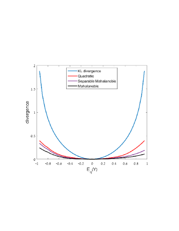
Figure 1: Divergence bound behavior under mean constraint. Depicted is the minimum of $D_{f}(p^{3}\|q^{3})/C(f)$ with respect to $q^{3}\in\mathcal{P}^{\mathcal{Y}}$ with ${\mathbb{E}}_{q^{3}}\left[Y\right]$ fixed, for $Y\in\mathcal{Y}=\{-1,0,1\}$, $p^{3}=\left(1/4,1/2,1/4\right)$, and different choices for $f$, as described in text.

Note that since ${\mathbb{E}}_{p^{3}}\left[Y\right]=0$ for our choice of $p^{3}$, all the minimum divergences are zero at $\mu={\mathbb{E}}_{q^{3}}\left[Y\right]=0$, and thus $\smash{q^{3}_{f}(0)=p^{3}}$ for all Bregman generators $f$. However, when $\mu\neq 0$, the optimizing $q^{3}_{f}(\mu)$ must differ from $p^{3}$, and Fig. 1 quantifies these differences as a function of the bias $\mu$. Consistent with the analysis of Section V, KL divergence upper bounds normalized measures of all these differences.

In the second experiment we show that the bounds (38) hold for a broader range of problems. To model a statistical, computational, or even algorithmic constraint that prevents $q^{m}$ from converging to some given $p^{m}\in\mathcal{P}^{\mathcal{Y}}$, we impose that $q^{m}\in\mathcal{S}$ where

$$\mathcal{S}=\{q^{m}\in\mathcal{P}^{\mathcal{Y}}\colon D(p^{m}\|q^{m})\geq\epsilon\}$$ (40)

for some $D$ and $\epsilon>0$. In Fig. 2, we compare the terms in (38) for different choices for $f$, and two different (non-Bregman) examples of $D$ in (40). In particular, the upper plots corresponds to choosing for $D$ in (40) the total-variation distance $D_{\mathrm{TV}}$ as defined in (35). For constrast, the lower plots corresponds choosing for $D$ in (40) the (Neyman) chi-square divergence, i.e.,

$$D_{\chi^{2}}(p^{m}\|q^{m})=\sum_{i=1}^{m}\frac{(p_{i}-q_{i})^{2}}{q_{i}}.$$ (41)

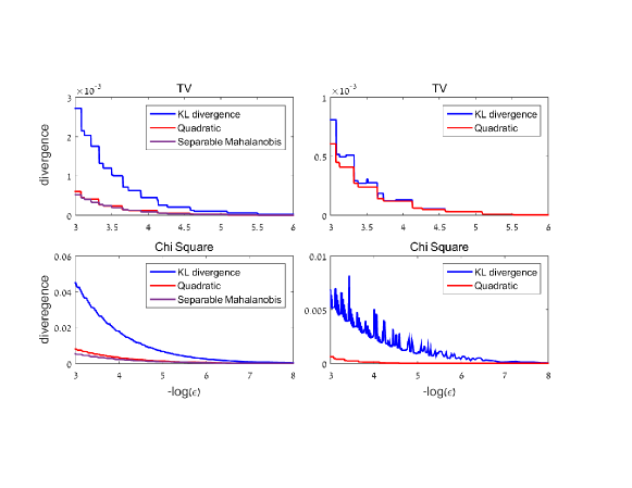
Figure 2: Divergence bound behavior under a divergence constraint. On the left is depicted the minimum of $D_{f}(p^{3}\|q^{3})/C(f)$ over $q^{3}$ for $p^{3}=(1/4,1/2,1/4)$ subject to $\smash{D(p^{3}\|q^{3})\geq\epsilon}$. In the plots on the right, the minimizing $\smash{q^{3}}$ is replaced with that minimizing KL divergence. The upper and lower plots correspond to $D$ being total-variation and chi-square divergences, respectively. The different choices for $f$ are as in Fig. 1.

The plots on the left compare $D_{\mathrm{KL}}(p^{m}\|q_{\mathrm{KL}}^{m}(\mathcal{S})$ with (37) to $D_{f}(p^{m}\|q_{f}^{m}(\mathcal{S})/C(f)$ with (36), for $f$ corresponding to the quadratic and separable Mahalanobis distances (where the latter has parameters $Q_{\mathrm{s}}$ as specified in (39)). Consistent with (38), $D_{\mathrm{KL}}(p^{m}\|q_{\mathrm{KL}}^{m}(\mathcal{S}))$ upper bounds $D_{f}(p^{m}\|q_{f}^{m}(\mathcal{S}))$ for both the quadratic divergence and the separable Mahalanobis distance. Moreover, we see that larger values of $\epsilon$ result in a greater bias, as we would expect.

The plots on the right compare $D_{\mathrm{KL}}(p^{m}\|q_{\mathrm{KL}}^{m}(\mathcal{S}))$ with (37) to the middle term in (38), i.e., $D_{f}(p^{m}\|q_{\mathrm{KL}}^{m}(\mathcal{S}))/C(f)$, for $f$ corresponding to the quadratic distance. The results demonstrate that $q_{\mathrm{KL}}^{m}(\mathcal{S})$ can, indeed, be an effective approximation to $q_{f}^{m}(\mathcal{S})$ with respect to minimizing $D_{f}(p^{m}\|\cdot)$.

In the third experiment we demonstrate the application of our bounds to weather forecasting as discussed in Section I. Recall that weather forecasters typically assign probabilistic estimates to future meteorological events. The estimates are designed to minimize a performance measure, according to which the weather forecaster is evaluated. However, weather estimates serve a wide audience, within which different recipients may be interested in different and often conflicting measures. For example, by minimizing the quadratic loss, a forecaster may reasonably assign zero probability of occurrence to very rare events, but this would result in an unbounded logarithmic loss.

To demonstrate the value of using log-loss minimization to control a large set of commonly used performance measures, we analyze weather data collected by the Australian Bureau of Meteorology [33]. This publicly available dataset contains the observed weather and its corresponding forecasts in multiple weather stations in Australia. In our experiment we focus on the predicted chances of rain (where a rainfall is defined as over 2mm of rain) compared with the true event of rain. Our dataset contains $n=33\,134$ pairs $\{(x_{1},y_{1}),\dots,(x_{n},y_{n})\}$ of forecasts and corresponding weather observations that were collected during the period Apr. 28–30, 2016. For reference, in this period, a fraction

$$\frac{1}{n}\sum_{i=1}^{n}y_{i}=0.09$$

of the observations correspond to an event of rain. We evaluate the accuracy of the Australian weather forecasts by the three commonly used proper loss measures: logarithmic, quadratic, and 0-1 losses, with the latter defined via

$$l(y,q)=y\,\mathbbb{1}\{q<t\}+(1-y)\,\mathbbb{1}\{q\geq t\},$$

and where we choose as its parameter $t=0.35$, following the Bureau’s guidelines. The first row of Table II summarizes our results.

Table II: Weather Forecast Experiment

[1]0 Weather Forecaster	0-1 loss	Quadratic loss	Logarithmic loss
[1]0 Australian Forecaster	$0.0898$	$0.0676$	$\infty$
[1]0 Modified Forecaster	$0.0901$	$0.0675$	$0.234$

Note that the unbounded logarithmic loss is a consequence of the fact that there are several instances in which the forecaster predicted zero chance of rain but it ultimately rained. In correspondence with them, Australia’s National Meteorological Service confirmed that their forecasts are typically internally evaluated by both a quadratic loss and a 0-1 loss with parameter $t=0.35$. In addition, they perform more sophisticated evaluation analysis which is not in the scope of this work.

Next, we consider a method for revising the existing forecasts based on our log-loss universality results. Since the available forecasts are generated by a prediction algorithm whose features unavailable to us, our revised forecasts can only be based on the existing forecasts. Accordingly, we make use of a simple logistic regression in which the target is the observed data and the single feature is the corresponding original forecast. Specifically, given an original weather forecast of $x\in[0,1]$, we generate the following updated weather forecast according to

$$q_{\beta_{0},\beta_{1}}(x)=\frac{1}{1+\mathrm{e}^{-\beta_{0}-\beta_{1}x}},$$ (42)

where the regression parameters $\beta_{0}$ and $\beta_{1}$ are fit to training data $\{(\tilde{x}_{1},\tilde{y}_{1}),\dots,(\tilde{x}_{\tilde{n}},\tilde{y}_{\tilde{n}})\}$ according to

$$\operatorname*{arg\,min}_{\beta_{0},\beta_{1}}\frac{1}{\tilde{n}}\sum_{i=1}^{\tilde{n}}l_{\log}\bigl{(}\tilde{y}_{i},q_{\beta_{0},\beta_{1}}(\tilde{x}_{i})\bigr{)}.$$

To avoid over-fitting, the training data was from Jan. 2016, and thus different from the test data . The accuracy of the resulting updated forecasts are presented in the second row of Table II.

Note that the updated forecasts now incur a bounded log-loss, and that this robustness is achieved without significantly affecting accuracy with respect to the other loss functions. Evidently, even such simple post-processing improves log-loss performance while controlling a large set of alternative measures, consistent with the results of Theorem 1 (and of those in [25] for the 0-1 loss).

VII Example Applications

The Bernoulli log-likelihood loss function is widely used in a variety of scientific fields. Several key examples, in addition to those discussed above, include logistic regression in statistical analysis [34], the info-max criterion in machine learning [35], independent component analysis in signal processing [36],[37], splitting criteria in classification trees [38], DNA sequence alignment [39], and many others. In this section we demonstrate the potential applicability of our universality results in the context of three key examples.

VII-A Universal Clustering with Bregman Divergences

Data clustering is an unsupervised learning procedure that has been extensively studied across a variety of disciplines over many decades. Most clustering methods assign each data sample to one of a pre-specified number of partitions, with each partition defined by a cluster representative, and where the quality of clustering is measured by the proximity of samples to their assigned cluster representatives, as measured by a pre-defined distance function.

Several popular algorithms for data clustering have been developed over the years. This includes the well-known $k$-means algorithm [40] which minimizes the quadratic distance. Another widely used example is the Linde-Buzo-Gray (LBG) algorithm [41, 42] based on the Itakura-Saito distance [43]. More recently, Dhillion et al. [44] proposed an information-theoretic approach to clustering probability distributions based on KL divergence.

All of these clustering methods are based on an Expectation-Maximization (EM) framework for minimizing the aggregate distance, and share the same optimality property: the centroid (representative) of each cluster is the mean of the data points that are assigned to it. Moreover, all of these algorithms use a Bregman divergence as their measure of distance, as do some promising emerging methods. For example, a new class of clustering methods has been shown to offer significant improvement in various domains by utilizing so-called total Bregman divergence, a rotation-invariant version of classical Bregman divergence [45, 46, 47, 48, 49].

The connection between clustering and the Bregman divergence is developed in Banerjee et al. [20]. In particular, a key result is that a random variable $X$ satisfies

$${\mathbb{E}}\left[X\right]=\operatorname*{arg\,min}_{z}{\mathbb{E}}\left[D_{f}(X\|z)\right]$$ (43)

if and only if $D_{f}$ is a Bregman divergence. It follows that any clustering algorithm that satisfies the “mean-as-minimizer” property centroid property minimizes a Bregman divergence, and thus we need look no further than among the Bregman divergences in selecting a candidate distance measure for EM-based data clustering.

Even with this restriction, it is frequently not clear how to choose an appropriate Bregman divergence for a given clustering task. Banerjee et al. [20] show that there is a unique correspondence between exponential families and Bregman divergences. As such, if the data are from an exponential family, with different parameters for different clusters, then the natural distance for clustering is the corresponding Bregman divergence. As an example, for Gaussian distributions with differing means, the quadratic distance used by $k$-means is the natural distance. However, in practice, information about the generative model for the data is rarely known.

As an alternative, our results suggest a “universal” approach to clustering that provides performance guarantees with respect to any Bregman divergence that might turn out to be relevant. Specifically, suppose we are given samples $x^{n}$ to be partitioned into $k$ clusters with corresponding representatives $\mu^{k}=(\mu_{1},\dots,\mu_{k})$. Then the optimum solution for measure $D_{f}$ is

$$\mu_{f}^{k}\triangleq\operatorname*{arg\,min}_{\mu^{k}}\sum_{j=1}^{k}\sum_{i\in\mathcal{I}^{f}_{j}(\mu^{k})}D_{f}(x_{i}\|\mu_{j}),$$

where

$$\mathcal{I}^{f}_{j}(\mu^{k})$$

$$\ \triangleq\bigl{\{}i\in\{1,\dots,n\}\colon D_{f}(x_{i}\|\mu_{j})<D_{f}(x_{i}\|\mu_{j^{\prime}}),\ \text{all $j^{\prime}\neq j$}\bigr{\}}.$$

Similarly, for measure $\tilde{D}_{\mathrm{KL}}$, we use the (slightly simpler) notation $\mathcal{I}^{\mathrm{KL}}_{j}(\mu^{k})=\mathcal{I}^{f_{\mathrm{ML}}}_{j}(\mu^{k})$, and $\mu_{\mathrm{KL}}^{k}\triangleq\mu_{f_{\mathrm{KL}}}^{k}$.

Using Theorem 3 (for $f$ and $C(f)$ satisfying the conditions of the theorem), we can then bound performance with respect to $D_{f}$ according to [cf. (38)]

$$\sum_{j=1}^{k}\sum_{i\in\mathcal{I}^{\mathrm{KL}}_{j}(\mu^{k}_{\mathrm{KL}})}\tilde{D}_{\mathrm{KL}}(x_{i}\|\mu^{\mathrm{KL}}_{j})$$

$$\qquad\qquad\geq\frac{1}{C(f)}\sum_{j=1}^{k}\sum_{i\in\mathcal{I}^{\mathrm{KL}}_{j}(\mu^{k}_{\mathrm{KL}})}D_{f}(x_{i}\|\mu^{\mathrm{KL}}_{j})$$

$$\qquad\qquad\qquad\qquad\geq\frac{1}{C(f)}\sum_{j=1}^{k}\sum_{i\in\mathcal{I}^{f}_{j}(\mu_{f}^{k})}D_{f}(x_{i}\|\mu^{f}_{j}),$$ (44)

where $\mu_{f}^{k}=(\mu_{1}^{f},\dots,\mu_{k}^{f})$.

Via (44), we conclude that by applying a clustering algorithm that minimizes KL divergence, we provide performance guarantees for any (reasonable) choice of clustering method. As such, our analysis provides further justification for the popularity of the KL divergence in distributional clustering [50] and specifically in the context of natural language processing and text classification [51, 52, 53].

VII-B The Universality of the Information Bottleneck

The information bottleneck [54] is a conceptual machine learning framework for extracting an informative but compact representation of an explanatory variable $X$ with respect to inferences about a target $Y$, generalizing the notion of a minimal sufficient statistic from classical parametric statistics. Given the joint distribution $p_{X,Y}$, the method selects the compressed representation for $X$ that preserves the maximum amount of information about $Y$. As such, $Y$ effectively regulates the compression of $X$, so as to maintain a level of explanatory relevance with respect to $Y$. Specifically, with $T$ denoting the compressed representation, the information bottleneck problem is

$$\max_{p_{T|X}}I(T;Y)\quad\text{subject to}\quad I(X;T)\leq\bar{I},$$ (45)

where $T\leftrightarrow X\leftrightarrow Y$ form a Markov chain, and thus the minimization is over all possible (generally randomized) mappings of $X$ to $T$. Here, $\bar{I}$ is a constant parameter that sets the level of compression to be attained. As $\bar{I}$ is varied, the tradeoff between $I(X;T)$ (corresponding to the representation complexity) and $I(T;Y)$ (corresponding to the predictive power) is a continuous, concave function.

Information bottleneck analysis is a powerful tool in a variety of machine learning domains and related areas; see, e.g., [55, 56, 57, 58, 59]. It is also applicable in a variety of other fields, including neuroscience [60] and optimal control [61]. Recently, there have been demonstrations of its ability to analyze the performance of deep neural networks [62, 63, 64].

It is useful to recognize that the information bottleneck problem (45) is an instance of a remote-source rate-distortion problem [11]. In particular, let $Y$ be a remote source that is unavailable to the encoder, and let $X$ be a random variable that is dependent of $Y$ through a (known) mapping $p_{X|Y}$, which is available to the encoder. The remote source coding problem is to achieve the highest possible compression rate for $X$ given a prescribed maximum tolerable reconstruction error of $Y$ from the compressed representation $T$. In this setting, the reconstruction error is measured by a predefined distortion (loss) function, where the choice of log-loss leads to the standard information bottleneck problem [65].

While the choice of log-loss is typically justified by several properties of KL divergence [22], the results of this paper can be applied to show that its use provides valuable universality guarantees for the remote source coding problem.

To develop this view, first note that

$$I(T;Y)=I(X;Y)-{\mathbb{E}}_{p_{X,T}}\left[D_{\mathrm{KL}}(p_{Y|X}(\cdot|X)\|p_{Y|T}(\cdot|T))\right],$$

which follows from straightforward algebra. In this form, we recognize $p_{Y|X}$ as the full predictive model and $p_{Y|T}$ as the compressed predictive one. Since $p_{X,Y}$ is given, we maximize $I(T;Y)$ (as (45) dictates) by minimizing ${\mathbb{E}}_{p_{X,T}}\left[D_{\mathrm{KL}}(p_{Y|X}(\cdot|X)\|p_{Y|T}(\cdot|T))\right]$. In the more general souce coding problem, we instead seek to minimize

$${\mathbb{E}}_{p_{X,T}}\left[D_{f}(p_{Y|X}(\cdot|X)\|p_{Y|T}(\cdot|T))\right],$$ (46)

with $f$ chosen as desired.

When the appropriate choice of $f$ is not clear, via Theorem 3 we have

$${\mathbb{E}}_{p_{X,T}}\left[D_{f}(p_{Y|X}(\cdot|X)\|p_{Y|T}(\cdot|T))\right]$$

$$\quad\qquad\qquad\leq C(f)\,{\mathbb{E}}_{p_{X,T}}\left[D_{\mathrm{KL}}(p_{Y|X}(\cdot|X)\|p_{Y|T}(\cdot|T))\right]$$ (47)

for any Bregman divergence $D_{f}$ that satisfies Definition 2 and (25a) for some $C(f)>0$. Therefore, by minimizing ${\mathbb{E}}_{p_{X,T}}\left[D_{\mathrm{KL}}(p_{Y|X}(\cdot|X)\|p_{Y|T}(\cdot|T))\right]$ we effectively minimize (46) for any divergence that might reasonably be of interest.

Finally, it is worth noting that in classification problems, separable divergence measures are popular. In this case, then, via Theorem 5 we obtain a universality bound of the form (47) for any separable Bregman divergence $D_{f}$ that is convex in its second argument.

VII-C Universal PAC-Bayes Bounds

Probably approximately correct (PAC)-Bayes theory blends Bayesian and frequentist approaches to the analysis of machine learning. The PAC-Bayes formulation assumes a probability distribution on events occurring in nature and a prior on the class of candidate hypotheses (estimators) that express a learner’s preference for some hypotheses over others. PAC-Bayes generalization bounds [66, 67, 68] govern the performance (loss) when stochastically selecting hypotheses from a posterior distribution. We begin this section with a summary of those aspects of PAC-Bayes theory needed for our development.

Let $X$ be an explanatory variable (feature) and $Y$ an independent variable (target). Assume that $X$ and $Y$ follow a joint probability distribution $p_{XY}$. Let $\mathcal{H}$ be a class of hypotheses (estimators) for $Y$, where each estimator $q\in\mathcal{H}$ is some functional of $X$. As an example, in logistic regression, each hypothesis is an estimator of the form (42) for some constants $\beta_{0}$ and $\beta_{1}$.

Next, we view $q$ as a realization of a random variable $Q$ that is independent of $X$ and $Y$ and governed by (prior) distribution $p_{Q}^{0}$ on $\mathcal{H}$, and let $l(y,q(x))$ be the loss between the realization $y$ and the estimate $q(x)$, for a given estimator $q$ and loss function $l$, such that $l_{q}(y,q(x))\in[0,L_{\max}]$ for some constant $L_{\max}>0$ and all $x$, $y$, and $q$. We select $q\in\mathcal{H}$ based on i.i.d. training samples

$$\mathcal{T}_{n}\triangleq\{(x_{1},y_{1}),\dots,(x_{n},y_{n})\}$$

from $p_{X,Y}$ so as to minimize the generalization loss

$$L_{q}={\mathbb{E}}_{p_{X,Y}}\left[l(Y,q(X))\right].$$

In particular, the selection is based on the training loss

$$\hat{L}_{q}\triangleq\frac{1}{n}\sum_{i=1}^{n}l(y_{i},q(x_{i})).$$

An example of a standard generalization bound of this type is the following, in which $\mathcal{H}$ is assumed to be countable.

Theorem 6 (PAC bound [68])

Given training data $\mathcal{T}_{n}$ from $p_{X,Y}$, with probability at least $1-\delta$,

$$L_{q}\leq\left(\frac{2\lambda}{2\lambda-1}\right)\left(\hat{L}_{q}+\frac{\lambda L_{\max}}{n}\log\frac{1}{\delta\,p_{Q}^{0}(q)}\right),$$

for all $q\in\mathcal{H}$ and all $\lambda>1/2$.

In the PAC-Bayes extensions of Theorem 6, we allow $\mathcal{H}$ to be continuous (uncountable). Moreover, in addition to $p_{Q}^{0}$ we let $p_{Q}$ another distribution over $\mathcal{H}$, and define

$$L_{p_{Q}}\triangleq{\mathbb{E}}_{p_{X,Y}}\left[\tilde{L}_{p_{Q}}(X,Y)\right],$$ (48)

and

$$\hat{L}_{p_{Q}}\triangleq\frac{1}{n}\sum_{i=1}^{n}\tilde{L}_{p_{Q}}(x_{i},y_{i}),$$ (49)

where

$$\tilde{L}_{p_{Q}}(x,y)\triangleq{\mathbb{E}}_{p_{Q}}\left[l(y,Q(x))\right].$$ (50)

While tighter PAC-Bayes bounds have been developed—see, e.g., [69, 70, 67, 71, 72]—the original is the following, which can be derived as a corollary of results by Catoni [69].

Theorem 7 (PAC-Bayes bound [66])

Given training data $\mathcal{T}_{n}$ from $p_{X,Y}$, with probability at least $1-\delta$,

$$L_{p_{Q}}\leq\!\left(\frac{2\lambda}{2\lambda-1}\right)\!\left(\hat{L}_{p_{Q}}\!+\!\frac{\lambda L_{\max}}{n}\left(D_{\mathrm{KL}}(p_{Q}\|p_{Q}^{0})\!+\!\log\frac{1}{\delta}\right)\!\right),$$

for all $p_{Q}$ on $\mathcal{H}$ and all $\lambda>1/2$.

Evidently, the bounds in both Theorem 6 and Theorem 7 are specific to the choice of loss function $l$. For scenarios where such a choice is not clear, a “universal” PAC-Bayes bound based on log-loss, which we now develop, is useful.

A complication in the development is PAC-Bayes bounds apply only to bounded loss functions as they focus on worst-case performance [68], and thus log-loss is inadmissible. Different approaches have been introduced to overcome this limitation. In [68], McAllester suggests modifying an unbounded loss by applying an “outlier threshold” $L_{\max}$ to replace $l(y,q(x))$ with $\min\left\{l(y,q(x)),L_{\max}\right\}$, which is always bounded.. This approach introduces analytical difficulties as the new loss is typically neither continuous nor convex.

An alternative approach, which we follow and whose use is more widespread, assumes that the underlying distribution for the data is bounded away from zero [73, 74, 75, 76]. Equivalently, the model $p_{Y|X}$ is not deterministic (singular), and the hypothesis class is chosen accordingly. Specifically, for some $\Delta>0$ we have $p_{Y|X}(y|x),q(x)\in[\Delta,1-\Delta]$ for every $x$, $y$, and $q$.

Via the latter methodology, the loss function is bounded on the domain of interest, and we obtain the following universal PAC-Bayes inequality, a proof of which is provided in Appendix G.

Theorem 8

Let $l(y,q)$ be a loss function that satisfies Definition 1, and $G$ its corresponding generalized entropy function. If $p(y|x),q(x)\in[\Delta,1-\Delta]$ for some $\Delta>0$ and every $x$, $y$, and $q\in\mathcal{H}$, then with probability at least $1-\delta$,

$$L_{p_{Q}}\leq\frac{2\lambda C(G)}{2\lambda-1}\!\left(\hat{L}^{\log}_{p_{Q}}+\frac{\lambda L_{\max}}{n}\!\left(D_{\mathrm{KL}}(p_{Q}\|p_{Q}^{0})+\log\frac{1}{\delta}\right)\right),$$ (51)

for all $p_{Q}$ on $\mathcal{H}$ and all $\lambda>1/2$. In (51), $L_{\max}=-\log\Delta$,

$$C(G)>-\frac{1}{2}G^{\prime\prime}\left(\frac{1}{2}\right)$$

is a normalization constant that depends only on $G$, and $\hat{L}^{\log}_{p_{Q}}$ is of the form (49), where $\tilde{L}_{p_{Q}}(x,y)$ is specialized to [cf. (50)]

$$\tilde{L}^{\log}_{p_{Q}}(x,y)\triangleq{\mathbb{E}}_{p_{Q}}\left[l_{\log}(y,Q(x))\right],$$

with $l_{\log}$ as defined in (3).

Theorem 8 establishes that even when we do not know a priori the loss function with respect to which are to be measured, it is often possible to bound the generalization loss. Such universal generalization bounds have potentially wide range of applications.

VIII Discussion and Conclusions

In this work we introduce a fundamental inequality for two-class classification problems. We show that the KL divergence, associated with the Bernoulli log-likelihood loss, upper bounds any divergence measure that corresponds to a smooth, proper and convex binary loss function. This property makes the log-loss a universal choice, in the sense that it controls any “analytically convenient” alternative one may be interested in. This result has implications in a wide range of applications. There are many examples beyond those we have explicitly described. For instance, in binary classification trees [38], the split criterion in each node is typically chosen between the Gini impurity (which corresponds to quadratic loss) and information-gain (which corresponds to log-loss). The best choice for a splitting mechanism is a long standing open question with many statistical and computational implications; see, e.g., [77]. Our results indicate that by minimizing the information-gain we implicitly obtain guarantees for the Gini impurity (but not vice-versa). This provides a new and potentially useful perspective on the question.

Finally, by viewing our bounds from a Bregman divergence perspective, we extend the well-studied $f$-divergence inequalities by providing complementary Bregman inequalities. Collectively, these results contribute to our growing understanding understanding of the fundamental role that KL divergence plays in these two important classes of divergences.

Appendix A Bregman Divergence Characterization

Following [29], a Bregman divergence generator is a continuous, strictly convex (finite) function $f\colon\mathcal{S}\mapsto\mathbb{R}$ on some appropriately chosen open interval $\mathcal{S}=(a,b)$ such that $[a,b]$ covers (at least) the union of the ranges of $s$ and $t$, as appears in (11)—e.g., $\mathcal{S}=[0,1]$ in the binary classification problem of Section IV. Due to condition P2.2, we further restrict our attention to continuously differentiable $f$.

We continuously extend $f$ to $\bar{f}\colon[a,b]\mapsto\mathbb{R}\cup\{+\infty\}$ via

$$\bar{f}(s)\triangleq\begin{cases}\displaystyle\lim_{s\to a}f(s)&s=a\\ f(s)&s\in(a,b)\\ \displaystyle\lim_{s\to b}f(s)&s=b,\end{cases}$$

which can be infinite only for $s\in\{a,b\}$. Moreover, we continuously extend the derivative $f^{\prime}(s)\colon(a,b)\mapsto\mathbb{R}$ to $\bar{f}^{\prime}\colon[a,b]\mapsto\mathbb{R}\cup\{-\infty,+\infty\}$ via

$$\bar{f}^{\prime}(s)\triangleq\begin{cases}\displaystyle\lim_{s\to a}f^{\prime}(s)&s=a\\ f^{\prime}(s)&s\in(a,b)\\ \displaystyle\lim_{s\to b}f^{\prime}(s)&s=b.\end{cases}$$

Using these extensions, for $\mathcal{S}=[a,b]$, we let

$$D_{f}(s\|t)\triangleq\bar{\psi}(s,t),$$

where $\bar{\psi}_{f}\colon[a,b]^{2}\mapsto\mathbb{R}\cup\{+\infty\}$ is following lower semi-continuous nonnegative function. First,

$$\bar{\psi}_{f}(s,t)\triangleq\bar{f}(s)-f(t)-(s-t)f^{\prime}(t),\quad s\in[a,b],\ t\in(a,b).$$

Next, for $s\in(a,b)$,

$$\bar{\psi}_{f}(s,a)$$

$$\ \triangleq\begin{cases}\displaystyle f(s)-s\bar{f}^{\prime}(a)+\lim_{t\to a}\left[t\bar{f}^{\prime}(a)-f(t)\right]&\bar{f}^{\prime}(a)>-\infty\\ \infty&\bar{f}^{\prime}(a)=-\infty\end{cases}$$

and

$$\bar{\psi}_{f}(s,b)$$

$$\ \triangleq\begin{cases}\displaystyle f(s)-s\bar{f}^{\prime}(b)+\lim_{t\to b}\left[t\bar{f}^{\prime}(b)-f(t)\right]&\bar{f}^{\prime}(b)<+\infty\\ \infty&\bar{f}^{\prime}(b)=+\infty,\end{cases}$$

where we note the limits exist but may be infinite. Finally,

$$\bar{\psi}_{f}(s,t)=\begin{cases}0&(s,t)=(a,a)\\ \begin{aligned} \displaystyle\smash{\lim_{s\to a}}\vphantom{\lim}&\left[f(s)-s\bar{f}^{\prime}(b)\right]\\ &{}+\lim_{t\to b}\left[t\bar{f}^{\prime}(b)-f(t)\right]\vphantom{\lim_{\begin{subarray}{c}a\\ b\end{subarray}}}\end{aligned}&(s,t)=(a,b)\\ \begin{aligned} \displaystyle\smash{\lim_{s\to b}}\vphantom{\lim}&\left[f(s)-s\bar{f}^{\prime}(a)\right]\\ &{}+\lim_{t\to a}\left[t\bar{f}^{\prime}(a)-f(t)\right]\end{aligned}&(s,t)=(b,a)\\ 0&(s,t)=(b,b).\\ \end{cases}$$

Appendix B Weight Functions of Smooth Proper Losses

As a complementary view of weight functions, we note that when a smooth loss function is proper, its expected loss satisfies

$$\left.\frac{\partial}{\partial q}L(p,q)\right|_{q=p}=p\,l^{\prime}_{1}(p)+(1-p)\,l^{\prime}_{0}(p)=0,$$

whence

$$\frac{-l^{\prime}_{1}(p)}{1-p}=\frac{l^{\prime}_{0}(p)}{p}=w(p),$$ (52)

where the last equality in (52) is obtained by matching terms in the forms (2) and (10), and using (14). Shuford et al. [78] establish that the converse is also true: a smooth loss function is proper only if (52) holds for some nonnegative $w(p)$ that satisfies $\int_{\epsilon}^{1-\epsilon}w(p)\,\mathrm{d}p<\infty$, for all $\epsilon>0$.

Appendix C Proof of Theorem 1

First, due to the convexity of the loss (with respect to $q$), we have

$$\frac{\partial^{2}}{\partial q^{2}}L(p,q)=\frac{\partial}{\partial q}w(q)(q-p)=w(q)+(q-p)w^{\prime}(q)\geq 0$$ (53)

for every fixed $p\in[0,1]$ and $q\in(0,1)$. Specializing (53) to the cases $p=0$ and $p=1$ then yields

$$-\frac{1}{q}\leq\frac{w^{\prime}(q)}{w(q)}\leq\frac{1}{1-q}$$ (54)

for all $q\in(0,1)$. In turn, (54) implies

$$-\int_{0}^{1/2}\frac{1}{q}\,\mathrm{d}q \leq\int_{0}^{1/2}\frac{w^{\prime}(q)}{w(q)}\,\mathrm{d}q\leq\int_{0}^{1/2}\frac{1}{1-q}\,\mathrm{d}q$$

$$-\int_{1/2}^{1}\frac{1}{q}\,\mathrm{d}q \leq\int_{1/2}^{1}\frac{w^{\prime}(q)}{w(q)}\,\mathrm{d}q\leq\int_{1/2}^{1}\frac{1}{1-q}\,\mathrm{d}q,$$

i.e.,

$$\frac{w(1/2)}{2(1-q)}\leq w(q)\leq\frac{w(1/2)}{2q},\qquad q\in(0,1/2)$$ (55a)

$$\frac{w(1/2)}{2q}\leq w(q)\leq\frac{w(1/2)}{2(1-q)},\qquad q\in[1/2,1).$$ (55b)

Similar results appear in, e.g., [26, Theorem 29]. We emphasize that we have not assumed that $w(\cdot)$ is integrable on $(0,1)$, so as to accommodate loss functions such that $l_{0}(\cdot)$ and/or $l_{1}(\cdot)$ are unbounded at $0$ and $1$, respectively[2].

Next, we show there exists a constant $C$ such that

$$R(p,q)\triangleq C\,D_{\mathrm{KL}}(p\|q)-D_{-G}(p\|q)$$ (56)

is nonnegative for all $p,q\in[0,1]$. For any $p\in[0,1]$, since $R(p,p)=0$ it suffices to show that $R(p,\cdot)$ has a minimum at $p$ for a suitable choice of $C$. From

$$\frac{\partial}{\partial q}R(p,q)=(q-p)\left(\frac{C}{q(1-q)}-w(q)\right),$$ (57)

we see that $q=p$ is a unique stationary point. Moreover, this stationary point is a minimum when

$$\frac{\partial^{2}}{\partial q^{2}}R(p,q)\Biggr{|}_{q=p}$$

$$\quad=\left[C\left(\frac{p}{q^{2}}+\frac{1\!-\!p}{(1\!-\!q)^{2}}\right)-w(q)-(q\!-\!p)\,w^{\prime}(q)\right]\Biggr{|}_{q=p}$$

$$\quad=\frac{C}{p(1-p)}-w(p)>0,$$ (58)

for all $p\in(0,1)$.

Now for every $q\in(0,1/2)$, we have

$$\frac{C}{q(1-q)}-w(q)>\frac{C}{q}-w(q)\geq\frac{1}{q}\left(C-\frac{1}{2}w\left(\frac{1}{2}\right)\right),$$ (59a)

where the first inequality follows since $$q>0 q\in[1/2,1)$$, and the last inequality follows from (55a). Similarly, for we have

$$\frac{C}{q(1-q)}-w(q)>\frac{C}{1-q}-w(q)\geq\frac{1}{1-q}\left(C-\frac{1}{2}w\left(\frac{1}{2}\right)\right),$$ (59b)

where the first inequality follows since $q<1$, and the last inequality follows from (55b). Hence, choosing

$$C>\frac{1}{2}\,w\left(\frac{1}{2}\right)=-\frac{1}{2}\,G^{\prime\prime}\left(\frac{1}{2}\right)$$ (60)

ensures the right-hand side of (the relevant variant of) (59b) is positive for all $q\in(0,1)$, and thus (58) holds for all $p\in(0,1)$. Hence, we conclude that $R(p,q)\geq 0$ for all $p,q\in(0,1)$.

Next consider the case $p\in\{0,1\}$ and $q\in(0,1)$. If choose $C$ according to (60), then (58) holds for all $p\in(0,1)$. In this case, (57) must be strictly positive for all $q\in(0,1)$ when $p=0$, so $R(0,\cdot)$ is monotonically increasing, and thus its minimum is attained at $0$. Likewise (57) must be strictly negative for all $q\in(0,1)$ when $p=1$, so $R(1,\cdot)$ is monotonically decreasing, and thus its minimum is attained at $1$. In turn, since $R(0,0)=R(1,1)=0$, it follows that $R(p,q)\geq 0$ also holds for $p\in\{0,1\}$ and $q\in(0,1)$.

It remains to consider the case $p\in[0,1]$ and $q\in\{0,1\}$. When $p=q\in\{0,1\}$ we have $R(p,q)\geq 0$ since $R(0,0)=R(1,1)=0$. Finally, when $p\neq q\in\{0,1\}$ we have $D_{\mathrm{KL}}(p\|q)$ is unbounded, so (17a) holds trivially. ∎

Appendix D Proof of Theorem 3

It suffices to show that

$$R(p^{m},q^{m})\triangleq C(f)\,\tilde{D}_{\mathrm{KL}}(p^{m}\|q^{m})-D_{f}(p^{m}\|q^{m})$$

is nonnegative for all $p^{m},q^{m}\in[0,1]^{m}$. Using (21) in the form

$$D_{f}(p^{m}\|q^{m})=f(p^{m})-f(q^{m})-\sum_{k=1}^{m}\frac{\partial}{\partial q_{k}}(p_{k}-q_{k})f(q^{m}),$$ (61)

we have

$$\frac{\partial}{\partial p_{i}}R(p^{m},q^{m}) =\left(C(f)\log p_{i}-\frac{\partial f(p^{m})}{\partial p_{i}}\right)$$

$$\qquad\qquad{}-\left(C(f)\log q_{i}-\frac{\partial f(q^{m})}{\partial q_{i}}\right)$$ (62)

and, in turn,

$$\frac{\partial^{2}}{\partial p_{i}\partial p_{j}}R(p^{m},q^{m}) =C(f)\,\frac{\mathbbb{1}\{i=j\}}{p_{i}}-\frac{\partial^{2}f(p^{m})}{\partial p_{i}\partial p_{j}}$$

$$=\left[C(f)\,H_{\mathrm{KL}}(p^{m})-H_{f}(p^{m})\right]_{i,j},$$ (63)

where $[\cdot]_{i,j}$ denotes the $i,j$th element of its matrix argument. Hence, it follows that $R(\cdot,q^{m})$ is strictly convex if there exists a constant $C(f)$ such that (25a) is satisfied. Moreover, from (62) we have that $p^{m}=q^{m}$ is a stationary point, so provided (25a) is statisfied, this stationary point is a minimum. Finally, since $R(p^{m},p^{m})=0$, it follows that $R(p^{m},q^{m})\geq 0$ for all $p^{m},q^{m}\in[0,1]^{m}$. ∎

Appendix E Proof of Corollary 4

First, let

$$V(p^{m})\triangleq C(Q)\,H_{\mathrm{KL}}(p^{m})-Q,\quad p^{m}\in[0,1]^{m},$$

with

$$\lambda_{1}(V)\geq\dots\geq\lambda_{m}(V)\triangleq\lambda_{\min}(V)$$

denoting its eigenvalues, and note that according to (25a) it suffices to show that when $C(Q)$ satisfies (27), we have $V(p^{m})\succ 0$, for which the condition $\lambda_{\min}(V)>0$ is equivalent.

Next, let $\tilde{V}=V(1^{m})$, whose eigenvalues we denote via

$$\lambda_{1}(\tilde{V})\geq\dots\geq\lambda_{m}(\tilde{V})\triangleq\lambda_{\min}(\tilde{V}),$$

and note that for every $x^{m}\in\mathbb{R}^{m}$,

$$(x^{m})^{\mathrm{T}}Vx^{m} =C(Q)\sum_{i=1}^{m}\frac{x_{i}^{2}}{p_{i}}-(x^{m})^{\mathrm{T}}Q\,x^{m}$$

$$\geq C(Q)\sum_{i=1}^{m}x_{i}^{2}-(x^{m})^{\mathrm{T}}Q\,x^{m}$$

$$=(x^{m})^{\mathrm{T}}\tilde{V}x^{m}.$$

Hence,

$$\lambda_{\min}(V) =\min_{\{x^{m}\colon\sum_{i}x_{i}^{2}=1\}}(x^{m})^{\mathrm{T}}Vx^{m}$$

$$\geq\min_{\{x^{m}\colon\sum_{i}x_{i}^{2}=1\}}(x^{m})^{\mathrm{T}}Vx^{m}=\lambda_{\min}(\tilde{V}),$$

where the equalities follow from the Rayleigh quotient theorem [79, Theorem 4.2.2].

Finally, $\lambda_{i}(\tilde{V})=C(Q)-\lambda_{i}(Q)$ since $\tilde{V}=C(Q)\,I-Q$, so

$$\lambda_{\min}(V)\geq\lambda_{\min}(\tilde{V})=C(Q)-\lambda_{\max}(Q).$$

Accordingly, setting $C(Q)>\lambda_{\max}(Q)$ yields $V(p^{m})\succ 0$ for all $p^{m}\in[0,1]^{m}$. ∎

Appendix F Proof of Theorem 5

First, note that

$$\frac{\partial}{\partial q}d_{g}(p\|q) =(q-p)g^{\prime\prime}(q)$$ (64a)

$$\frac{\partial^{2}}{\partial q^{2}}d_{g}(p\|q) =(q-p)g^{\prime\prime\prime}(q)+g^{\prime\prime}(q).$$ (64b)

Since $d_{g}(p,\cdot)$ is convex for every $p\in[0,1]$, (64b) is nonnegative for every $p\in[0,1]$ and $q\in(0,1)$. Choosing $p=0$ we obtain

$$-\frac{1}{q}\leq\frac{g^{\prime\prime\prime}(q)}{g^{\prime\prime}(q)},\qquad q\in(0,1).$$

Hence, we have

$$-\int_{q}^{1}\frac{1}{q}\,\mathrm{d}q\leq\int_{q}^{1}\frac{g^{\prime\prime\prime}(q)}{g^{\prime\prime}(q)}\,\mathrm{d}q,$$

whence

$$g^{\prime\prime}(q)\leq\frac{g^{\prime\prime}(1)}{q}.$$ (65)

Next, following an approach similar to that in the proof of Theorem 1, we define

$$R(p^{m},q^{m})\triangleq\sum_{i=1}^{m}r(p_{i},q_{i})$$ (66a)

with

$$r(p,q)\triangleq C\,\tilde{d}_{\mathrm{KL}}(p\|q)-d_{g}(p\|q),$$ (66b)

and show that when $C$ is chosen as prescribed, (66a) is nonnegative for $p^{m},q^{m}\in[0,1]^{m}$. Note that it is sufficient to show that for such $C$, (66b) is nonnegative for every $p,q\in[0,1]$.

Accordingly, we fix $p$ and analyze $r(p,q)$ with respect to $q$. Via (64) (including its specialization to (30)) we obtain

$$\frac{\partial}{\partial q}r(p,q) =(q-p)\left(\frac{C}{q}-g^{\prime\prime}(q)\right)$$ (67a)

$$\frac{\partial^{2}}{\partial q^{2}}r(p,q) =C\,\frac{p}{q^{2}_{i}}-g^{\prime\prime}(q)-(q-p)g^{\prime\prime\prime}(q).$$ (67b)

First, consider the case $p\in(0,1)$. Since $r(p,p)=0$, if $r(p,q)\geq 0$ then a global minimum of $r(p,\cdot)$ must occur at $p$. Proceeding, from (67a), we see that the unique stationary point is $q=p$. Moreover, this stationary point is a minimum when

$$\frac{\partial^{2}}{\partial q^{2}}r(p,q)\Biggr{|}_{q=p}=\frac{C}{p}-g^{\prime\prime}(p)$$

is positive, from which we obtain the requirement

$$\frac{C}{q}-g^{\prime\prime}(q)>0,\quad\text{for all $q\in(0,1)$}.$$ (68)

Choosing $C>g^{\prime\prime}(1)$ we obtain

$$\frac{C}{q}-g^{\prime\prime}(q)>\frac{g^{\prime\prime}(1)}{q}-g^{\prime\prime}(q)\geq 0,$$

where the last inequality follows from (65). Hence, $r(p,q)\geq 0$ for $p,q\in(0,1)$.

Next, consider the case $p\in\{0,1\}$. Again, with the choice $C>g^{\prime\prime}(1)$, (68) holds for all $q$, and thus (67a) is positive for $q\in(0,1)$ when $p=0$, so $r(0,\cdot)$ is an increasing function. Since $r(0,0)=0$, then, we conclude $r(0,q)\geq 0$. Likewise, thus (67a) is negative for $q\in(0,1)$ when $p=1$, so $r(1,\cdot)$ is a decreasing function. Since $r(1,1)=0$, then, we conclude $r(1,q)\geq 0$. Hence, $r(p,q)\geq 0$ for $p\in\{0,1\}$ and $q\in(0,1)$.

It remains only to consider the case $q\in\{0,1\}$, for any $p\in[0,1]$. When $p=q$, we have $r(p,q)=r(q,q)=0$. When $p\neq q=0$, (31) is unbounded so $r(p,0)\geq 0$. For the case $q=1$, straightforward calculation yields

$$\frac{\partial}{\partial p}r(p,1)=\alpha(p)-\alpha(1),\quad\text{with}\ \alpha(p)\triangleq C\log p-g^{\prime}(p).$$ (69)

But

$$\alpha^{\prime}(p)=\frac{C}{p}-g^{\prime\prime}(p),$$

which matches the left-hand side of (68), and thus is positive for all $p\in(0,1)$ when $C>g^{\prime\prime}(1)$, in which case $\alpha(\cdot)$ is an increasing function. As a result, (69) is negative for $p\in(0,1)$, and thus $r(\cdot,1)$ is a decreasing function. Since, in addition, $r(1,1)=0$, we conclude $r(p,1)\geq 0$. Hence, $r(p,q)\geq 0$ for $p\in[0,1]$ and $q\in\{0,1\}$. ∎

Appendix G Proof of Theorem 8

The following lemma will be useful.

Lemma 9

If $l(y,q)$ is a loss function that satisfies Definition 1, with corresponding generalized entropy function $G$, then

$$G(p)-CG_{\log}(p)\leq 0,\quad\text{for all $p,q\in[0,1]$},$$

when

$$C>-\frac{1}{2}\,G^{\prime\prime}\left(\frac{1}{2}\right),$$ (70)

where $G_{\log}(p)$ is the Shannon entropy as defined in (8).

Proof:

With

$$R(p)=G(p)-CG_{\log}(p)$$

we have

$$\frac{\partial}{\partial p}R(p) =G^{\prime}(p)-C\log\frac{1-p}{p}$$ (71a)

$$\frac{\partial^{2}}{\partial p^{2}}R(p) =G^{\prime\prime}(p)+\frac{C}{p(1-p)}=\frac{C}{p(1-p)}-w(p),$$ (71b)

where to obtain the second equality in (71b) we have used (14).

In turn, using (59b) from the proof of Theorem 1, we likewise conclude that choosing $C$ according to (70) ensures that

$$\frac{C}{p(1-p)}-w(p)>0,$$

in which case $R(p)$ is strictly convex. In addition, we have

$$G(p)=L(p,p)=(1-p)\,l_{0}(p)+p\,l_{1}(p),$$

where the first and second qualities follow from (10) and (2), respectively, and thus using (7) we have $G(p)=0$ for $p\in\{0,1\}$. Since $G_{\log}(p)=0$ for $\{0,1\}$ as a special case, it follows that $R(p)=0$ for $p\in\{0,1\}$. Hence, $R(p)\leq 0$. ∎

Proceeding to the proof of Theorem 8, from (12) with (9) we obtain $D_{-G}(p\|q)=L(p,q)-G(p)$, which when used in conjunction with (17a) of Theorem 1 yields

$$L(p,q) \leq C\,L_{\log}(p,q)+G(p)-C\,G_{\log}(p)$$ (72)

$$\leq C\,L_{\log}(p,q),$$ (73)

where in (72)

$$L_{\log}(p,q)\triangleq{\mathbb{E}}\left[l_{\log}(Y,q)\right],$$

and where to obtain (73) we have used Lemma 9.

Next, we have

$$L_{p_{Q}} ={\mathbb{E}}_{p_{X,Y}}\left[{\mathbb{E}}_{p_{Q}}\left[l(Y,Q(X))\right]\right]$$

$$={\mathbb{E}}_{p_{X}p_{Q}}\left[{\mathbb{E}}_{p_{Y|X}(\cdot|X)}\left[l(Y,Q(X))\right]\right]$$ (74)

$$\leq{\mathbb{E}}_{p_{X}p_{Q}}\left[C\,{\mathbb{E}}_{p_{Y|X}(\cdot|X)}\left[l_{\log}(Y,Q(X))\right]\right]$$ (75)

$$=C\,L^{\log}_{p_{Q}},$$ (76)

where to obtain (75) we have used an instance of (73) to bound the inner expectation in (74).

Moreover, since $p_{Y|X}(y|x),q(x)\in[\Delta,1-\Delta]$ we have

$$l_{\log}(Y,Q(X))\in[0,-\log\Delta]$$ (77)

with probability one.

Finally, using (76) followed by Theorem 7 specialized to the log-loss, together with (77), we obtain that with probability $1-\delta$,

$$L_{p_{Q}} \leq C\,L^{\log}_{p_{Q}}$$

$$\leq\frac{2\lambda C}{2\lambda 1-1}\!\left(\hat{L}_{p_{Q}}^{\log}+\frac{\lambda L_{\max}}{n}\!\left(D_{\mathrm{KL}}(p_{Q}\|p_{Q}^{0})+\log\frac{1}{\delta}\right)\right),$$

for any $\lambda>1/2$ and $L_{\max}=-\log\Delta$. ∎

Amichai Painsky (S’12–M’18) received his B.Sc. in Electrical Engineering from Tel Aviv University (2007), his M.Eng. degree in Electrical Engineering from Princeton University (2009) and his Ph.D. in Statistics from the School of Mathematical Sciences in Tel Aviv University. He was a Post-Doctoral Fellow, co-affiliated with the Israeli Center of Research Excellence in Algorithms (I-CORE) at the Hebrew University of Jerusalem, and the Signals, Information and Algorithms (SIA) Lab at MIT (2016-2018). Since 2019, he is a faculty member at the Industrial Engineering Department at Tel Aviv University, where he leads the Statistics and Data Science Laboratory. His research interests include Data Mining, Machine Learning, Statistical Learning and Inference, and their connection to Information Theory.

Gregory W. Wornell (S’83-M’91-SM’00-F’04) received the B.A.Sc. degree from the University of British Columbia, Canada, and the S.M. and Ph.D. degrees from the Massachusetts Institute of Technology, all in electrical engineering and computer science, in 1985, 1987 and 1991, respectively. Since 1991 he has been on the faculty at MIT, where he is the Sumitomo Professor of Engineering in the Department of Electrical Engineering and Computer Science. At MIT he leads the Signals, Information, and Algorithms Laboratory within the Research Laboratory of Electronics. He is also chair of Graduate Area I (information and system science, electronic and photonic systems, physical science and nanotechnology, and bioelectrical science and engineering) within the EECS department’s doctoral program. He has held visiting appointments at the former AT&T Bell Laboratories, Murray Hill, NJ, the University of California, Berkeley, CA, and Hewlett-Packard Laboratories, Palo Alto, CA. His research interests and publications span the areas of information theory, statistical inference, signal processing, digital communication, and information security, and include architectures for sensing, learning, computing, communication, and storage; systems for computational imaging, vision, and perception; aspects of computational biology and neuroscience; and the design of wireless networks. He has been involved in the Information Theory and Signal Processing societies of the IEEE in a variety of capacities, and maintains a number of close industrial relationships and activities. He has won a number of awards for both his research and teaching, including the 2019 IEEE Leon K. Kirchmayer Graduate Teaching Award.

References

- [1] A. Painsky and G. Wornell, “On the universality of the logistic loss function,” in Proc. Int. Symp. Inform. Theory (ISIT), Vail, Colorado, June 2018, pp. 936–940.
- [2] A. Buja, W. Stuetzle, and Y. Shen, “Loss functions for binary class probability estimation and classification: Structure and applications,” Statistics Dept., Wharton School, University of Pennsylvania, Philadelphia, PA, Tech. Rep., Nov. 2005. [Online]. Available: https://faculty.wharton.upenn.edu/wp-content/uploads/2012/04/Paper-proper-scoring.pdf
- [3] R. L. Winkler, J. Munoz, J. L. Cervera, J. M. Bernardo, G. Blattenberger, J. B. Kadane, D. V. Lindley, A. H. Murphy, R. M. Oliver, and D. Ríos-Insua, “Scoring rules and the evaluation of probabilities,” Test, vol. 5, no. 1, pp. 1–60, June 1996.
- [4] T. Gneiting and A. E. Raftery, “Strictly proper scoring rules, prediction, and estimation,” J. Am. Stat. Assoc., vol. 102, no. 477, pp. 359–378, Mar. 2007.
- [5] E. C. Merkle and M. Steyvers, “Choosing a strictly proper scoring rule,” Decision Analysis, vol. 10, no. 4, pp. 292–304, Dec. 2013.
- [6] A. P. Dawid and M. Musio, “Theory and applications of proper scoring rules,” METRON, vol. 72, no. 2, pp. 169–183, Aug. 2014.
- [7] I. Sason, “On -divergences: Integral representations, local behavior, and inequalities,” Entropy, vol. 20, no. 5, 383, 2018.
- [8] I. Sason and S. Verdú, “-divergence inequalities,” IEEE Trans. Inform. Theory, vol. 62, no. 11, pp. 5973–6006, Nov. 2016.
- [9] P. Harremoës and I. Vajda, “On pairs of -divergences and their joint range,” IEEE Trans. Inform. Theory, vol. 57, no. 6, pp. 3230–3235, Jun. 2011.
- [10] M. D. Reid and R. C. Williamson, “Information, divergence and risk for binary experiments,” J. Mach. Learn. Res., vol. 12, no. Mar., pp. 731–817, 2011.
- [11] T. M. Cover and J. A. Thomas, Elements of Information Theory, 2nd ed. New York, NY: John Wiley & Sons, 2006.
- [12] N. Merhav and M. Feder, “Universal prediction,” IEEE Trans. Inform. Theory, vol. 44, no. 6, pp. 2124–2147, June 1998.
- [13] A. No and T. Weissman, “Universality of logarithmic loss in lossy compression,” in Proc. Int. Symp. Inform. Theory (ISIT). Hong Kong, China: IEEE, June 2015, pp. 2166–2170.
- [14] J. Jiao, T. A. Courtade, K. Venkat, and T. Weissman, “Justification of logarithmic loss via the benefit of side information,” IEEE Trans. Inform. Theory, vol. 61, no. 10, pp. 5357–5365, 2015.
- [15] J. E. Bickel, “Some comparisons among quadratic, spherical, and logarithmic scoring rules,” Decision Analysis, vol. 4, no. 2, pp. 49–65, June 2007.
- [16] J. M. Bernardo and A. F. M. Smith, Bayesian Theory. New York, NY: Wiley, 2000.
- [17] M. Parry, A. P. Dawid, and S. Lauritzen, “Proper local scoring rules,” Ann. Stat., vol. 40, no. 1, pp. 561–592, 2012.
- [18] I. Csiszár and P. C. Shields, “Information theory and statistics: A tutorial,” Foundations and Trends in Communications and Information Theory, vol. 1, no. 4, pp. 417–528, 2004.
- [19] I. Csiszár, “Generalized projections for non-negative functions,” Acta Math. Hungar., vol. 68, no. 1–2, pp. 161–185, 1995.
- [20] A. Banerjee, S. Merugu, I. S. Dhillon, and J. Ghosh, “Clustering with Bregman divergences,” J. Mach. Learn. Res., vol. 6, pp. 1705–1749, Oct. 2005.
- [21] M. Zakai and J. Ziv, “A generalization of the rate-distortion theory and applications,” in Information Theory New Trends and Open Problems, G. Longo, Ed. Vienna, Austria: Springer, 1975, pp. 87–123.
- [22] P. Harremoës and N. Tishby, “The information bottleneck revisited or how to choose a good distortion measure,” in Proc. Int. Symp. Inform. Theory (ISIT). Nice, France: IEEE, June 2007, pp. 566–570.
- [23] I. Csiszár, “Information-type measures of difference of probability distributions and indirect observations,” Studia Sci. Math. Hungar., vol. 2, no. Jan., pp. 299–318, 1967.
- [24] W. Stummer and I. Vajda, “On divergences of finite measures and their applicability in statistics and information theory,” Statistics, vol. 44, no. 2, pp. 169–187, 2010.
- [25] T. Zhang, “Statistical behavior and consistency of classification methods based on convex risk minimization,” Ann. Stat., vol. 32, no. 1, pp. 56–134, 2004.
- [26] M. D. Reid and R. C. Williamson, “Composite binary losses,” J. Mach. Learn. Res., vol. 11, no. Sep., pp. 2387–2422, 2010.
- [27] N. Merhav and M. Feder, “Universal schemes for sequential decision from individual data sequences,” IEEE Trans. Inform. Theory, vol. 39, no. 4, pp. 1280–1292, Apr. 1993.
- [28] L. J. Savage, “Elicitation of personal probabilities and expectations,” J. Am. Stat. Assoc., vol. 66, no. 336, pp. 783–801, Dec. 1971.
- [29] M. Broniatowski and W. Stummer, “Some universal insights on divergences for statistics, machine learning and artificial intelligence,” in Geometric Structures of Information, F. Nielsen, Ed. Cham, Switzerland: Springer International Publishing, 2019, pp. 149–211.
- [30] H. H. Bauschke and J. M. Borwein, “Joint and separate convexity of the Bregman distance,” in Inherently Parallel Algorithms in Feasibility and Optimization and their Applications, D. Butnariu, Y. Censor, and S. Reich, Eds. Elsevier, 2001, vol. 8, pp. 23–36.
- [31] C. L. Byrne, Iterative Optimization in Inverse Problems. Boca Raton, FL: CRC Press, 2014.
- [32] J. Jiao, T. A. Courtade, A. No, K. Venkat, and T. Weissman, “Information measures: the curious case of the binary alphabet,” IEEE Trans. Inform. Theory, vol. 60, no. 12, pp. 7616–7626, Dec. 2014.
- [33] Australian Bureau of Meteorology, “Australian data archive for meteorology,” http://www.bom.gov.au/climate/data/, retrieved 2017.
- [34] J. Friedman, T. Hastie, and R. Tibshirani, The Elements of Statistical Learning, 2nd ed. New York, NY: Springer-Verlag, 2009.
- [35] R. Linsker, “Self-organization in a perceptual network,” Computer, vol. 21, no. 3, pp. 105–117, Mar. 1988.
- [36] A. Painsky, S. Rosset, and M. Feder, “Generalized independent component analysis over finite alphabets,” IEEE Trans. Inform. Theory, vol. 62, no. 2, pp. 1038–1053, Feb. 2016.
- [37] ——, “Linear independent component analysis over finite fields: Algorithms and bounds,” IEEE Trans. Signal Processing, vol. 66, no. 22, Nov. 15, 2018.
- [38] L. Breiman, J. Friedman, C. J. Stone, and R. A. Olshen, Classification and Regression Trees. Boca Raton, FL: CRC Press, 1984.
- [39] J. Keith and D. P. Kroese, “Sequence alignment by rare event simulation,” in Proc. Winter Simulation Conf. (WSC), vol. 1. IEEE, 2002, pp. 320–327.
- [40] J. MacQueen, “Some methods for classification and analysis of multivariate observations,” in Proc. Berkeley Symp. Math. Stat., Prob., vol. 1, 1967, pp. 281–297.
- [41] Y. Linde, A. Buzo, and R. Gray, “An algorithm for vector quantizer design,” IEEE Trans. Commun., vol. 28, no. 1, pp. 84–95, Jan. 1980.
- [42] A. Buzo, A. Gray, R. Gray, and J. Markel, “Speech coding based upon vector quantization,” IEEE Trans. Acoustics, Speech, and Signal Processing, vol. 28, no. 5, pp. 562–574, 1980.
- [43] F. Itakura and S. Saito, “Analysis synthesis telephony based on the maximum likelihood method,” in Proc. Int. Congress Acoustics, Aug. 1968, pp. C17–C20.
- [44] I. S. Dhillon, S. Mallela, and R. Kumar, “A divisive information-theoretic feature clustering algorithm for text classification,” J. Mach. Learn. Res., vol. 3, no. Mar., pp. 1265–1287, 2003.
- [45] M. Liu, Total Bregman divergence, a robust divergence measure, and its applications. University of Florida, 2011.
- [46] M. Liu, B. C. Vemuri, S.-I. Amari, and F. Nielsen, “Total Bregman divergence and its applications to shape retrieval,” in Proc. Conf. Comp. Vision, Patt. Recog. (CVPR), San Francisco, CA, Jun. 2010, pp. 3463–3468.
- [47] B. C. Vemuri, M. Liu, S.-i. Amari, and F. Nielsen, “Total Bregman divergence and its applications to DTI analysis,” IEEE Trans. Med. Imag., vol. 30, no. 2, pp. 475–483, Feb. 2010.
- [48] M. Liu, B. C. Vemuri, S.-i. Amari, and F. Nielsen, “Shape retrieval using hierarchical total Bregman soft clustering,” IEEE Trans. Pattern Anal., Mach. Intell., vol. 34, no. 12, pp. 2407–2419, Dec. 2012.
- [49] R. Nock, F. Nielsen, and S.-i. Amari, “On conformal divergences and their population minimizers,” IEEE Trans. Inform. Theory, vol. 62, no. 1, pp. 527–538, Jan. 2015.
- [50] F. Pereira, N. Tishby, and L. Lee, “Distributional clustering of English words,” in Proc. Meet. Assoc. Comput. Ling. Columbus, OH: Association for Computational Linguistics, June 1993, pp. 183–190.
- [51] L. D. Baker and A. K. McCallum, “Distributional clustering of words for text classification,” in Proc. Int. Conf. Res., Dev. Inform. Retrieval (SIGIR), Melbourne, Australia, Aug. 1998, pp. 96–103.
- [52] A. Clark, “Unsupervised induction of stochastic context-free grammars using distributional clustering,” in Proc. Workshop Comput. Nat. Lang. Learn. (ConLL), vol. 7, Toulouse, France, July 2001.
- [53] R. Bekkerman, R. El-Yaniv, N. Tishby, and Y. Winter, “On feature distributional clustering for text categorization,” in Proc. Int. Conf. Res., Dev. Inform. Retrieval (SIGIR), New Orleans, LA, 2001, pp. 146–153.
- [54] N. Tishby, F. C. Pereira, and W. Bialek, “The information bottleneck method,” in Proc. Allerton Conf. Commun., Contr., Computing, Monticello, IL, Sep. 1999, pp. 368–377.
- [55] N. Slonim and N. Tishby, “Document clustering using word clusters via the information bottleneck method,” in Proc. Int. Conf. Res., Dev. Inform. Retrieval (SIGIR), Athens, Greece, July 2000, pp. 208–215.
- [56] N. Friedman, O. Mosenzon, N. Slonim, and N. Tishby, “Multivariate information bottleneck,” in Proc. Conf. Uncertainty in Artificial Intelligence (UAI), San Francisco, CA, Aug. 2001, pp. 152–161.
- [57] J. Sinkkonen and S. Kaski, “Clustering based on conditional distributions in an auxiliary space,” Neural Comput., vol. 14, no. 1, pp. 217–239, 2002.
- [58] N. Slonim, G. S. Atwal, G. Tkačik, and W. Bialek, “Information-based clustering,” Proc. Nat. Acad. Sci. (PNAS), vol. 102, no. 51, pp. 18 297–18 302, 2005.
- [59] R. M. Hecht, E. Noor, and N. Tishby, “Speaker recognition by Gaussian information bottleneck,” in Proc. Interspeech, Brighton, UK, Sep. 2009, pp. 1567–1570.
- [60] E. Schneidman, N. Slonim, N. Tishby, R. de Ruyter van Steveninck, and W. Bialek, “Analyzing neural codes using the information bottleneck method,” Unpublished manuscript, 2001. [Online]. Available: ftp://ftp.cis.upenn.edu/pub/cse140/public_html/2002/schneidman.pdf
- [61] N. Tishby and D. Polani, “Information theory of decisions and actions,” in Perception-Action Cycle: Models, Architectures, and Hardware, V. Cutsuridis, A. Hussain, and J. G. Taylor, Eds. New York, NY: Springer, 2011, pp. 601–636.
- [62] N. Tishby and N. Zaslavsky, “Deep learning and the information bottleneck principle,” in Proc. Inform. Theory Workshop (ITW), Apr. 2015.
- [63] R. Shwartz-Ziv and N. Tishby, “Opening the black box of deep neural networks via information,” CoRR, vol. abs/1703.00810, 2017. [Online]. Available: http://arxiv.org/abs/1703.00810
- [64] Z. Goldfeld, E. Van Den Berg, K. Greenewald, I. Melnyk, N. Nguyen, B. Kingsbury, and Y. Polyanskiy, “Estimating information flow in deep neural networks,” in Proc. Int. Conf. Mach. Learn. (ICML), vol. 97, Long Beach, CA, June 2019, pp. 2299–2308.
- [65] Y. Y. Shkel and S. Verdú, “A single-shot approach to lossy source coding under logarithmic loss,” IEEE Trans. Inform. Theory, vol. 64, no. 1, pp. 129–147, Jan. 2017.
- [66] D. A. McAllester, “PAC-Bayesian model averaging,” in Proc. Conf. Comput. Learn. Theory (COLT), Santa Cruz, CA, July 1999, pp. 164–170.
- [67] J. Langford, “Tutorial on practical prediction theory for classification,” J. Mach. Learn. Res., vol. 6, no. Mar., pp. 273–306, 2005.
- [68] D. A. McAllester, “A PAC-Bayesian tutorial with a dropout bound,” CoRR, vol. abs/1307.2118, 2013. [Online]. Available: http://arxiv.org/abs/1307.2118
- [69] O. Catoni, PAC-Bayesian Supervised Classification: The Thermodynamics of Statistical Learning, ser. Lecture Notes–Monograph. Beachwood, OH: Institute of Mathematical Statistics, 2007, vol. 56.
- [70] P. Germain, A. Lacasse, F. Laviolette, and M. Marchand, “PAC-Bayesian learning of linear classifiers,” in Proc. Int. Conf. Mach. Learn. (ICML), Montréal, Canada, 2009, pp. 353–360.
- [71] A. Maurer, “A note on the PAC Bayesian theorem,” CoRR, vol. cs.LG/0411099, 2004. [Online]. Available: http://arxiv.org/abs/cs.LG/0411099
- [72] M. Seeger, “PAC-Bayesian generalisation error bounds for Gaussian process classification,” J. Mach. Learn. Res., vol. 3, no. Oct., pp. 233–269, 2002.
- [73] D. Haussler, “Decision theoretic generalizations of the PAC model for neural net and other learning applications,” Inf. Comput., vol. 100, no. 1, pp. 78–150, Sep. 1992.
- [74] S. Bharadwaj and M. Hasegawa-Johnson, “A PAC-Bayesian approach to minimum perplexity language modeling,” in Proc. Int. Conf. Comput. Ling. (COLING), Dublin, Ireland, Aug. 2014, pp. 130–140.
- [75] N. Abe, J.-i. Takeuchi, and M. K. Warmuth, “Polynomial learnability of stochastic rules with respect to the KL-divergence and quadratic distance,” IEICE Trans. Inform., Syst., vol. 84, no. 3, pp. 299–316, Mar. 2001.
- [76] R. Shwartz-Ziv, A. Painsky, and N. Tishby, “Representation compression and generalization in deep neural networks,” Unpublished Manuscript, 2018. [Online]. Available: https://openreview.net/pdf?id=SkeL6sCqK7
- [77] A. Painsky and S. Rosset, “Cross-validated variable selection in tree-based methods improves predictive performance,” IEEE Trans. Pattern Anal. Mach. Intell., vol. 39, no. 11, pp. 2142–2153, Nov. 2017.
- [78] E. H. Shuford, A. Albert, and H. E. Massengill, “Admissible probability measurement procedures,” Psychometrika, vol. 31, no. 2, pp. 125–145, June 1966.
- [79] R. A. Horn and C. R. Johnson, Matrix Analysis, 2nd ed. Cambridge, UK: Cambridge Uiversity Press, 2012.