Abstract

In variational autoencoders, the prior on the latent codes $z$ is often treated as an afterthought, but the prior shapes the kind of latent representation that the model learns. If the goal is to learn a representation that is interpretable and useful, then the prior should reflect the ways in which the high-level factors that describe the data vary. The “default” prior is an isotropic normal, but if the natural factors of variation in the dataset exhibit discrete structure or are not independent, then the isotropic-normal prior will actually encourage learning representations that mask this structure. To alleviate this problem, we propose using a flexible Bayesian nonparametric hierarchical clustering prior based on the time-marginalized coalescent (TMC). To scale learning to large datasets, we develop a new inducing-point approximation and inference algorithm. We then apply the method without supervision to several datasets and examine the interpretability and practical performance of the inferred hierarchies and learned latent space.

1 Introduction

Variational autoencoders (VAEs; Kingma and Welling,, 2014; Rezende et al.,, 2014) are a popular class of deep latent-variable models. The VAE assumes that observations $x$ are generated by first sampling a latent vector $z$ from some tractable prior $p(z)$, and then sampling $x$ from some tractable distribution $p(x\mid g_{\theta}(z))$. For example, $g_{\theta}(z)$ could be a neural network with weights $\theta$ and $p(x\mid g_{\theta}(z))$ might be a Gaussian with mean $g_{\theta}(z)$.

VAEs, like other unsupervised latent-variable models (e.g.; Tipping and Bishop,, 1999; Blei et al.,, 2003), can uncover latent structure in datasets. In particular, one might hope that high-level characteristics of the data are encoded more directly in the geometry of the latent space $z$ than they are in the data space $x$. For example, when modeling faces one might hope that one latent dimension corresponds to pose, another to hair length, another to gender, etc.

What kind of latent structure will the VAE actually discover? Hoffman and Johnson, (2016) observe that the ELBO encourages the model to make the statistics of the population of encoded $z$ vectors resemble those of the prior, so that $p(z)\approx\mathbb{E}_{\mathrm{population}}[p(z\mid x)]$. The prior $p(z)$ therefore plays an important role in shaping the geometry of the latent space. For example, if we use the “default” prior $p(z)=\mathcal{N}(z;0,I)$, then we are asking the model to explain the data in terms of smoothly varying, completely independent factors (Burgess et al.,, 2018). These constraints may sometimes be reasonable—for example, geometric factors such as pose or lighting angle may be nearly independent and rotationally symmetric. But some natural factors exhibit dependence structure (for example, facial hair length and gender are strongly correlated), and others may have nonsmooth structure (for example, handwritten characters naturally cluster into discrete groups).

In this paper, we propose using a more opinionated prior on the VAE’s latent vectors: the time-marginalized coalescent (TMC; Boyles and Welling,, 2012). The TMC is a powerful, interpretable Bayesian nonparametric hierarchical clustering model that can encode rich discrete and continuous structure. Combining the TMC with the VAE combines the strengths of Bayesian nonparametrics (interpretable, discrete structure learning) and deep generative modeling (freedom from restrictive distributional assumptions).

Our contributions are:

• We propose a deep Bayesian nonparametric model that can discover hierarchical cluster structure in complex, high-dimensional datasets.

• We develop a minibatch-friendly inference procedure for fitting TMCs based on an inducing-point approximation, which scales to arbitrarily large datasets.

• We show that our model’s learned latent representations consistently outperform those learned by other variational (and classical) autoencoders when evaluated on downstream classification and retrieval tasks.

2 Background

2.1 Bayesian priors for hierarchical clustering

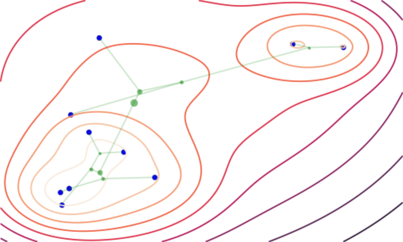
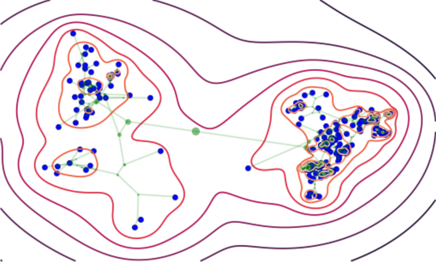
Figure 1: Independent samples from a time-marginalized coalescent (TMC) prior and two-dimensional Gaussian random walk likelihood model (10 and 300 leaves respectively). Contours in the plots correspond to posterior predictive density $r(z_{N+1}\,|\,z_{1:N},\tau)$. As the number of leaves grow, the predictive density grows more complex.

Hierarchical clustering is a flexible tool in exploratory data analysis as trees offer visual, interpretable summaries of data. Typically, algorithms for hierarchical clustering are either agglomerative (where data are recursively, greedily merged to form a tree from the bottom-up) or divisive (where data are recursively partitioned, forming a tree from the top-down). Bayesian nonparametric hierarchical clustering (BNHC) additionally incorporates uncertainty over tree structure by introducing a prior distribution over trees $r(\tau)$ and a likelihood model for data $r(z_{1:N}\,|\,\tau)$, with the goal of sampling the posterior distribution $r(\tau\,|\,z_{1:N})$.

In this paper, we focus on rooted binary trees with $N$ labeled leaves adorned with branch lengths, called phylogenies. Prior distributions over phylogenies often take the form of a stochastic generative process in which a tree is built with random merges, as in the Kingman coalescent (Kingman,, 1982), or random splits, as in the Dirichlet diffusion tree (Neal,, 2003). These nonparametric distributions have helpful properties, such as exchangeability, which enable efficient Bayesian inference. In this paper, we focus on the time-marginalized coalescent (TMC; Boyles and Welling,, 2012), which decouples the distribution over tree structure and branch length, a property that helps simplify inference down the line.

2.1.1 Time-marginalized coalescent (TMC)

The time-marginalized coalescent defines a prior distribution over phylogenies. A phylogeny $\tau=(V,E,T)$ is a directed rooted full binary tree, with vertex set $V$ and edges $E$, together with time labels $T:V\to[0,\,1]$ where we denote $t_{v}=T(v)$. The vertex set $V$ is partitioned into $N$ leaf vertices $V_{\text{leaf}}$ and $N-1$ internal vertices $V_{\text{int}}$, so that $V=V_{\text{int}}\cup V_{\text{leaf}}$, and we take $V_{\text{leaf}}=\{1,2,\ldots,N\}$ to simplify notation for identifying leaves with $N$ data points. The directed edges of the tree are encoded in the edge set $E\subset V_{\text{int}}\times V$, where we denote the root vertex as $v_{\text{root}}$ and for $v\in V\setminus\{v_{\text{root}}\}$ we denote the parent of $v$ as $\pi(v)=w$ where $(w,v)\in E$.

The TMC samples a random tree structure $(V,E)$ by a stochastic process in which the $N$ leaves are recursively merged uniformly at random until only one vertex is left. This process yields the probability mass function on valid $(V,E)$ pairs given by

$$r(V,E)=\frac{(N-1)!}{\prod_{v\in V_{\text{int}}}c(v)}\prod_{i=1}^{N-1}{i+1\choose 2}^{-1},$$ (1)

where $c(v)$ denotes the number of internal vertices in the subtree rooted at $v$. Given the tree structure, time labels are generated via the stick-breaking process

$$t_{v}=\begin{cases}0&v=v_{\text{root}},\\ 1&v\in V_{\text{leaf}},\\ t_{\pi(v)}-\beta_{v}(1-t_{\pi(v)})&v\in V_{\text{int}}\setminus\{v_{\text{root}}\},\end{cases}$$ (2)

where $\beta_{v}\stackrel{{\scriptstyle\mathrm{iid}}}{{\sim}}\mathrm{Beta}(a,b)$ for $v\in V$. These time labels encode a branch length $t_{v}-t_{\pi(v)}$ for each edge $e=(\pi(v),v)\in E$. We denote the overall density on phylogenies with $N$ leaves as $\mathrm{TMC}_{N}(\tau;a,b)$.

Finally, to connect the TMC prior to data in $\mathbb{R}^{d}$, we define a likelihood model $r(z_{1:N}\,|\,\tau)$ on $N$ data points, with $z_{n}$ corresponding to the leaf vertex $n\in V_{\text{leaf}}$. We use a Gaussian random walk (GRW), where for each vertex $v\in V$ a location $z_{v}\,|\,z_{\pi(v)}$ is sampled according to a Gaussian distribution centered at its parent’s location with variance equal to the branch length,

$$z_{v}\,|\,z_{\pi(v)}\sim\mathcal{N}(z_{\pi(v)},(t_{v}-t_{\pi(v)})I),\quad v\in V\setminus\{v_{\text{root}}\},$$

and we take $z_{v_{\text{root}}}\sim\mathcal{N}(0,I)$. As a result of this choice, we can exploit the Gaussian graphical model structure to efficiently marginalize out the internal locations $z_{v}$ associated with internal vertices $v\in V_{\text{int}}$ and evaluate the resulting marginal density $r(z_{1:N}\,|\,\tau)$. For details about this marginalization, please refer to Appendix C. The final overall density is written as

$$r(z_{1:N},\tau)=\mathrm{TMC}_{N}(\tau;a,b)r(z_{1:N}\,|\,\tau).$$ (3)

For further details and derivations related to the TMC, please refer to Boyles and Welling, (2012).

2.1.2 TMC posterior predictive density

The TMC with $N$ leaves and a GRW likelihood model can be a prior on a set of $N$ hierarchically-structured data, i.e. data that correspond to nodes with small tree distance should have similar location values. In addition, it also acts as a density from which we can sample new data. The posterior predictive density $r(z_{N+1}\,|\,z_{1:N},\tau)$ is easy to sample thanks to the exchangeability of the TMC.

To sample a new data point $z_{N+1}$, we select a branch (edge) and a time to attach a new leaf node. The probability $r(e_{N+1}\,|\,V,E)$ of selecting branch $e_{N+1}$ is proportional to the probability under the TMC prior of the tree with a new leaf attached to branch $e_{N+1}$. The density $r(t_{N+1}\,|\,e_{N+1},V,E)$ for a time label $t_{N+1}$ is determined by the stick-breaking process (see Appendix C for details). Both of these probabilities are easy to calculate and sample due to the exchangeability of the TMC.

The new location $z_{N+1}$ can be sampled from $r(z_{N+1}\,|\,e_{N+1},t_{N+1},\tau)$, which is the Gaussian distribution that comes out of the GRW likelihood model. Pictured in Figure 1 are samples from a TMC prior and GRW likelihood, where contours correspond to $r(z_{N+1}\,|\,z_{1:N},\tau)$. In addition to modeling hierarchical structure, the TMC is a flexible nonparametric density estimator.

2.1.3 TMC inference

The posterior distribution $r(\tau\,|\,z_{1:N})$ is analytically intractable due to the normalization constant $r(z_{1:N})$ involving a sum over all tree structures, but it can be approximately sampled via Markov chain Monte-Carlo (MCMC) methods. We utilize the Metropolis-Hastings algorithm with a subtree-prune-and-regraft (SPR) proposal distribution (Neal,, 2003). An SPR proposal picks a subtree uniformly at random from $\tau$ and detaches it. It is then attached back on the tree to a branch and time picked uniformly at random. The Metropolis-Hastings acceptance probability is efficient to compute because the joint density $r(\tau,z_{1:N})$ can be evaluated using belief propagation to marginalize the latent values at internal nodes of $\tau$, and many of the messages can be cached. See Appendix C for details.

2.2 Variational autoencoder

The variational autoencoder (VAE) is a generative model for a dataset $x_{1:N}$ wherein latent vectors $z_{1:N}$ are sampled from a prior distribution and then individually passed into a neural network observation model with parameters $\theta$,

$$\begin{split}z_{1:N}\sim p(z_{1:N}),\qquad x_{n}\,|\,z_{n}\sim p_{\theta}(x_{n}\,|\,z_{n}),\end{split}$$ (4)

We are interested in the posterior distribution $p(z_{n}\,|\,x_{n})$, which is not analytically tractable but can be approximated with a variational distribution $q_{\phi}(z_{n}\,|\,x_{n})$, typically a neural network that outputs parameters of a Gaussian distribution. The weights of the approximate posterior can be learned by optimizing the evidence-lower bound (ELBO),

$$\begin{split}\mathcal{L}[q]&\triangleq\mathbb{E}_{q}\left[\log\frac{p_{\theta}(x_{1:N},z_{1:N})}{\prod_{n}q_{\phi}(z_{n}\,|\,x_{n})}\right]\\ \end{split}$$ (5)

The parameters of the model, $\theta$ and $\phi$, are learned via stochastic gradient ascent on the ELBO, using the reparametrization trick for lower variance gradients (Kingma and Welling,, 2014; Rezende et al.,, 2014).

3 The TMC-VAE

The choice of prior distribution in the VAE significantly affects the autoencoder and resulting latent space. The default standard normal prior, which takes $z_{n}\stackrel{{\scriptstyle\mathrm{iid}}}{{\sim}}\mathcal{N}(0,I)$, acts as a regularizer on an otherwise unconstrained autoencoder, but can be restrictive and result in overpruning (Burda et al.,, 2015). Extremely flexible, learnable distributions like masked autoregressive flow (MAF) priors (Papamakarios et al.,, 2017) enable very rich latent spaces, but don’t encode any interpretable bias for organizing the latent space (except perhaps smoothness).

In this paper, we explore the TMC prior for the VAE, which could potentially strike a sweet spot between restrictive and flexible priors. We generate the latent values $z_{1:N}$ of a VAE according to the TMC prior, then generate observations $x_{1:N}$ using a neural network observation model,

$$\tau\sim\mathrm{TMC}_{N}(\tau;a,b),$$ (6)

$$z_{1:N}\,|\,\tau\sim r(z_{1:N}\,|\,\tau),\qquad x_{n}\,|\,z_{n}\sim p_{\theta}(x_{n}\,|\,z_{n}).$$ (7)

The TMC-VAE is a coherent generative process that captures discrete, interpretable structure in the latent space. A phylogeny not only has an intuitive inductive bias, but can be useful for exploratory data analysis and introspecting the latent space itself.

Consider doing inference in this model: first assume variational distributions $q_{\phi}(z_{n}\,|\,x_{n})$ (as in the VAE) and $q(\tau)$, which results in the ELBO,

$$\begin{split}\mathcal{L}[q]&=\mathbb{E}_{q}\left[\log\frac{p(\tau,z_{1:N},x_{1:N})}{q(\tau)\prod_{n}q(z_{n}\,|\,x_{n})}\right]\\ \end{split}$$ (8)

For fixed $q_{\phi}(z_{n}\,|\,x_{n})$, we can sample the optimal $q^{*}(\tau)$,

$$q^{*}(\tau)\propto\exp\{\mathbb{E}_{q}\left[\log p(\tau,z_{1:N},x_{1:N})\right]\}$$ (9)

Because $p(z_{1:N}\,|\,\tau)$ is jointly Gaussian (factorizing according to tree structure) and $q_{\phi}(z_{n}\,|\,x_{n})$ is Gaussian, expectations with respect to $z_{1:N}$ can move into $\log p(\tau,z_{1:N},x_{1:N})$. This enables sampling the expected joint likelihood $\mathbb{E}_{q}\left[\log p(\tau,z_{1:N})\right]$ using SPR Metropolis-Hastings. However, optimizing this ELBO is problematic. $p(z_{1:N}|\tau)$ does not factorize independently, so computing unbiased gradient estimates from minibatches is impossible and requires evaluating all the data. Furthermore, the TMC is limiting from a computational perspective. Since a phylogeny has as many leaves as points in the dataset, belief propagation over internal nodes of the tree slows down linearly as the size of the dataset grows. In addition, SPR proposals mix very slowly for large trees. We found these limitations make the model impractical for datasets of more than 1000 examples.

In the next section, we address these computational issues, while retaining the interesting properties of the TMC-VAE.

(a) TMC-VAE graphical model

(b) LORACs-VAE graphical model

(c) LORACs-VAE variational factors

Figure 2: Graphical models and variational approximations for TMC models described in the paper

4 LORACs prior for VAEs

In this section, we introduce a novel approximation to the TMC prior, which preserves many desirable properties like structure and interpretability, while being computationally viable. Our key idea is to use a set of learned inducing points as the leaves of the tree in the latent space, analogous to inducing-input approximations for Gaussian processes (Snelson and Ghahramani,, 2006). In this model, latent vectors $z_{1:N}$ are not directly hierarchically clustered, but are rather independent samples from the induced posterior predictive density of a TMC. We call this the Latent ORganization of Arboreal Clusters (LORACs, pronounced “lorax”) prior.

To define the LORACs prior $p(\tau,z_{1:N})$, we first define an auxiliary TMC distribution $r(\tau,s_{1:M})$ with $M$ leaf locations $s_{1:M}$. We treat $s_{1:M}$ as a set of learnable free parameters, and define the conditional $r(\tau\,|\,s_{1:M})$ as the LORACs prior on phylogenies $\tau$:

$$p(\tau;s_{1:M})\triangleq r(\tau\,|\,s_{1:M}).$$ (10)

That is, we choose the prior on phylogenies $\tau$ to be the posterior distribution of a TMC with pseudo-observations $s_{1:M}$. Next, we define the LORACs prior on locations $z_{n}\mid\tau$ as a conditionally independent draw from the predictive distribution $r(s_{M+1}\,|\,\tau,s_{1:M})$, writing the sampled attachment branch and time as $e_{n}$ and $t_{n}$, respectively:

$$p(e_{n},t_{n}\,|\,\tau)\triangleq r(e_{M+1}=e_{n},t_{M+1}=t_{n}\,|\,\tau),$$

$$p(z_{n}\,|\,e_{n},t_{n},\tau)\triangleq r(s_{M+1}=z_{n}\,|\,e_{n},t_{n},\tau,s_{1:M}).$$ (11)

To complete the model, we use an observation likelihood parameterized by a neural network, writing

$$x_{n}\,|\,z_{n}\sim p_{\theta}(x_{n}\,|\,z_{n}).$$ (12)

By using the learned inducing points $s_{1:M}$, we avoid the main difficulty of inference in the TMC-VAE of Section 3, namely the need to do inference over all $N$ points in the dataset. Instead, dependence between datapoints is mediated by the set of inducing points $s_{1:M}$, which has a size independent of $N$. As a result, with the LORACs prior, minibatch-based learning becomes tractable even for very large datasets. The quality of the approximation to the TMC-VAE can be tuned by adjusting the size of $M$.

However, this technique presents its own inference challenges. Sampling the optimal variational factor $q^{*}(\tau)$ is no longer an option as it was in the TMC-VAE:

$$\begin{split}q^{*}(\tau;s_{1:M})&\textstyle\propto\exp\{\mathbb{E}_{q}\left[\log p(\tau,z_{1:N},x_{1:N})\right]\}\\ &\textstyle\propto\exp\{\log p(\tau;s_{1:M})+\sum_{n}\mathbb{E}_{q}\left[p(z_{n}\,|\,e_{n},t_{n},\tau)\right]\}\\ &\textstyle\propto\exp\{\log\mathrm{TMC}_{N}(\tau;a,b)\\ &\textstyle\qquad\quad+\sum_{m=1}^{M}\log r(s_{m}\,|\,s_{1:m-1},\tau)\\ &\textstyle\qquad\quad+\sum_{n}\mathbb{E}_{q}\left[\log p(z_{n}\,|\,e_{n},t_{n},\tau)\right]\}.\end{split}$$ (13)

This term has a sum over $N$ expectations; therefore computing this likelihood for the purpose of MCMC would involve passing the entire dataset through a neural network. Furthermore, the normalizer for this likelihood is intractable, but necessary for computing gradients w.r.t $s_{1:M}$. We therefore avoid using the optimal $q^{*}(\tau;s_{1:M})$ and set $q(\tau;s_{1:M})$ to the prior. This has the additional computational advantage of cancelling out the $\mathbb{E}_{q}[\log p(\tau)]$ term in the ELBO, which also has an intractable normalizing constant. If the inducing points are chosen so that they contain most of the information about the hierarchical organization of the dataset, then the approximation $p(\tau\,|\,z)\approx r(\tau\,|\,s_{1:M})=p(\tau)$ will be reasonable.

We also fit the variational factors $q(e_{n})$, $q_{\xi}(t_{n}\,|\,e_{n},z_{n};s_{1:M})$, and $q_{\phi}(z_{n}\,|\,x_{n})$. The factor for attachment times, $q_{\xi}(t_{n}\,|\,e_{n},z_{n};s_{1:M})$, is a recognition network that outputs a posterior over attachment times for a particular branch. Since the $q(\tau;s_{1:M})$ and $p(\tau;s_{1:M})$ terms cancel out, we obtain the following ELBO (some notation suppressed for simplicity):

$$\begin{split}\mathcal{L}[q]&\triangleq\mathbb{E}_{q}\left[\log\frac{\prod_{n}p(e_{n},t_{n}\,|\,\tau)p(z_{n}\,|\,e_{n},t_{n},\tau)p(x_{n}\,|\,z_{n})}{\prod_{n}q(e_{n})q(t_{n}\,|\,e_{n},z_{n})q(z_{n}\,|\,x_{n})}\right].\end{split}$$ (14)

This ELBO can be optimized by first computing

$$q^{*}(e_{n})=\exp\left\{\mathbb{E}_{q}\left[\log p(e_{n}\,|\,t_{n},z_{n},\tau;s_{1:M})\right]\right\}$$ (15)

and computing gradients with respect to $\theta$, $s_{1:M}$, $\phi$, and $\xi$ using a Monte-Carlo estimate of the ELBO using samples from $q(\tau;s_{1:M})$, $q^{*}(e_{n})$, $q_{\phi}(z_{n}\,|\,x_{n})$, and $q_{\xi}(t_{n}\,|\,e_{n},z_{n};s_{1:M})$. The factor $q(\tau;s_{1:M})$ can be sampled using vanilla SPR Metropolis-Hastings. The detailed inference procedure can be found in Appendix C.

5 Related work

As mentioned above, LORACs connects various ideas in the literature, including Bayesian nonparametrics (Boyles and Welling,, 2012), inducing-point approximations (e.g.; Snelson and Ghahramani,, 2006; Tomczak and Welling,, 2018), and amortized inference (Kingma and Welling,, 2014; Rezende et al.,, 2014).

Also relevant is a recent thread of efforts to endow VAEs with the interpretability of graphical models (e.g.; Johnson et al.,, 2016; Lin et al.,, 2018). In this vein, Goyal et al., (2017) propose using a different Bayesian nonparametric tree prior, the nested Chinese restaurant process (CRP) (Griffiths et al.,, 2004), in a VAE. We chose to base LORACs on the TMC instead, as the posterior predictive distribution of an nCRP is a finite mixture, whereas the TMC’s posterior predictive distribution has more complex continuous structure. Another distinction is that Goyal et al., (2017) only consider learning from pretrained image features, whereas our approach is completely unsupervised.

6 Results

In this section, we analyze properties of the LORACs prior, focusing on qualitative aspects, like exploratory data analysis and interpretability, and quantitative aspects, like few-shot classification and information retrieval.

Experimental setup

We evaluated the LORACs prior on three separate datasets: dynamically binarized MNIST (LeCun and Cortes,, 2010), Omniglot (Lake et al.,, 2015), and CelebA (Liu et al.,, 2015). For all three experiments, we utilized convolutional/deconvolutional encoders/decoders and a 40-dimensional latent space (detailed architectures can be found in Appendix D). We used 200, 1000, and 500 inducing points for MNIST, Omniglot, and CelebA respectively with TMC parameters $a=b=2$. $q_{\xi}(t_{n}\,|\,e_{n},z_{n};s_{1:M})$ was a two-layer 500-wide neural network with ReLU activations that output parameters of a logistic-normal distribution over stick size and all parameters were optimized with Adam (Kingma and Ba,, 2015). Other implementation details can be found in Appendix D.

6.1 Qualitative results

A hierarchical clustering in the latent space offers a unique opportunity for interpretability and exploratory data analysis, especially when the data are images. Here are some methods for users to obtain useful data summaries and explore a dataset.

Visualizing inducing points

We first inspect the learned inducing points $s_{1:M}$ by passing them through the decoder. Visualized in Figure 3 are the 200 learned inducing points for MNIST. The inducing points are all unique and are cleaner than pseudo-input reconstructions from VampPrior (shown in Figure A.13). Inducing points can help summarize a dataset, as visualizations of the latent space indicate they spread out and cover the data (see Figure A.11). Inducing points are also visually unique and sensible in Omniglot and CelebA (see Figure A.14 and A.15).

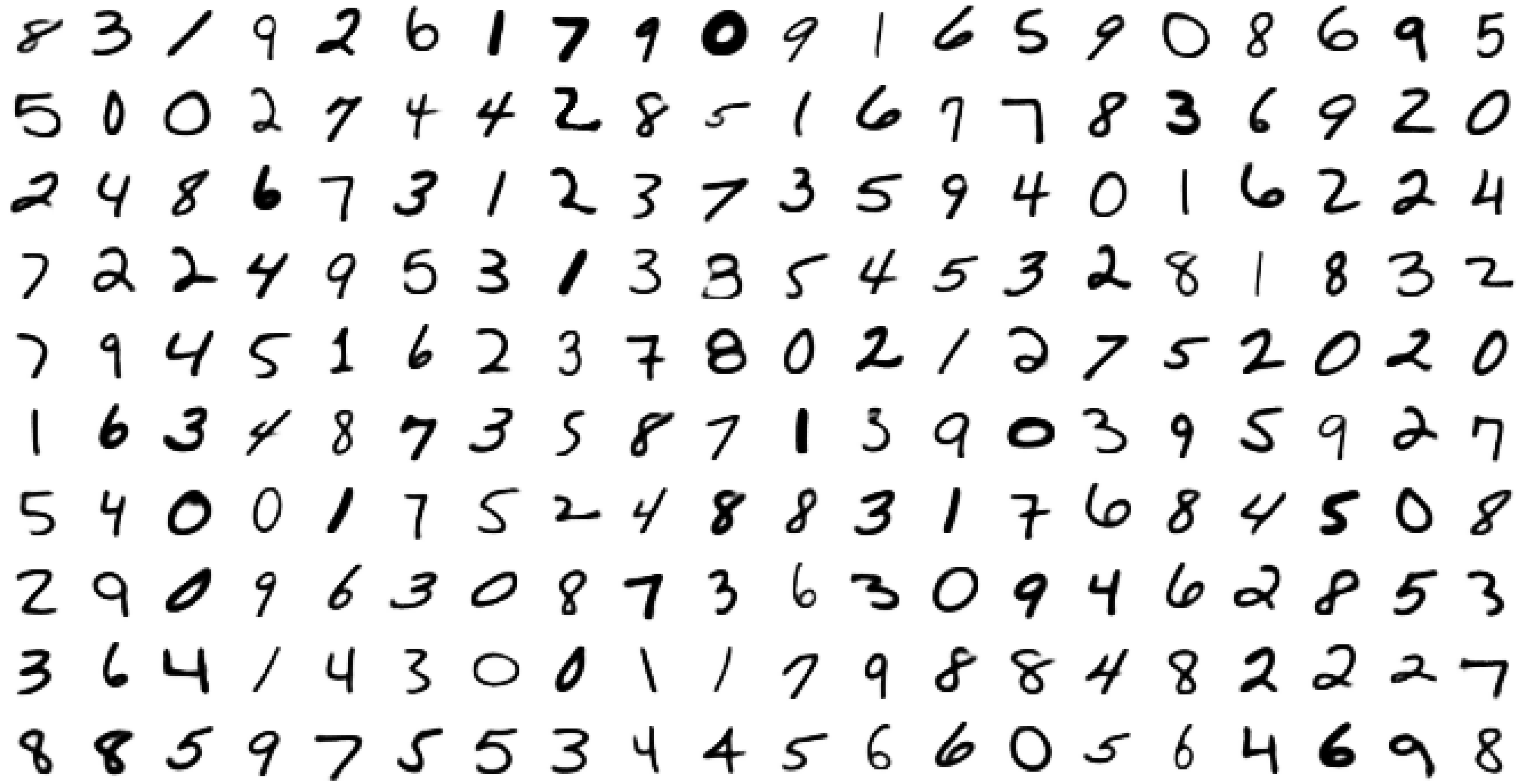
Figure 3: Learned inducing points for a LORACs(200) prior on MNIST.

Hierarchical clustering

We can sample $q(\tau;s_{1:M})$ to obtain phylogenies over the inducing points, and can visualize these clusterings using the decoded inducing points; subtrees from a sample in each dataset are visualized in Figure 4. In MNIST, we find large subtrees correspond to the discrete classes in the dataset. In Omniglot, subtrees sometimes correspond to language groups and letter shapes. In CelebA, we find subtrees sometimes correspond to pose or hair color and style.

We can further use the time at each internal node to summarize the data at many levels of granularity. Consider “slicing” the hierarchy at a particular time $t$ by taking every branch $(\pi(v),v)\in E$ with $t_{\pi(v)}\leq t<t_{v}$ and computing the corresponding expected Gaussian random walk value at time $t$. At times closer to zero, we slice fewer branches and are closer to the root of the hierarchy, so the value at the slice looks more like the mean of the data. In Figure 5, we visualize this process over a subset of the inducing points of CelebA. Visualizing the dataset in this way reveals cluster structure at different granularities and offers an evolutionary interpretation to the data, as leaves that coalesce more “recently” are likely to be closer in the latent space.

Although the hierarchical clustering is only over inducing points, we can still visualize where real data belong on the hierarchy by computing $q^{*}(e_{n})$ and attaching the data to the tree. By doing this for many points of data, and removing the inducing points from the tree, we obtain an induced hierarchical clustering.

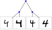
(a) MNIST

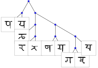
(b) Omniglot

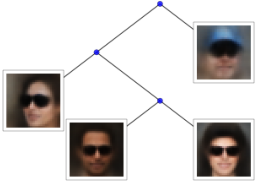
(c) CelebA

Figure 4: An example learned subtree from a sample of $q(\tau;s_{1:M})$ for each dataset. Leaves are visualized by passing inducing points throught the decoder.

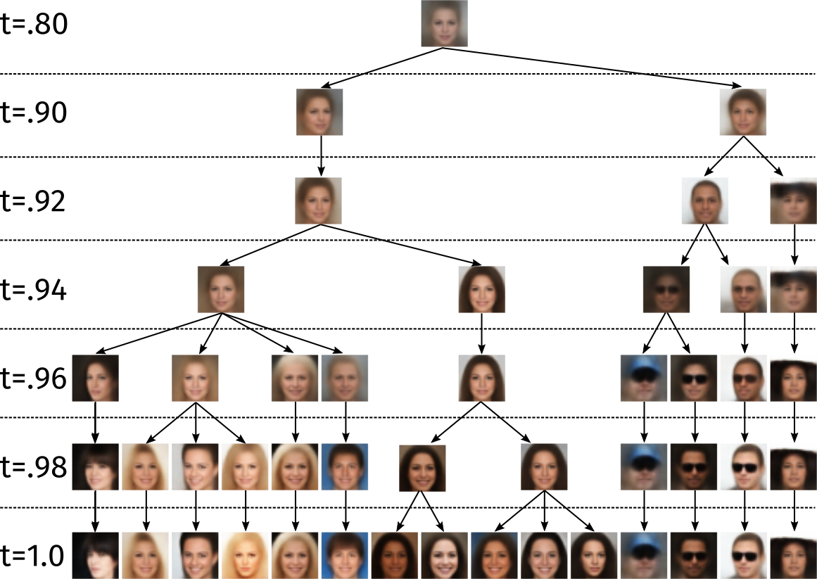
Figure 5: The evolution of a CelebA over a subset of inducing points. We create this visualization by taking slices of the tree at particular times and looking at the latent distribution at each of the sliced branches.

Generating samples

Having fit a generative model to our data, we can visualize samples from the model. Although we do not expect the samples to have fidelity and sharpness comparable to those from GANs or state-of-the-art decoding networks (Radford et al.,, 2015; Salimans et al.,, 2017), sampling with the LORACs prior can help us understand the latent space. To draw a sample from a TMC’s posterior predictive density, we first sample a branch and time, assigning the sample a place in the tree. This provides each generated sample a context, i.e., the branch and subtree it was generated from. However, learning a LORACs prior allows us to conditionally sample in a novel way. By restricting samples to a subtree, we can generate samples from the support of the posterior predictive density limited to that subtree. This enables conditional sampling at many levels of the hierarchy. We visualize examples of this in Figure 6 and Figure 7.

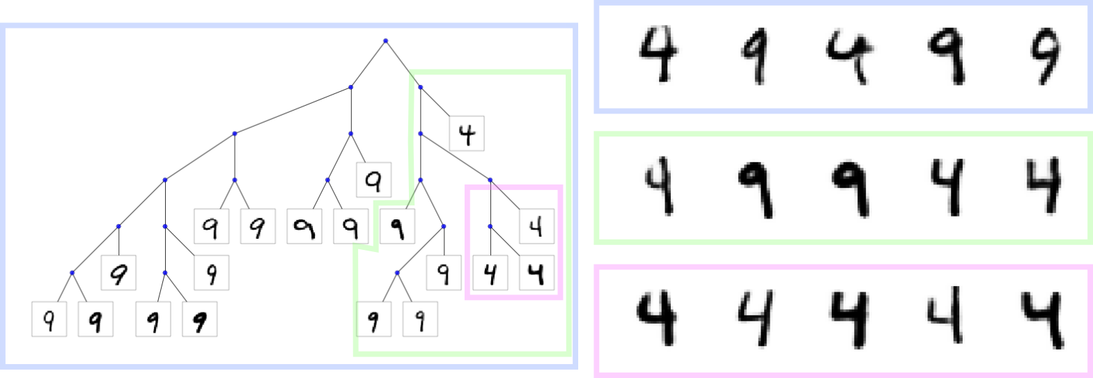
(a) MNIST

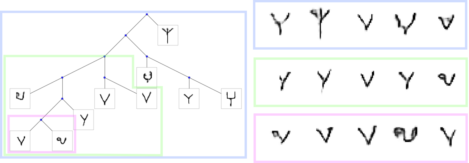
(b) Omniglot

Figure 6: Conditional samples from subtrees.

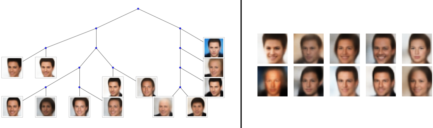
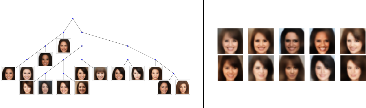
Figure 7: Samples from subtrees of CelebA.

6.2 Quantitative results

We ran experiments designed to evaluate the usefulness of the LORACs’s learned latent space for downstream tasks. We compare the LORACs prior against a set of baseline priors on three different tasks: few-shot classification, information retrieval, and generative modeling. Our datasets are dynamically binarized MNIST and Omniglot (split by instance) and our baselines are representations learned with the same encoder-decoder architecture and latent dimensionality but substituting the following prior distributions over $z$:

• No prior

• Standard normal prior

• VampPrior (Tomczak and Welling,, 2018) - 500 pseudo-inputs for MNIST, 1000 for Omniglot

• DVAE$\sharp$ (Vahdat et al.,, 2018) - latent vectors are 400-dimensional, formed from concatenating binary latents, encoder and decoder are two-layer feed-forward networks with ReLU nonlinearities

• Masked autoregressive flow (MAF; Papamakarios et al.,, 2017) - two layer, 512 wide MADE

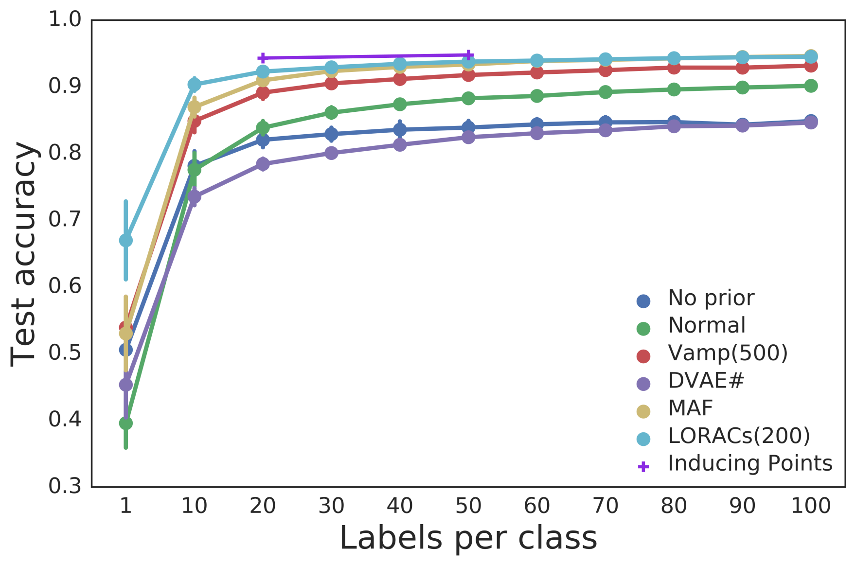
(a) MNIST

(b) Omniglot

Figure 8: Few-shot classification results

Few-shot classification

In this task, we train a classifier with varying numbers of labels and measure test accuracy. We pick equal numbers of labels per class to avoid imbalance and we use a logistic regression classifier trained to convergence to avoid adding unnecessary degrees of freedom to the experiment. We replicated the experiment across 20 randomly chosen label sets for MNIST and 5 for Omniglot. The test accuracy on these datasets is visualized in Figure 8. For MNIST, we also manually labeled inducing points and found that training a classifier on 200 and 500 inducing points achieved significantly better test accuracy than randomly chosen labeled points, hinting that the LORACs prior has utility in an active learning setting.

The representations learned with the LORACs  consistently achieve better accuracy, though in MNIST, LORACs prior and MAF reach very similar test accuracy at 100 labels per class. The advantage of the LORACs prior is especially clear in Omniglot (Table B.3 and Table B.4 contain the exact numbers). We believe our advantage in this task comes from ability of the LORACs prior to model discrete structure. TSNE visualizations in Figure 9 and Figure A.10 indicate clusters are more concentrated and separated with the LORACs prior than with other priors, though TSNE visualizations should be taken with a grain of salt.

(a) Normal prior

(b) LORACs(200) prior

Figure 9: TSNE visualizations of the latent space of the MNIST test set with different priors, color-coded according to class. LORACs prior appears to learn a space with more separated, concentrated clusters.

Information retrieval

We evaluated the meaningfulness of Euclidean distances in the learned latent space by measuring precision-recall when querying the test set. We take each element of the test set and sort all other members according to their $L_{2}$ distance in the latent space. From this ranking, we produce precision-recall curves for each of the query and plot the average precision-recall over the entire test set in Figure B.16. We also report the area-under-the-curve (AUC) measure for each of these curves in Table 1.

AUC numbers for Omniglot are low across the board because of the large number of classes and low number of instances per class. However, in both datasets the LORACs prior consistently achieves the highest AUC, especially with MNIST. The LORACs prior encourages tree-distance to correspond to squared Euclidean distance, as branch lengths in the tree are variances in a Gaussian likelihoods. We thus suspect distances in a LORACs prior latent space to be more informative and better for information retrieval.

Held-out log-likelihood

We estimate held-out log-likelihoods for the four VAEs we trained with comparable architectures and different priors. (We exclude DVAE$\sharp$ since its architecture is substantially different, and the classical autoencoder since it lacks generative semantics.) We use 1000 importance-weighted samples (Burda et al.,, 2015) to estimate held-out log-likelihood, and report the results in Table 2. We find that, although LORACs outperforms the other priors on downstream tasks, it only achieves middling likelihood numbers. This result is consistent with the findings of Chang et al., (2009) that held-out log-likelihood is not necessarily correlated with interpretability or usefulness for downstream tasks.

Prior	MNIST	Omniglot
No prior	0.429	0.078
Normal	0.317	0.057
VAMP	0.502	0.063
DVAE#	0.490	0.024
MAF	0.398	0.070
LORACs	0.626	0.087

Table 1: Averaged precision-recall AUC on MNIST/Omniglot test datasets

Prior	MNIST	Omniglot
Normal	-83.789	-89.722
MAF	-80.121	-86.298
Vamp	-83.0135	-87.604
LORACs	-83.401	-87.105

Table 2: MNIST/Omniglot test log-likelihoods

7 Discussion

Learning discrete, hierarchical structure in a latent space opens a new opportunity: interactive deep unsupervised learning. User-provided constraints have been used in both flat and hierarchical clustering (Wagstaff and Cardie,, 2000; Awasthi et al.,, 2014), so an interesting follow up to this work would be incorporating constraints into the LORACs  prior, as in Vikram and Dasgupta, (2016), which could potentially enable user-guided representation learning.

 

The LORACs prior for VAEs: Letting the Trees Speak for the Data - Supplement

 

Appendix A Additional visualizations

(a) Normal prior

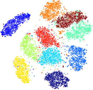
(b) No prior

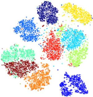
(c) Vamp(500) prior

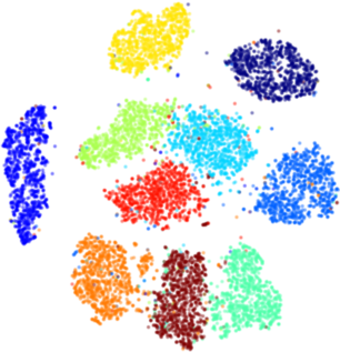
(d) MAF prior

(e) LORACs(200) prior

Figure A.10: TSNE visualizations of the latent space of the MNIST test set with various prior distributions, color-coded according to class.

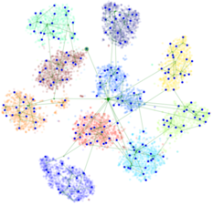
Figure A.11: A TSNE visualization of the latent space for the TMC(200) model with inducing points and one sample from $q(\tau;s_{1:M})$ plotted. Internal nodes are visualized by computing their expected posterior values, and branches are plotted in 2-d space.

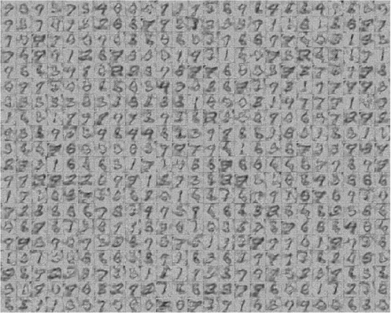
Figure A.12: MNIST VampPrior learned pseudo-inputs.

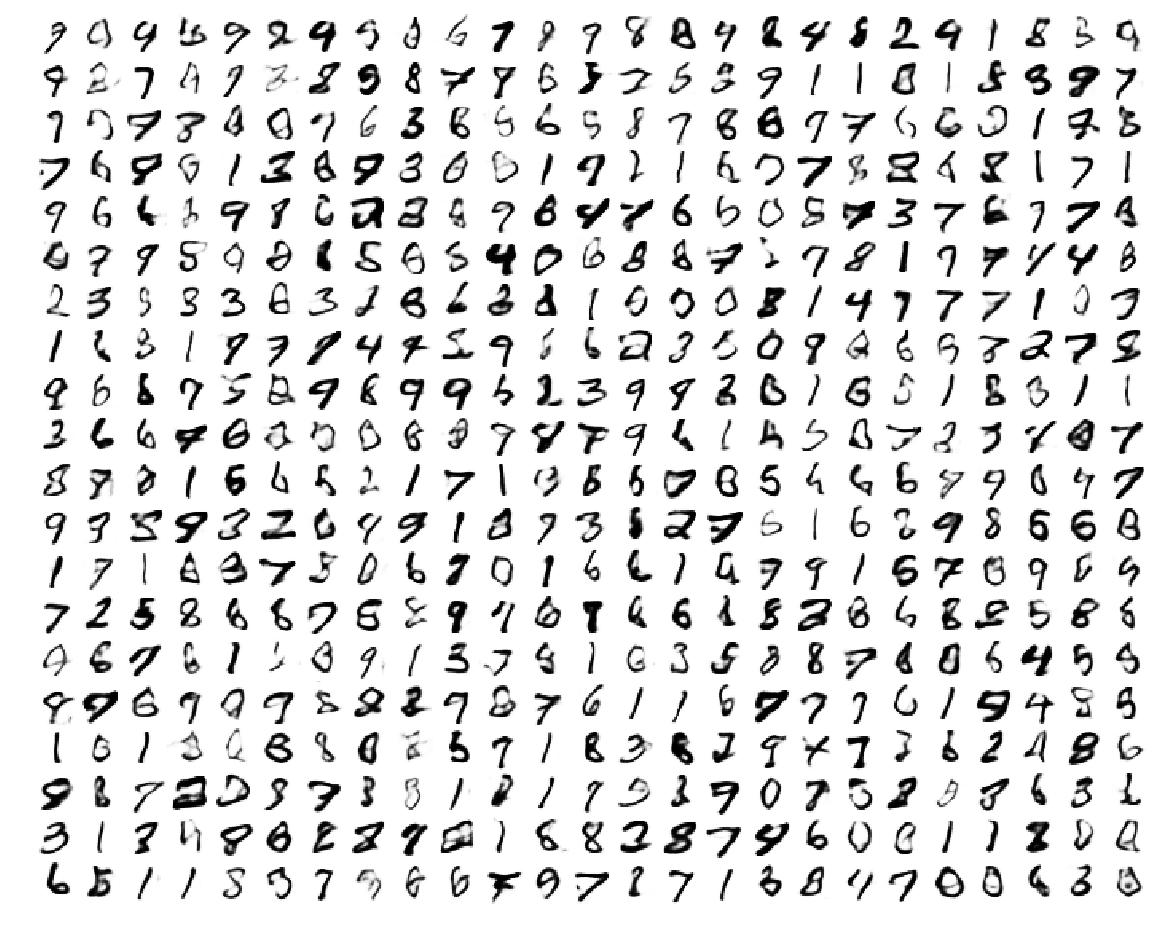
Figure A.13: MNIST VampPrior reconstructed pseudo-inputs obtained by deterministically encoding and decoding each pseudo-input.

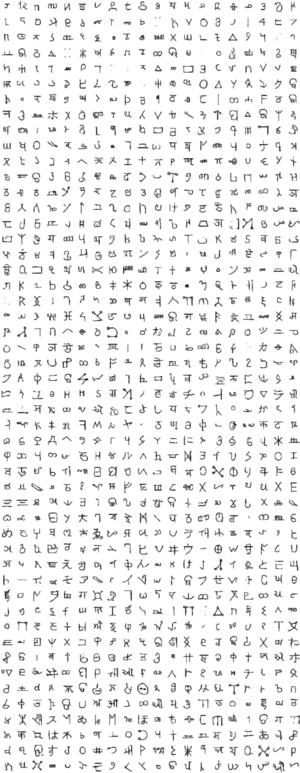
Figure A.14: Omniglot learned inducing points.

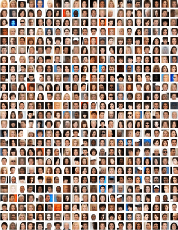
Figure A.15: CelebA learned inducing points.

Appendix B Empirical results

Labels per class	1	10	20	30	40	50	60	70	80	90	100
No prior	$0.506\pm 0.095$	$0.781\pm 0.045$	$0.820\pm 0.023$	$0.829\pm 0.020$	$0.836\pm 0.026$	$0.839\pm 0.021$	$0.844\pm 0.017$	$0.846\pm 0.017$	$0.847\pm 0.015$	$0.843\pm 0.015$	$0.848\pm 0.014$
Normal	$0.396\pm 0.076$	$0.775\pm 0.051$	$0.838\pm 0.020$	$0.861\pm 0.016$	$0.874\pm 0.011$	$0.883\pm 0.011$	$0.886\pm 0.011$	$0.892\pm 0.010$	$0.896\pm 0.010$	$0.899\pm 0.011$	$0.901\pm 0.008$
Vamp(500)	$0.539\pm 0.094$	$0.849\pm 0.035$	$0.891\pm 0.019$	$0.905\pm 0.013$	$0.911\pm 0.016$	$0.918\pm 0.012$	$0.921\pm 0.009$	$0.925\pm 0.008$	$0.929\pm 0.007$	$0.928\pm 0.005$	$0.932\pm 0.005$
DVAE#	$0.453\pm 0.101$	$0.735\pm 0.027$	$0.784\pm 0.017$	$0.801\pm 0.012$	$0.813\pm 0.013$	$0.824\pm 0.014$	$0.830\pm 0.012$	$0.835\pm 0.011$	$0.841\pm 0.007$	$0.842\pm 0.007$	$0.846\pm 0.008$
MAF	$0.530\pm 0.113$	$0.869\pm 0.029$	$0.910\pm 0.012$	$0.923\pm 0.012$	$0.930\pm 0.007$	$0.933\pm 0.010$	$0.938\pm 0.008$	$0.940\pm 0.008$	$0.942\pm 0.006$	$0.944\pm 0.006$	$\mathbf{0.946\pm 0.005}$
LORACs(200)	$\mathbf{0.670\pm 0.120}$	$\mathbf{0.903\pm 0.019}$	$\mathbf{0.923\pm 0.011}$	$\mathbf{0.929\pm 0.009}$	$\mathbf{0.934\pm 0.006}$	$\mathbf{0.938\pm 0.004}$	$\mathbf{0.939\pm 0.005}$	$\mathbf{0.941\pm 0.004}$	$\mathbf{0.943\pm 0.004}$	$\mathbf{0.944\pm 0.003}$	$0.945\pm 0.003$

Table B.3: MNIST few-shot classification results.

Labels per class	1	2	5	10	15
No prior	$0.140\pm 0.012$	$0.179\pm 0.008$	$0.225\pm 0.006$	$0.252\pm 0.009$	$0.290\pm 0.001$
Normal	$0.107\pm 0.007$	$0.134\pm 0.010$	$0.187\pm 0.008$	$0.246\pm 0.006$	$0.285\pm 0.000$
Vamp(1000)	$0.116\pm 0.011$	$0.148\pm 0.009$	$0.210\pm 0.003$	$0.270\pm 0.005$	$0.300\pm 0.000$
DVAE#	$0.042\pm 0.004$	$0.060\pm 0.006$	$0.091\pm 0.003$	$0.121\pm 0.001$	$0.141\pm 0.000$
MAF	$0.096\pm 0.008$	$0.129\pm 0.006$	$0.177\pm 0.010$	$0.222\pm 0.007$	$0.237\pm 0.002$
LORACs(1000)	$\mathbf{0.173\pm 0.005}$	$\mathbf{0.236\pm 0.005}$	$\mathbf{0.330\pm 0.008}$	$\mathbf{0.403\pm 0.006}$	$\mathbf{0.441\pm 0.000}$

Table B.4: Omniglot few-shot classification results.

# of inducing points	200	500
	0.9428	0.9474

Table B.5: MNIST few-shot classification with labeled inducing points.

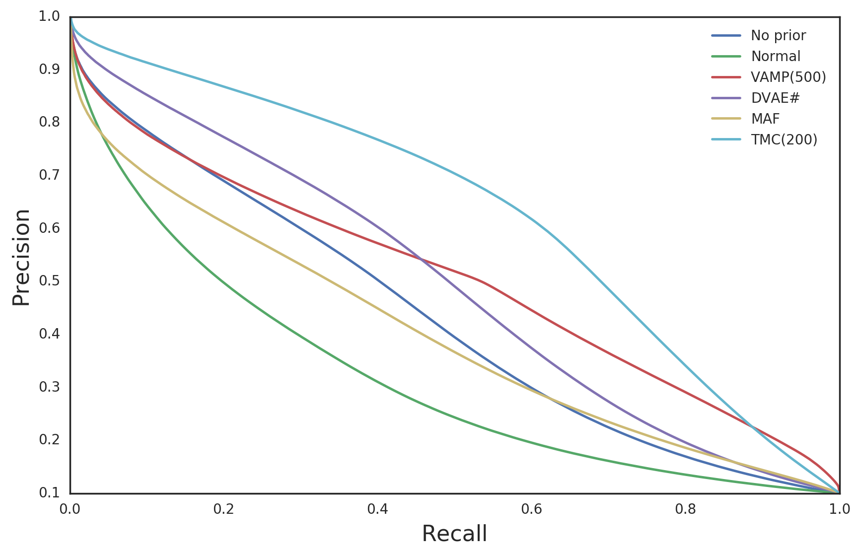
(a) MNIST

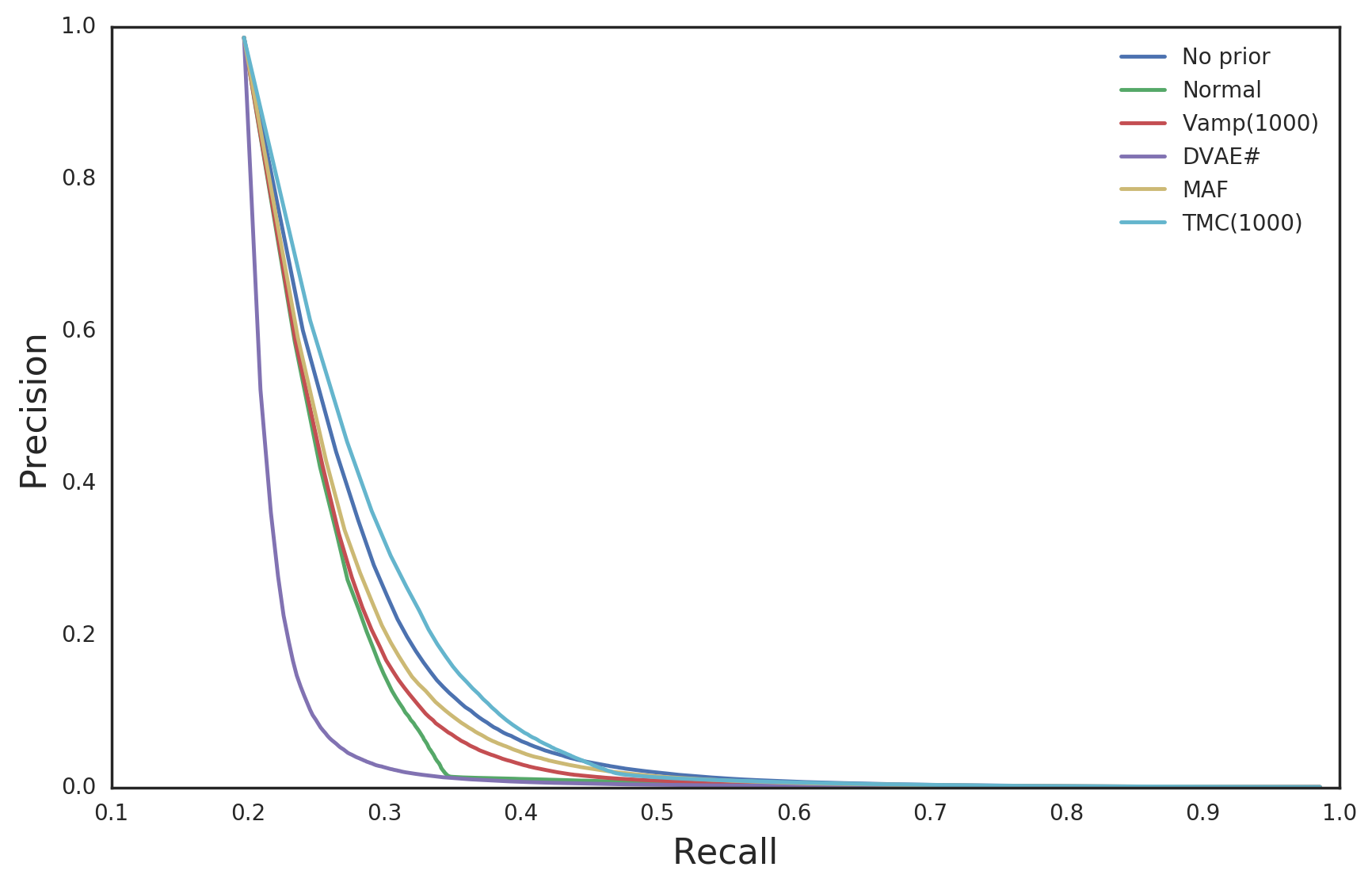
(b) Omniglot

Figure B.16: Averaged precision-recall curves over test datasets.

Appendix C Algorithm details

C.1 Stick breaking process

Consider inserting a node $N+1$ into the tree in between vertices $u$ and $v$ such that $t_{v}>t_{u}$, creating branch $e_{N+1}$. The inserted node has time $t_{N+1}$ with probability according to the stick breaking process, i.e.

$$\textstyle r(t_{N+1}\,|\,e_{N+1},V,E)=\mathrm{Beta}\left(\frac{t_{v}-t_{N+1}}{1-t_{N+1}};a,b\right)\mathrm{Beta}\left(\frac{t_{N+1}-t_{u}}{1-t_{u}};a,b\right).$$ (C.16)

C.2 Belief propagation in TMCs

The TMC is at the core of the LORACs  prior. Recall that the TMC is a prior over phylogenies $\tau$, and after attaching a Gaussian random walk (GRW), we obtain a distribution over $N$ vectors in $\mathbb{R}^{d}$, corresponding to the leaves, $r(z_{1:N}\,|\,\tau)$. However, the GRW samples latent vectors at internal nodes $z_{V_{\text{int}}}$. Rather than explicitly representing these values, in this work we marginalize them out, i.e.

$$r(z_{1:N}\,|\,\tau)=\int r(z_{1:N}\,|\,z_{V_{\text{int}}},\tau)p(z_{V_{\text{int}}}\,|\,\tau)dz_{V_{\text{int}}}$$ (C.17)

This marginalization process can be done efficiently, because our graphical model is tree-shaped and all nodes have Gaussian likelihoods. Belief propagation is a message-passing framework for marginalization and we utilize message-passing for several TMC inference queries. The main queries we are interested in are:

1. $r(z_{1:N},\tau)$ - for the purposes of MCMC, we are interested in computing the joint likelihood of a set of observed leaf values and a phylogeny.

2. $r(z_{n}\,|\,z_{\backslash n},\tau)$ - this query computes the posterior density over one leaf given all the others; we use this distribution when computing the posterior predictive density of a TMC.

3. $\nabla_{z_{\backslash n}}r(z_{n}\,|\,z_{\backslash n},\tau)$ - this query is the gradient of the predictive density of a single leaf with respect to the values at all other leaves. This query is used when computing gradients of the ELBO w.r.t $s_{1:M}$ in the LORACs prior.

Message passing

Message passing treats the tree as an undirected graph. We first pick start node $v_{\text{start}}$ and request messages from each of $v_{\text{start}}$’s neighbors.

Message passing is thereafter defined recursively. When a node $v$ has requested messages from a source node $s$, it thereafter requests messages from all its neighbors but $s$. The base case for this recursion is a leaf node $v_{n}$, which returns a message with the following contents:

$$\nu_{n}=\bm{0};\quad\mu_{n}=z_{n};\quad\log Z_{n}=0;\quad\nabla_{\nu_{n}}(\nu)=\bm{1};\quad\nabla_{\nu_{n}}(\mu)=\bm{0};\quad\nabla_{\mu_{n}}(\mu)=\bm{1}$$ (C.18)

where bold numbers $\bm{0}\triangleq(0,\ldots,0)^{\top}$ and $\bm{1}\triangleq(1,\ldots,1)^{\top}$ denote vectors obtained by repeating a scalar $d$ times.

In the recursive case, consider being at a node $i$ and receiving a set of messages from its neighbors $M$.

$$\begin{split}\nu_{i}=\frac{1}{\sum_{m\in M}\frac{1}{\nu_{m}+e_{im}}};\quad\mu_{i}=v_{i}\sum_{m\in M}\frac{\mu_{m}}{\nu_{m}+e_{im}}\\ \end{split}$$ (C.19)

where $e_{im}$ is the length of the edge between nodes $i$ and $m$. These messages are identical to those used in Boyles and Welling, (2012).

Additionally, our messages include gradients w.r.t. every leaf node downstream of the message. We update each of these gradients when computing the new message and pass them along to the source node. Gradients with respect to one of these nodes $j$ are calculated as

$$\begin{split}\nabla_{\nu_{j}}(\nu)&=\nabla_{\nu_{j}}\nu_{i}\\ \nabla_{\nu_{j}}(\mu)&=\nabla_{\nu_{j}}\mu_{i}\\ \nabla_{\mu_{j}}(\mu)&=\nabla_{\mu_{j}}\mu_{i}\\ \end{split}$$ (C.20)

The most complicated message is the $\log Z_{i}$ message, which depends on the number of incoming messages. $v_{\text{start}}$ gets three incoming messages, all other nodes get only two. Consider two messages from nodes $v_{k}$ and $v_{l}$:

$$\begin{split}\Sigma_{i}&\triangleq(\nu_{k}+e_{ik}+\nu_{l}+e_{il})I\\ \log Z_{i}&=-\frac{1}{2}\|\mu_{k}-\mu_{l}\|^{2}_{\Sigma_{i}}-\frac{1}{2}\left(\log|\Sigma_{i}|_{d}\log 2\pi\right)\end{split}$$ (C.21)

For three messages from nodes $v_{k}$, $v_{l}$, and $v_{m}$:

$$\begin{split}\Sigma_{i}&\triangleq\left((\nu_{k}+e_{ik})(\nu_{l}+e_{il})+(\nu_{l}+e_{il})(\nu_{m}+e_{im})+(\nu_{m}+e_{im})(\nu_{k}+e_{ik})\right)I\\ \log Z_{i}&=-\frac{1}{2}\left((\nu_{m}+e_{im})\|\mu_{k}-\mu_{l}\|^{2}_{\Sigma_{i}}+(\nu_{k}+e_{ik})\|\mu_{l}-\mu_{m}\|^{2}_{\Sigma_{i}}+(\nu_{l}+e_{il})\|\mu_{m}-\mu_{k}\|^{2}_{\Sigma_{i}}\right)-\frac{1}{2}\log|\Sigma_{i}|-\log 2\pi\end{split}$$ (C.22)

With these messages, we can answer all the aforementioned inference queries.

1. We can begin message passing at any internal node and compute: $\log r(z_{1:N},\tau)=\sum_{v\in V}\log Z_{v}$

2. We start message passing at $v_{n}$. $r(z_{n}\,|\,z_{\backslash n},\tau)$ is a Gaussian with mean $\mu_{n}$ and variance $\nu_{n}$.

3. $\nabla_{z_{\backslash n}}r(z_{n}\,|\,z_{\backslash n},\tau)$ is $\nabla_{z_{\backslash n}}\mathcal{N}(z_{n}\,|\,\mu_{n},\nu_{n}I)$, which in turn utilizes gradients sent via message passing.

Implementation

We chose to implement the TMC and message passing in Cython because we found raw Python to be too slow due to function call and type-checking overhead. Furthermore, we used diagonal rather than scalar variances in the message passing implementation to later support diagonal variances handed from the variational posterior over $z_{n}$.

C.3 Variational inference for the LORACs prior

The LORACs  prior involves first sampling a tree from the posterior distribution over TMCs with $s_{1:M}$ as leaves. We then sample a branch and time for each data $z_{n}$ according to the posterior predictive distribution described in subsection 2.1. We then sample a $z_{n}$ from the distribution induced by the GRW likelihood model. Finally, we pass the sampled $z_{n}$ through the decoder.

$$\begin{split}\tau&\sim p(\tau;s_{1:M})\\ e_{n},t_{n}&\sim p(e_{n},t_{n}|\tau)\\ z_{n}|e_{n},t_{n},\tau&\sim p(z_{n}|e_{n},t_{n},\tau;s_{1:M})\triangleq r(s_{M+1}=z_{n}|e_{n},t_{n},\tau)\\ x_{n}|z_{n}&\sim p_{\theta}(x_{n}|z_{n})\end{split}$$ (C.23)

Consider sampling the optimal $q^{*}(\tau;s_{1:M})$.

$$\begin{split}q^{*}(\tau;s_{1:M})&\propto\exp\{\mathbb{E}_{q}\left[\log p(\tau,z_{1:N},x_{1:N})\right]\}\\ &\propto\exp\{\log p(\tau;s_{1:M})+\sum_{n}\mathbb{E}_{q}\left[p(z_{n}|e_{n},t_{n},\tau)\right]\}\\ &\propto\exp\{\log\mathrm{TMC}_{N}(\tau;a,b)+\sum_{m=1}^{M}\log r(s_{m}|s_{1:m-1},\tau)\\ &+\sum_{n}\mathbb{E}_{q}\left[\log p(z_{n}|e_{n},t_{n},\tau)\right]\}\\ \end{split}$$ (C.24)

We set $q(\tau;s_{1:M})=r(\tau\,|\,s_{1:M})$. We use additional variational factors $q(e_{n})$, $q_{\xi}(t_{n}|e_{n},z_{n};s_{1:M})$, and $q_{\phi}(z_{n}|x_{n})$. $q_{\xi}(t_{n}|e_{n},z_{n};s_{1:M})$ is a recognition network that outputs the attach time for a particular branch. Since the $q(\tau;s_{1:M})$ and $p(\tau;s_{1:M})$ terms cancel out, we obtain the following ELBO.

$$\begin{split}\mathcal{L}[q]&\triangleq\mathbb{E}_{q}\left[\log\frac{\prod_{n}p(e_{n},t_{n}|\tau)p(z_{n}|e_{n},t_{n},\tau;s_{1:M})p_{\theta}(x_{n}|z_{n})}{\prod_{n}q(e_{n})q_{\xi}(t_{n}|e_{n},z_{n};s_{1:M})q_{\phi}(z_{n}|x_{n})}\right]\\ \end{split}$$ (C.25)

Inference procedure

In general, $q(\tau;s_{1:M})$ can be sampled using vanilla SPR Metropolis-Hastings, so samples from this distribution are readily available.

For each data in the minibatch $x_{n}$, we pass it through the encoder to obtain $q(z_{n}|x_{n})$. We then compute

$$q^{*}(e_{n})=\exp\left\{\mathbb{E}_{q}\left[\log p(e_{n}|t_{n},z_{n},\tau;s_{1:M})\right]\right\}$$ (C.26)

This quantity is computed by looping over every branch $b$ of a sample from $q(\tau)$, storing incoming messages at each node, passing the $\mu$ and $\nu$ and a sample from $q(z_{n}|x_{n})$ into $q_{\xi}(t_{n}|e_{n},s_{1:M},z_{n})$, outputting a logistic-normal distribution over times for that branch. We sample that logistic normal to obtain a time $t$ to go with branch $b$. We can then compute the log-likelihood of $z_{n}$ if it were to attach to $b$ and $t$, using TMC inference query #2. This log-likelihood is added to the TMC prior log-probability of the branch being selected to obtain a joint probability $\mathbb{E}_{q}\left[\log p(e_{n})p(t_{n})p(z_{n}|e_{n},t_{n},\tau;s_{1:M})\right]$ over the branch. After doing this for every branch, we normalize the joint likelihoods to obtain the optimal categorical distribution over every branch for $z_{n}$, $q^{*}(e_{n})$. We then sample this distribution to obtain an attach location and time $e_{n},t_{n}$ for each data in the minibatch.

The next stage is to compute gradients w.r.t. to the learnable parameters of the model ($\theta$, $s_{1:M}$, $\phi$, and $\xi$). In the process of calculating $q^{*}(e_{n})$, we have obtained samples from its corresponding $q_{\xi}(t_{n}|e_{n},z_{n},\tau;s_{1:M})$ and $q(z_{n}|x_{n})$. We plug these into the ELBO and can compute gradients via automatic differentiation w.r.t. $\phi$, $\theta$, and $\xi$. Computing gradients w.r.t. $s_{1:M}$ is more tricky. We first examine the ELBO.

$$\mathcal{L}[q]=\mathbb{E}_{q}\left[\log\frac{\prod_{n}p(e_{n}|\tau)p(t_{n})p(z_{n}|e_{n},t_{n},\tau;s_{1:M})p_{\theta}(x_{n}|z_{n})}{\prod_{n}q(e_{n})q_{\xi}(t_{n}|e_{n},z_{n};s_{1:M})q_{\phi}(z_{n}|x_{n})}\right]$$ (C.27)

Consider the gradient of the ELBO with respect to $s_{1:M}$.

$$\begin{split}\nabla_{s_{1:M}}\mathcal{L}[q]&=\nabla_{s_{1:M}}\mathbb{E}_{q}\left[\log\frac{\prod_{n}p(e_{n}|\tau)p(t_{n})p(z_{n}|e_{n},t_{n},\tau;s_{1:M})p_{\theta}(x_{n}|z_{n})}{\prod_{n}q(e_{n})q_{\xi}(t_{n}|e_{n},z_{n};s_{1:M})q_{\phi}(z_{n}|x_{n})}\right]\\ &=\nabla_{s_{1:M}}\sum_{\tau}q(\tau;s_{1:M})\mathbb{E}_{q}\left[\log\frac{\prod_{n}p(e_{n}|\tau)p(t_{n})p(z_{n}|e_{n},t_{n},\tau;s_{1:M})p_{\theta}(x_{n}|z_{n})}{\prod_{n}q(e_{n})q_{\xi}(t_{n}|e_{n},z_{n};s_{1:M})q_{\phi}(z_{n}|x_{n})}\right]\\ &=\sum_{\tau}q(\tau;s_{1:M})\nabla_{s_{1:M}}\mathbb{E}_{q}\left[\log\frac{\prod_{n}p(e_{n}|\tau)p(t_{n})p(z_{n}|e_{n},t_{n},\tau;s_{1:M})p_{\theta}(x_{n}|z_{n})}{\prod_{n}q(e_{n})q_{\xi}(t_{n}|e_{n},z_{n};s_{1:M})q_{\phi}(z_{n}|x_{n})}\right]\\ &+\sum_{\tau}\left(\nabla_{s_{1:M}}q(\tau;s_{1:M})\right)\mathbb{E}_{q}\left[\log\frac{\prod_{n}p(e_{n}|\tau)p(t_{n})p(z_{n}|e_{n},t_{n},\tau;s_{1:M})p_{\theta}(x_{n}|z_{n})}{\prod_{n}q(e_{n})q_{\xi}(t_{n}|e_{n},z_{n};s_{1:M})q_{\phi}(z_{n}|x_{n})}\right]\\ &=\sum_{\tau}q(\tau;s_{1:M})\nabla_{s_{1:M}}\mathbb{E}_{q}\left[\log\frac{\prod_{n}p(e_{n}|\tau)p(t_{n})p(z_{n}|e_{n},t_{n},\tau;s_{1:M})p_{\theta}(x_{n}|z_{n})}{\prod_{n}q(e_{n})q_{\xi}(t_{n}|e_{n},z_{n};s_{1:M})q_{\phi}(z_{n}|x_{n})}\right]\\ &+\sum_{\tau}\left(q(\tau;s_{1:M})\nabla_{s_{1:M}}\log q(\tau;s_{1:M})\right)\mathbb{E}_{q}\left[\log\frac{\prod_{n}p(e_{n}|\tau)p(t_{n})p(z_{n}|e_{n},t_{n},\tau;s_{1:M})p_{\theta}(x_{n}|z_{n})}{\prod_{n}q(e_{n})q_{\xi}(t_{n}|e_{n},z_{n};s_{1:M})q_{\phi}(z_{n}|x_{n})}\right]\\ &=\mathbb{E}_{q(\tau)}\left[\nabla_{s_{1:M}}\mathbb{E}_{q}\left[\log\frac{\prod_{n}p(e_{n}|\tau)p(t_{n})p(z_{n}|e_{n},t_{n},\tau;s_{1:M})p_{\theta}(x_{n}|z_{n})}{\prod_{n}q(e_{n})q_{\xi}(t_{n}|e_{n},z_{n};s_{1:M})q_{\phi}(z_{n}|x_{n})}\right]\right.\\ &+\left.\nabla_{s_{1:M}}\log q(\tau;s_{1:M})\mathbb{E}_{q}\left[\log\frac{\prod_{n}p(e_{n}|\tau)p(t_{n})p(z_{n}|e_{n},t_{n},\tau;s_{1:M})p_{\theta}(x_{n}|z_{n})}{\prod_{n}q(e_{n})q_{\xi}(t_{n}|e_{n},z_{n};s_{1:M})q_{\phi}(z_{n}|x_{n})}\right]\right]\\ &=\mathbb{E}_{q}\left[\nabla_{s_{1:M}}\left(-\log q(e_{n})-\log q(t_{n}\,|\,z_{n},e_{n},\tau;s_{1:M})+\log p(z_{n}\,|\,e_{n},t_{n},\tau;s_{1:M})\right)\right]\\ &+\mathbb{E}_{q}\left[\nabla_{s_{1:M}}\left(\log q(\tau)+\log q(e_{n})\right)\log\frac{p(e_{n}|\tau)}{q(e_{n})}\frac{p(z_{n}\,|\,z_{n},e_{n},t_{n},\tau;s_{1:M})}{q(t_{n}\,|\,z_{n},e_{n},\tau;s_{1:M})}\right]\end{split}$$ (C.28)

In the last step, we expand out expectation over $e_{n}$ and then pass the derivative through like we did for $\tau$. The gradients w.r.t. $q(e_{n})$ are zero, since $q^{*}(e_{n})$ is a partial optimum of the ELBO and we are left with:.

$$\begin{split}\nabla_{s_{1:M}}\mathcal{L}[q]&=\mathbb{E}_{q}\left[\nabla_{s_{1:M}}\log p(z_{N}|e_{n},t_{n},\tau;s_{1:M})\right]-\mathbb{E}_{q}\left[\log q(t_{n}\,|\,z_{n},e_{n},\tau;s_{1:M})\right]\\ &+\mathbb{E}_{q}\left[\nabla_{s_{1:M}}\log q(\tau;s_{1:M})\log\frac{p(e_{n}|\tau)}{q(e_{n})}\frac{p(z_{n}\,|\,z_{n},e_{n},t_{n},\tau;s_{1:M})}{q(t_{n}\,|\,z_{n},e_{n},\tau;s_{1:M})}\right]\end{split}$$ (C.29)

The first term of the gradient is the expected gradient of the posterior predictive density w.r.t $s_{1:M}$. This can be calculated by using TMC inference query #3 using samples from $q(e_{n})$ and $q(t_{n}\,|\,z_{n},e_{n},\tau;s_{1:M})$. The second term also uses the same gradients, by means of the chain rule to differentiate through the time-amortization network. The third term of this gradient is a score function gradient, which we decide to not use due to the high-variance nature of score function gradients. We found that we were able to obtain strong results even with biased gradients.

Appendix D Details of experiments

We implemented the LORACs prior in Tensorflow and Cython. For MNIST and Omniglot, our architectures are in Table D.6 and CelebA is in Table D.7.

Layer type	Shape
Conv + ReLU	[3, 3, 64], stride 2
Conv + ReLU	[3, 3, 32], stride 1
Conv + ReLU	[3, 3, 16], stride 2
FC + ReLU	512
Gaussian	40

(a) Encoder

Layer type	Shape
FC + ReLU	3136
Deconv + ReLU	[3, 3, 32], stride 2
Deconv + ReLU	[3, 3, 32], stride 1
Deconv + ReLU	[3, 3, 1], stride 2
Bernoulli

(b) Decoder

Table D.6: Network architectures for MNIST and Omniglot

Layer type	Shape
Conv + ReLU	[3, 3, 64], stride 2
Conv + ReLU	[3, 3, 32], stride 1
Conv + ReLU	[3, 3, 16], stride 2
FC + ReLU	512
Gaussian	40

(a) Encoder

Layer type	Shape
FC + ReLU	4096
Deconv + ReLU	[3, 3, 32], stride 2
Deconv + ReLU	[3, 3, 32], stride 1
Deconv + ReLU	[3, 3, 3], stride 2
Bernoulli

(b) Decoder

Table D.7: Network architectures for CelebA

In general, we trained the model interleaving one gradient step with 100 sampling steps for $q(\tau;s_{1:M})$. We also found that experimenting with values of $a$ and $b$ in the TMC prior did not impact results significantly. We initialized the networks with weights from a VAE trained for 100 epochs and inducing points were initialized using k-means. All parameters were trained using Adam (Kingma and Ba,, 2015) with a $10^{-3}$ learning rate for an 100 epochs with learning rate decay to $10^{-5}$ for the last 20 epochs. Finally, we initialized trees with all node times close to 0, to emulate a VAE prior.

D.1 Baseline details

All baselines were trained with the default architecture. They were trained for 400 epochs, with KL warmup ($\beta$ started at $10^{-2}$, and ramped up to $\beta=1$ linearly over 50 epochs). They were trained using Adam with a learning rate of $10^{-3}$, with a learning rate of $10^{-5}$ for the last 80 epochs.

DVAE# was trained using the default implementation from https://github.com/QuadrantAI/dvae, which is hierarchical VAE consisting of two Bernoulli latent variables, 200-dimensional each. Each is learned via a feed-forward neural network 4-layers deep. The default DVAE# implementation also uses statically binarized MNIST where we use dynamically binarized.

References

- Awasthi et al., (2014) Awasthi, P., Balcan, M., and Voevodski, K. (2014). Local algorithms for interactive clustering. In International Conference on Machine Learning, pages 550–558.
- Blei et al., (2003) Blei, D. M., Ng, A. Y., and Jordan, M. I. (2003). Latent Dirichlet allocation. Journal of Machine Learning Research, 3(Jan):993–1022.
- Boyles and Welling, (2012) Boyles, L. and Welling, M. (2012). The time-marginalized coalescent prior for hierarchical clustering. In Advances in Neural Information Processing Systems, pages 2969–2977.
- Burda et al., (2015) Burda, Y., Grosse, R., and Salakhutdinov, R. (2015). Importance weighted autoencoders. arXiv preprint arXiv:1509.00519.
- Burgess et al., (2018) Burgess, C. P., Higgins, I., Pal, A., Matthey, L., Watters, N., Desjardins, G., and Lerchner, A. (2018). Understanding disentangling in -vae. arXiv preprint arXiv:1804.03599.
- Chang et al., (2009) Chang, J., Gerrish, S., Wang, C., Boyd-Graber, J. L., and Blei, D. M. (2009). Reading tea leaves: How humans interpret topic models. In Advances in neural information processing systems, pages 288–296.
- Goyal et al., (2017) Goyal, P., Hu, Z., Liang, X., Wang, C., Xing, E. P., and Mellon, C. (2017). Nonparametric variational auto-encoders for hierarchical representation learning. In ICCV, pages 5104–5112.
- Griffiths et al., (2004) Griffiths, T. L., Jordan, M. I., Tenenbaum, J. B., and Blei, D. M. (2004). Hierarchical topic models and the nested chinese restaurant process. In Advances in neural information processing systems, pages 17–24.
- Hoffman and Johnson, (2016) Hoffman, M. D. and Johnson, M. J. (2016). Elbo surgery: yet another way to carve up the variational evidence lower bound. In Workshop in Advances in Approximate Bayesian Inference, NIPS.
- Johnson et al., (2016) Johnson, M. J., Duvenaud, D., Wiltschko, A. B., Datta, S. R., and Adams, R. P. (2016). Composing graphical models with neural networks for structured representations and fast inference. In Neural Information Processing Systems.
- Kingma and Ba, (2015) Kingma, D. and Ba, J. (2015). Adam: A method for stochastic optimization. In International Conference on Learning Representations.
- Kingma and Welling, (2014) Kingma, D. P. and Welling, M. (2014). Auto-encoding variational Bayes. International Conference on Learning Representations.
- Kingman, (1982) Kingman, J. F. C. (1982). The coalescent. Stochastic processes and their applications, 13(3):235–248.
- Lake et al., (2015) Lake, B. M., Salakhutdinov, R., and Tenenbaum, J. B. (2015). Human-level concept learning through probabilistic program induction. Science, 350(6266):1332–1338.
- LeCun and Cortes, (2010) LeCun, Y. and Cortes, C. (2010). MNIST handwritten digit database.
- Lin et al., (2018) Lin, W., Hubacher, N., and Khan, M. E. (2018). Variational message passing with structured inference networks. arXiv preprint arXiv:1803.05589.
- Liu et al., (2015) Liu, Z., Luo, P., Wang, X., and Tang, X. (2015). Deep learning face attributes in the wild. In Proceedings of International Conference on Computer Vision (ICCV).
- Neal, (2003) Neal, R. M. (2003). Density modeling and clustering using dirichlet diffusion trees. Bayesian statistics, 7:619–629.
- Papamakarios et al., (2017) Papamakarios, G., Murray, I., and Pavlakou, T. (2017). Masked autoregressive flow for density estimation. In Advances in Neural Information Processing Systems, pages 2338–2347.
- Radford et al., (2015) Radford, A., Metz, L., and Chintala, S. (2015). Unsupervised representation learning with deep convolutional generative adversarial networks. arXiv preprint arXiv:1511.06434.
- Rezende et al., (2014) Rezende, D. J., Mohamed, S., and Wierstra, D. (2014). Stochastic backpropagation and approximate inference in deep generative models. In Proceedings of the 31st International Conference on Machine Learning, pages 1278–1286.
- Salimans et al., (2017) Salimans, T., Karpathy, A., Chen, X., Kingma, D. P., and Bulatov, Y. (2017). Pixelcnn++: Improving the pixelcnn with discretized logistic mixture likelihood and other modifications. In International Conference on Learning Representations (ICLR).
- Snelson and Ghahramani, (2006) Snelson, E. and Ghahramani, Z. (2006). Sparse gaussian processes using pseudo-inputs. In Advances in neural information processing systems, pages 1257–1264.
- Tipping and Bishop, (1999) Tipping, M. E. and Bishop, C. M. (1999). Probabilistic principal component analysis. Journal of the Royal Statistical Society: Series B (Statistical Methodology), 61(3):611–622.
- Tomczak and Welling, (2018) Tomczak, J. and Welling, M. (2018). Vae with a vampprior. In International Conference on Artificial Intelligence and Statistics, pages 1214–1223.
- Vahdat et al., (2018) Vahdat, A., Andriyash, E., and Macready, W. G. (2018). Dvae#: Discrete variational autoencoders with relaxed Boltzmann priors. In Neural Information Processing Systems (NIPS).
- Vikram and Dasgupta, (2016) Vikram, S. and Dasgupta, S. (2016). Interactive bayesian hierarchical clustering. In International Conference on Machine Learning, pages 2081–2090.
- Wagstaff and Cardie, (2000) Wagstaff, K. and Cardie, C. (2000). Clustering with instance-level constraints. AAAI/IAAI, 1097:577–584.