Chiral $p-$wave superconductivity in Pb_1-xSn_xTe: signatures from bound-state spectra and wavefunctions

Abstract

Surface superconductivity has recently been observed on the (001) surface of the topological crystalline insulator Pb_1-xSn_xTe using point-contact spectroscopy, and theoretically proposed to be of the chiral $p-$wave type. In this paper, we closely examine the conditions for realizing a robust chiral $p-$wave order in this system, rather than conventional $s$-wave superconductivity. Further, within the $p$-wave superconducting phase, we identify parameter regimes where impurity bound (Shiba) states depend crucially on the existence of the chiral $p-$wave order, and distinguish them from other regimes where the chiral $p-$wave order does exist but the impurity-induced subgap bound states cannot be used as evidence for it. Such a distinction can provide an easily realizable experimental test for chiral $p-$wave order in this system. Notably, we have obtained exact analytical expressions for the bound state wavefunctions in point defects, in the chiral $p-$wave superconducting state, and find that instead of the usual exponential decay profile that characterizes bound states, these states decay as a power-law at large distances from the defect. As a possible application of our findings, we also show that the zero-energy Shiba states in point defects possess an internal SU(2) rotational symmetry which enables them to be useful as quantum qubits.

I introduction

Topological superconductorsLeijnse and Flensberg (2012); Alicea (2012); Sato and Ando (2017) have received considerable attention in recent times, motivated by the desire to realize Majorana fermions in material systems.He et al. (2017); Lutchyn et al. (2018); Fu and Kane (2008); Sau et al. (2010); Lutchyn et al. (2010); Kitaev (2001); Aguado (2017) While there has been a tremendous effort towards engineering topological superconductivity by means of an induced $p-$wave pairing, through, for instance, the proximity effect in topological insulators,Fu and Kane (2008); He et al. (2017) or hybrid structures of semiconductors and superconductors,Lutchyn et al. (2018); Sau et al. (2010); Lutchyn et al. (2010) intrinsic topological superconductors are still quite rare, with Sr₂RuO₄ Kallin and Berlinsky (2009); Maeno et al. (2012); Kallin (2012) and Cu_xBi₂Se₃Sasaki et al. (2011); Ando et al. (2013); Kriener et al. (2011) being popular candidates for realizing such a state. There is considerable current interest in topological insulator surfaces as an environment where two-dimensional topological superconductivity can be realized, which is protected against weak disorder by $s-$wave Cooper pairing in the bulk. This makes the superconductivity much more robust than in, say, Sr₂RuO₄. Recently, we showed,Kundu and Tripathi (2017, 2018) using a parquet renormalization group analysis, Furukawa et al. (1998) that in the presence of weak correlations, the electronic ground state on the (001) surface of the topological crystalline insulator (TCI) Pb_1-xSn_xTeTanaka et al. (2013, 2012); Hsieh et al. (2012); Liu et al. (2013a); Xu et al. (2012); Dziawa et al. (2012); Wang et al. (2013); Liu et al. (2013b) corresponds to a chiral $p-$wave superconducting state. Low-lying Type-II Van Hove singularities,Yao and Yang (2015) peculiar to the (001) surface of this material, serve to enhance the transition temperature to values parametrically higher than those predicted by BCS theory.Dzyaloshinskii (1987) Since the surface electronic bands are effectively spinless, $s-$wave superconductivity is precluded, unless pairing occurs between electrons in different time-reversed bands, which is ruled out at sufficiently low carrier densities. Here, the nontrivial Berry phases associated with the electronic wavefunctions ultimately dictate the chiral $p-$wave symmetry of the superconducting order parameter. Pb_1-xSn_xTe thus provides a good meeting ground for various desirable attributes, under extremely accessible conditions, which is not commonly encountered.

On the experimental front, recent point-contact spectroscopy measurements have confirmed the existence of superconductivity of the (001) surface of this system, but the nature of the superconducting order is yet to be ascertained. The superconductivity is indicated by a sharp fall in the resistance of the point contact below a characteristic temperature (3.7-6.5 K) Das et al. (2016a) and the appearance of a spectral gap with coherence peak-like features, and zero-bias anomalies.Das et al. (2016a); Mazur et al. (2017) However, contrary to the claim in Ref. Mazur et al., 2017, these zero-bias peaks are not necessarily signatures of Majorana bound states. Indeed, such features may appear in point-contact spectroscopy measurements whenever the tunnel junction is not in the ballistic regime.Sheet et al. (2004) Similarly, zero-bias anomalies appearing in scanning tunneling spectra have been discussed extensively as signatures of Majorana bound states, Lutchyn et al. (2018); He et al. (2017); Fu and Kane (2008); Lutchyn et al. (2010) but may often originate from other independent causes such as bandstructure effects Yam et al. (2018) and stacking faults. Sessi et al. (2016) Moreover, while it has been shown that Majorana bound states can indeed be realized at the end-points of linear defects in a chiral $p-$wave superconductor,Wimmer et al. (2010) these may not exist for other types of surface defects, such as pointlike ones, or may be difficult to detect. An alternate strategy would be to go beyond the Majorana states and instead look for Shiba-like states Luh (1965); Shiba (1968); Rusinov (1969) for probing the superconducting order.Maki and Haas (2000); Wang and Wang (2004); Sau and Demler (2013); Mashkoori et al. (2017); Wang et al. (2012); Kaladzhyan et al. (2016a, b, c) However, in Pb_1-xSn_xTe, given the sensitivity of the underlying order to small changes in parameters such as doping and time-reversal symmetry breaking fields, it is necessary to examine under what circumstances Shiba-like states can form and can be used to unambiguously establish topological superconductivity in this system.

In this paper, we identify the parameter regimes where superconductivity may exist on the (001) surface of Pb_1-xSn_xTe and show that for small changes in doping, the nature of the superconducting order can change from a topological chiral $p-$wave type to a conventional $s-$wave type. Shiba-like subgap states do not exist for potential defects in $s-$wave superconductors. On the other hand, in the chiral $p-$wave superconducting state, we find two distinct parameter regimes, only one of which can be used to reliably establish the existence of chiral $p-$wave superconductivity using impurity-induced Shiba-like states. In our treatment, we obtain exact analytical expressions for the bound state spectra and wavefunctions, as a function of the parameters of the system, which shed light upon several notable characteristics of these bound states. We uncover the surprising feature that the wavefunctions of the Shiba states in point defects in the chiral $p-$wave superconducting state decay not exponentially, but as an inverse-square power law. This unusual power law profile is a direct consequence of the existence of chiral $p-$wave order. As a corollary, we show that the azimuthal angle-dependence of the wavefunctions in point defects can be used to distinguish between nodal and chiral superconductors. The analytical expression for the asymptotic form of the bound state wavefunction has also been calculated in Ref. Kaladzhyan et al., 2016a, where, instead, an exponential decay was obtained. Here, we clarify the reason for the discrepancy with our result. Incidentally, other approximate solutions proposed in the literature based on different variational ansatzes Maki and Haas (2000); Haas and Maki (2000) are inconsistent with our exact solutions. For the case of point defects, we find that the wavefunction corresponding to the zero-energy bound state has an internal SU(2) rotational symmetry which makes it useful as a quantum qubit. If chiral $p-$wave superconductivity is indeed established on the surface of Pb_1-xSn_xTe, such qubits would be relatively easy to realize and manipulate using, say, STM tips. The above properties, together with the constraints that we impose on the parameter regimes, can help identify the nature of the surface superconducting order in Pb_1-xSn_xTe.

The rest of the paper is organized as follows. In Sec. II, we describe the surface bandstructure in the vicinity of the $\overline{X}$ points on the (001) surface in the presence of a time-reversal symmetry breaking perturbation, discuss the various parameter regimes for the existence and nature of the surface superconductivity, and introduce the BdG Hamiltonian that is considered in the rest of the analysis. In Sec. III, we discuss impurity-induced bound states in doped semiconductors and the existence of subgap bound states in certain parameter regimes, both in the presence and absence of chiral $p-$wave order. In Sec. IV, we derive the general condition for realizing subgap bound states trapped in isolated potential defects in a chiral $p-$wave superconductor, obtain analytical expressions for the bound state spectra and wavefunctions and show that no such in-gap states are possible in the presence of $s-$wave superconductivity. In Sec. V, we derive the corresponding expressions for the specific case of Pb_1-xSn_xTe, for both point and linear defects, when the chemical potential is either tuned within the gap created by the Zeeman field, or intersects the lower surface conduction band. Here we show that for the case of point defects, the bound state wavefunctions tend to be quasi-localized, and decay as an inverse-square law of the distance from the position of the defect. Finally, in Sec. VI, we discuss the primary imports of our work, possible issues related to its practical realization and future directions.

II surface bandstructure and electronic instabilities

The band gap minima of IV-VI semiconductors are located at the four equivalent $L$ points in the FCC Brillouin zone. In Ref. Liu et al., 2013b, these are classified into two types: Type-I, for which all four $L$-points are projected to the different time-reversal invariant momenta (TRIM) in the surface Brillouin zone, and Type-II, for which pairs of $L$-points are projected to the same surface momentum. The (001) surface belongs to the latter class of surfaces, for which the $L_{1}$ and $L_{2}$ points are projected to the $\overline{X_{1}}$ point on the surface, and the $L_{3}$ and $L_{4}$ points are projected to the symmetry-related $\overline{X_{2}}$ point. This leads to two coexisting massless Dirac fermions at $\overline{X_{1}}$ arising from the $L_{1}$ and the $L_{2}$ valley, respectively, and likewise at $\overline{X_{2}}$. The $k.p$ Hamiltonian close to the point $\overline{X_{1}}$ on the (001) surface is derived on the basis of a symmetry analysis in Ref. Liu et al., 2013b, and is given by

$$H_{\overline{X_{1}}}(k)=(v_{x}k_{x}s_{y}-v_{y}k_{y}s_{x})+m\tau_{x}+\delta s_{x}\tau_{y},$$ (1)

where $k$ is measured with respect to $\overline{X_{1}}$, $\overrightarrow{s}$ is a set of Pauli matrices associated with the two $j=\frac{1}{2}$ angular momentum components for each valley, $\tau$ operates in valley space, and the terms $m$ and $\delta$ account for single-particle intervalley scattering processes. In our analysis, we shall focus entirely on the surface bandstructure in the vicinity of these two inequivalent points, which are henceforth referred to as $\overline{X}$. The surface Hamiltonian corresponding to each of the $\overline{X}$ points consists of four essentially spinless bands. The two bands lying closest to the chemical potential of the parent material each feature two Dirac points at $(0,\pm\sqrt{m^{2}+\delta^{2}}/v_{y})$ as well as two Van Hove singularities at $(\pm m/v_{x},0)$, while the bands lying farther away in energy have a single Dirac-cone structure. The two positive energy bands (and likewise the two negative energy ones) touch each other at the $\overline{X}$ point (due to time-reversal symmetry), with a massless Dirac-like dispersion in its vicinity. We introduce a Zeeman spin-splitting term $Ms_{z}$ in the non-interacting surface Hamiltonian Kundu and Tripathi (2018) in Eq. 1, which lifts the degeneracy between the two bands at the $\overline{X}$ point, and results in the following dispersions for the four surface bands

$$\epsilon_{k,\pm}=\pm\sqrt{k_{x}^{2}v_{x}^{2}+k_{y}^{2}v_{y}^{2}+m^{2}+\delta^{2}+M^{2}\pm 2\sqrt{M^{2}m^{2}+k_{x}^{2}m^{2}v_{x}^{2}+k_{y}^{2}(m^{2}+\delta^{2})v_{y}^{2}}.}$$ (2)

For surface momenta $(k_{x},k_{y})$ in the vicinity of the $\overline{X}$ point, we now have a massive Dirac-like dispersion, which can be approximately written as

$$\epsilon_{k_{x},k_{y}}=C-A(k_{x}^{2}+k_{y}^{2}),$$ (3)

for the lower energy surface band, with $C=\sqrt{(M-m)^{2}+\delta^{2}}$ and $A\sim 1/(MC)$, measured with respect to the pair of Dirac points lying on either side of the $\overline{X}$ point. Since we are interested in low values of doping, we will confine our attention the regime corresponding to small momenta $(k_{x},k_{y})$, where $M<m$. Fig.1 shows the surface bandstructure in the vicinity of the $\overline{X}$ point for various values of the spin-splitting $M$.

Electron correlations can lead to electronic instabilities of various kinds on the (001) surface of Pb_1-xSn_xTe. Since the Fermi surface is approximately nested, Fermi surface instabilities of both particle-particle and particle-hole type can occur in the lower surface conduction band. In Refs. Kundu and Tripathi, 2017 and Kundu and Tripathi, 2018, we studied electronic phase competition for electrons in this band by treating both these types of channels on an equal footing. In almost all situations where an instability occurs, we found that chiral $p-$wave superconductivity is favored as long as interband scattering is neglected.

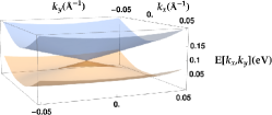
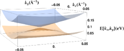
(a)(b)(c)

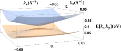
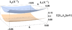
(d)(e)

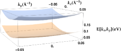
Figure 1: (Color online) The bandstructure of the two upper surface bands in the vicinity of the $\overline{X}$ point as a function of $(k_{x},k_{y})$ in the presence of a Zeeman spin-splitting of magnitude $M$, of different strengths; (a) $M=0.0$, (b) $M=0.005$, (c) $M=0.01$, (d) $M=0.05$, (e) $M=0.1$ (in eV). Note that a gap is introduced at the $\overline{X}$ point as $M$ is turned on, and with increasing values of $M$, this gap increases, and the curvature of the lower band gradually changes sign. A change in the curvature can also affect the nature of the impurity-induced bound states realized in the chiral $p-$wave superconducting state. In the paper, we work in the regime $M<m$, where the mass term $m=0.07$ eV determines the value of the energy at the $\overline{X}$ point measured with respect to the pair of Dirac points.

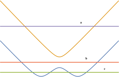
Figure 2: (Color online) Schematic illustration of the bandstructure in the vicinity of the $\overline{X}$ point, and three different doping regimes that can either result in qualitatively different electronic instabilities on the (001) surface of Pb_1-xSn_xTe (i.e. either conventional $s-$wave or chiral $p-$wave order), or lead to a difference in the nature of impurity-induced bound states realized in a chiral $p-$wave superconducting state. In (a), the Fermi level intersects two of the surface bands, which are time-reversed counterparts. In this case, interband pairing of electrons gives rise to $s-$wave superconductivity, and no Shiba-like states exist for potential defects on the surface. In (b) and (c), the pairing of the surface electrons is of the chiral $p-$wave type. We show in the paper that only the latter case, (c), when the Fermi level intersects the lower surface conduction band, Shiba-like subgap states can be unambiguously attributed to the presence of topological superconductivity.

In our analysis of impurity-induced bound states in the chiral $p-$wave superconducting state, we will work with the following Bogoliubov-de Gennes (BdG) Hamiltonian:

$$H_{0}(k)=\left(\begin{array}[]{cc}\epsilon_{k_{x},k_{y}}-\mu&\Delta(k_{x}-ik_{y})\\ \Delta(k_{x}+ik_{y})&-\epsilon_{k_{x},k_{y}}+\mu\end{array}\right),$$ (4)

where $\epsilon_{k_{x},k_{y}}$ refers to the noninteracting dispersion in Eq. 3 and $\mu$ refers to the chemical potential. This Hamiltonian acts in the Nambu space $(c_{k},c_{-k}^{\dagger})$ where $c_{k}$ are the effectively spinless fermions in the lower energy surface band, and $\Delta_{k}\equiv<c_{k}c_{-k}>=\Delta(k_{x}-ik_{y})$ is the superconducting order parameter. In the absence of $\Delta$, Eq. 4 would correspond to two copies of the Hamiltonian of a nonrelativistic particle whose energies are reckoned from an arbitrary value $\mu$. This situation is explained in more detail in Sec. III below.

Substituting the expression for $\epsilon_{k_{x}k_{y}}$ from Eq. 3 above, the spectrum corresponding to the Nambu Hamiltonian in Eq. 4 is given by $E=\pm\sqrt{(Ak^{2}+\mu^{\prime})^{2}+\Delta^{2}k^{2}}$, where $k^{2}=k_{x}^{2}+k_{y}^{2}$, and $\mu^{\prime}=\mu-C$ is an effective chemical potential reckoned from the top of the band, corresponding to the energy value closest to the higher energy surface band. We introduce dimensionless quantities

$$\lambda=\frac{\Delta^{2}}{2A|\mu^{\prime}|}$$ (5)

and

$$\epsilon=\frac{E}{|\mu^{\prime}|},$$ (6)

which appear frequently in the rest of our analysis. For non-zero values of $\mu$, the spectrum of the BdG Hamiltonian is gapped if $\Delta$ is finite. We look specifically for bound states which lie within the gap.

In general, the nature of surface electronic instabilities, and their consequences for impurity-induced bound states, depend crucially upon the position of the chemical potential with respect to the surface bands. A schematic of the band structure around the $\overline{X}$ point on the (001) surface, together with various representative positions for the chemical potential is shown in Fig. 2. If the gap is sufficiently large and the Fermi level does not intersect the upper band, then (interband) $s-$wave superconductivity, which occurs in case (a) of Fig. 2, is precluded. In the rest of the paper, we shall work in this regime. For the case (b) in Fig. 2 where the chemical potential does not intersect the lower surface conduction band, the band gap is conventional, as in, say, a semiconductor, and we call it normal. For the case (c) in Fig. 2, where it intersects this band, an additional band gap opens up at the points of intersection (not depicted in Fig. 2), due to the presence of the chiral $p-$wave superconducting order. This corresponds to an inverted band gap.

In the next section, we will try to understand the origin of impurity-induced states in the regimes (b) and (c), and how they differ from each other in the presence and absence of a chiral $p-$wave order. The role played by the distinction between these regimes in identifying the chiral $p-$wave nature of the superconducting order forms a crucial part of our paper.

III impurity states in doped semiconductors

(a)(b)

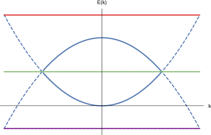
Figure 3: (Color online) Schematic illustration of the Nambu bands when (a) $\mu<0$, and the chemical potential lies in the gap (b) $\mu>0$ and the chemical potential intersects the bands, in the absence of the chiral $p-$wave order parameter $\Delta$. The bound state energies denoted by the red and purple lines lie within the gap in (a) and intersect the bands in (b). The chemical potential $\mu$ lies in the centre and is denoted by the blue line in (a) and the green line in (b). The filled and empty part of the bands are represented by thick and dashed lines respectively. Clearly, in (a) both the bands as well as the impurity states are empty.

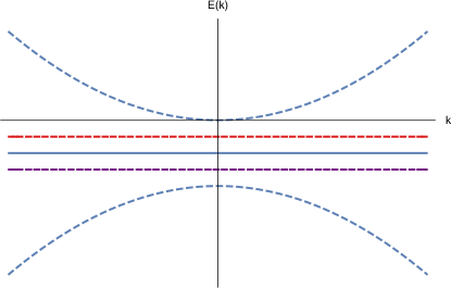
(a)(b)

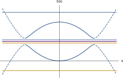
Figure 4: (Color online) Schematic illustration of the Nambu bands when (a) $\mu<0$, and the chemical potential lies in the gap (b) $\mu>0$ and the chemical potential intersects the bands, in the presence of the chiral $p-$wave order parameter $\Delta$. Clearly, an additional band gap opens in (b) due to the superconducting order. The impurity levels denoted by the red and purple lines in (a) lie within the gap, while in (b), a pair of impurity levels denoted by blue and yellow lines lie within the smaller gap while another pair intersects the two bands. The chemical potential $\mu$ lies in the centre and is denoted by the blue line in (a) and the purple line in (b). The filled and empty part of the bands are represented by thick and dashed lines respectively. In (a), both the bands as well as the impurity states are empty. These cases are discussed in detail in Sec. IV and V.

It is well-known that in one dimension, a bound state always exists for a nonrelativistic particle in the presence of an attractive Delta-function potential. Consider a single impurity in a semiconductor, and writing down the Schrodinger equation in momentum space, we have

$$(\epsilon_{k}-\mu)\psi_{k}+\int dk^{\prime}V_{k,k^{\prime}}\psi_{k^{\prime}}=E\psi_{k}$$ (7)

where $V_{k,k^{\prime}}=V_{0}$ and $\mu$ denotes the chemical potential. Using

$$\psi_{k}=\frac{-V_{0}\int dk^{\prime}\psi_{k^{\prime}}}{(\epsilon_{k}-\mu-E)}$$

and integrating both sides over the momentum $k$, we obtain the following condition on the defect potential strength $V_{0}$ for realizing impurity-induced bound states

$$V_{0}=\frac{-1}{\int\frac{dk}{(\epsilon_{k}-\mu-E)}}$$

which always gives rise to a solution, provided the integrand does not have any real poles. When such impurity bound states are present, they appear at an energy value proportional to $\sqrt{V_{0}}$ below the bottom of the conduction band and move further downwards as $V_{0}$ increases. If $\epsilon_{k}$ is the valence band of a semiconductor, then the $V_{0}$ must be positive, and the bound states appear above the top of the valence band. The existence of the impurity band is independent of the chemical potential $\mu$, but the chemical potential determines whether the impurity band is occupied or not.

Now, the same problem can be reexpressed in the Nambu representation by introducing another copy of the problem which is related to the first one by a particle-hole transformation. In the Nambu representation, the impurity bound states appear exactly as discussed above, except that since there are now two copies, for each positive impurity level, there is a corresponding negative one with the same magnitude. Consider the example of an impurity bound state arising from donor dopants in a semiconductor, and $\epsilon_{k}>0$ corresponds to the conduction band. The chemical potential is the reference energy from which all energies are measured, and in this case, the negative value of $\mu$ implies that the chemical potential does not intersect the bands, and both the bands are empty. This is illustrated in Fig. 3(a) above. On the other hand, when $\mu>0$, the bands as well as the impurity levels cross the Fermi level, and become occupied, resulting in a new situation depicted in Figs. 3(b). This is merely an artefact of the chemical potential changing sign and the levels that have crossed are those whose nature has changed from being empty to being occupied.

The situation changes dramatically in the presence of a chiral $p-$wave superconducting order. If the chemical potential $\mu<0$, the impurity levels remain empty but the bands shift in magnitude, as shown in Fig.4(a). Here, we continue to obtain subgap states and the impurity levels are indistinguishable from those in semiconductors. However, when $\mu>0$, the presence of superconductivity introduces a gap at the points where the two dispersing bands intersected, as shown in the Fig. 4(b). In this regime, the impurity levels which were formerly present only near the extrema of the upper and lower Nambu bands abruptly collapse to take values within the gap, and therefore, we now obtain subgap states.

Thus, in the presence of a chiral $p-$wave order, if $\mu<0$, one continues to obtain subgap states which are indistinguishable from impurity states in semiconductors, while if $\mu>0$, new subgap states appear due to the superconducting order in the system. In the rest of the paper, we refer to the former regime of parameters as the normal gap regime and the latter as the inverted gap regime.

IV conditions for subgap bound states with $\delta-$potential defects

We now derive the general condition for realizing subgap bound states localized in one or more directions, associated with point or linear defects on the surface of the TCI. We model such defects by a multidimensional Dirac delta-function $V(x_{i})=V_{0}\prod_{i}\delta(x_{i})$, where $i$ refers to the dimension, and $V_{0}$ represents the strength of the defect potential. The delta-function approximation for the potential defects is justified, provided that the defect potential is sufficiently smooth on the scale of the lattice constant (to avoid scattering processes between the $\overline{X_{1}}$ and $\overline{X_{2}}$ points) but nevertheless, short-ranged compared to the wavelength of the electrons.

The Schr$\ddot{\mathrm{o}}$dinger equation in momentum space, in the presence of the defect potential is given by

$$H_{0}(k)\psi_{k}+\int(d^{d}k^{\prime})V_{k,k^{\prime}}\psi_{k^{\prime}}=E\psi_{k},$$ (8)

where $H_{0}(k)$ is defined in Eq. 4 above, $E$ refers to the value of the bound state energy, and $V_{k,k^{\prime}}=V_{0}\sigma_{z}$ for the case of a point defect, and $2\pi V_{0}\delta(k_{y}-k_{y}^{\prime})\sigma_{z}$ for a linear defect along the $y-$direction. In the latter case, the integration over $k_{y}^{\prime}$ gets rid of the Delta function, leading to an equation which is diagonal in $k_{y}$ but mixes the $k_{x}$ components.

Inverting Eq. 8, we have

$$\psi_{k}=-(H_{0}(k)-EI)^{-1}V_{0}\sigma_{z}\int(d^{d}k^{\prime})\psi_{k^{\prime}},$$ (9)

where it is understood in Eq. 9 above and also in the analysis that follows that the integration runs only over $k_{x}$ for a linear defect along the $y-$direction. Next, we integrate both sides over $k$, cancel the common term $\int(d^{d}k)\psi_{k}$ on both sides and arrive at the following condition:

$$\mathrm{Det}[-\int(d^{d}k)(H_{0}(k)-EI)^{-1}V_{0}\sigma_{z}-I]=0,$$ (10)

for the bound state. Here the integration over each component of $k$ ranges from $-\infty$ to $\infty$. Note that when $\int(d^{d}k)\psi_{k}=0$, the wavefunction vanishes at the origin, and the above condition is no longer applicable, since we cannot cancel the common terms. This is, for example, true for topologically non-trivial zero-energy Majorana bound states in linear defects, for which the real-space wavefunction acquires its peak values at the physical ends of the defect and decays into the interior. When the defect being considered is infinitely long in one of the directions, the ends not being a part of the system, one cannot mathematically realize Majorana bound states within this approach. Here we have explicitly excluded such states from consideration.

Using the expression for $H_{0}(k)$ in Eq. 4, the condition in Eq. 10 translates to

$$\mathrm{Det}\left(\begin{array}[]{cc}-V_{0}I_{1}(0,0,E)-1&V_{0}I_{3}(0,0,E)\\ -V_{0}I_{4}(0,0,E)&-V_{0}I_{2}(0,0,E)-1\end{array}\right)=0,$$ (11)

where we define

$$I_{1,2}(x,y,E)=\int_{-\infty}^{\infty}(dk_{x})(dk_{y})\exp[ik_{x}x]\exp[ik_{y}y]\frac{\epsilon_{k_{x},k_{y}}-\mu\pm E}{(\epsilon_{k_{x},k_{y}}-\mu)^{2}-E^{2}+\Delta^{2}(k_{x}^{2}+k_{y}^{2})},$$ (12)

and

$$I_{3,4}(x,y,E)=\int_{-\infty}^{\infty}(dk_{x})(dk_{y})\exp[ik_{x}x]\exp[ik_{y}y]\frac{\Delta(k_{x}\mp ik_{y})}{(\epsilon_{k_{x},k_{y}}-\mu)^{2}-E^{2}+\Delta^{2}(k_{x}^{2}+k_{y}^{2})}.$$ (13)

Let us consider first the case of point defects. From Eq. 11, we obtain the following condition for the strength of the defect potential $V_{0}$ that gives a bound state at energy $E$:

$$(V_{0}I_{1}(0,0,E)+1)(V_{0}I_{2}(0,0,E)+1)=0.$$ (14)

From Eq. 14, it is evident that for a given value of $V_{0}$, we have a pair of bound states with energies $\pm E$, which is a reflection of particle-hole symmetry of the BdG Hamiltonian. Conversely, for every value of the bound state energy there exist two possible values for the strength of the defect potential, $V_{0}$, which do not in general have the same magnitude, for which one may realize such a state.

For a line defect of infinite length along, say, the $y-$direction, the defect potential may be written as $V(x)=V_{0}\delta(x)$, such that the translational symmetry is broken only along the $x-$direction. In this case, we obtain, from Eq. 11, the following condition for realizing a subgap bound state with an energy $E$, where $k_{y}$ is conserved and takes real values.

$$(V_{0}I_{1}(0,0,E)+1)(V_{0}I_{2}(0,0,E)+1) +V_{0}^{2}I_{3}(0,0,E)I_{4}(0,0,E)=0.$$ (15)

The relation between $V_{0}$ and $E$ is

$$V_{0}(E)=\frac{-(I_{1}+I_{2})\pm\sqrt{(I_{1}-I_{2})^{2}-4I_{3}I_{4}}}{2(I_{1}I_{2}+I_{3}I_{4})}.$$ (16)

Since $V_{0}$ is real, the discriminant must be positive, resulting in a condition which relates the allowed values of the bound state energy to the quantum number $k_{y}$ i.e. $\mathrm{min}(E_{g}^{2},(\mu^{\prime})^{2})$$\geq E^{2}\geq\Delta^{2}k_{y}^{2}$. The lowest energy bound states clearly correspond to the case where $k_{y}=0$. This leads to the conditions $1+I_{1}V_{0}=0$, or $1+I_{2}V_{0}=0$.

From Eq. 9, we can also obtain expressions for the bound state wavefunctions. Taking an inverse Fourier transform on both sides, we obtain the following expression for the wavefunction in real space:

$$\psi(x,y) =\left(\begin{array}[]{c}a(x,y)\\ b(x,y)\end{array}\right)=(-V_{0})\left(\begin{array}[]{c}I_{1}(x,y,E)a_{0}-I_{3}(x,y,E)b_{0}\\ I_{2}(x,y,E)b_{0}+I_{4}(x,y,E)a_{0}\end{array}\right),$$ (21)

where $\psi_{0}=\left(\begin{array}[]{c}a_{0}\\ b_{0}\end{array}\right)$ is the real-space wavefunction at the origin, i.e. $\psi(0,0)$, and $I_{1,2}(x,y,E)$ and $I_{3,4}(x,y,E)$ are as defined in Eqs. 12 and 13. The normalization condition is

$$\int dx\int dy(|a(x,y)|^{2}+|b(x,y)|^{2})=1.$$ (22)

For the case of a point defect, we find that, for any non-zero value of the bound state energy $E$, putting $x=y=0$ on both sides of Eq. 21 above results in the elimination of one of the components $a_{0}$ or $b_{0}$ when the condition in Eq.14 is satisfied. For $E=0$, however, it simply gives rise to a consistency condition without yielding any new information about the components at the origin, and the only constraint on the constants $a_{0}$ and $b_{0}$ is then the normalization condition in Eq. 22. This is a manifestation of an internal SU(2) rotational symmetry (in particle-hole space), which makes the zero energy state centred at the origin useful as a possible quantum qubit. A similar condition is also obtained for a linear defect, but in the specific case where $k_{y}=0$. Since there are arbitrarily close bound states parametrized by nonzero $k_{y}$, the zero energy state is not useful as a qubit for the case of linear defects.

IV.1 Absence of subgap states for $s-$wave superconductivity:

As discussed in Sec.II, pairing between time-reversed surface bands can lead to $s-$wave superconductivity on the (001) surface. We shall now show that subgap bound states in isolated potential defects can no longer be realized for a conventional $s-$wave superconducting order in this system.

The $s-$wave order parameter can be written as $\Delta$, which is a momentum-independent constant. Following Eq. 11 , the condition for realizing subgap bound states with an energy $E$ in the presence of surface potential defects in this case is given by

$$\mathrm{Det}\left(\begin{array}[]{cc}-V_{0}\int(dk_{x})(dk_{y})\frac{\epsilon_{k_{x},k_{y}}-\mu+E}{(\epsilon_{k_{x},k_{y}}-\mu)^{2}-E^{2}+\Delta^{2}}-1&V_{0}\int(dk_{x})(dk_{y})\frac{\Delta}{(\epsilon_{k_{x},k_{y}}-\mu)^{2}-E^{2}+\Delta^{2}}\\ -V_{0}\int(dk_{x})(dk_{y})\frac{\Delta}{(\epsilon_{k_{x},k_{y}}-\mu)^{2}-E^{2}+\Delta^{2}}&-V_{0}\int(dk_{x})(dk_{y})\frac{\epsilon_{k_{x},k_{y}}-\mu-E}{(\epsilon_{k_{x},k_{y}}-\mu)^{2}-E^{2}+\Delta^{2}}-1\end{array}\right)=0.$$ (23)

From Eq. 23, the possible values of $V_{0}(E)$ are given by

$$V_{0}=\frac{-(a+b)\pm\sqrt{(a-b)^{2}-4c^{2}}}{2(ab+c^{2})},$$

where $a,b=\int(dk_{x})(dk_{y})(\epsilon_{k_{x},k_{y}}-\mu\pm E)/((\epsilon_{k_{x},k_{y}}-\mu)^{2}-E^{2}+\Delta^{2})$ and $c=\int(dk_{x})(dk_{y})(\Delta/((\epsilon_{k_{x},k_{y}}-\mu)^{2}-E^{2}+\Delta^{2}))$. Clearly, real values of $V_{0}$ require the discriminant to be positive, i.e. $|E|\geq\Delta$, and thus, no subgap bound states are possible. The above arguments also hold true for a mixed $s+p-$wave superconducting order.

V bound state spectra and wavefunctions

We now use the results obtained in Sec. IV above in the context of subgap impurity bound states in Pb_1-xSn_xTe. In the analysis that follows, we shall distinguish between the situations where the chemical potential lies within the conventional or normal band gap between the pair of surface bands, and those where it intersects the lower surface conduction band, giving rise to an inverted band gap at small momenta. We shall find that the subgap states that arise in the inverted band gap situation crucially depend on the existence of the chiral $p-$wave order. On the other hand, in the normal band gap situation, the impurity bound states are not qualitatively affected in the limit where the chiral $p-$wave order is absent. Note that in what follows, we will be working with the valence band, as that is the physical situation prevailing in our system, and without loss of generality, the considerations discussed in Sec. III are carried through.

V.1 Point defects:

Let us first consider the case of a point defect. In plane polar coordinates, Eq. 14, relating the impurity strength to the bound state energy $E$, takes the form

$$\frac{1}{V_{0}}=\frac{1}{4\pi}\int_{0}^{\Lambda^{2}}d\upsilon\frac{(A\upsilon+\mu^{\prime})\mp E}{(A\upsilon+\mu^{\prime})^{2}-E^{2}+\Delta^{2}\upsilon},$$ (24)

where $\upsilon=k^{2}$ and $\mu^{\prime}\equiv\mu-C$, and $\Lambda$ is the large momentum cutoff, physically corresponding to the inverse of the width of the potential well, which is approximated to be a Delta-function potential in our treatment. We now examine Eq. 24 respectively in the normal and inverted band gap regimes.

V.1.1 Conditions for bound states in different parameter regimes

(a) Normal band gap: $\mu^{\prime}>0$

When the chemical potential $\mu>C$ (or $\mu^{\prime}>0$), the condition for subgap bound states in Eq. 24 above evaluates to

$$\frac{1}{V_{0}} \approx\frac{1}{2A\sqrt{\left(\lambda+1\right)^{2}-\left(1-\epsilon^{2}\right)}}\left[\left(\lambda\pm\epsilon\right)\ln\left|\frac{\lambda+1-\sqrt{(\lambda+1)^{2}-(1-\epsilon^{2})}}{\lambda+1+\sqrt{(\lambda+1)^{2}-(1-\epsilon^{2})}}\right|\right.$$

$$\left.+\sqrt{\left(\lambda+1\right)^{2}-\left(1-\epsilon^{2}\right)}\left(\ln|\frac{A^{2}\Lambda^{4}}{|\mu^{\prime}|^{2}(1-\epsilon^{2})}|\right)\right].$$ (25)

For any value of the bound-state energy $|E|<\mu^{\prime}$, we find that $(\lambda\pm\epsilon)<\sqrt{(\lambda+1)^{2}-(1-\epsilon^{2})}$, implying that $V_{0}$, is always a positive quantity. Physically, this corresponds to impurity (hole) states near the valence band of a semiconductor, and in this regime, one always obtains subgap states, even when $\Delta$ is turned off. The impurity levels here lie in the manner shown in Fig. 4(a).

(b) Inverted band gap: $\mu^{\prime}<0$

Here, the chemical potential $\mu<C$, or $\mu^{\prime}<0$, and this corresponds to the inverted band gap situation, which corresponds to the expression in Eq. 25 above, with $\lambda\rightarrow-\lambda$. In this case, a gap opens either at $k=0$ or at the points of intersection of the two Nambu bands (see Fig. 4(b)). If, in this regime, $\Delta$ is turned off, this gap will close and the impurity levels will be pushed away to the positions originally predicted for impurity states in a semiconductor (see Fig. 3(b)).

V.1.2 Quasi-localized bound state wavefunctions for point defects

Let us now calculate the expressions for the bound state wavefunctions for the case of a point defect. From Eq. 21, it can be seen that the spatial dependence of the bound-state wavefunctions is determined by the integrals $I_{1,2}(x,y,E)$ and $I_{3,4}(x,y,E)$, defined in Eqs. 12 and 13 respectively. In plane polar coordinates, these equations assume the form

$$I_{1}(r)=-\frac{1}{(2\pi)^{2}}\int dkd\phi\,k\exp[ikr\cos[\theta-\phi]]\frac{(Ak^{2}+\mu^{\prime})\mp E}{(Ak^{2}+\mu^{\prime})^{2}-E^{2}+\Delta^{2}k^{2}}$$ (26)

and

$$I_{2}(r,\theta)=\frac{1}{(2\pi)^{2}}\exp[i\theta]\int dkd\phi\,k\exp[ikr\cos[\phi]]\exp[i\phi]\frac{\Delta k}{(Ak^{2}+\mu^{\prime})^{2}-E^{2}+\Delta^{2}k^{2}}$$ (27)

where $\mu^{\prime}\equiv\mu-C$, $k=\sqrt{k_{x}^{2}+k_{y}^{2}}$, and $\phi=\arctan[y/x]$. We illustrate the specific case of $E=0$ where analytical expressions for the wavefunctions can be obtained in terms of elementary functions, and expect qualitatively similar results for other bound-state energies with $E\neq 0$. We once again consider regimes with a normal and an inverted band gap.

(a) Normal band gap: $\mu^{\prime}>0$

Using the well-known result $\int d\phi\exp[ikr\cos[\theta-\phi]=2\pi J_{0}(kr)$, the expression of $I_{1}(r)$ from Eq. 26 is as follows:

$$I_{1}(r) =\frac{1}{4\pi}\int dkkJ_{0}(kr)\frac{2}{A(\alpha+\beta)}\left(\frac{\alpha}{k^{2}+\alpha^{2}}+\frac{\beta}{k^{2}+\beta^{2}}\right)$$

$$=-\frac{1}{2\pi A(\alpha+\beta)}\left(\alpha K_{0}\left(\alpha r\right)+\beta K_{0}\left(\beta r\right)\right),$$ (28)

where $\alpha,\beta=\sqrt{\mu^{\prime}/A}((\sqrt{(\lambda+2}\pm\sqrt{\lambda})/\sqrt{2})$.

Thus, we find that $I_{1}(r)$ is an exponentially decaying function of at large distances $r$ from the position of the defect. Note that when $\Delta=0$, i.e. $\lambda=0$, $\alpha$ and $\beta$ are real, giving rise to exponentially decaying states.

Similarly, using the result $\int d\phi\exp[ikr\cos[\theta-\phi]]\exp[i\phi]=i2\pi J_{1}(kr)$, we may simplify the expression for $I_{2}$ given in Eq. 27 as

$$I_{2}(r,\theta) =\frac{-i\exp[i\theta]}{2\pi A(\alpha+\beta)}\int\frac{dx}{r}J_{1}(x)\left(\frac{\beta^{2}r^{2}}{x^{2}+\beta^{2}r^{2}}-\frac{\alpha^{2}r^{2}}{x^{2}+\alpha^{2}r^{2}}\right)$$

$$\approx\frac{-i\exp[i\theta]}{2\pi A(\alpha+\beta)}\frac{1}{r^{2}}\left(\frac{1}{\alpha}-\frac{1}{\beta}\right),$$ (29)

where $kr\equiv x$, $\alpha,\beta=\sqrt{\mu^{\prime}/A}((\sqrt{\lambda+2}\pm\sqrt{\lambda})/\sqrt{2})$, and in the second line we have used the relation

$$\int_{0}^{\infty}\frac{J_{\nu}(x)}{x^{2}+a^{2}}dx=\frac{\pi\left(\mathbf{J_{\nu}}(a)-J_{\nu}(a)\right)}{a\sin[\nu\pi]},$$ (30)

and the asymptotic expansion for the Anger function $\mathbf{J_{\nu}}(a)$,Gradshteyn and Ryzhik (2007)

$$\left.\frac{\mathbf{\pi(J_{\nu}}(a)-J_{\nu}(a))}{a\sin[\nu\pi]}\right|_{\nu\rightarrow 1}=\frac{1}{a^{2}}[1-\sum_{n=0}^{p-1}(-1)^{n}2^{2n+1}\Gamma\left(n+\frac{3}{2}\right)\frac{\Gamma\left(n+\frac{1}{2}\right)}{\pi}a^{-2n-1}+...].$$ (31)

We therefore find that the function $I_{2}(r,\theta)$ decays as an inverse square power law at large distances, and not exponentially. This also determines the overall asymptotic behavior of the bound state wavefunction, which tends to be quasi-localized at large distances from the defect. We find that the chiral $p-$wave symmetry of the superconducting order is directly responsible for the power-law decaying asymptotic behavior. Moreover, when $\lambda=0$ (i.e. in the absence of superconductivity) the power-law decaying component vanishes and one is then left with an exponentially decaying contribution, similar to impurity bound states in a semiconductor.

(b) Inverted band gap: $\mu^{\prime}<0$

Here, we consider a situation where $\mu<C$, or $\mu^{\prime}<0$, and repeat the analysis of the previous section by replacing $\mu^{\prime}$ by $-|\mu^{\prime}|$ in Eqs. 26 and 27.

For $\lambda\geq 2$, we then have,

$$I_{1}(r) =\frac{1}{2\pi}\int dk\,kJ_{0}(kr)\frac{1}{A(\alpha-\beta)}\left(\frac{2\alpha}{k^{2}+\alpha^{2}}-\frac{2\beta}{k^{2}+\beta^{2}}\right)$$

$$=\frac{1}{2\pi A(\beta-\alpha)}\left(\alpha K_{0}(\alpha r)-\beta K_{0}(\beta r)\right),$$

where now $\alpha,\beta=\sqrt{\mu^{\prime}/A}((\sqrt{\lambda}\pm\sqrt{\lambda-2})/\sqrt{2})$. Similarly, from Eq. 27, we write the expression for $I_{2}(r,\theta)$ as

$$I_{2}(r,\theta) =\frac{i}{2\pi}\exp[i\theta]\int dk\,J_{1}(kr)\frac{1}{(A)}\frac{1}{(\beta-\alpha))}\left(\frac{\beta^{2}}{k^{2}+\beta^{2}}-\frac{\alpha^{2}}{k^{2}+\alpha^{2}}\right)$$

$$\approx\frac{i\exp[i\theta]}{2\pi A(\beta-\alpha)}\left(\frac{1}{r^{2}}\left(\frac{1}{\alpha}-\frac{1}{\beta}\right)\right)$$

where $\alpha,\beta=\sqrt{\mu^{\prime}/A}((\sqrt{\lambda}\pm\sqrt{\lambda-2})/\sqrt{2})$, following steps similar to the previous case, where $\mu^{\prime}>0$. The results obtained are identical for $\lambda<2$, but with $\alpha,\beta=\sqrt{|\mu^{\prime}|/A}((\sqrt{\lambda}\mp i(\sqrt{2-\lambda})/\sqrt{2}$). While the inverse-square decay of the wavefunction is common to both the normal and inverted band gap situations, the coefficient of the inverse square term happens to be independent of the value of $\Delta$ in the inverted band gap case. Please refer to Appendix-B for a detailed derivation of the asymptotic forms of the bound state wavefunctions.

In contrast to a chiral superconductor, a nodal superconductor gives a qualitatively different wavefunction for the impurity bound state. For instance, when the superconducting order parameter $\Delta_{k}=\Delta k\cos[\phi]$, we have

$$I_{2}(r,\theta)=\frac{\cos[\theta]}{(2\pi)}\int dk\,k\frac{\Delta k}{(Ak^{2}+\mu^{\prime})^{2}+\Delta^{2}k^{2}}iJ_{1}(kr).$$

Similarly, for $\Delta_{k}=\Delta k\sin[\phi]$,

$$I_{2}(r,\theta)=\frac{\sin[\theta]}{(2\pi)}\int dk\,k\frac{\Delta k}{(Ak^{2}+\mu^{\prime})^{2}+\Delta^{2}k^{2}}iJ_{1}(kr).$$

Thus, unlike a chiral $p-$wave superconductor, the above types of superconducting order feature nodal lines in the bound-state wavefunction, at large distances from the position of the defect. One could use STM imaging of the bound-state wavefunctions as a means to distinguish between nodal and chiral $p-$wave order on the surface.

Incidentally, our results qualitatively differ from the bound state wavefunctions proposed earlier in this context using a variational ansatz Maki and Haas (2000); Haas and Maki (2000). The asymptotic behavior of the bound state wavefunctions in a point defect has also been calculated in a recent work, Kaladzhyan et al. (2016a) and found to be exponentially decaying. This treatment, however, assumes a constant density of states at the Fermi surface to evaluate integrals analogous to those in Eqs.26 and 27. This is a questionable assumption, given that the large-distance behavior is governed by small momenta, where the density of states linearly goes to zero with momentum. In Appendix-C, we show the derivation of the asymptotic form of the bound state wavefunction for a linear dispersion, similar to the one considered (close to the Fermi surface) in Ref. Kaladzhyan et al., 2016a, without any assumptions, and once again obtain a power law decay at large distances.

V.2 Line defects

Here we study the nature of bound states for long linear defects. In this case, we write the defect potential as $V(x,y)=V_{0}\delta(x\cos[\alpha]+y\sin[\alpha])$, and consider the special case of $\alpha=0$, i.e. $V(x)=V_{0}\delta(x)$. Once again, we study the two regimes with a normal and an inverted band gap, respectively.

(a) Normal band gap: $\mu^{\prime}>0$

Following Eq. 15, the relation between $V_{0}$ and the bound state energy $E$ (for $k_{y}=0$) is given by

$$\frac{1}{V_{0}}=\frac{1}{(2\pi)}\int_{0}^{\infty}\frac{dy}{2\sqrt{y}}\frac{(-Ay-\mu^{\prime}\pm E)}{A^{2}(y+a)(y+b)},$$ (32)

where $\mu^{\prime}\equiv\mu-C$, $y=k_{x}^{2}$ and $a,b=(\mu^{\prime}/A)((\lambda+1\mp\sqrt{((\lambda+1)^{2}-(1-\epsilon^{2})})$. Evaluating the integral in Eq. 32, we arrive at

$$V_{0,\pm}=\frac{4A(\sqrt{a}+\sqrt{b})}{(1+\sqrt{(1\mp\epsilon)/(1\pm\epsilon)})},$$ (33)

with $\sqrt{ab}=|\mu^{\prime}|\sqrt{1-\epsilon^{2}}/A$. The variation of $V_{0}$ as a function of the bound state energy $E$ is shown in Fig. 5. Here we find a trivial crossing of the energy level with the chemical potential as $V_{0}$ is tuned, which does not depend on the presence of superconductivity. A similar crossing has also been observed in Ref. Sau and Demler, 2013, where it has been used to characterize the topological superconducting phase. We emphasize here that the crossing that we observe is an artefact of the Nambu representation, and would appear even in the absence of superconductivity. The origin of the zero-energy crossings has also been discussed in Sec. III above.

The subgap bound states in this case form a part of a continuum of states parametrized by different values of $k_{y}$. The corresponding expression obtained by solving Eq. 15 for a finite, real value of $k_{y}$ is given by

$$V_{0,\pm}=\frac{2A(\sqrt{a}+\sqrt{b})\sqrt{1\pm\epsilon_{e}}\left(\sqrt{1\mp\epsilon_{e}}+\sqrt{1\pm\epsilon_{e}}\right)}{\left(\sqrt{1-\epsilon_{e}^{2}}+1\right)},$$

with $a,b=(\mu_{e}/A)(\lambda_{e}+1\mp\sqrt{(\lambda_{e}+1)^{2}-(1-\epsilon_{e}^{2})})$, $\mu_{e}=\mu^{\prime}+Ak_{y}^{2}$, $E_{e}^{2}=E^{2}-\Delta^{2}k_{y}^{2}$ and $\lambda_{e}=\Delta^{2}/(2A|\mu_{e}|)$. Clearly, $V_{0}$ is always positive in this case, corresponding to hole-like states near the valence band.

(b) Inverted band gap: $\mu^{\prime}<0$

When the chemical potential intersects the lower surface conduction band, we have $\mu^{\prime}<0$. Evaluating the resulting integral from Eq. 15, we obtain the relation

$$V_{0,\pm}=\frac{4A(\sqrt{a}+\sqrt{b})}{(1-\sqrt{(1\pm\epsilon)/(1\mp\epsilon)})},$$ (34)

where $a,b=(|\mu^{\prime}|/A)(\lambda-1\mp\sqrt{(\lambda-1)^{2}-(1-\epsilon^{2})})$. Clearly, in this case, the amplitude of the defect potential may change sign depending upon the value of the bound state energy $E$ under consideration, and in general, subgap bound states can be realized for both potential wells and barriers, corresponding to particle-like and hole-like states, as is also evident from Fig. 5.In the limit $V_{0}\rightarrow\infty$, we find a doubly-degenerate zero energy bound state, reminiscent of two-fold degenerate zero-energy bound states in the honeycomb Kitaev model with a missing site.Willans et al. (2011, 2010) Such a correspondence is perhaps unsurprising, given that the honeycomb Kitaev model sits on the verge of a transition to a chiral $p-$wave superconductor.You et al. (2012)

Similarly, for a finite, real value of $k_{y}$, we obtain the relation

$$V_{0,\pm}=\frac{2A(\sqrt{a}+\sqrt{b})\sqrt{1\mp\epsilon_{e}}\left(\sqrt{1\pm\epsilon_{e}}-\sqrt{1\mp\epsilon_{e}}\right)}{\left(\sqrt{1-\epsilon_{e}^{2}}-1\right)},$$

where $\mu_{e}=\mu^{\prime}-Ak_{y}^{2}$, $E_{e}^{2}=E^{2}-\Delta^{2}k_{y}^{2}$, and $a,b=(|\mu_{e}|/A)(\lambda_{e}-1\mp\sqrt{(\lambda_{e}-1)^{2}-(1-\epsilon_{e}^{2})}$) . Note that the above expression is only applicable in the regime where $\epsilon_{e}^{2}<1$.

On the other hand, for $\epsilon_{e}^{2}>1$, which can only be satisfied for $\mu^{\prime}<0$, we have the alternate expression

$$V_{0,\pm}=\frac{4A^{2}\sqrt{b}\left(b+a\right)\left(Ab+|\mu_{e}|\left(1\pm\epsilon_{e}\right)\right)}{\left(A^{2}b^{2}+2A|\mu_{e}|b+\mu_{e}^{2}\left(1-\epsilon_{e}^{2}\right)\right)},$$ (35)

where $a,b=(\mu_{e}/A)(\sqrt{(\lambda_{e}-1)^{2}-(1-\epsilon_{e}^{2})}\mp(\lambda_{e}-1))$. The RHS in Eq. 35 may change sign for bound state energies satisfying the condition $|\epsilon_{e}|>\lambda_{e}$.

Apart from the above two kinds of isolated potential defects, one can also consider situations where the surface of the topological crystalline insulator is homogeneously disordered. In Appendix-A, we have determined the optimal potential fluctuation for realizing zero-energy bound states, by adapting a Lifshitz-tail like treatment from the literature on disordered conductors. For homogeneously distributed one-dimensional defects (with translational symmetry preserved along one of the directions), we have confirmed that no zero-energy states can be realized in the topologically nontrivial situation where the chemical potential intersects the lower surface conduction band.

Figure 5: (Color online) The figure showing the variation in the strength of the defect potential $V_{0}$ required to give a subgap bound state, as a function of the magnitude of the bound state energy $E$ for a line defect. The cases considered are: (a) $\mu^{\prime}>0$ for a normal band gap (b) $\mu^{\prime}<0$ for an inverted band gap. The parameters chosen are $A=4.0$ eVÅ, $\mu^{\prime}=20$ meV and $\Delta=5$ meVÅ. We find the behavior to be qualitatively different in the two cases. In the latter case, $V_{0}\rightarrow\infty$ as $E\rightarrow 0$ and the defect potential strength $V_{0}$ can change sign, which opens up the possibility of realizing subgap bound states for both potential wells and barriers of various sizes. Here, 1 and 2, denoted by the solid and dashed curves respectively, refer to the two solutions obtained for the strength of the potential $V_{0}$. The dashed line refers to the value of the energy gap, which is given by $2|\mu^{\prime}|$ for the topologically trivial regime in (a) and $2E_{g}$ for the topologically nontrivial regime in (b). See discussion in main text for a comparison with the result in Ref. Sau and Demler, 2013.

VI conclusions

In summary, we have examined the parameter regimes where a stable chiral $p-$wave superconducting order can exist on the (001) surface of Pb_1-xSn_xTe, depending upon the position of the chemical potential and the strength of the Zeeman splitting. Within the chiral $p-$wave regime, we further identified two situations, corresponding to the normal and the inverted band gap and showed that while Shiba-like states can exist in both these regimes, only in the latter case, the subgap states can be attributed to the presence of a chiral $p-$wave superconducting order. By tuning the chemical potential in the latter regime, one can use local probes to identify the nature of the superconducting order observed on the (001) surface of Pb_1-xSn_xTe. Shiba-like states could be a more reliable probe for detecting topological superconductivity in this material, as compared to the conventional strategy of detecting zero-bias anomalies, putatively Majorana bound states. This is particularly important since it has been shown in recent studies of Pb_1-xSn_xTe that even at high temperatures, when superconductivity is absent, zero-bias anomalies sharing many features that are traditionally attributed to Majorana bound states can appear, due to the presence of stacking faults.Sessi et al. (2016); Iaia et al. (2018) The possibility of such errors arising in the interpretation of zero-bias anomalies have also been discussed in the context of other topological materials. Yam et al. (2018)

Using our exact analytical expressions, we show that the bound state wavefunctions for point defects in two dimensions decay monotonously as an inverse-square power law at large distances, without showing any Friedel-like oscillations. On the other hand, in the normal gap regime, the power-law states give way to conventional exponentially localized states upon the loss of superconducting order, which are qualitatively similar to subgap states in disordered semiconductors. As a possible application of our results, we show that for the case of point defects, the wavefunctions corresponding to the zero-energy bound states have an internal SU(2) rotational symmetry, which makes them useful as possible quantum qubits. We have found a number of points of divergence from existing results on impurity bound states in chiral superconductors. In an earlier work, Sau and Demler (2013) the crossing of the particle-like and hole-like impurity bound state solutions at zero energy was identified as a signature for topological superconductivity, and we show that this is an artefact related to the BdG structure of the Hamiltonian and would occur even when applied to a non-superconducting system such as a semiconductor. Our results for the asymptotic behavior of the bound state wavefunctions in a point defect also differ from the existing literature, where they are expected to be exponentially localized,Kaladzhyan et al. (2016a) and we trace the origin of the discrepancies with our results to the assumption of a constant density of states at the Fermi level in the earlier treatment. Interestingly, we found similarities between properties of the bound states realized on the surface of the TCI, and those associated with missing sites in the honeycomb Kitaev model,Willans et al. (2011, 2010); Dhochak et al. (2010); Das et al. (2016b) possibly arising from the fact that the latter sits on the verge of a chiral $p-$wave superconducting transition, and can indeed be made to exhibit it upon doping.You et al. (2012) These similarities will be explored further in future work.

The analytical strategy which we have introduced can be used to study bound states in defects with other symmetries. One interesting case to consider would be that of a semi-infinite line defect, modeled by a two-dimensional Delta-function potential $V(r,\phi)=\lambda\delta(\phi)$. The interesting thing here would be to look for the zero energy Majorana bound state at $r=0$, and obtain its wavefunction analytically. One can also study problems involving junctions of line defects, or regular arrays of defects. Our approach can also be applied to other types of unconventional superconductivity, such as a chiral $d-$wave order.

Appendix A Optimal potential fluctuation for homogeneously distributed defects

We consider homogeneously distributed one-dimensional defects on the surface of the TCI, such that translational symmetry is preserved along one of the directions. We first discuss the approach used for determining the optimal potential fluctuation, in the case of a spatially uncorrelated potential disorder with a Gaussian distribution. We follow a statistical approach (see, for example, Ref. Altland and Simons, ), assuming that the disorder may be represented by a random potential $U(x)$ with a short-range Gaussian distribution, whose statistical properties are described by a probability measure $P[U]$, i.e.,

$$P[U]=\exp\left[-\frac{1}{2\gamma^{2}}\int d^{d}xd^{d}x^{\prime}\,U(x)K^{-1}(x-x^{\prime})U(x^{\prime})\right],$$ (36)

where the spatial correlation function for the disorder is given by $<U(x)U(x^{\prime})>=\gamma^{2}K(x-x^{\prime})\equiv\gamma^{2}\delta(x-x^{\prime})$.

In order to obtain the most probable potential distribution, at a fixed value for the bound-state energy $E$, we need to minimize the following functional over $U(x)$

$$F[U(x),\psi(x)]=\int d\Omega\,\,U^{2}(x)-\eta\int d\Omega\,\,\psi^{\dagger}(x)(H-E)\psi(x),$$

where $H=A\sigma_{3}\nabla^{2}-i\Delta\sigma_{1}\nabla-\mu^{\prime}\sigma_{3}+U(x)\sigma_{3}$ for a parabolic dispersion, which gives us the relation $U(x)=\frac{\eta}{2}\psi^{\dagger}(x)\sigma_{3}\psi(x)$. Using this condition to eliminate $\eta$, we now self-consistently solve the Schr$\mathrm{\ddot{o}}$dinger equation in the presence of chiral $p-$wave superconductivity on the surface, and calculate the optimal potential distribution $U(x)$.

In the presence of a chiral $p-$wave superconducting order on the surface, the Schr$\ddot{\mathrm{o}}$dinger equation may be written as follows:

$$A\sigma_{3}\frac{d^{2}\psi}{dx^{2}}-i\Delta\sigma_{1}\frac{d\psi}{dx}-\mu^{\prime}\sigma_{3}\psi+V_{0}(\psi^{\dagger}\sigma_{3}\psi)\sigma_{3}\psi=0,$$ (37)

where $V_{0}=\eta/2$, and we specifically consider a zero-energy bound state, such that $k_{y}=0$. The process of solving Eq. 37 is enormously simpified by performing a gauge transformation, given by $\psi=\exp[iW(x-x_{0})]\Phi$. Note that such a transformation becomes necessary only due to the presence of the chiral $p-$wave superconducting order. The same transformation works in the absence of $p-$wave superconductivity, with $W=0$.

The matrix $W$ may be chosen such that the coefficient of $d\Phi/dx$ vanishes, i.e. $2A\sigma_{3}(W)=\mathbf{\triangle}\sigma_{1}$ and $W=(1/(2A))\Delta i\sigma_{2}$. Substituting this back into Eq. 37, we find

$$A\sigma_{3}W^{2}\exp[iW(x-x_{0})]\Phi+A\sigma_{3}\exp[iW(x-x_{0})]\frac{d^{2}\Phi}{dx^{2}}-\mu^{\prime}\sigma_{3}\exp[iW(x-x_{0})]\Phi$$

$$+V_{0}(\Phi^{\dagger}\exp[-iW^{\dagger}(x-x_{0})]\sigma_{3}\exp[iW(x-x_{0})]\Phi)\sigma_{3}\exp[iW(x-x_{0})]\Phi=0.$$ (38)

The gauge-transformation leaves $\sigma_{3}$ invariant, i.e.$\exp[-iW^{\dagger}(x-x_{0})]\sigma_{3}\exp[iW(x-x_{0})]=\sigma_{3}$.

Multiplying Eq. 38 by $\exp[-iW^{\dagger}(x-x_{0})]$ throughout and replacing $W^{2}$ by $(-\Delta^{2}/(4A^{2}))I$, we arrive at the condition

$$-\frac{\Delta^{2}}{4A}\sigma_{3}\Phi+A\sigma_{3}\frac{d^{2}\Phi}{dx^{2}}-\mu^{\prime}\sigma_{3}\Phi+V_{0}(\Phi^{\dagger}\sigma_{3}\Phi)\sigma_{3}\Phi=0$$ (39)

The Hermitian conjugate of the above equation is given by

$$-\frac{\Delta^{2}}{4A}\Phi^{\dagger}\sigma_{3}+A\frac{d^{2}\Phi^{\dagger}}{dx^{2}}\sigma_{3}-\mu^{\prime}\Phi^{\dagger}\sigma_{3}+V_{0}(\Phi^{\dagger}\sigma_{3}\Phi^{\dagger})\sigma_{3}\Phi=0.$$ (40)

We multiply Eq. 39 on the left by $d\Phi^{\dagger}/dx$ and Eq. 40 on the right by $d\Phi/dx$, and adding the resulting set of equations, arrive at the expression

$$A\frac{d\Phi^{\dagger}}{dx}\sigma_{3}\frac{d\Phi}{dx}=\mu^{\prime}\left(\mp\frac{\lambda}{2}+1\right)(\Phi^{\dagger}\sigma_{3}\Phi)-\frac{V_{0}}{2}(\Phi^{\dagger}\sigma_{3}\Phi)^{2}$$ (41)

where $\lambda$ is as defined in Eq. 5 and the signs $\mp$ correspond to $\mu^{\prime}<0$ and $\mu^{\prime}>0$, respectively. For simplicity, let us consider a solution of the form $\Phi=\left(\begin{array}[]{c}a\\ b\end{array}\right)$, where $a(x)$ and $b(x)$ are assumed to be real functions. Then, Eq. 41 then gives us the condition

$$A(\left(\frac{da}{dx}\right)^{2}-\left(\frac{db}{dx}\right)^{2})=\mu^{\prime}\left(\frac{\mp\lambda}{2}+1\right)(a^{2}-b^{2})-\frac{V_{0}}{2}(a^{2}-b^{2})^{2}$$

We find that one may obtain solutions for the special cases where $a=0$ or $b=0$, i.e. $\Phi=\left(\begin{array}[]{c}a\\ 0\end{array}\right)$ or $\Phi=\left(\begin{array}[]{c}0\\ b\end{array}\right)$. This leads to the following set of equations

$$A\left(\frac{da}{dx}\right)^{2}=\mu^{\prime}\left(\mp\frac{\lambda}{2}+1\right)a^{2}-\frac{V_{0}}{2}a^{4}$$ (42)

$$A\left(\frac{db}{dx}\right)^{2}=\mu^{\prime}\left(\mp\frac{\lambda}{2}+1\right)b^{2}+\frac{V_{0}}{2}b^{4}.$$ (43)

It can be seen from Eq. 42 and 43 that in the topologically nontrivial regime with $\mu^{\prime}<0$, where $\lambda\leq 2$, the above equations cannot give rise to zero-energy bound state solutions, for any value of $V_{0}$.

Now, simplifying Eq. 42, we have

$$\frac{1}{\sqrt{C_{1}}}\frac{da}{dx}=\xi\frac{a}{\sqrt{C_{1}}}\sqrt{1-\frac{a^{2}}{C_{1}}},$$

where $C_{1}=2\mu^{\prime}(\mp(\lambda/2)+1)/V_{0}$. This can be rewritten as

$$\frac{d\alpha}{\alpha\sqrt{1-\alpha^{2}}}=\xi dx,$$

where $\alpha(x)=a(x)/\sqrt{C_{1}}$ and $\xi=\sqrt{V_{0}/(2A)}\sqrt{C_{1}}=\sqrt{(\mu^{\prime}/A)(\mp(\lambda/2)+1)}$. Integrating both sides, we find

$$\mathrm{ArcSech}[\alpha_{0}]-\mathrm{ArcSech}[\alpha(x)]=\xi(x-x_{0}),$$

where $\alpha_{0}=\alpha(x_{0})$. Let us define $\Lambda_{0}=\mathrm{ArcSech}[\alpha_{0}]$. Then the solution for $a(x)$ is given by

$$a(x)=\frac{\sqrt{C_{1}}}{\cosh[\Lambda_{0}-\xi(x-x_{0})]}.$$ (44)

A similar procedure can be followed for Eq. 43 above, provided $V_{0}<0$.

Appendix B Derivation of the asymptotic form of the bound state wavefunctions for point defects

Here we derive the expressions for the asymptotic form of the bound state wavefunctions in the case of a point defect.

The expression for the bound state wavefunctions for point defects involves the following integrals

$$I_{1}(r)=-\frac{1}{(2\pi)^{2}}\int kdkd\phi\exp[ikr\cos[\theta-\phi]]\frac{(Ak^{2}+\mu^{\prime})}{(Ak^{2}+\mu^{\prime})^{2}+\Delta^{2}k^{2}}$$

and

$$I_{2}(r,\theta)=\frac{1}{(2\pi)^{2}}\int kdkd\phi\exp[ikr\cos[\theta-\phi]]\exp[i\phi]\frac{\Delta k}{(Ak^{2}+\mu^{\prime})^{2}+\Delta^{2}k^{2}}$$

where $k=\sqrt{k_{x}^{2}+k_{y}^{2}}$, $\phi=\arctan[\frac{y}{x}]$. Let us now consider the integral $I_{1}$. Using the result$\int d\phi\exp[ikr\cos[\theta-\phi]]=2\pi J_{0}(kr)$, we have

$$I_{1}=-\frac{1}{(2\pi)^{2}}\int kdk\frac{Ak^{2}+\mu^{\prime}}{(Ak^{2}+\mu^{\prime})^{2}+\Delta^{2}k^{2}}2\pi J_{0}(kr)$$

The above expression may be rewritten as

$$I_{1}=-\frac{1}{2\pi}\int kdk\frac{\frac{1}{2}(Ak^{2}+\mu^{\prime}+i\Delta k)+\frac{1}{2}(Ak^{2}+\mu^{\prime}-i\Delta k)}{(Ak^{2}+\mu^{\prime})^{2}+\Delta^{2}k^{2}}J_{0}(kr)$$

$$=-\frac{1}{4\pi}\int dkkJ_{0}(kr)\frac{1}{A}(\frac{1}{(k-k_{1})(k-k_{2})}+\frac{1}{(k-k_{3})(k-k_{4})})$$

where $k_{1}=i\sqrt{\frac{\mu^{\prime}}{A}}\frac{\sqrt{\lambda+2}+\sqrt{\lambda}}{\sqrt{2}}$,$k_{2}=i\sqrt{\frac{\mu^{\prime}}{A}}\frac{\sqrt{\lambda}-\sqrt{\lambda+2}}{\sqrt{2}}$, $k_{3}=i\sqrt{\frac{\mu^{\prime}}{A}}\frac{\sqrt{\lambda+2}-\sqrt{\lambda}}{\sqrt{2}}=-k_{2}$, $k_{4}=-i\sqrt{\frac{\mu^{\prime}}{A}}\frac{\sqrt{\lambda+2}+\sqrt{\lambda}}{\sqrt{2}}=-k_{1}$. This can further be simplified as

$$-\frac{1}{4\pi}\int dkkJ_{0}(kr)\frac{1}{A(k_{1}-k_{2})}(\frac{2k_{1}}{k^{2}-k_{1}^{2}}-\frac{2k_{2}}{k^{2}-k_{2}^{2}})$$

Let us now rewrite $k_{1}=i\alpha$, $k_{2}=-i\beta$ where $\alpha$ and $\beta$ are real, and $\alpha,\beta>0$($\alpha=\sqrt{\frac{\mu^{\prime}}{A}}\frac{\sqrt{\lambda+2}+\sqrt{\lambda}}{\sqrt{2}}$,$\beta=\sqrt{\frac{\mu^{\prime}}{A}}\frac{\sqrt{\lambda+2}-\sqrt{\lambda}}{\sqrt{2}}$). The above equation can be rewritten as

$$-\frac{1}{4\pi}\int dkkJ_{0}(kr)\frac{2}{A(\alpha+\beta)}(\frac{\alpha}{k^{2}+\alpha^{2}}+\frac{\beta}{k^{2}+\beta^{2}})$$

To evaluate the above expression, we shall use the standard integral (Table of Integrals, Series and Products, Gradshteyn and Ryzhik)

$$\int_{0}^{\infty}dk\frac{kJ_{0}(kr)}{k^{2}+\alpha^{2}}=K_{0}(\alpha r)$$

which is applicable in our case, since $\alpha,\beta$ are real and $Re[\alpha],Re[\beta]>0$. The asymptotic form of the RHS is given by

$$K_{0}(\alpha r)\sim(\frac{\pi}{2\alpha r})^{1/2}\exp[-\alpha r]\sum_{n=0}^{\infty}\frac{a_{n}(\nu)}{(\alpha r)^{n}}$$

where $a_{n}(\nu)=\frac{(4\nu^{2}-1^{2})(4\nu^{2}-3^{2})...(4\nu^{2}-(2n+1)^{2})}{(n+1)!}(\frac{1}{4\nu^{2}-1^{2}}+\frac{1}{4\nu^{2}-2^{2}}+...\frac{1}{4\nu^{2}-(2n+1)^{2}})$. Using these results, we find

$$I_{1}(r)=-\frac{1}{2\pi A(\alpha+\beta)}(\alpha K_{0}(\alpha r)+\beta K_{0}(\beta r))$$

which is an exponentially decaying function at large values of $r$.

Similarly, using the result $\int d\phi\exp[ikr\cos[\theta-\phi]\exp[i\phi]=i2\pi J_{1}(kr)$, we may simplify the expression for $I_{2}$ as

$$I_{2}=\frac{1}{(2\pi)^{2}}\int kdk\frac{\Delta k}{(Ak^{2}+\mu^{\prime})^{2}+\Delta^{2}k^{2}}i2\pi J_{1}(kr)$$

$$=\frac{1}{2\pi}\int dkkJ_{1}(kr)\frac{1}{2}(\frac{1}{Ak^{2}+\mu^{\prime}-i\Delta k}-\frac{1}{Ak^{2}+\mu^{\prime}+i\Delta k})$$

$$=\frac{1}{4\pi}\int dkkJ_{1}(kr)\frac{1}{A(k_{1}-k_{2})}(\frac{1}{k-k_{1}}-\frac{1}{k-k_{2}}+\frac{1}{k+k_{1}}-\frac{1}{k+k_{2}})$$

$k_{1}=i\sqrt{\frac{\mu^{\prime}}{A}}\frac{\sqrt{\lambda+2}+\sqrt{\lambda}}{\sqrt{2}}$,$k_{2}=i\sqrt{\frac{\mu^{\prime}}{A}}\frac{\sqrt{\lambda}-\sqrt{\lambda+2}}{\sqrt{2}}$, $k_{3}=i\sqrt{\frac{\mu^{\prime}}{A}}\frac{\sqrt{\lambda+2}-\sqrt{\lambda}}{\sqrt{2}}=-k_{2}$, $k_{4}=-i\sqrt{\frac{\mu^{\prime}}{A}}\frac{\sqrt{\lambda+2}+\sqrt{\lambda}}{\sqrt{2}}=-k_{1}$. This can be rewritten as

$$\frac{1}{4\pi}\int dkkJ_{1}(kr)\frac{1}{A(k_{1}-k_{2})}(\frac{2k}{k^{2}-k_{1}^{2}}-\frac{2k}{k^{2}-k_{2}^{2}})$$

Again, replacing $k_{1}$ by $i\alpha$ and $k_{2}$ by $-i\beta$, where $\alpha$ and $\beta$ are real,and $\alpha,\beta>0$ ($\alpha=\sqrt{\frac{\mu^{\prime}}{A}}\frac{\sqrt{\lambda+2}+\sqrt{\lambda}}{\sqrt{2}}$,$\beta=\sqrt{\frac{\mu^{\prime}}{A}}\frac{\sqrt{\lambda+2}-\sqrt{\lambda}}{\sqrt{2}}$), we find

$$I_{1}=\frac{1}{4\pi}\int dkJ_{1}(kr)\frac{2}{Ai(\alpha+\beta)}(\frac{\beta^{2}}{k^{2}+\beta^{2}}-\frac{\alpha^{2}}{k^{2}+\alpha^{2}})$$

Let us rewrite the variable of integration as $kr\equiv x$. Then

$$I_{2}=\frac{1}{2\pi Ai(\alpha+\beta)}\int\frac{dx}{r}J_{1}(x)(\frac{\beta^{2}r^{2}}{x^{2}+\beta^{2}r^{2}}-\frac{\alpha^{2}r^{2}}{x^{2}+\alpha^{2}r^{2}})$$ (45)

To evaluate the above Eq. 45, we shall use the standard integral (Table of Integrals, Series and Products, Gradshteyn and Ryzhik),

$$\int_{0}^{\infty}\frac{J_{\nu}(x)}{x^{2}+a^{2}}dx=\frac{\pi(\mathbf{J_{\nu}}(a)-J_{\nu}(a))}{a\sin[\nu\pi]}$$

where $Re[a]>0$, which is applicable in our case since $\alpha r$ and $\beta r$ are both real and positive quantities. The asymptotic expansion of the Anger function $\mathbf{J_{\nu}}(a)$ is given by

$$\mathbf{J_{\nu}}(a)-J_{\nu}(a)=\frac{\sin[\nu\pi]}{\pi a}[\sum_{n=0}^{p-1}(-1)^{n}2^{2n}\frac{\Gamma(n+\frac{1+\nu}{2})}{\Gamma(\frac{1+\nu}{2})}\frac{\Gamma(n+\frac{1-\nu}{2})}{\Gamma(\frac{1-\nu}{2})}a^{-2n}+O(|a|^{-2p})$$

$$-\nu\sum_{n=0}^{p-1}(-1)^{n}2^{2n}\frac{\Gamma(n+1+\frac{\nu}{2})}{\Gamma(1+\frac{\nu}{2})}\frac{\Gamma(n+1-\frac{\nu}{2})}{\Gamma(1-\frac{\nu}{2})}a^{-2n-1}+..]$$

where $a\equiv\alpha r$ or $\beta r$ in our case. Putting $\nu=1$, this simplifies to

$$\mathbf{J_{1}}(a)-J_{1}(a)=\frac{\sin[\pi]}{\pi a}[\sum_{n=0}^{p-1}(-1)^{n}2^{2n}\frac{\Gamma(n+1)}{\Gamma(1)}\frac{\Gamma(n)}{\Gamma(0)}a^{-2n}-\sum_{n=0}^{p-1}(-1)^{n}2^{2n}\frac{\Gamma(n+\frac{3}{2})}{\Gamma(\frac{3}{2})}\frac{\Gamma(n+\frac{1}{2})}{\Gamma(\frac{1}{2})}a^{-2n-1}+...]$$

Using the values $\frac{1}{\Gamma(0)}=0$, $\Gamma(\frac{1}{2})=\sqrt{\pi},$$\Gamma(\frac{3}{2})=\frac{\sqrt{\pi}}{2}$, we have

$$\frac{\mathbf{\pi(J_{1}}(a)-J_{1}(a))}{a\sin[\pi]}=\frac{1}{a^{2}}[1-\sum_{n=0}^{p-1}(-1)^{n}2^{2n+1}\Gamma(n+\frac{3}{2})\frac{\Gamma(n+\frac{1}{2})}{\pi}a^{-2n-1}+...]$$

$$\beta^{2}r\int dx\frac{J_{1}(x)}{x^{2}+\beta^{2}r^{2}}=\frac{1}{r}[1-\sum_{n=0}^{p-1}(-1)^{n}2^{2n+1}\Gamma(n+\frac{3}{2})\frac{\Gamma(n+\frac{1}{2})}{\pi}(\beta r)^{-2n-1}+...]$$

$$\alpha^{2}r\int dx\frac{J_{1}(x)}{x^{2}+\alpha^{2}r^{2}}=\frac{1}{r}[1-\sum_{n=0}^{p-1}(-1)^{n}2^{2n+1}\Gamma(n+\frac{3}{2})\frac{\Gamma(n+\frac{1}{2})}{\pi}(\alpha r)^{-2n-1}+...]$$

which leads to the expression

$$I_{2}=\frac{2\pi}{Ai(\alpha+\beta)}[\sum_{n=0}^{p-1}(-1)^{n}2^{2n+1}\Gamma(n+\frac{3}{2})\frac{\Gamma(n+\frac{1}{2})}{\pi}\frac{1}{r}((\alpha r)^{-2n-1}-(\beta r)^{-2n-1})+..]$$

Clearly, the function $I_{2}$ decays as a power law in distance, at large distances from the defect, with the lowest nontrivial power of decay being 2 (for the $n=0$ term). This also determines the asymptotic behavior of the bound state wavefunction, since the power law decay dominates over the exponential decay. A very similar analysis follows for other parameter regimes.

Appendix C Asymptotic form of the bound state wavefunctions for a linear dispersion

Here we derive the expression for the asymptotic behavior of the bound state wavefunctions, for the case of a linear rather than a quadratic dispersion, which would enable a direct comparison with the existing literature.

The expression for the bound state wavefunctions for point defects involves the following integrals

$$I_{1}(r)=-\frac{1}{(2\pi)^{2}}\int kdkd\phi\exp[ikr\cos[\theta-\phi]]\frac{(Ak+\mu^{\prime})}{(Ak+\mu^{\prime})^{2}+\Delta^{2}k^{2}}$$

and

$$I_{2}(r,\theta)=\frac{1}{(2\pi)^{2}}\int kdkd\phi\exp[ikr\cos[\theta-\phi]]\exp[i\phi]\frac{\Delta k}{(Ak+\mu^{\prime})^{2}+\Delta^{2}k^{2}}$$

where $k=\sqrt{k_{x}^{2}+k_{y}^{2}}$, $\phi=\arctan[\frac{y}{x}]$. Let us now consider the integral $I_{2}$. Using the result$\int d\phi\exp[ikr\cos[\theta-\phi]\exp[i\phi]=2\pi J_{1}(kr)$, we have

$$I_{2}=\frac{1}{(2\pi)^{2}}\int kdk\frac{\Delta k}{(Ak+\mu^{\prime})^{2}+\Delta^{2}k^{2}}i2\pi J_{1}(kr)$$

$$=\frac{1}{2\pi}\int dkkJ_{1}(kr)\frac{1}{2}(\frac{A+i\Delta}{(A^{2}+\Delta^{2})(k+k_{1})}-\frac{A-i\Delta}{(A^{2}+\Delta^{2})(k+k_{2})})$$

where $k_{1}=\frac{\mu^{\prime}}{A-i\Delta}$, $k_{2}=\frac{\mu^{\prime}}{A+i\Delta}$. Using the result

$$\int_{0}^{\infty}\frac{k^{\nu}J_{\nu}(kr)}{k+k_{1}}=\frac{\pi k_{1}^{\nu}}{2\cos[\nu\pi]}[\mathbf{H}_{-\nu}(k_{1}r)-N_{-\nu}(k_{1}r)]$$

The asymptotic representation of the RHS is given by the expression

$$\mathbf{H}_{\nu}(k_{1}r)-N_{\nu}(k_{1}r)=\frac{1}{\pi}\sum_{m=0}^{p-1}\frac{\Gamma(m+\frac{1}{2})(\frac{k_{1}r}{2})^{-2m+\nu-1}}{\Gamma(\nu+\frac{1}{2}-m)}+O(|\xi|^{\nu-2p-1})$$

where $\nu=-1$, $k_{1}=\frac{\mu}{A-i\Delta}$, $k_{2}=\frac{\mu}{A+i\Delta}$. Clearly, the leading order behavior once again obeys an inverse square law in the distance from the defect.

References

- Leijnse and Flensberg (2012) M. Leijnse and K. Flensberg, Semiconductor Science and Technology 27, 124003 (2012).
- Alicea (2012) J. Alicea, Reports on Progress in Physics 75, 076501 (2012).
- Sato and Ando (2017) M. Sato and Y. Ando, Reports on Progress in Physics 80, 076501 (2017).
- He et al. (2017) Q. L. He, L. Pan, A. L. Stern, E. C. Burks, X. Che, G. Yin, J. Wang, B. Lian, Q. Zhou, E. S. Choi, K. Murata, X. Kou, Z. Chen, T. Nie, Q. Shao, Y. Fan, S.-C. Zhang, K. Liu, J. Xia, and K. L. Wang, Science 357, 294 (2017).
- Lutchyn et al. (2018) R. M. Lutchyn, E. P. A. M. Bakkers, L. P. Kouwenhoven, P. Krogstrup, C. M. Marcus, and Y. Oreg, Nature Reviews Materials 3, 52 (2018).
- Fu and Kane (2008) L. Fu and C. L. Kane, Phys. Rev. Lett. 100, 096407 (2008).
- Sau et al. (2010) J. D. Sau, R. M. Lutchyn, S. Tewari, and S. Das Sarma, Phys. Rev. Lett. 104, 040502 (2010).
- Lutchyn et al. (2010) R. M. Lutchyn, J. D. Sau, and S. Das Sarma, Phys. Rev. Lett. 105, 077001 (2010).
- Kitaev (2001) A. Y. Kitaev, Physics-Uspekhi 44, 131 (2001).
- Aguado (2017) R. Aguado, arXiv:1711.00011 (2017).
- Kallin and Berlinsky (2009) C. Kallin and A. J. Berlinsky, Journal of Physics: Condensed Matter 21, 164210 (2009).
- Maeno et al. (2012) Y. Maeno, S. Kittaka, T. Nomura, S. Yonezawa, and K. Ishida, Journal of the Physical Society of Japan 81, 011009 (2012).
- Kallin (2012) C. Kallin, Reports on Progress in Physics 75, 042501 (2012).
- Sasaki et al. (2011) S. Sasaki, M. Kriener, K. Segawa, K. Yada, Y. Tanaka, M. Sato, and Y. Ando, Phys. Rev. Lett. 107, 217001 (2011).
- Ando et al. (2013) Y. Ando, K. Segawa, S. Sasaki, and M. Kriener, Journal of Physics: Conference Series 449, 012033 (2013).
- Kriener et al. (2011) M. Kriener, K. Segawa, Z. Ren, S. Sasaki, and Y. Ando, Phys. Rev. Lett. 106, 127004 (2011).
- Note (1) Superconductivity does not exist in the bulk as the bulk bands are completely occupied in the topological insulator state.
- Kundu and Tripathi (2017) S. Kundu and V. Tripathi, Phys. Rev. B 96, 205111 (2017).
- Kundu and Tripathi (2018) S. Kundu and V. Tripathi, The European Physical Journal B 91, 198 (2018).
- Furukawa et al. (1998) N. Furukawa, T. M. Rice, and M. Salmhofer, Phys. Rev. Lett. 81, 3195 (1998).
- Tanaka et al. (2013) Y. Tanaka, T. Shoman, K. Nakayama, S. Souma, T. Sato, T. Takahashi, M. Novak, K. Segawa, and Y. Ando, Phys. Rev. B 88, 235126 (2013).
- Tanaka et al. (2012) Y. Tanaka, Z. Ren, T. Sato, K. Nakayama, S. Souma, T. Takahashi, K. Segawa, and Y. Ando, Nature Phys. 8, 800 (2012).
- Hsieh et al. (2012) T. H. Hsieh, H. Lin, J. Liu, W. Duan, A. Bansil, and L. Fu, Nat. Commun. 3, 982 (2012).
- Liu et al. (2013a) J. Liu, W. Duan, and L. Fu, arXiv:1304.0430 (2013a).
- Xu et al. (2012) S.-Y. Xu, C. Liu, N. Alidoust, M. Neupane, D. Qian, I. Belopolski, J. Denlinger, Y. Wang, H. Lin, L. Wray, et al., Nat. Commun. 3, 1192 (2012).
- Dziawa et al. (2012) P. Dziawa, B. Kowalski, K. Dybko, R. Buczko, A. Szczerbakow, M. Szot, E. Łusakowska, T. Balasubramanian, B. M. Wojek, M. Berntsen, et al., Nat. Mater. 11, 1023 (2012).
- Wang et al. (2013) Y. J. Wang, W.-F. Tsai, H. Lin, S.-Y. Xu, M. Neupane, M. Hasan, and A. Bansil, Phys. Rev. B 87, 235317 (2013).
- Liu et al. (2013b) J. Liu, W. Duan, and L. Fu, Phys. Rev. B 88, 241303 (2013b).
- Yao and Yang (2015) H. Yao and F. Yang, Phys. Rev. B 92, 035132 (2015).
- Dzyaloshinskii (1987) I. Dzyaloshinskii, JETP Lett. 46 (1987).
- Das et al. (2016a) S. Das, L. Aggarwal, S. Roychowdhury, M. Aslam, S. Gayen, K. Biswas, and G. Sheet, Appl. Phys. Lett. 109, 132601 (2016a).
- Mazur et al. (2017) G. Mazur, K. Dybko, A. Szczerbakow, M. Zgirski, E. Lusakowska, S. Kret, J. Korczak, T. Story, M. Sawicki, and T. Dietl, arXiv:1709.04000 (2017).
- Sheet et al. (2004) G. Sheet, S. Mukhopadhyay, and P. Raychaudhuri, Phys. Rev. B 69, 134507 (2004).
- Yam et al. (2018) Y.-C. Yam, S. Fang, P. Chen, Y. He, A. Soumyanarayanan, M. Hamidian, D. Gardner, Y. Lee, M. Franz, B. I. Halperian, E. Kaxiras, and J. E. Hoffman, arXiv:1810.13390 (2018).
- Sessi et al. (2016) P. Sessi, D. Di Sante, A. Szczerbakow, F. Glott, S. Wilfert, H. Schmidt, T. Bathon, P. Dziawa, M. Greiter, T. Neupert, G. Sangiovanni, T. Story, R. Thomale, and M. Bode, Science 354, 1269 (2016), http://science.sciencemag.org/content/354/6317/1269.full.pdf .
- Wimmer et al. (2010) M. Wimmer, A. R. Akhmerov, M. V. Medvedyeva, J. Tworzydo, and C. W. J. Beenakker, Phys. Rev. Lett. 105, 046803 (2010).
- Luh (1965) Y. Luh, Acta Physica Sinica 21, 75 (1965).
- Shiba (1968) H. Shiba, Progress of Theoretical Physics 40, 435 (1968).
- Rusinov (1969) A. Rusinov, JETP Lett. (USSR) (Engl. Transl.); (United States) 9 (1969).
- Maki and Haas (2000) K. Maki and S. Haas, Phys. Rev. B 62, R11969 (2000).
- Wang and Wang (2004) Q.-H. Wang and Z. D. Wang, Phys. Rev. B 69, 092502 (2004).
- Sau and Demler (2013) J. D. Sau and E. Demler, Phys. Rev. B 88, 205402 (2013).
- Mashkoori et al. (2017) M. Mashkoori, K. Bjornson, and A. M. Black-Schaffer, Scientific Reports 7, 44107 (2017).
- Wang et al. (2012) F. Wang, Q. Liu, T. Ma, and X. Jiang, Journal of Physics: Condensed Matter 24, 455701 (2012).
- Kaladzhyan et al. (2016a) V. Kaladzhyan, C. Bena, and P. Simon, Journal of Physics: Condensed Matter 28, 485701 (2016a).
- Kaladzhyan et al. (2016b) V. Kaladzhyan, J. Röntynen, P. Simon, and T. Ojanen, Phys. Rev. B 94, 060505 (2016b).
- Kaladzhyan et al. (2016c) V. Kaladzhyan, C. Bena, and P. Simon, Phys. Rev. B 93, 214514 (2016c).
- Haas and Maki (2000) S. Haas and K. Maki, Phys. Rev. Lett. 85, 2172 (2000).
- Note (2) In contrast, in long linear defects, these impurity bound states form a band, which makes it harder to isolate the qubit from the environment.The two qubits are however of different types, and the latter is specifically relevant for topological quantum computation.
- Gradshteyn and Ryzhik (2007) I. S. Gradshteyn and I. M. Ryzhik, Table of integrals, series, and products, seventh ed. (Elsevier/Academic Press, Amsterdam, 2007).
- Willans et al. (2011) A. J. Willans, J. T. Chalker, and R. Moessner, Phys. Rev. B 84, 115146 (2011).
- Willans et al. (2010) A. J. Willans, J. T. Chalker, and R. Moessner, Phys. Rev. Lett. 104, 237203 (2010).
- You et al. (2012) Y.-Z. You, I. Kimchi, and A. Vishwanath, Phys. Rev. B 86, 085145 (2012).
- Iaia et al. (2018) D. Iaia, C.-Y. Wang, Y. Maximenko, D. Walkup, R. Sankar, F. Chou, Y.-M. Lu, and V. Madhavan, arXiv:1809.10689 (2018).
- Dhochak et al. (2010) K. Dhochak, R. Shankar, and V. Tripathi, Phys. Rev. Lett. 105, 117201 (2010).
- Das et al. (2016b) S. D. Das, K. Dhochak, and V. Tripathi, Phys. Rev. B 94, 024411 (2016b).
- (57) A. Altland and B. D. Simons, Condensed Matter Field Theory, 2nd ed. (Cambridge University Press).