Comparing Temporal Graphs Using Dynamic Time Warping

Abstract

Within many real-world networks the links between pairs of nodes change over time. Thus, there has been a recent boom in studying temporal graphs. Recognizing patterns in temporal graphs requires a proximity measure to compare different temporal graphs. To this end, we propose to study dynamic time warping on temporal graphs. We define the dynamic temporal graph warping distance (dtgw) to determine the dissimilarity of two temporal graphs. Our novel measure is flexible and can be applied in various application domains. We show that computing the dtgw-distance is a challenging (in general) NP-hard optimization problem and identify some polynomial-time solvable special cases. Moreover, we develop a quadratic programming formulation and an efficient heuristic. In experiments on real-word data we show that the heuristic performs very well and that our dtgw-distance performs favorably in de-anonymizing networks compared to other approaches.

Keywords: temporal graph matching, vertex signatures, heuristic optimization, quadratic programming, parameterized algorithms

1 Introduction

A fundamental concept for pattern recognition is the notion of proximity (i.e., (dis)similarity) between objects. For objects that are represented by numerical feature vectors, there exist a lot of well-known proximity measures such as $p$-norms or positive semi-definite kernels. In structural pattern recognition, objects are often more naturally represented by complex (discrete) data structures such as graphs, strings, or time series. For these representations, one can often not simply use vector-based proximity measures. Instead, one needs to define suitable domain-specific proximity measures such as the edit distance on graphs or strings or the dynamic time warping distance on time series.

The majority of graph proximity measures focuses on static graphs. This includes the graph edit distance [39], graph kernels [31], and geometric graph distances [26]. However, many complex systems are not static as the links between entities dynamically change over time. Thus, there is a steadily growing research interest in analyzing temporal graphs (we also use the term temporal network interchangeably) [40, 22, 23]. Such temporal graphs can be represented by a series of temporal edges between a fixed set of vertices. Examples are social contact networks, disease spreading networks, traffic networks, attack networks in computer security, or protein-protein-interaction networks in biology [29, 22, 23, 33, 43]. Examples of data mining problems on temporal social networks include community detection [8], epidemics analysis [41], and influence spreading [17].

Many processes described by temporal graphs naturally vary in duration and temporal dynamics (for example, chemical reactions or the spread of a disease might proceed at different speeds), which makes data mining tasks such as classification challenging. Hence, one needs to find suitable proximity measures, which has seemingly not been done so far.

Our paper proposes such a measure. We introduce a novel proximity measure on temporal graphs based on vertex signature graph distance and dynamic time warping, called dynamic temporal graph warping (dtgw). Dynamic time warping allows to cope with variations in temporal dynamics. Thus, by combining established methods from graph-based pattern recognition and time series data mining in a nontrivial way, we obtain a suitable tool to analyze temporal network data. We study the computational complexity of the dtgw-distance, develop efficient algorithms and study their behavior on real-world data, the latter indicating the strong potential for future applications.

Related Work.

Graph distance based on vertex mappings using local vertex signatures was introduced by Jouili and Tabbone [28]. The idea of using vertex mappings can also be found in optimal assignment kernels [15, 30, 5].

Regarding proximity measures on temporal graphs, seemingly little work has been done so far. In fact, we are not aware of other approaches for numerically measuring the proximity of two temporal graphs. Related concepts, however, have been investigated for temporal graphs. For example, one approach is based on network embeddings where nodes are mapped into certain feature spaces incorporating the temporal behavior [2, 46, 36]. Another approach is based on network alignments [43, 10] where a vertex mapping that optimizes some criteria is computed. However, dynamic time warping has not been used in this context so far.

Dynamic time warping [42] is an established measure for mining time series data [38, 44] which is specifically designed to cope with temporal distortion in the data via nonlinear alignment of time series. It can be applied to time series of different lengths (in contrast to the Euclidean distance for example) which is a relevant aspect in time series averaging. We lift this approved concept to the domain of temporal graphs.

Our Contributions.

We define the dynamic temporal graph warping (dtgw) distance as a twofold discrete minimization problem involving computation of an optimal vertex mapping and an optimal “warping path” (see Section 3). As a byproduct, our approach does not only yield a distance measure but also yields an interpretable mapping between vertices of the two temporal graphs which can, for example, be used for de-anonymization of individuals in social networks.

We show that the dtgw-distance is NP-hard to compute in general (Theorem 4.1). In contrast, we point out several polynomial-time solvable special cases. This includes the case when either a vertex mapping or a temporal alignment is fixed (3.1), the case of deciding whether the dtgw-distance is zero (LABEL:thm:c=0), and the case when the lifetimes of the two temporal graphs differ only by a constant and the warping path length is restricted (LABEL:prop:XPwarplength). Moreover, we give a quadratic programming formulation (LABEL:sec:qp) and propose an efficient and effective heuristic approach (LABEL:sec:heuristic).

We empirically evaluate the heuristic in preliminary experiments on real-world temporal social networks (face-to-face contact and spatial proximity networks) against the quadratic program and some simple baseline methods to show its efficiency and solution quality. Moreover, we demonstrate that our concept can successfully be used for de-anonymization of real-world temporal social networks and is faster than other existing methods such as DynaMAGNA++ [43] or HTNE [46] (LABEL:sec:experiments).

Compared to the conference version [13], this version contains the NP-hardness proof of Theorem 4.1, the proof of LABEL:prop:XPwarplength and the quadratic programming formulation (LABEL:sec:qp). Moreover, we present additional experimental results including a comparison of the heuristic with the quadratic program (LABEL:sec:benchmark) as well as a clustering experiment (LABEL:sec:cluster).

Organization.

Section 2 contains basic definitions. Section 3 presents our main definition of the dtgw-distance followed by NP-hardness results in Section 4 and positive algorithmic results in LABEL:sec:algorithms. LABEL:sec:experiments presents experimental results on some real-world data. We conclude in Section 7 with an outlook on future applications and challenges.

2 Preliminaries

For $T\in\mathbb{N}$, we define $[T]\coloneqq\{1,2,\ldots,T\}$. For a set $S$, we denote the set of all size-$k$ subsets of $S$ by $\binom{S}{k}$.

Temporal Graphs.

A temporal graph $\mathcal{G}=(V,E_{1},E_{2},\ldots,E_{T})$ consists of a vertex set $V$ and a sequence of $T\geq 1$ edge sets $E_{i}\subseteq\binom{V}{2}$. By $G_{i}=(V,E_{i})$, we denote the $i$^th layer of $\mathcal{G}$ and we call $T$ the lifetime of $\mathcal{G}$. The underlying graph of $\mathcal{G}$ is the graph $(V,\bigcup_{i=1}^{T}E_{i})$. We remark that all definitions and results in this work can easily be extended to labeled temporal graphs (with vertex and/or edge labels).

Vertex Mapping.

A vertex mapping between two vertex sets $V$ and $W$ is a set $M\subseteq V\times W$ containing $\min(|V|,|W|)$ tuples such that each $x\in V\cup W$ is contained in at most one tuple of $M$. We denote the set of all vertex mappings between $V$ and $W$ by $\mathcal{M}(V,W)$. Let $V_{M}\subseteq V$ be the subset of vertices in $V$ that are contained in some tuple of $M$ ($W_{M}\subseteq W$ is defined analogously). Note that $V_{M}=V$ or $W_{M}=W$ holds since $|M|=\min(|V|,|W|)$.

Assignment Problem.

Computing optimal vertex mappings between two temporal graphs can be solved via the Assignment Problem which is a fundamental problem in combinatorial optimization. Given two sets $A$ and $B$ of equal size and a cost function $c\colon A\times B\rightarrow\mathbb{Q}$, the goal is to find a bijection $\pi\colon A\rightarrow B$ such that $\sum_{a\in A}c(a,\pi(a))$ is minimized. It is well known that the Assignment Problem is solvable in $\mathcal{O}(|A|^{3})$ time [3, Theorem 12.2].

Dynamic Time Warping.

The dynamic time warping distance [42] is a distance between time series. It is based on the concept of a warping path. A warping path of order $n\times m$ is a set $p=\{p_{1},\ldots,p_{L}\}$ of $L\geq 1$ pairs $p_{\ell}=(i_{\ell},j_{\ell})$ such that

• $p_{1}=(1,1)$ and $p_{L}=(n,m)$, and

• $p_{\ell+1}\in\{(i_{\ell}+1,j_{\ell}+1),(i_{\ell},j_{\ell}+1),(i_{\ell}+1,j_{\ell})\}$ for all $1\leq\ell<L$.

We denote the set of all warping paths of order $n\times m$ by $\mathcal{P}_{n,m}$. For two temporal graphs $\mathcal{G}=(V,E_{1},\ldots,E_{T})$, $\mathcal{H}=(W,F_{1},\ldots,F_{U})$, every order-$(T\times U)$ warping path $p$ defines a warping between $\mathcal{G}$ and $\mathcal{H}$, that is, a pair $(i,j)\in p$ warps layer $G_{i}$ to layer $H_{j}$.

Parameterized Complexity.

We assume the reader to be familiar with basic concepts of computational complexity theory such as NP-completeness [16]. In parameterized complexity theory [9, 7] one considers running times with respect to two dimensions. One dimension is the size of the input instance $x$ and the other dimension is a parameter $k$ (usually a numerical value). An instance of a parameterized problem is a pair $(x,k)$. The class XP contains all parameterized problems that can be solved in polynomial time for every constant parameter value, that is, in $|x|^{f(k)}$ time for some function $f$ only depending on $k$.

3 Dynamic Temporal Graph Warping (DTGW)

In this section, we define our temporal graph distance based on dynamic time warping using a vertex-signature-based graph distance as cost function. We choose this graph distance for the following reasons. First, in contrast to the NP-hard edit distance, it is polynomial-time computable. Second, it is based on a mapping between the two vertex sets which allows to enforce a consistency over time. This consistency assumption is useful in many temporal network applications where the vertices in both networks correspond to the same set of objects over time. This implicitly allows to identify vertices within the two networks. Third, vertex signatures allow for a high flexibility since they can be chosen arbitrarily in order to incorporate essential information (local or global) for the application at hand (e.g., one might use feature vectors obtained via network embedding).

Graph Distance Based on Vertex Signatures.

The following approach is due to Jouili and Tabbone [28]. For a (static) graph $G=(V,E)$, a vertex signature function $f_{G}\colon V\to\mathbb{Q}^{k}$ encodes arbitrary information about a vertex. Let $d\colon\mathbb{Q}^{k}\times\mathbb{Q}^{k}\to\mathbb{Q}$ be a metric.

For two (static) graphs $G=(V,E)$ and $H=(W,F)$ with vertex signatures $f_{G}\colon V\to\mathbb{Q}^{k}$ and $f_{H}\colon W\to\mathbb{Q}^{k}$ and a given vertex mapping $M$ between $V$ and $W$, we define the cost of $M$ as

$$C(G,H,M)\coloneqq{} \sum_{\mathclap{(u,v)\in M}}d\big{(}f_{G}(u),f_{H}(v)\big{)}+\sum_{\mathclap{v\in V\setminus V_{M}}}\Delta_{G}(v)+\sum_{\mathclap{v\in W\setminus W_{M}}}\Delta_{H}(v),$$

where $\Delta_{G}(v)\in\mathbb{Q}$ is the (predefined) cost of “deleting” vertex $v$ from $G$ since it is not mapped by $M$ to any vertex in the other vertex set. The value $\Delta_{G}(v)$ might for example depend on the vertex signature of $v$. Note that “deleting” a vertex does not affect the signatures of other vertices. Note also that one of the last two sums on the right-hand side above is always zero.

The vertex-signature-based distance between $G$ and $H$ is then defined as

$$D(G,H)\coloneqq\min_{M\in\mathcal{M}(V,W)}C(G,H,M).$$

Depending on the application, one might normalize the distance $D$ by some appropriate factor (typically depending on $|V|$ and $|W|$; e.g., Jouili and Tabbone [28] normalize by $\min(|V|,|W|)^{-1}$).

Throughout this work, we assume that vertex signature functions $f_{G}$ are computable in polynomial time in the size of $G$ and we assume all metrics $d$ to be polynomial-time computable. In the rest of the paper, we neglect the running times for computing the values of $f_{G}$ and $d$ because we assume that all vertex signatures are precomputed once in polynomial time.

Dynamic Time Warping Distance for Temporal Graphs.

We transfer the concept of dynamic time warping to temporal graphs in the following way. Let $\mathcal{G}=(V,E_{1},\ldots,E_{T})$ and $\mathcal{H}=(W,F_{1},\ldots,F_{U})$ be two temporal graphs and let $f_{G_{1}},\ldots,f_{G_{T}}\colon V\to\mathbb{Q}^{k}$ and $f_{H_{1}},\ldots,f_{H_{U}}\colon W\to\mathbb{Q}^{k}$ be corresponding vertex signature functions.

We then define the vertex-signature-based dynamic temporal graph warping distance (dtgw-distance) between $\mathcal{G}$ and $\mathcal{H}$ as

$$\operatorname{dtgw}(\mathcal{G},\mathcal{H})\coloneqq\min_{M\in\mathcal{M}(V,W)}\;\min_{p\in\mathcal{P}_{T,U}}\sum_{(i,j)\in p}C(G_{i},H_{j},M).$$

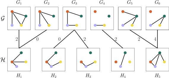
Figure 1: Example of the dtgw-distance between two temporal graphs $\mathcal{G}$ and $\mathcal{H}$ on four vertices with lifetimes six and five. The vertex coloring indicates an optimal vertex mapping $M$. The connections between the boxes indicate an optimal warping path $p=\{(1,1),(2,1),(3,2),(3,3),(4,4),(5,5),(6,5)\}$. Their labels correspond to the costs $C(G_{i},H_{j},M)$ where the vertex signatures are the degrees and the metric is the absolute value of the difference. For example, the cost of warping $G_{1}$ to $H_{1}$ is 2, as the green and yellow vertex each have degree two in $G_{1}$ but only degree one in $H_{1}$. The resulting dtgw-distance is $\operatorname{dtgw}(\mathcal{G},\mathcal{H})=2+0+0+2+2+2+4=12$.

Figure 1 depicts an example illustrating the dtgw-distance of two temporal graphs. Intuitively, the vertex mapping identifies vertices with similar behavior over time and the warping path identifies the time layers with similar vertex behavior. Note that (for $T=U)$ if one fixes $p=\{(1,1),(2,2),\ldots,(T,T)\}$, then we get a temporal graph distance without time warping (similar to the Euclidean distance).

The following results are easily observed and play a central role for our subsequent algorithms.

Observation 3.1.

Let $\mathcal{G}=(V,E_{1},\ldots,E_{T})$ and $\mathcal{H}=(W,F_{1},\ldots,F_{U})$ be two temporal graphs with $\lvert V\rvert\leq\lvert W\rvert\eqqcolon n$.

1. For a fixed vertex mapping $M\in\mathcal{M}(V,W)$, a warping path $p\in\mathcal{P}_{T,U}$ which minimizes $\sum_{(i,j)\in p}C(G_{i},H_{j},M)$ can be computed in $\mathcal{O}(T\cdot U\cdot n)$ time.

2. For a fixed warping path $p\in\mathcal{P}_{T,U}$, a vertex mapping $M\in\mathcal{M}(V,W)$ which minimizes $\sum_{(i,j)\in p}C(G_{i},H_{j},M)$ can be computed in $\mathcal{O}(n^{2}\cdot\lvert p\rvert+n^{3})$ time.

Proof.

$i)$ For a given vertex mapping $M$, an optimal warping path can be computed by a well-known dynamic program for dynamic time warping in $\mathcal{O}(T\cdot U\cdot n)$ time [42]. Here, $\mathcal{O}(n)$ is the time required to compute the costs $C(G_{i},H_{j},M)$. Note that faster dynamic time warping algorithms for special cases are known [1, 19, 32, 14].

$ii)$ Let $V^{\prime}\coloneqq V\cup Q$, where $Q$ is a set of $|W|-|V|$ dummy vertices (that is, $|V^{\prime}|=n$) with $Q\cap V=\emptyset$. For every $(u,v)\in V^{\prime}\times W$, let

$$\sigma(u,v)\coloneqq\begin{cases}\sum_{(i,j)\in p}d\big{(}f_{G_{i}}(u),f_{H_{j}}(v)\big{)},&u\in V\\ \sum_{(i,j)\in p}\Delta_{H_{j}}(v),&u\in Q\end{cases}.$$

Then, we need to find a vertex mapping $M\in\mathcal{M}(V^{\prime},W)$ that minimizes $\sum_{(u,v)\in M}\sigma(u,v)$. Note that $M$ defines a bijection between $V^{\prime}$ and $W$. Hence, computing $M$ is an Assignment Problem instance solvable in $\mathcal{O}(n^{3})$ time [3, Theorem 12.2]. Computing all $\sigma(u,v)$ values can be done in $\mathcal{O}(n^{2}\cdot\lvert p\rvert)$ time. ∎

Note that 3.1 i) implies that if we already know the vertex mapping up to a constant number of vertices, then $\operatorname{dtgw}$ can be computed in polynomial time (since we can try out all polynomially many possible vertex mappings). Furthermore, 3.1 ii) implies that $\operatorname{dtgw}$ is polynomial-time computable if the optimal temporal alignment between $\mathcal{G}$ and $\mathcal{H}$ is known beforehand. In particular, $\operatorname{dtgw}$ can be computed in polynomial time if one temporal graph has a constant lifetime or a constant number of vertices since there are only polynomially many possible warping paths or polynomially many vertex mappings.

Corollary 3.2.

The dtgw-distance between two temporal graphs can be computed in polynomial time if at least one of the following applies:

1. The vertex mapping is known up to a constant number of vertices.

2. The warping path is known.

3. At least one of the temporal graphs has a constant lifetime or a constant number of vertices.

For given vertex signature function and metric, we refer to the decision problem of testing whether two temporal graphs have dynamic temporal graph warping distance at most some given value $c$ by DTGW.

Dynamic Temporal Graph Warping (DTGW)

Input:	Two temporal graphs $\mathcal{G}$ and $\mathcal{H}$, $c\in\mathbb{Q}$.
Question:	Is $\operatorname{dtgw}(\mathcal{G},\mathcal{H})\leq c$?

4 Computational Hardness

Even though the dynamic time warping distance and the vertex-signature-based graph distance are both computable in polynomial time, their combined application to temporal graphs yields a distance measure that is generally NP-hard to compute. Intuitively, this is due to the fact that the vertex mapping has to be consistent for all layers. This introduces non-trivial dependencies between the time warping and the vertex mapping which render the problem computationally hard. Indeed, this is not a singular case for temporal graph problems where for many cases the temporal counterparts of problems solvable in polynomial time turn NP-hard; examples include the computation of matchings in graphs [20, 4, 34], short path computations [6, 12], or the computation of separators [45].

Theorem 4.1.

DTGW is NP-complete for every metric when the vertex signatures are vertex degrees.

Proof.

DTGW is clearly contained in NP since for a given vertex mapping and warping path (both having polynomial size), one can check in polynomial time whether the $\operatorname{dtgw}$-distance is at most $c$ (also see 3.1).

To show NP-hardness, we give a polynomial-time many-one reduction from the NP-complete $3$-SAT problem. Let $d:\mathbb{Q}\times\mathbb{Q}\to\mathbb{Q}$ be any metric and let $\phi=C_{1}\wedge\ldots\wedge C_{m}$ be an instance of $3$-SAT over the variables $x_{1},\ldots,x_{n}$. Each clause $C_{j}$ is then a disjunction of three literals $C_{j}=:\ell_{j}^{1}\lor\ell_{j}^{2}\lor\ell_{j}^{3}$ and there is a function $\nu:[m]\times[3]\to[n]$ such that $\ell_{j}^{i}\in\{x_{\nu(j,i)},\overline{x_{\nu(j,i)}}\}$ holds for all $\ell_{j}^{i}$. Without loss of generality we assume $m>8$.

The idea is to represent each literal by a vertex which can be mapped to either $\top$ (true) or $\bot$ (false). We then build, for each clause, a clause box gadget consisting of three consecutive layers. The choice of a warping path will then, for each clause, implicitly select one of its literals and the costs caused by each clause box will attain their minimum value if and only if that particular literal is mapped to $\top$.

Now a detailed description of the reduction follows. Let $D$ and $D^{\prime}$ be two copies of the graph $\coprod_{i=1}^{22m}K_{2}$ (consisting of $22m$ disjoint edges), where for each vertex $v\in V(D)$ we denote its copy in $V(D^{\prime})$ by $v^{\prime}$. We construct two temporal graphs $\mathcal{G}$ and $\mathcal{H}$. Their vertex sets each contain $2n+47m+8$ vertices as follows.

Both temporal graphs have $2n+26m$ layers defined as follows. For each $i\in[n]$, we set

$$E(G_{2i-1}) \coloneqq\{\{x_{i},\overline{x_{i}}\}\}, E(H_{2i-1}) \coloneqq\{\{\top_{i},\bot_{i}\}\},$$

$$E(G_{2i}) \coloneqq E(D), E(H_{2i}) \coloneqq E(D^{\prime})\,.$$

For $j\in[m]$, we set Figure 5: Sensitivity of dtgw to noise. Shown are the dendograms obtained by agglomerative clustering using complete linkage. Different colors represent different grades, the light gray edges connect elements of different grades. The top left dendogram shows the result obtained by the dtgw-distance. The top right dendogram shows the result obtained by the non-consistent benchmark. The bottom dendogram shows the result obtained by using the non-temporal benchmark.

6.4 De-Anonymization

Besides measuring a distance between temporal graphs, the dtgw-distance additionally provides a mapping between the vertex sets which implicitly allows to identify vertices. This allows the de-anonymization [35] of temporal social networks. Since the data sets used contain the original mapping between the vertext sets, we can employ this as an easy benchmark for the accuracy of the dtgw-distance.

We used the AM heuristic (with shortest warping path initialization) to compute the dtgw-distance (with degrees as vertex signatures) on the three data sets mentioned in LABEL:sec:data. We counted how many vertices were correctly re-identified (that is, mapped to their copies) in the resulting vertex mapping. We compared our results to the following alternative algorithms found in the literature:

• DynaMAGNA++ [43]: A search-based evolutionary algorithm computing a vertex mapping that maximizes edge conservation and node conservation over time.

• Temporal Network Embedding [46]: Hawkes Process Based Temporal Network Embedding (HTNE) computes a low-dimensional embedding of the vertices of a temporal network. From this, we computed a vertex mapping minimizing the Euclidean distances between the vertex feature vectors.

• Fixed dtgw: Note that our dtgw-distance allows to fix the warping path beforehand (3.1 ii)). Since in our case each pair of temporal graphs was recorded using synchronized clocks, it is natural to use a fixed warping path that aligns layer $i$ of the first graph with layer $i$ of the second graph.

To simulate a situation in which the temporal graphs represent processes which do not run synchronously in time, we created two modified versions of each of the data sets. In the first one, called “shifted”, all events of the first graph were delayed by three minutes. In the second version, called “randomized”, each layer of each of the graphs was randomly and independently replaced by $X$ layers where $X\in\{1,2,\dots\}$ is a random variable with $\mathbb{P}(X\geq x)=x^{-3}$. Since we pretend that the nature of these modifications is unknown to the tested algorithms, dtgw with fixed warping path is not applicable to these variants.

For DynaMAGNA++, we used a population of size 15 000 and a maximum of 10 000 generations. With HTNE, we computed 128-dimensional vertex embeddings using a batch of size 10 000, a learning rate of 0.1, a history length of 2, and 5 negative samples. Unlike dtgw, both methods utilized all four processor cores.

The results and running times are listed in Table 1. Most notably, the re-identification rate of HTNE was poor on all data sets, suggesting that these embeddings are ill-suited for comparing vertices taken from different networks. Furthermore, all methods failed to re-identify any significant number of vertices on the primary school data set. This might be explained by the fact that the co-presence network is very different from the face-to-face contacts due to a low spatial resolution (as was also noted by Génois and Barrat [18]).

The overall performance was much better on the other two data sets, especially on the conference data where up to 90% of participants could be re-identified whereas on the workplace data set the best result was 51%. Unsurprisingly, fixing the correct layer alignment on the unmodified graphs sped up the dtgw computation significantly while also yielding slightly better results. On these instances, dtgw performed comparably to DynaMAGNA++, being better in one case and worse in the other, although requiring much less computational effort. In contrast, on the shifted and randomized data sets dtgw always achieved the best results (notably the re-identification performance using dtgw did not decrease on shifted data).

In all cases the AM heuristic converged after at most six iterations and DynaMAGNA++ converged within 2 000 generations.

Table 1: Percentages (rounded) of vertices that were re-identified by the tested methods. Also average running times (in seconds) over the three versions of each data set are given (fixed dtgw is not applicable for shifted and randomized data sets).

	data set	dtgw	fixed dtgw	DynaMAGNA++	HTNE
school	original	2%	1%	1%	1%
	shifted	1%	–	0%	1%
	randomized	1%	–	1%	0%
	average running time	95 s	65 s	15 070 s	250 s
conference	original	86%	90%	80%	0%
	shifted	86%	–	27%	0%
	randomized	65%	–	30%	1%
	average running time	200 s	125 s	20 320 s	90 s
workplace	original	38%	43%	51%	1%
	shifted	38%	–	19%	0%
	randomized	10%	–	8%	1%
	average running time	45 s	20 s	1 600 s	50 s

7 Conclusion

We introduced a new proximity measure for comparing temporal graphs by transferring dynamic time warping from time series to temporal graphs. This yields a challenging computational problem for which we proposed exact algorithms and a heuristic approach to solve it. While exact solutions can only be computed for very small instances, we empirically showed that our heuristic runs fast in practice and yields good approximations of optimal solutions. In our experiments, it was also capable of de-anonymizing social networks.

Our work opens several directions for future research. We believe that the dtgw-distance is a promising tool for example in biology and chemistry. Processes like epidemic disease spreading or chemical reactions can naturally be viewed as temporal graphs where the vertices represent individuals or (macro) molecules (unfortunately we could not test this, as there is still a lack of openly available temporal molecular data [43]). Since the exact time scales of these processes often vary, the ability of dynamic time warping to compensate for such differences would be especially helpful in this context. One might also use the dtgw-distance to understand the learning process of neural networks. The training phases of neural networks yield temporal networks which can be analyzed to gain insight into how different conditions influence the learning process. Another potential application is analyzing team sports data via temporal graphs to reveal similar strategies or roles of individual players. Depending on the application domain, there is a wide range of possibilities to test the performance when using different vertex signatures or even other graph distances.

Besides experimenting with various application domains and further definition variants, already the proven computational worst-case hardness of DTGW may trigger further algorithmic research. A concrete open question is whether DTGW is in XP (or even fixed-parameter tractable) with respect to $\lambda$, when the warping path length is restricted to be at most $\max(T,U)+\lambda$ where $T$, $U$ are the respective lifetimes. It is also interesting to further study the influence of graph-specific parameters in the spirit of a multivariate complexity analysis [37, 11].

References

- Abboud et al. [2015] A. Abboud, A. Backurs, and V. V. Williams. Tight hardness results for LCS and other sequence similarity measures. In 2015 IEEE 56th Annual Symposium on Foundations of Computer Science (FOCS ’15), pages 59–78, 2015. doi:10.1109/FOCS.2015.14.
- Ahmed and Karypis [2015] R. Ahmed and G. Karypis. Algorithms for mining the coevolving relational motifs in dynamic networks. ACM Transactions on Knowledge Discovery from Data, 10(1):4:1–4:31, 2015. doi:10.1145/2733380.
- Ahuja et al. [1993] R. K. Ahuja, T. L. Magnanti, and J. B. Orlin. Network Flows: Theory, Algorithms, and Applications. Prentice-Hall, 1993. ISBN 978-0-13-617549-0.
- Baste et al. [2020] J. Baste, B.-M. Bui-Xuan, and A. Roux. Temporal matching. Theoretical Computer Science, 806:184–196, 2020. doi:10.1016/j.tcs.2019.03.026.
- Bento and Ioannidis [2018] J. Bento and S. Ioannidis. A family of tractable graph distances. In Proceedings of the 2018 SIAM International Conference on Data Mining (SDM ’18), pages 333–341. SIAM, 2018. doi:10.1137/1.9781611975321.38.
- Casteigts et al. [2019] A. Casteigts, A. Himmel, H. Molter, and P. Zschoche. The computational complexity of finding temporal paths under waiting time constraints. CoRR, 2019. URL http://arxiv.org/abs/1909.06437.
- Cygan et al. [2015] M. Cygan, F. V. Fomin, L. Kowalik, D. Lokshtanov, D. Marx, M. Pilipczuk, M. Pilipczuk, and S. Saurabh. Parameterized Algorithms. Springer, 2015. doi:10.1007/978-3-319-21275-3.
- Dakiche et al. [2019] N. Dakiche, F. B.-S. Tayeb, Y. Slimani, and K. Benatchba. Tracking community evolution in social networks: A survey. Information Processing & Management, 56(3):1084–1102, 2019. doi:10.1016/j.ipm.2018.03.005.
- Downey and Fellows [2013] R. Downey and M. R. Fellows. Fundamentals of Parameterized Complexity. Springer, 2013. doi:10.1007/978-1-4471-5559-1.
- Elhesha et al. [2019] R. Elhesha, A. Sarkar, P. Cinaglia, C. Boucher, and T. Kahveci. Co-evolving patterns in temporal networks of varying evolution. In Proceedings of the 10th ACM International Conference on Bioinformatics, Computational Biology and Health Informatics (BCB ’19), page 494–503. ACM, 2019. doi:10.1145/3307339.3342152.
- Fellows et al. [2013] M. R. Fellows, B. M. P. Jansen, and F. Rosamond. Towards fully multivariate algorithmics: Parameter ecology and the deconstruction of computational complexity. European Journal of Combinatorics, 34(3):541–566, 2013. doi:10.1016/j.ejc.2012.04.008.
- Fluschnik et al. [2020] T. Fluschnik, R. Niedermeier, C. Schubert, and P. Zschoche. Multistage - path: Confronting similarity with dissimilarity. CoRR, 2020. URL http://arxiv.org/abs/2002.07569.
- Froese et al. [2019] V. Froese, B. Jain, R. Niedermeier, and M. Renken. Comparing temporal graphs using dynamic time warping. In Proceedings of the 8th International Conference on Complex Networks and their Applications, volume 882 of SCI, pages 469–480. Springer, 2019. doi:10.1007/978-3-030-36683-4_38.
- Froese et al. [2020] V. Froese, B. J. Jain, and M. Rymar. Fast exact dynamic time warping on run-length encoded time series. CoRR, 2020. URL http://arxiv.org/abs/1903.03003.
- Fröhlich et al. [2005] H. Fröhlich, J. K. Wegner, F. Sieker, and A. Zell. Optimal assignment kernels for attributed molecular graphs. In Proceedings of the 22nd International Conference on Machine Learning (ICML ’05), pages 225–232. ACM, 2005. doi:10.1145/1102351.1102380.
- Garey and Johnson [1979] M. R. Garey and D. S. Johnson. Computers and Intractability: A Guide to the Theory of NP-Completeness. W. H. Freeman and Company, 1979. ISBN 0-7167-1044-7.
- Gayraud et al. [2015] N. T. Gayraud, E. Pitoura, and P. Tsaparas. Diffusion maximization in evolving social networks. In Proceedings of the 2015 ACM Conference on Online Social Networks (COSN ’15), pages 125–135. ACM, 2015. doi:10.1145/2817946.
- Génois and Barrat [2018] M. Génois and A. Barrat. Can co-location be used as a proxy for face-to-face contacts? EPJ Data Science, 7(1):11, 2018. doi:10.1140/epjds/s13688-018-0140-1.
- Gold and Sharir [2018] O. Gold and M. Sharir. Dynamic time warping and geometric edit distance: Breaking the quadratic barrier. ACM Transactions on Algorithms, 14(4):50:1–50:17, 2018. doi:10.1145/3230734.
- Heeger et al. [2019] K. Heeger, A. Himmel, F. Kammer, R. Niedermeier, M. Renken, and A. Sajenko. Multistage problems on a global budget. CoRR, 2019. URL http://arxiv.org/abs/1912.04392.
- Holme and Saramäki [2012] P. Holme and J. Saramäki. Temporal networks. Physics Reports, 519(3):97–125, 2012. doi:10.1016/j.physrep.2012.03.001.
- Holme and Saramäki [2013] P. Holme and J. Saramäki. Temporal Networks. Springer, 2013. doi:10.1007/978-3-642-36461-7.
- Holme and Saramäki [2019] P. Holme and J. Saramäki. Temporal Network Theory. Springer, 2019. doi:10.1007/978-3-030-23495-9.
- Impagliazzo and Paturi [2001] R. Impagliazzo and R. Paturi. On the complexity of -SAT. Journal of Computer and System Sciences, 62(2):367–375, 2001. doi:10.1006/jcss.2000.1727.
- Impagliazzo et al. [2001] R. Impagliazzo, R. Paturi, and F. Zane. Which problems have strongly exponential complexity? Journal of Computer and System Sciences, 63(4):512–530, 2001. doi:10.1006/jcss.2001.1774.
- Jain [2016] B. J. Jain. On the geometry of graph spaces. Discrete Applied Mathematics, 214:126–144, 2016. doi:10.1016/j.dam.2016.06.027.
- Jonker and Volgenant [1987] R. Jonker and A. Volgenant. A shortest augmenting path algorithm for dense and sparse linear assignment problems. Computing, 38(4):325–340, 1987. doi:10.1007/BF02278710.
- Jouili and Tabbone [2009] S. Jouili and S. Tabbone. Graph matching based on node signatures. In Proc. of the 7th IAPR-TC-15 International Workshop on Graph-Based Representations in Pattern Recognition, volume 5534 of LNCS, pages 154–163. Springer, 2009. doi:10.1007/978-3-642-02124-4_16.
- Kostakos [2009] V. Kostakos. Temporal graphs. Physica A: Statistical Mechanics and its Applications, 388(6):1007–1023, 2009. doi:10.1016/j.physa.2008.11.021.
- Kriege et al. [2016] N. M. Kriege, P.-L. Giscard, and R. Wilson. On valid optimal assignment kernels and applications to graph classification. In Advances in Neural Information Processing Systems 29 (NIPS ’16), pages 1623–1631. Curran Associates, Inc., 2016. URL http://papers.nips.cc/paper/6166-on-valid-optimal-assignment-kernels-and-applications-to-graph-classification.
- Kriege et al. [2020] N. M. Kriege, F. D. Johansson, and C. Morris. A survey on graph kernels. Applied Network Science, 5(1):6, 2020. doi:10.1007/s41109-019-0195-3.
- Kuszmaul [2019] W. Kuszmaul. Dynamic time warping in strongly subquadratic time: Algorithms for the low-distance regime and approximate evaluation. In Proceedings of the 46th International Colloquium on Automata, Languages, and Programming (ICALP ’19), volume 132 of LIPIcs, pages 80:1–80:15. Schloss Dagstuhl - Leibniz-Zentrum für Informatik, 2019. doi:10.4230/LIPIcs.ICALP.2019.80.
- Li et al. [2017] A. Li, S. P. Cornelius, Y.-Y. Liu, L. Wang, and A.-L. Barabási. The fundamental advantages of temporal networks. Science, 358(6366):1042–1046, 2017. doi:10.1126/science.aai7488.
- Mertzios et al. [2020] G. B. Mertzios, H. Molter, R. Niedermeier, V. Zamaraev, and P. Zschoche. Computing maximum matchings in temporal graphs. In Proceedings of the 37th International Symposium on Theoretical Aspects of Computer Science (STACS ’20), LIPIcs, pages 27:1–27:14. Schloss Dagstuhl - Leibniz-Zentrum für Informatik, 2020. doi:10.4230/LIPIcs.STACS.2020.27.
- Narayanan and Shmatikov [2009] A. Narayanan and V. Shmatikov. De-anonymizing social networks. In Proceedings of the 30th IEEE Symposium on Security and Privacy, pages 173–187, 2009. doi:10.1109/SP.2009.22.
- Nguyen et al. [2018] G. H. Nguyen, J. B. Lee, R. A. Rossi, N. K. Ahmed, E. Koh, and S. Kim. Continuous-time dynamic network embeddings. In Companion Proceedings of the The Web Conference 2018 (WWW ’18), pages 969–976. International World Wide Web Conferences Steering Committee, 2018. doi:10.1145/3184558.3191526.
- Niedermeier [2010] R. Niedermeier. Reflections on Multivariate Algorithmics and Problem Parameterization. In Proceedings of the 27th International Symposium on Theoretical Aspects of Computer Science (STACS ’10), volume 5 of LIPIcs, pages 17–32. Schloss Dagstuhl–Leibniz-Zentrum fuer Informatik, 2010. doi:10.4230/LIPIcs.STACS.2010.2495.
- Rakthanmanon et al. [2012] T. Rakthanmanon, B. Campana, A. Mueen, G. Batista, B. Westover, Q. Zhu, J. Zakaria, and E. Keogh. Searching and mining trillions of time series subsequences under dynamic time warping. In Proceedings of the 18th ACM SIGKDD International Conference on Knowledge Discovery and Data Mining (KDD ’12), pages 262–270. ACM, 2012. doi:10.1145/2339530.2339576.
- Riesen [2015] K. Riesen. Structural Pattern Recognition with Graph Edit Distance. Springer, 2015. doi:10.1007/978-3-319-27252-8.
- Rozenshtein and Gionis [2019] P. Rozenshtein and A. Gionis. Mining temporal networks. In Proceedings of the 25th ACM SIGKDD International Conference on Knowledge Discovery & Data Mining (KDD ’19), pages 3225–3226. ACM, 2019. doi:10.1145/3292500.3332295.
- Rozenshtein et al. [2016] P. Rozenshtein, A. Gionis, B. A. Prakash, and J. Vreeken. Reconstructing an epidemic over time. In Proceedings of the 22nd ACM SIGKDD International Conference on Knowledge Discovery and Data Mining (KDD ’16), pages 1835–1844. ACM, 2016. doi:10.1145/2939672.2939865.
- Sakoe and Chiba [1978] H. Sakoe and S. Chiba. Dynamic programming algorithm optimization for spoken word recognition. IEEE Transactions on Acoustics, Speech, and Signal Processing, 26(1):43–49, 1978. doi:10.1109/TASSP.1978.1163055.
- Vijayan et al. [2017] V. Vijayan, D. Critchlow, and T. Milenković. Alignment of dynamic networks. Bioinformatics, 33(14):i180–i189, 2017. doi:10.1093/bioinformatics/btx246.
- Wang et al. [2013] X. Wang, A. Mueen, H. Ding, G. Trajcevski, P. Scheuermann, and E. Keogh. Experimental comparison of representation methods and distance measures for time series data. Data Mining and Knowledge Discovery, 26(2):275–309, 2013. doi:10.1007/s10618-012-0250-5.
- Zschoche et al. [2020] P. Zschoche, T. Fluschnik, H. Molter, and R. Niedermeier. The complexity of finding small separators in temporal graphs. Journal of Computer and System Sciences, 107:72–92, 2020. doi:10.1016/j.jcss.2019.07.006.
- Zuo et al. [2018] Y. Zuo, G. Liu, H. Lin, J. Guo, X. Hu, and J. Wu. Embedding temporal network via neighborhood formation. In Proceedings of the 24th ACM SIGKDD International Conference on Knowledge Discovery and Data Mining (KDD ’18), pages 2857–2866. ACM, 2018. doi:10.1145/3219819.3220054.