Stable target opinion through power law bias in information exchange

Abstract

We study a model of binary decision making when a certain population of agents is initially seeded with two different opinions, ‘$+$’ and ‘$-$’, with fractions $p_{1}$ and $p_{2}$ respectively, $p_{1}+p_{2}=1$. Individuals can reverse their initial opinion only once based on this information exchange. We study this model on a completely connected network, where any pair of agents can exchange information, and a two-dimensional square lattice with periodic boundary conditions, where information exchange is possible only between the nearest neighbors. We propose a model in which each agent maintains two counters of opposite opinions and accepts opinions of other agents with a power law bias until a threshold is reached, when they fix their final opinion. Our model is inspired by the study of negativity bias and positive-negative asymmetry known in the psychology literature for a long time. Our model can achieve stable intermediate mix of positive and negative opinions in a population. In particular, we show that it is possible to achieve close to any fraction $p_{3},0\leq p_{3}\leq 1$, of ‘$-$’ opinion starting from an initial fraction $p_{1}$ of ‘$-$’ opinion by applying a bias through adjusting the power law exponent of $p_{3}$.

I I. Introduction

The study of emergent behaviour in a population based on simple interaction rules among individuals has been an intense area of research in complex systems and sociophysics. Most of these models study opinion formation in a population in the context of two different opinions, majority and minority, or ‘$+$’ and ‘$-$’. The opinions in these models evolve either according to some simple local rules, or according to some group dynamics. An extensive review of such models can be found in the paper by Castellano et al.CFL .

The aim of this paper is to investigate negativity bias in opinion formation. There is an extensive literature on negativity bias in psychology, as reviewed by Rozin and Royzman RR and Vaish et al. VGW . Negativity bias is manifested in humans and animals in many different activities, including, attention and salience, sensation and perception, motivation, mood and decision making RR . Some of these activities are closely related to opinion formation and hence, it is interesting to study the effect of negativity bias in opinion formation in a population. We present a model of opinion formation that uses negativity bias and has several interesting properties, including a similarity with the random-field Ising model and also the formation of predictable intermediate configurations of mixed opinions.

One of the earliest among opinion formation models was the voter model (VM) L ; LI that can be simulated on any connected network. Each agent has a state $\pm 1$ and two neighboring agents interact at each simulation time step. Starting from a ($+-$) state, the probablity of assuming a ($++$) or a ($--$) state in an interaction is $\frac{1}{2}$ each. This simple update rule gives rise to rich dynamical behavior and the VM has been studied extensively. The VM always evolves to a homogeneous final state of one of the opinions, the rate of convergence depends on the initial populations of the two opinions, and has a stochastic nature. Hence it is hard to predict the mix of populations at intermediate stages of the evolution.

Schweitzer and Behera SB introduced the nonlinear VM where neighbors with different opinions are weighted with nonlinear weighting factors. The nonlinear VM has interesting configurations where both the opinions coexist equally when the starting initial fraction of population for each opinion is $0.5$ of the total. However it is not clear whether the nonlinear VM has any stable intermediate configurations where both opinions coexist if the initial populations are unbalanced.

A contrarian has a different strategy from the other agents. Contrarians introduce interesting variations in the evolution of almost all the models we discuss. Masuda M studied the linear VM by introducing three types of contrarians and concluded that contrarians prevent the evolution of the linear VM to a homogeneous final state of a single opinion and induce a mixed population of both the opinions. Masuda M derived the equilibrium distributions of the two opinions under different assumptions on the contrarians. However it is not clear whether it is possible to get specific mix of populations in the model in M and also whether the dynamics of the model is scale invariant.

Group dynamics of binary opinion formation has been studied by Galam and his coworkers extensively as discussed in the review paper G . Galam’s G1 2-state opinion dynamics model is of particular interest for our present work. This model is for a completely connected network where any agent is a neighbor of any other agent. Initially each agent has one of two opinions A and B, and the density of the two populations is denoted by $p_{c}$, expressed as a fraction, e.g., $p_{c}=\frac{1}{2}$ indicates a balanced initial population of agents with A and B opinions. Each step of the evolution of the model consists of picking a random group of agents of a predermined size. All agents in this group adopt the opinion of the local majority. When this update process is repeated, the resulting dynamics is dependent on $p_{c}$. The final population is a balance of A and B opinions when $p_{c}=\frac{1}{2}$ and the group size is odd. When the group size is even, the final population is balanced for a different value of $p_{c}$, however, any deviation from these $p_{c}$ values makes the final population to converge to one of the two opinions. The speed of convergence is faster for larger group sizes.

Galam G1 also considered the introduction of contrarian agents in this model, the contrarians participate in the group opinion formation exactly in the same way as before, however, a contrarian reverses its opinion once it has left the group. A mixed phase dynamics with a clear separation of majority and minority opinions prevails when the density of the contrarians $a_{c}$ is low. These populations are stable for a fixed value of $a_{c}$. However, there are thresholds for $a_{c}$ for different group sizes when no opinion dominates and there is no symmetry breaking to separate the final population into majority and minority opinions. In other words the final population is balanced between the two opinions even though agents change their opinion dynamically. It is not clear whether Galam’s model can achieve arbitrary and stable proportions of the two opinions by introducing contrarians.

The Majority Rule (MR) model was introduced by Krapivsky and Redner KR as a simple two-state opinion dynamics model. The MR model has similarities with Galam’s model G1 . A group of agents is chosen at every step and the agents in the group all assume the opinion of the local majority. The aim in KR was to study the time to reach global consensus as a function of $N$, the total number of agents and also the probability of reaching a given final state as a function of the initial opinion densities. The MR model has many interesting properties and one of the characteristics features of the MR model that is of interest to us is that even small islands of one opinion surrounded by the opposite opinion can grow in size. The growth of a particular opinion varies from one initialization to another. There are also intermediate metastable states in the MR model that persist for long times, however again the concentration of opinions in these metastable states vary depending on the initialization.

There are some similarities between our proposed model and the model in G1 . First, the aim of our model is to arrive at a final population of a mixed majority and minortiy population. This is achieved in Galam’s model when the density of the contrarians is low. Second, our model behaves similar to Galam’s model when the fraction of initial population of agents is balanced, i.e., $\frac{1}{2}$ each. This is manifested in Galam’s model both in the absence of contrarians and also when the initial population of contrarians is greater than a threshold for different group sizes.

However there are distinct dissimilarities between our model and the model in G1 , apart from the fact that the update rules in Galam’s model are based on groups. Our aim is to achieve a final population of agents separated into majority and minority opinions without the use of contrarians. In other words, all agents in our model have a common strategy. Galam’s model without contrarians has been analysed for $d$-dimensional lattices by Lanchier and Taylor LT . They have proven that Galam’s model (or the spatial public debate model in the terminology of LT ) converges to a stationary distribution where both the opinions have positive densities. However it is not clear whether any specific mix of the two opinions can be achieved. Our model on the other hand behaves in a similar way both on a completely connected network and on a 2D lattice with nearest neighbor connections. Hence our model can be thought of as the formation of global opinion through simple local interactions. The differnces between our model and the MR model are also similar to the differences mentioned above.

We frame our problem in this paper in a general way as follows. Given an initial population of agents with ‘$+$’ and ‘$-$’ opinions, with fractions $p_{1}$ and $p_{2}$ respectively, $p_{1}+p_{2}=1$, the goal is to achieve a fraction $p_{3}$ of final population of agents with the ‘$-$’ opinion, $0\leq p_{3}\leq 1$, and $p_{3}>p_{2}$. We show that it is possible to achieve close to a final fraction $p_{3}$ of agents with ‘$-$’ opinion by introducing a bias in the exchange of opinion when two agents meet. It is interesting that this bias can be expressed as a power law exponent of $p_{3}$, and scale-invariant for both the completely connected network and the two dimensional lattice. Our model has interesting properties that are similar to other models studied in statistical mechanics. For example, a coexistence of opposite opinions has been observed in the nonlinear voter model SB , even though this coexistence is not stable and predictable in terms of the exact mix of the two opinions. Also properties of our model related to the surface tension of the domain boundaries of opposite opinions and also first-order phase transition and domain formation are similar to the random-field Ising model CN .

The rest of the paper is organized as follows. We discuss our model in section II. We discuss the results from an empirical study of the model without and with the power-law bias during information exchange in sections III and IV respectively. Finally we conclude in section V.

II II. The model

A population initially has agents with two opinions in certain fractions $p_{1}$ and $p_{2}$, with $p_{1}+p_{2}=1$. Each agent has the option of choosing one of the opinions as their final opinion, however, reverting an initial opinion is allowed only once. Agents interact pairwise either on a completely connected network or on a square lattice with periodic boundary conditions. We have two free parameters in our model, $\beta$ and $\tau$. Each agent maintains two counters $\theta^{+}$ and $\theta^{-}$ of the positive and negative opinions encountered so far. Initially $\theta^{+}_{i}=1$ and $\theta^{-}_{i}=0$ if agent $i$ is a ‘$+$’ agent, and $\theta^{+}_{i}=0$ and $\theta^{-}_{i}=1$ if agent $i$ is a ‘$-$’ agent. When agents $i$ and $j$ interact, the rules for exchange of opinion from agent $i$ to agent $j$ are given in eqn.(1) and eqn.(2) (the subscripts of the two counters indicate which agent the counter belongs to):

$$if\;\;(\theta^{-}_{i}>p_{3}^{\beta}\theta^{+}_{i})\;\;then\;\;\theta^{-}_{j}=\theta^{-}_{j}+1$$ (1)

$$if\;\;(\theta^{+}_{i}>\theta^{-}_{i})\;\;then\;\;\theta^{+}_{j}=\theta^{+}_{j}+1$$ (2)

The update of the state of agent $j$ occurs due to one of these two equations in a Monte Carlo step. First eqn.(1) is checked and if it is satisfied and an update occurs, eqn.(2) is skipped for that Monte Carlo step. Otherwise the condition in eqn.(2) is checked and an update occurs if the condition in eqn.(2) is satisfied. There is no exchange of information if $\theta^{+}_{i}=\theta^{-}_{i}$ and the encounter is considered a failure. In other words, we introduce an asymmetry in the updating of the counters of agent $j$ by introducing the bias factor $p_{3}^{\beta}$ in eqn.(1). The other free parameter $\tau$ is used as a threshold of opinion until which an agent participates in information exchange. Once either of the counters $\theta^{+}_{i}$ or $\theta^{-}_{i}$ reaches $\tau$, agent $i$ freezes its state either to ‘$+$’, or to ‘$-$’, depending on whether $\theta^{+}_{i}>\theta^{-}_{i}$ or $\theta^{+}_{i}<\theta^{-}_{i}$. Hence this freezing of state may require a flipping of the initial state of agent $i$, this is allowed only once. Once frozen, the state of agent $i$ remains the same until all agents have reached the threshold which is same for all agents. However agent $i$ still maintains its two counters $\theta^{+}_{i}$ and $\theta^{-}_{i}$ for use in interactions with agents who have not yet reached the threshold $\tau$. Though there are no contrarian agents in our model, the $\beta$ parameter can be viewed as similar to a contrarian strategy as it introduces a bias in the interactions among the agents.

The hallmark of negativity bias is to give greater emphasis to negative perceptions and entities. This emphasis is manifested in four different ways RR , negative potency, steeper negative gradients, negativity dominance and negative differentiation. We aim to capture negative potency and steeper negative gradient in our model. Negative potency gives a stronger impact for negative entities, compared to positive entities. This is captured in eqn (1). Negative gradient emphasises the steeper growth of negative events compared to positive events. This is an outcome of our model as we will explain in later sections. It becomes harder for positive opinion to prevail as negative opinion accummulates more and more in the counters of the agents in our model. The use of a single exponent in the power law bias for the whole population tries to capture the inherent negativity bias quantitatively through a single exponent. Though this is a simplified assumption in eqn.(1), we show later that the behavior of the system is quite stable when this exponent is allowed to vary randomly within a certain range.

The agents in our model maintain more information compared to Galam’s model G1 and the MR model KR in the sense that an agent has access to both accumulated positive and negative opinions of another agent during an interaction. It may seem that we are assuming a lot more information for decision making, However one surprising aspect of our model is that the convergence to the desired final state is very fast. In other words, each agent needs to interact with a much smaller number of other agents in order to arrive at a ‘correct’ decision, so that the overall fraction of desired opinion is achieved. Also our model can converge to a desired ‘$-$’ opinion above the $0.5$ threshold accurately even when the initial fraction of agents with ‘$-$’ opinion is low. This is not the case for all the models that we have reviewed above. Galam’s model G1 can achieve such a target population only by using contrarian agents. The MR model has intermediate states with mixed populations, however the mix is sensitive to instances of the two initial populations even when the fraction of the two initial populations are fixed.

We will show in the following sections that our model has stable states of mix of opinions that can be tuned fairly accurately using the $\beta$ and $\tau$ parameters. These stable states are scale-invariant both for the completely connected network and the 2D lattice. However our model is unstable with respect to the $\tau$ parameter. The final configurations converge to a single opinion if the threshold $\tau$ is set relatively high. This convergence is faster on the completely connected network and much slower on the 2D lattice. However, the parameter $\tau$ is a measure of the number of interactions among the agents and a lower value indicates that the convergence of our model to a balanced population mix is faster.

Forming opinion based on accumulated history may be a realistic model in the sense that people in real life accept others’ opinions for decision making. Also people have their own opinion and they usually take others’ opinions with some negativity bias. The contagious effects of negative opinions has been studied in the psychology literature RR , and it has been noted that negative aspects of human thought process spread faster RN . Moreover people discussing a binary opinion usually talk about the pros and cons of the two choices. Though it is hard to capture these processes through some numerical estimates, agents in our model abstract such real-life interactions and discussions through the counters and also through the bias for accepting opinions.

Figure 1: Two simulation results on a $256\times 256$ lattice, ‘$-$’ agents are shown in black and ‘$+$’ agents in white, simulation time ($t$) is measured in Monte Carlo (MC) steps. (a) Initial fractions of populations: ‘$+$’ and ‘$-$’ both $0.5$ of the total; (b) The lattice after all agents reach the threshold $\tau=10$, at $t=2657346$. The final population of ‘$-$’ agents was a fraction of $0.51$ of the total; (c) Initial fractions of populations: ‘$-$’opinion $0.7$ and ‘$+$’ opinion $0.3$; (d) The lattice after all agents reach the threshold $\tau=10$, at $t=2500178$. The final population of ‘$-$’ agents was a fraction of $0.9$ of the total.

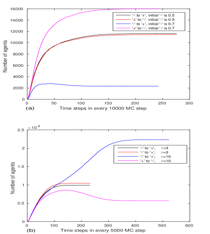
Figure 2: The conversion of agents from ‘$+$’ to ‘$-$’ and ‘$-$’ to ‘$+$’. (a) On a $256\times 256$ lattice, corresponding to the simulations in Fig. 1. The middle two plots are for the simulation when the initial population is balanced, $0.5$ each of ‘$+$’ and ‘$-$’ agents. The top and bottom plots are for an initial population of ‘$-$’ agents $0.7$ of the total. The conversion of ‘$+$’ to ‘$-$’ is much higher (top plot), compared to the conversion of ‘$-$’ to ‘$+$’ (bottom plot). (b) On a completely connected network (CCN). The two middle plots are for a small threshold $\tau=3$, and the conversions are similar. The conversions vary widely from run to run (bottom and top plots) when the threshold is higher ($\tau=10$).

III III. Dynamics without bias

We first discuss the dynamics of our model without applying any bias, in other words when $\beta=0$ in eqn.(1). There is no bias for ‘$+$’ or ‘$-$’ opinion in this case, and agent $j$ accepts the higher of the two counters $\theta^{+}_{i}$ and $\theta^{-}_{i}$ of agent $i$ for updating its own counter. We study some interesting dynamics of our model on a $256\times 256$ lattice in Fig. 1. We have verified that these results are scale-invariant by simulating them on lattices of size $512\times 512$ and $1024\times 1024$.

Fig.1 shows results of two simulations of the unbiased system on a $256\times 256$ lattice with wrap-around connections. Panels (a) and (b) show the results when the initial populations of ‘$+$’ and ‘$-$’ agents are a fraction of $0.5$ each, and the threshold is $\tau=10$. We have simulated this configuration $100$ times and the final fraction of ‘$-$’ agents is between $0.48-0.52$ in all the simulations. Panel (a) shows the initial population of the agents ($t=0$), black (resp. white) denotes ‘$-$’ (resp. ‘$+$’) agents. In panel (b), all agents reach the threshold by $t=2657346$.

Since the final fractions of ‘$+$’ and ‘$-$’ agents are almost the same, the basic difference between panels (a) and (b) is the rearrangements of the agents into clusters. Panels (c) and (d) in Fig.1 are for a simulation when the initial population of ‘$-$’ agents is $0.7$ of the total. Cluster formation is more pronounced in this simulation. The final fraction of ‘$-$’ agents in panel (d) is $0.9$ with a variation of $\pm 0.02$ for $100$ simulations. We note here that the behavior of our model has some similarity with the nonlinear voter model SB in this aspect of cluster formation.

Fig.2 shows the conversion of agents from ‘$-$’ to ‘$+$’ and vice versa. Panel (a) in Fig.2 shows this conversion for the simulations in Fig.1 on a $256\times 256$ lattice. We have plotted these graphs by counting agents that had an initial ‘$-$’ opinion, but had $\theta^{+}>\theta^{-}$ at a particular simulation step, or vice versa. The error bars are very small compared to the values of the data points, hence they are not shown. When the initial populations are balanced, the conversions are almost in equal numbers and the conversions stop at around $t=1500000$, thereafter the agents remain either ‘$+$ or ‘$-$’ and gradually reach their thresholds. This implies a rearrangement of the agents in distinct clusters similar to the first order phase transition in a 2D random-field Ising model C .

When the simulation starts with an initial fraction $0.7$ of ‘$-$’ agents, the final fraction of ‘$-$’ agents is $0.9$ with a variation of $\pm 0.02$ for $100$ simulations. The conversion of ‘$+$’ to ‘$-$’ agents in this case is much higher and the fraction of ‘$-$’ agents increases from a fraction of $0.7$ to over $0.9$. However, still there are some conversions from ‘$-$’ to ‘$+$’ agents. The final configuaration at $t=2500178$ shows islands of ‘$+$’ agents due to strong surface tension.

Panel (b) in Fig.2 shows similar conversions of agents for a simulation on a completely connected network (CCN) of size $65536$. These simulations are very sensisitive to the value of $\tau$. Both the simulations have an initial fraction of ‘$-$’ agents as $0.5$, increasing the value of $\tau$ quickly pushes the final population to either all ‘$-$’ or all ‘$+$’ agents and this final population differs from simulation to simulation. The final population is an equal mix of ‘$-$’ and ‘$+$’ agents for $\tau=3$.

The formation of clusters on the lattice is symptomatic in our model, as there is strong surface tension along the boundaries between regions of ‘$-$’ and ‘$+$’ opinions. We also exerimentally verified the surface tension in our model by seeding a lattice of size $256\times 256$ with a droplet of negative opinion and let the system evolve until all the agents reach their thresholds, as shown in Fig. 3. There was almost no change in the shape of the droplet except for minute changes on the boundary. This is different from the voter model, as the coarsening of a similar droplet under the voter model results due to lack of surface tension and the droplet disintegrates into a region with an irregular boundary DCCH .

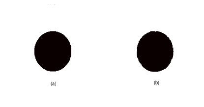
Figure 3: Time evolution of a droplet of ‘$-$’ agents in our model. (a) t=0; (b) t=1985384.

The effects of threshold in our model for a completely connected network and for a lattice are quite different. Increasing the threshold for the lattice has a much slower effect. This we can again attribute to the strong surface tension in our model. The formation of the clusters or islands of ‘$-$’ agents is fairly rapid irrespective of the threhsold and the main effect of the threshold is the increase in convergence time when all the agents reach their thresholds within the clusters. On the other hand the model converges to an all ‘$-$’ or all ‘$+$’ population with higher threshold for the completely connected network.

We studied the formation of clusters of ‘$+$’ and ‘$-$’ agents on a lattice. The clusters of ‘$+$’ and ‘$-$’ agents are of similar size when the starting population of ‘$+$’ and ‘$-$’ agents is $0.5$ of the total population each. The internal sites of clusters have all their neighbors as ‘$+$’ or ‘$-$’ sites, whereas the sites on the surface of clusters have a mixed number of ‘$+$’ and ‘$-$’ neighbors. In Fig.4(a) we study the change in the population of lattice points with different numbers of ‘$+$’ and ‘$-$’ neighbors on a lattice of size $1024\times 1024$. The trends for both ‘$+$’ and ‘$-$’ neighbors are similar. In Fig.4(a), the number of ‘$+$’ sites with a single ‘$-$’ neighbor grows very fast and stabilizes at a high level as more and more lattice sites become parts of larger clusters. These ‘$+$’ sites with a single ‘$-$’ neighbor are on the surface or the boundary of the clusters. On the other hand the number of ‘$+$’ sites with two to four ‘$-$’ neighbors decrese rapidly and stabilize at lower levels, as these sites become parts of clusters.

We study a ratio $\phi$ in Fig.4(b). This is the ratio of lattice sites on the cluster boundaries (sites that have neighbors of opposite opinion) and the total number of possible neighbors in the entire lattice. We have plotted three graphs with starting populations of ‘$-$’ agents as $0.1$, $0.2$ and $0.4$, with varying target populations of ‘$-$’ agents (a fraction of $0.1$ higher than the starting population, until a fraction of $0.9$). The graphs have a general trend that $\phi$ decreases with an increase in the target fraction, as the clusters of ‘$+$’ agents decrease in size. However there is a slight increase in $\phi$ as the starting population of ‘$-$’ agents is increased. This is due to formation of a higher number of ‘$-$’ clusters as a higher initial population provides a larger number of seeds for these clusters.

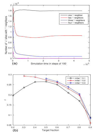
Figure 4: (a) A plot of change of numbers of ‘$+$’ and ‘$-$’ neighbors of lattice sites for a simulation on a lattice of size $1024\times 1024$. The simulation has been done only partially until the clusters stabilize. The top line shows a rapid increase of ‘$+$’ sites that have one ‘$-$’ neighbor. The number of ‘$+$’ sites with two, three and four ‘$-$’ neighbors (second from top to bottom) decrease. (b) $\phi$ against target fraction for three different initial populations of ‘$-$’ agents.

As the ‘$+$’ and ‘$-$’ agents form clusters quite rapidly in simulations on a lattice, it is natural that most of the agents will be inside the clusters and a relatively small number of agents will be on the surface or the boundary of the clusters. This behavior of our model is quite similar to the random-field Ising model CN in this respect. Moreover there is a power-law relationship between the lattice points inside the clusters and on the surface of the clusters. If we denote the number of lattice sites inside the clusters (resp. on the surface) as $V$ (resp. $S$), this relationship can be expressed as

$$S=cV^{\delta}$$ (3)

Figure 5: A log-log plot of surface versus internal points in clusters for different sizes of lattice. The size of the lattice increases from $128\times 128$ (bottom) to $1024\times 1024$ (top).

We show the log-log plot of this equation in Fig. 5 for different sizes of lattice. A data collapse shows that the exponent $\delta=-0.29$ in case of the simulation with initial fraction of ‘$+$’ and ‘$-$’ agents $0.5$ each. The exponent $\delta$ depends on the initial population of ‘$+$’ and ‘$-$’ agents. For example, with a simulation starting with $0.3$ ‘$-$’ and $0.7$ ‘$+$’ agents, the final population of ‘$+$’ agents is $0.8\pm 0.02$ and $\delta=-0.59$. This is due to the fact that the number of clusters of ‘$-$’ agents as well as the sizes of the clusters are smaller in this case and hence the lattice sites on the cluster surfaces are also much smaller in number.

IV IV. Dynamics with bias

Our aim in this section is to use a power-law bias to increase the population of ‘$-$’ agents when the starting population of ‘$-$’ agents is $<0.5$ and the target population of ‘$-$’ agents is higher than the starting population. As we have noted in the previous section the conversion of agents from ‘$+$’ to ‘$-$’ and vice versa is rapid in the early stages of the simulation both for the completely connected network and the lattice. The purpose of introducing the power-law bias in eqn.(1) is to influence this conversion so that a larger proportion of ‘$+$’ agents convert to ‘$-$’ opinion. In eqn.(1), $0\leq p_{3}\leq 1$ and $\beta\geq 0$, and we have discussed the case $\beta=0$ in the previous section. Hence for a fixed $p_{3}$, $p_{3}^{\beta}$ is a monotonically decreasing function of $\beta$. The condition $\theta^{-}_{i}>p_{3}^{\beta}\theta^{+}_{i}$ in eqn.(1) ensures that this condition will be satisfied for lower values of $\theta^{-}_{i}$ compared to $\theta^{+}_{i}$, as the factor $p_{3}^{\beta}<1$ and reduces the magnitude of the right hand side in eqn.(1).

We consider the $\tau$ discrete integer values of $\theta^{-}_{i}$, i.e., $\theta^{-}_{i,1},\theta^{-}_{i,2},\dots,\theta^{-}_{i,\tau}$ for a fixed threshold $\tau$. Similarly we consider the $\tau$ discrete integer values of $\theta^{+}_{i}$, namely, $\theta^{+}_{i,1},\theta^{+}_{i,2},\dots,\theta^{+}_{i,\tau}$. The effect of the factor $p_{3}^{\beta}$ on $\theta^{+}_{i}$ is a mapping $\theta^{+}_{i}\rightarrow\theta^{-}_{i}$ to partition the values $\theta^{+}_{i,1},\theta^{+}_{i,2},\dots,\theta^{+}_{i,\tau}$ into $k$ partitions $P_{k},1\leq k\leq\tau$. The members of partition $P_{m}$ are mapped within two consecutive integer values in $\theta^{-}_{i}$. For example, if we assume $\tau=10,p_{3}=0.9$, and $\beta=2.6$, $p_{3}^{\beta}=0.76$. There are $10$ values each for $\theta^{-}_{i}$ and $\theta^{+}_{i}$, the integers $1,2,\dots,10$. Hence $p_{3}^{\beta}\theta^{+}_{i}$ can be partitioned into eight partitions that are within consecutive integer values of $\theta^{-}_{i}$, $[0,1]_{[1]}$, $[1,2]_{[2]}$, $[2,3]_{[3]}$, $[3,4]_{[4,5]}$, $[4,5]_{[6]}$, $[5,6]_{[7]}$, $[6,7]_{[8,9]}$, $[7,8]_{[10]}$. For example, $[6,7]_{[8,9]}$ indicates that $p_{3}^{\beta}\theta^{+}_{i}$ is between $6$ and $7$ for $\theta^{+}_{i}=8,9$ ($0.76\times 8=6.08$ and $0.76\times 9=6.84$). The dynamics of our model remains unaffected for different values of $\beta$ that result in the same partitions, as the condition in eqn.(1) will evaluate identically for the same partition. In this example $\beta=2.7$ also gives the same partitions for $p_{3}^{\beta}\theta^{+}_{i}$ as $\beta=2.6$, and hence the behavior of our model will remain the same for either of these two choices for $\beta$. Consequently the exponent $\beta$ has a range instead of a unique value for achieving a final population of ‘$-$’ agents and there is no change in the final population when the $\beta$ value remains within this range. However the changes in the final population are sharp whenever the $\beta$ parameter causes a transition from one partition to another.

When the groups of $p_{3}^{\beta}$ are compressed within lower values of $\theta^{-}_{i}$, the result is an increase of the $\theta^{-}_{j}$ counter as the condition in eqn.(1) is satisfied even for lower values of $\theta^{-}_{i}$. As a result this favors the ‘$-$’ agents to dominate the dynamics as more and more agents (both with initial ‘$+$’ or ‘$-$’ opinions) reach their thresholds for the $\theta^{-}$ counters. Hence a high enough threshold makes the system to converge in an all ‘$-$’ opinion scenario. This convergence is faster for the completely connected network compared to the lattice, as the erosion of the surface of the clusters of ‘$+$’ nodes is a much slower process for the lattice.

IV.1 A. Dynamics on a completely connected network

We first study the dynamics of the system through an example for the completely connected network when the initial fraction of ‘$-$’ (resp. ‘$+$’) agents is $0.3$ (resp. $0.7$) of the total population and the required final fraction of ‘$-$’ agents is $0.9$ of the total population. As we have noted earlier, if we simulate this scenario without a bias, i.e., when $\beta=0$, the final fraction of agents with ‘$-$’ opinion reduces further. Also, the final fraction depends on the threshold, it approaches $0$ very fast as the threshold is increased for the completely connected network. On the other hand a low threshold does not allow enough scope for the conversion of a large number of ‘$+$’ agents to ‘$-$’ agents that is required for achieving a high fraction of ‘$-$’ agents starting from a low fraction. This trade-off for the threshold exists for the model with a bias as well. In this case the bias gives an impetus for reversing ‘$+$’ agents to ‘$-$’ agents. If the threshold is high, eventually all ‘$+$’ agents will be converted and the final population will consist of all ‘$-$’ agents.

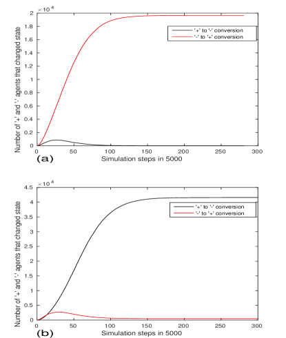
Figure 6: The conversion of agents from ‘$+$’ to ‘$-$’ and ‘$-$’ to ‘$+$’ for the biased and unbiased models for a simulation of $256\times 256=65536$ agents on a completely connected network. $\tau=5$ and $p_{3}=0.9$. The starting population of ‘$-$’ agents is $0.3$ of the total in both cases. If $\theta^{-}_{i}>\theta^{+}_{i}$, agent $i$ is identified as a ‘$-$’ agent, and vice versa. (a) $\beta=0$ and almost all ‘$-$’ agents are converted to ‘$+$’ agents (the upper curve), conversion of ‘$+$’ to ‘$-$’ is very low (lower curve). (b) $\beta=6.7$ and the bias forces conversion of a large number of ‘$+$’ agents to ‘$-$’ (upper curve), compared to ‘$-$’ to ‘$+$’ conversion (lower curve).

Fig. 6 shows the comparison between the simulations of our model with and without bias. This simulation has been done on a completely connected network of $65536$ agents. The starting population of ‘$-$’ agents is a fraction $0.3$ of the total, and the final target population of ‘$-$’ agents is a fraction of $0.9$ of the total population. The threshold $\tau=5$ in this case. The simulation has been done without bias in (a), and a lower starting population of ‘$-$’ agents drives the system to a final population of all ‘$+$’ agents. We show in Fig.6(a) the conversion of agents from ‘$+$’ to ‘$-$’ and vice versa. There is a small initial conversion of ‘$+$’ agents to ‘$-$’, however, soon the larger population of ‘$+$’ agents dominate and all of the initial fraction of $0.3$ of ‘$-$’ agents convert to ‘$+$’. The graph shows a cumulative number of the agents that have higher value in the $\theta^{+}$ or $\theta^{-}$ counter until a particular step. Almost all the conversions occur in the initial stages of the simulation and the agents reach their thresholds afterwards over many simulation steps (as indicated by the red curve in (a)). The biased simulation is shown in (b). The bias in this case drives a conversion of ‘$+$’ agents to ‘$-$’, and as a result the final population of ‘$-$’ agents rise to a fraction of $0.9\pm 0.03$ for $100$ simulations.

The threshold for both the simulations is $\tau=5$. Increasing this threshold for the simulation with bias quickly pushes the final population to consist only of ‘$-$’ agents as a higher threshold gives more scope for ‘$-$’ agents to convert ‘$+$’ agents. For example a simulation with $\tau=10$ has a final population of all ‘$-$’ agents. As $\beta=6.7$ in the simulations in (b), and the final target fraction of ‘$-$’ agents is $p_{3}=0.9$, the bias factor $p_{3}^{\beta}=0.9^{6.7}=0.493$. Since $\tau=5$, there are three partitions of $p_{3}^{\beta}\theta^{+}_{i}$ for agent $i$. These are $[0,1]_{[1,2]}$, $[1,2]_{[3,4]}$ and $[2,3]_{[5]}$. Most of the transitions from ‘$+$’ to ‘$-$’ occur in the initial steps of the simulation as shown in Fig. 6. There is a small number of conversions from ‘$-$’ to ‘$+$’ as well, however, both of these conversions plateau realtively early in the simulation. Another interesting aspect of the dynamics is that a complete coversion of ‘$+$’ to ‘$-$’ agents is dependent on $\tau$, rather than $\beta$, as mentioned earlier. For example, $\beta=18$ gives only one partition of $p_{3}^{\beta}\theta^{+}_{i}$, $[0-1]_{[1-5]}$. However, simulations in this case show a final population of ‘$-$’ agents as a fraction $0.95\pm 0.02$ of the total population. This is only possible if some of the ‘$+$’ agents meet only ‘$+$’ agents during the course of the simulation, as a ‘$+$’ agent will be converted to a ‘$-$’ agent whenever a ‘$+$’ agents meets a ‘$-$’ agent in this case. Table 1 shows some more results from our simulations.

initial population	$\beta$	target population	population achieved
0.1	3.1	0.6	0.59-0.63
0.1	3.8	0.7	0.68-0.73
0.2	1.4	0.6	0.59-0.65
0.2	3.0	0.7	0.69-0.73
0.4	0.6	0.7	0.67-0.73
0.4	1.8	0.8	0.79-0.83

Table 1: Simulation results on a completely connected network of $256\times 256=65536$ agents. The result in each row is collected from $100$ simulations. The threshold is $\tau=5$ in all cases. The results were similar when simulations were run $10$ times each on completely connected networks of size $512\times 512=262144$ and $1024\times 1024=1048576$ agents.

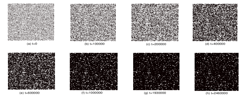
Figure 7: Evolution of agents on a $256\times 256$ lattice, with initial population of negative agents is a fraction $0.3$ of the total. ‘$-$’ agents are shown in black and ‘$+$’ agents in white. The data was collected over $50$ simulations and the final population of negative agents was $0.89-0.93$ of the total. This evolution is shown at different time steps for a representative simulation.

IV.2 B. Dynamics on a lattice

We now discuss the dynamics of the system on a lattice when $\beta$ is non-zero in eqn.(1). We take the same representative case when the initial population of ‘$-$’ agents is a fraction $0.3$ of the total and the final desired population of ‘$-$’ agents is a fraction $0.9$ of the total. For the simulation on a $256\times 256$ lattice, we have used $\beta=10.6$ and obtained a final population of ‘$-$’ agents between a fraction $0.89-0.93$ for $50$ simulations. We have chosen $\tau=10$, as a higher threshold has a slower effect in driving the system to an all ‘$-$’ population, compared to the simulations on completely connected networks. A representative simulation is shown in Fig. 7. Panel (a) shows the initial configuration with ‘$-$’ and ‘$+$’ agents $0.3$ and $0.7$ of the total population. Panel (b) shows the initial growth of the number of ‘$-$’ agents with the initial ‘$-$’ agents as seeds. The number of ‘$-$’ agents has grown significanltly even after $t=100000$ Monte Carlo steps. Panels (c) and (d) show the simulation at time steps $t=200000$ and $t=400000$ respectively and the growth of the clusters of ‘$-$’ agents is clearly visible. Panel (e) shows the simulation at $t=600000$ and the large clusters of ‘$-$’ agents have already emerged. These clusters further consolidate in panel (f) at $t=1000000$ and remain almost unchanged until the end of the simulation at $t=2469567$. This is easy to see from panels (f),(g) and (h).

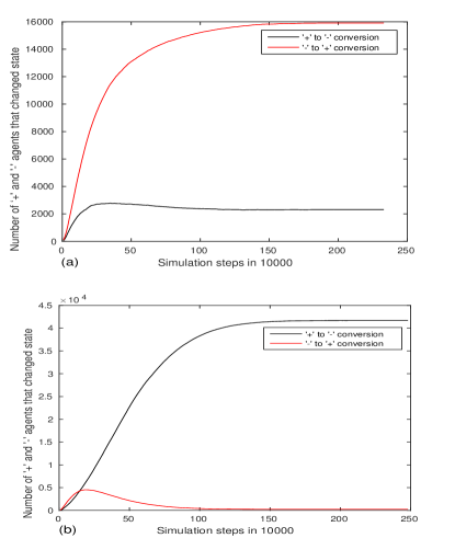
Figure 8: The conversion of agents from ‘$+$’ to ‘$-$’ and vice versa for a simulation on a $256\times 256$ lattice, with initial fraction of ‘$-$’ agents $0.3$, $p_{3}=0.9$ and $\tau=10$. (a) $\beta=0$, almost all ‘$-$’ agents are converted to ‘$+$’ (upper curve), compared to ‘$+$’ to ‘$-$’ conversions (lower curve); (b) $\beta=10.6$, the bias forces the conversion of a large number of ‘$+$’ agents to ‘$-$’ (upper curve) compared to ‘$-$’ to ‘$+$’ conversion (lower curve).

We show in Fig. 8 the conversion of agents from ‘$-$’ to ‘$+$’ and vice versa. The behavior is similar to the simulation on the lattice as the large-scale conversion of ‘$+$’ to ‘$-$’ agents occur quite early in the simulation. However, there is more conversion of ‘$-$’ agents to ‘$+$’ agents initially on the lattice compared to the completely connected network. The simulation takes a long time to complete since the agents reach their thresholds $\tau=10$ at the later stages of the simulation. The fractions of final population of ‘$-$’ agents for lattices of size $512\times 512$ and $1024\times 1024$ are within these bounds when $\beta=10.6$ and $\tau=10$ are used for the simulations. The partitions of $\theta^{+}$ values with $\tau=10$ and $\beta=10.6$ are $[0,1]_{[1-3]}$, $[1-2]_{[4-6]}$,$[2-3]_{[7-9]}$, $[3-4]_{[10]}$. It is evident that the dynamics of the system is dominated by the partitions $[0,1]_{[1-3]}$, $[1-2]_{[4-6]}$ as the conversions of ‘$+$’ to ‘$-$’ agents are rapid in the early stages of the simulation when the $\theta^{+}$ and $\theta^{-}$ counters of all agents have relatively lower values. This is similar to the simulations on the completely connected network.

initial population	$\beta$	target population	population achieved
0.1	3.0	0.6	0.59-0.64
0.1	5.2	0.7	0.68-0.73
0.2	1.8	0.6	0.59-0.64
0.2	3.0	0.7	0.65-0.77
0.4	1.2	0.7	0.68-0.73
0.4	2.8	0.8	0.76-0.83

Table 2: Simulation results on a lattice of $256\times 256$ agents. The result in each row is collected from $100$ simulations. The threshold is $\tau=10$ in all cases. The results were similar when simulations were run $10$ times each on lattices of size $512\times 512$ and $1024\times 1024$ agents.

Table 2 shows some more results from our simulations. We should note that it is possible to use higher values of $\tau$ for achieving sharper and more stable population fractions closer to the target population. We illustrate this in Fig. 9 with $0.3$ as the starting fraction of ‘$-$’ agents and $0.8$ as the target fraction. We vary $\tau$ for two fixed values of $\beta$. For $\beta=4.6$, the target fraction is reached at a lower value of $\tau=9$, however average target fraction was $0.82$ for $20$ simulations on a $256\times 256$ lattice. On the other hand a lower value of $\beta=2.3$ results in a slow convergence to the target fraction of $0.8$ at $\tau=25$, and the target fraction was $0.8$ every time for $20$ simulations. This behavior is common in our simulations, and its is possible to choose $\beta$ and $\tau$ pairs that allow us to achieve the target fraction accurately.

Fig. 9 has some similarities with rate-distortion curves studied in information theory CT . The aim of rate-distortion theory is to establish a connection between the channel capacity (rate) and output performance (distortion) of a communication channel, through minimizing channel distortion captured through a cost function. A rate-distortion curve separates the plane into two regions, allowable and non-allowable. The points in the allowable region indicate the minimum required rate to achieve a particular distortion in the output signal. Points in the non-allowable region indicate distortions that are unachievable using the corresponding rates. Two extreme points on a rate-distortion curve are the minimum rate required for zero distortion and the maximum distortion when the rate is zero. This also indicates a trade-off between the channel capacity and distortion, as distortion reduces by increasing channel capacity and increases by reducing channel capacity.

We can draw a parallel of Fig. 9 with a rate-distortion curve if we consider the interactions of agents in eqns. (1) and (2) as the channel capacity or rate, and the fraction $\phi$ as the output of the channel. Increasing $\tau$ increases the number of interactions between agents and can be seen as an increase in channel capacity. The distortion is the difference between the fraction $\phi$ achieved with a specific value of $\tau$ and the target fraction of ‘$-$’ agents. We can study a trade-off between $\tau$ and $\phi$ for a fixed $\beta$. For example, for $\beta=2.3$ (the red line marked with ‘x’ in Fig. 9), if we fix a value of $\tau$ and draw a vertical line, all the fractions $\phi$ of final population of ‘$-$’ agents below the red line are achievable with $\beta=2.3$. And no fraction $\phi$ above the red line is achievable with $\beta=2.3$. In other words, if we fix $\beta$, the red line divides the plane into allowable (below) and non-allowable (above) regions. A trade-off between $\tau$ and $\phi$ is also noticeable, as the non-allowable region is larger with smaller values of $\tau$ and vice versa. Similar trade-off due to rate-distortion curves has been observed in diverse domains like human perception S , capital asset pricing model for stocks O and balance between growth and entropy in bacterial cultures MCM .

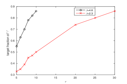
Figure 9: Slow and accurate convergence to the target fraction $0.8$ with different values of $\beta$ and $\tau$.

initial population	$\beta$	target population	achieved
0.1	$3.5\pm 2.0$	0.6	0.59-0.63
0.1	$5.5\pm 2.0$	0.7	0.69-0.73
0.2	$1.8\pm 1.1$	0.6	0.59-0.63
0.2	$3.0\pm 2.0$	0.7	0.69-0.73

Table 3: Simulation results on a completely connected network of $256\times 256$ agents. The result in each row is collected from $100$ simulations. The threshold is $\tau=5$ in all cases. The results were similar when simulations were run $10$ times each on completely connected networks of $512\times 512$ and $1024\times 1024$ agents.

IV.3 C. Dynamics with a faulty $\beta$

We have also experimented with the dynamics of the system when the bias $\beta$ is not constant for all the agents, rather $\beta$ varies within a range of values that we denote by $\beta\pm R$. We choose a value for $\beta$ from the range $\beta-R$ to $\beta+R$ uniformly at random at each Monte Carlo step for each agent. In other words, each agent uses a different $\beta$ within this range at each Monte Carlo step. Though the values of $\beta$ are different for achieving the desired fractions of final population of ‘$-$’ agents, the system is stable for a range of $\beta$ that is $\pm 2.0$ around a central value of $\beta$ for the cases when the central value of $\beta>2.0$. The deterioration in achieving the final desired fraction of ‘$-$’ agents starts beyond the $\pm 2.0$ range. Some results are shown in Table 3 for a completely connected network, and in Table 4 for lattices. The dynamics is quite similar in both cases. We have also verified that these results scale for larger networks.

initial population	$\beta$	target population	achieved
0.1	$3.2\pm 2.0$	0.6	0.59-0.63
0.1	$5.2\pm 2.0$	0.7	0.69-0.72
0.2	$3.0\pm 2.0$	0.7	0.69-0.73
0.4	$2.4\pm 2.0$	0.8	0.79-0.83

Table 4: Simulation results on a lattice of $256\times 256$ agents. The result in each row is collected from $100$ simulations. The threshold is $\tau=10$ in all cases. The results were similar when simulations were run $10$ times each on lattices of size $512\times 512$ and $1024\times 1024$ agents.

V V. Discussion

We have presented a model of opinion dynamics based on the negativity bias extensively studied in the psychology literature. Our main aim was to investigate the effect of negativity bias in binary opinion formation. One of the interesting aspects of our model is the formation of stable target population of ‘$-$’ agents. Our model is close to real-world exchange of opinions based on negativity bias. People with different opinions usually discuss pros and cons of both alternatives and gives more importance to negative opinions. We have abstracted this real-world situation in terms of the two counters for individual agents. We have shown that application of a power-law bias during opinion exchange results in consistent target populations and the bias factors are scale-invariant. Moreover, we have also shown that this consistency is maintained with bias factors that can vary randomly and uniformly within a range. Another interesting aspect of our model is its rapid convergence, the composition of the final population is reached quite early in the simulation, when each agent has interacted with only a few other agents. This is again close to the real-world situation in the sense that usually people even within a large population interact with a few other people while making decisions.

There are some similarities between the dynamics of our model and the dynamics of the random-field Ising model. For example, the conversions of ‘$+$’ to ‘$-$’ opinion and vice versa are similar to the first order phase transition in the random-field Ising model. Similarly, formation of clusters of ‘$+$’ and ‘$-$’ opinions and strong surface tension on cluster boundaries are very similar to the domains of similar spin in the random-field Ising model. We will explore these similarities further in future work.

VI acknowledgments

The author thankfully acknowledges very important suggestions from three referees who helped him to precisely define the scope of this work and improve its technical presentation.

References

- (1) P. Rozin and E. Royzman, Personality and Social Psychology Review, 5(4):296-320 (2001).
- (2) A. Vaish, T. Grossmann and A. Woodword, Psychological Bulletin, 134(3):383-403 (2008).
- (3) S. Galam, Int. J. Mod. Phys. C, 19, 409 (2008).
- (4) S. Galam, Physica A, 333, 453-460 (2004).
- (5) P. L. Krapivsky and S. Redner, Phys. Rev. Lett. 90, 238701 (2003).
- (6) T. M. Liggett, Annals of Probability 25, (1997).
- (7) T. M. Liggette, Interacting Particle Systems (Springer-Verlag, New York, 1985).
- (8) N. Lanchier and N. Taylor, Adv. in Appl. Probab., 47(3):668-692 (2015).
- (9) N. Crokidakis, J. Stat. Mech. (2009) P02058.
- (10) F. Schweitzer and L. Behera, European Physical Journal B: Condensed Matter and Complex Systems, 67 (3), 301-318 (2009).
- (11) P. Rozin and C. Nemeroff, in W. Stigler, R. A. Shweder and G. Hardt (Eds.) Cultural psychology: Essays on Comparative human development:205-232, Cambridge University Press (1990).
- (12) J. L. Cambier and M. Nauenberg, Phys. Rev. B 34(11):7998-8003 (1986).
- (13) C. Castellano, S. Fortunato, and V. Loreto, Rev. Mod. Phys. 81, 591 (2009).
- (14) N. Masuda, N. Gibert, and S. Redner, Phys. Rev. E 82, 010103(R) (2010).
- (15) N. Masuda, Phys. Rev. E 88, 052803 (2013).
- (16) C. Castellano, M.A. Muñoz, and R. Pastor-Satorras, Phys. Rev. E 80, 041129 (2009).
- (17) J. Binney, N. Dowrick, A. Fisher, and M. Newmann, The Theory of Critical Phenomena: An Introduction to the Renormalization Group (Oxford University Press, 1992).
- (18) D. Challet and Y-C. Zhang, Physica A 246, 407 (1997).
- (19) I. Dornic, H. Chaté, J. Chave, and H. Hinrichsen, Phys. Rev. Lett. 87(4):045701 (2001).
- (20) T. M. Cover and J. A. Thomas, Elements of Information Theory, 2nd. Edition, Wiley-Interscience (2006).
- (21) C. R. Sims, Cognition, 152:181-198 (2016).
- (22) W. D. O’Neill, Information Sciences, 83:55-74 (1995).
- (23) D. De Martino, F. Capuani and A. De Martino, Physical Biology, 13, 036005 (2016).