Revisit Batch Normalization: New Understanding from an Optimization View and a Refinement via Composition Optimization

Abstract

Batch Normalization (BN) has been used extensively in deep learning to achieve faster training process and better resulting models. However, whether BN works strongly depends on how the batches are constructed during training and it may not converge to a desired solution if the statistics on a batch are not close to the statistics over the whole dataset. In this paper, we try to understand BN from an optimization perspective by formulating the optimization problem which motivates BN. We show when BN works and when BN does not work by analyzing the optimization problem. We then propose a refinement of BN based on compositional optimization techniques called Full Normalization (FN) to alleviate the issues of BN when the batches are not constructed ideally. We provide convergence analysis for FN and empirically study its effectiveness to refine BN.

1 Introduction

Batch Normalization (BN) (Ioffe and Szegedy, 2015) has been used extensively in deep learning (Szegedy et al., 2016; He et al., 2016; Silver et al., 2017; Huang et al., 2017; Hubara et al., 2017) to accelerate the training process. During the training process, a BN layer normalizes its input by the mean and variance computed within a mini-batch. Many state-of-the-art deep learning models are based on BN such as ResNet (He et al., 2016; Xie et al., 2017) and Inception (Szegedy et al., 2016, 2017). It is often believed that BN can mitigate the exploding/vanishing gradients problem (Cooijmans et al., 2016) or reduce internal variance (Ioffe and Szegedy, 2015). Therefore, BN has become a standard tool that is implemented almost in all deep learning solvers such as Tensorflow (Abadi et al., 2015), MXnet (Chen et al., 2015), Pytorch (Paszke et al., 2017), etc.

Despite the great success of BN in quite a few scenarios, people with rich experiences with BN may also notice some issues with BN. Some examples are provided below.

BN fails/overfits when the mini-batch size is 1 as shown in Figure 1

We construct a simple network with 3 layers for a classification task. It fails to learn a reasonable classifier on a dataset with only 3 samples as seen in Figure 1.

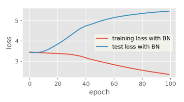
Figure 1: (Fail when batch size is 1) Given a dataset comprised of three samples: ${[}0,0,0{]}$ with label $0$, ${[}1,1,1{]}$ with label $1$ and ${[}2,2,2{]}$ with label $2$, use the following simple network including one batch normalization layer, where the numbers in the parenthesis are the dimensions of input and output of a layer: linear layer (3 $\rightarrow$3) $\Rightarrow$ batch normalization $\Rightarrow$ relu $\Rightarrow$ linear layer (3 $\rightarrow$ 3) $\Rightarrow$ nll loss.
Train with batch size 1, and test on the same dataset. The test loss increases while the training loss decreases.

BN’s solution is sensitive to the mini-batch size as shown in Figure 2

The test conducted in Figure 2 uses ResNet18 on the Cifar10 dataset. When the batch size changes, the neural network with BN training tends to converge to a different solution. Indeed, this observation is true even for solving convex optimization problems. It can also be observed that the smaller the batch size, the worse the performance of the solution.

BN fails if data are with large variation as shown in Figure 3

BN breaks convergence on simple convex logistic regression problems if the variance of the dataset is large. Figure 3 shows the first 20 epochs of such training on a synthesized dataset. This phenomenon also often appears when using distributed training algorithms where each worker only has its local dataset, and the local datasets are very different.

Therefore, these observations may remind people to ask some fundermental questions:

1. Does BN always converge and/or where does it converge to?

2. Using BN to train the model, why does sometimes severe over-fitting happen?

3. Why can BN often accelerate the training process?

4. Is BN a trustable “optimization” algorithm?

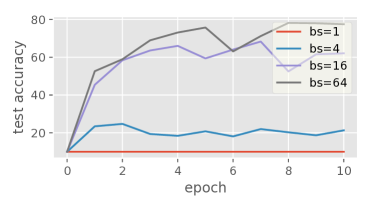
Figure 2: (Sensitive to the size of mini-batch) The test accuracy for ResNet18 on CIFAR10 dataset trained for 10 epochs with different batch sizes. The smaller the batch size is, with BN layers in ResNet, the worse the convergence result is.

In this paper, we aim at understanding the BN algorithm from a rigorous optimization perspective to show

1. BN always converges, but not solving either the objective in our common sense, or the optimization originally motivated.

2. The result of BN heavily depends on how to construct batches, and it can overfit predefined batches. BN treats the training and the inference differently, which makes the situation worse.

3. BN is not always trustable, especially when the batches are not constructed with randomly selected samples or the batch size is small.

Besides these, we also provide the explicit form of the original objective BN aims to optimize (but does not in fact), and propose a Multilayer Compositional Stochastic Gradient Descent (MCSGD) algorithm based on the compositional optimization technology to solve the original objective. We prove the convergence of the proposed MCSGD algorithm and empirically study its effectiveness to refine the state-of-the-art BN algorithm.

2 Related work

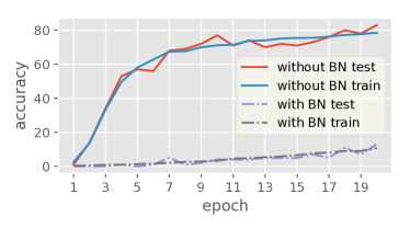
Figure 3: (Fail if data are with large variation) The training and test accuracy for a simple logistic regression problem on synthesized dataset with mini-batch size 20. We synthesize 10,000 samples where each sample is a vector of 1000 elements. There are 1000 classes. Each sample is generated from a zero vector by firstly randomly assigning a class to the sample (for example it is the $i$-th class), and then setting the $i$-th element of the vector to be a random number from 0 to 50, and finally adding noise (generated from a standard normal distribution) to each element. We generate 100 test samples in the same way. A logistic regression classifier should be able to classify this dataset easily. However, if we add a BN layer to the classifier, the model no longer converges.

We first review traditional normalization techniques. LeCun et al. (1998) showed that normalizing the input dataset makes training faster. In deep neural networks, normalization was used before the invention of BN. For example Local Response Normalization (LRU) (Lyu and Simoncelli, 2008; Jarrett K et al., 2009; Krizhevsky et al., 2012) which computes the statistics for the neighborhoods around each pixel.

We then review batch normalization techniques. Ioffe and Szegedy (2015) proposed the Batch Normalization (BN) algorithm which performs normalization along the batch dimension. It is more global than LRU and can be done in the middle of a neural network. Since during inference there is no “batch”, BN uses the running average of the statistics during training to perform inference, which introduces unwanted bias between training and testing. Ioffe (2017) proposed Batch Renormalization (BR) that introduces two extra parameters to reduce the drift of the estimation of mean and variance. However, Both BN and BR are based on the assumption that the statistics on a mini-batch approximates the statistics on the whole dataset.

Next we review the instance based normalization which normalizes the input sample-wise, instead of using the batch information. This includes Layer Normalization (Ba et al., 2016), Instance Normalization (Ulyanov et al., 2016), Weight Normalization (Salimans and Kingma, 2016) and a recently proposed Group Normalization (Wu and He, 2018). They all normalize on a single sample basis and are less global than BN. They avoid doing statistics on a batch, which work well when it comes to some vision tasks where the outputs of layers can be of handreds of channels, and doing statistics on the outputs of a single sample is enough. However we still prefer BN when it comes to the case that the single sample statistics is not enough and more global statistics is needed to increase accuracy.

Finally we review the compositional optimization which our refinement of BN is based on. Wang and Liu (2016) proposed the compositional optimization algorithm which optimizes the nested expectation problem $\min\mathbb{E}f(\mathbb{E}g(\cdot))$, and later the convergence rate was improved in Wang et al. (2016). The convergence of compositional optimization on nonsmooth regularized problems was shown in Huo et al. (2017) and a variance reduced variant solving strongly convex problems was analyzed in Lian et al. (2016).

3 Review the BN algorithm

In this section we review the Batch Normalization (BN) algorithm (Ioffe and Szegedy, 2015).

BN is usually implemented as an additional layer in neural networks. In each iteration of the training process, the BN layer normalizes its input using the mean and variance of each channel of the input batch to make its output having zero mean and unit variance. The mean and variance on the input batch is expected to be similar to the mean and variance over the whole dataset. In the inference process, the layer normalizes its input’s each channel using the saved mean and variance, which are the running averages of mean and variance calculated during training. This is described in Algorithm 1 and Algorithm 2. With BN, the input at the BN layer is normalized so that the next layer in the network accepts inputs that are easier to train on. In practice it has been observed in many applications that the speed of training is improved by using BN.

Algorithm 1 Batch Normalization Layer (Training)

1:Input $\mathbf{B}_{\text{in}}$, which is a batch of input. Estimated mean $\mu$ and variance $\nu$, and averaging constant $\alpha$.

2:

$$\mu\leftarrow (1-\alpha)\cdot\mu+\alpha\cdot\textbf{{mean}}(\mathbf{B}_{\text{in}}),$$

$$\nu\leftarrow (1-\alpha)\cdot\nu+\alpha\cdot\textbf{{var}}(\mathbf{B}_{\text{in}}).$$

$\triangleright$ $\textbf{{mean}}(\mathbf{B}_{\text{in}})$ and $\textbf{{var}}(\mathbf{B}_{\text{in}})$ calculate the mean and variance of $\mathbf{B}_{\text{in}}$ respectively.

3:Output

$$\mathbf{B}_{\text{out}}\leftarrow\frac{\mathbf{B}_{\text{in}}-\textbf{{mean}}(\mathbf{B}_{\text{in}})}{\sqrt{\textbf{{var}}(\mathbf{B}_{\text{in}})+\epsilon}}.$$

$\triangleright$ $\epsilon$ is a small constant for numerical stability.

Algorithm 2 Batch Normalization Layer (Inference)

1:Input $\mathbf{B}_{\text{in}}$, estimated mean $\mu$ and variance $\nu$. A small constant $\epsilon$ for numerical stability.

2:Output

$$\mathbf{B}_{\text{out}}\leftarrow\frac{\mathbf{B}_{\text{in}}-\mu}{\sqrt{\nu+\epsilon}}.$$

4 Training objective of BN

In the original paper proposing BN algorithm (Ioffe and Szegedy, 2015), authors do not provide the explicit optimization objective BN targets to solve. Therefore, many people may naturally think that BN is an optimization trick, that accelerates the training process but still solves the original objective in our common sense. Unfortunately, this is not true! The actual objective BN solves is different from the objective in our common sense and also nontrivial.

Rigorous mathematical description of BN layer

To define the objective of BN in a precise way, we need to define the normalization operator $f^{B,\sigma}_{W}$ that maps a function to a function associating with a mini-batches $B$, an activation function $\sigma$, and parameters $W$. Let $g(\cdot)$ be a function

$$g(\cdot)=\left(\begin{matrix}g_{1}(\cdot)\\ g_{2}(\cdot)\\ \cdots\\ g_{n}(\cdot)\\ 1\end{matrix}\right)$$

where $g_{1}(\cdot),\cdots,g_{n}(\cdot)$ are functions mapping a vector to a number. The operator $f^{B,\sigma}_{W}$ is defined by

$$\underbrace{f^{B,\sigma}_{W}\overbrace{(g)}^{\mathclap{\begin{subarray}{c}\text{$f_{W}^{B,\sigma}$'s argument is}\\ \text{a function $g$}\end{subarray}}}}_{\mathclap{\begin{subarray}{c}\text{$f_{W}^{B,\sigma}(g)$ is}\\ \text{another function}\end{subarray}}}(\cdot):=\sigma\left(W\left(\begin{array}[]{c}\frac{g_{1}(\cdot)-\textbf{mean}(g_{1},B)}{\sqrt{\textbf{var}(g_{1},B)}}\\ \frac{g_{2}(\cdot)-\textbf{mean}(g_{2},B)}{\sqrt{\textbf{var}(g_{2},B)}}\\ \vdots\\ \frac{g_{n}(\cdot)-\textbf{mean}(g_{n},B)}{\sqrt{\textbf{var}(g_{n},B)}}\\ 1\end{array}\right)\right)$$ (6)

where $\textbf{mean}(r,B)$ is defined by

$$\textbf{mean}(r,B):=\frac{1}{|B|}\sum_{b\in B}r(b).$$

and $\textbf{var}(r,B)$ is defined by

$$\textbf{var}(r,B)=\textbf{mean}(r^{2},B)-\textbf{mean}(r,B)^{2}.$$

Note that the first augment of $\textbf{mean}(\cdot,\cdot)$ and $\textbf{var}(\cdot,\cdot)$ is a function, and the second augment is a set of samples. A $m$-layer’s neural network with BN can be represented by a function

$$F^{B}_{\{W_{i}\}_{i=1}^{m}}(\cdot):=f_{W_{m}}^{B,\sigma_{m}}(f_{W_{m-1}}^{B,\sigma_{m-1}}(\cdots(f_{W_{1}}^{B,\sigma_{1}}(I))))(\cdot)\quad\text{or}\quad f_{W_{m}}^{B,\sigma_{m}}\circ f_{W_{m-1}}^{B,\sigma_{m-1}}\circ\cdots\circ f_{W_{1}}^{B,\sigma_{1}}(I)(\cdot)$$

where $I(\cdot)$ is the identical mapping function from a vector to itself, that is, $I(x)=x$.

BN’s objective is very different from the objective in our common sense

Using the same way, we can represent a fully connected network in our common sense (without BN) by

$$F_{\{W_{i}\}_{i=1}^{m}}(\cdot):=\bar{f}_{W_{m}}^{\sigma_{m}}\circ\bar{f}_{W_{m-1}}^{\sigma_{m-1}}\circ\cdots\circ\bar{f}_{W_{1}}^{\sigma_{1}}(I)(\cdot)$$

where operator $\bar{f}_{W}^{\sigma}$ is defined by

$$\bar{f}^{\sigma}_{W}(g)(\cdot):=\sigma(Wg(\cdot)).$$ (7)

Besides of the difference of operator function definitions, their ultimate objectives are also different. Given the training date set $\mathcal{D}$, the objective without BN (or the objective in our common sense) is defined by

$$\min_{\{W_{j}\}_{j=1}^{m}}\quad{1\over|\mathcal{D}|}\sum_{({\bf{x}},y)\in\mathcal{D}}l(F_{\{W_{j}\}_{j=1}^{m}}({\bf{x}}),y),$$ (8)

where $l(\cdot,\cdot)$ is a predefined loss function, while the objective with BN (or the objective BN is actually solving) is

$$({\bf BN})\quad\min_{\{W_{j}\}_{j=1}^{m}}\quad{1\over|\mathcal{B}|}\sum_{B\in\mathcal{B}}{1\over|B|}\sum_{({\bf{x}},y)\in B}l(F^{B}_{\{W_{j}\}_{j=1}^{m}}({\bf{x}}),y),$$ (9)

where $\mathcal{B}$ is the set of batches.

Therefore, the objective of BN could be very different from the objective in our common sense in general.

BN could be very sensitive to the sample strategy and the minibatch size

The super set $\mathcal{B}$ has different forms depending on how to define mini-batchs. For example,

• People can choose $b$ as the size of minibatch, and form $\mathcal{B}$ by

  $$\mathcal{B}:=\left\{B\subset\mathcal{D}:~{}|B|=b\right\}.$$

  Choosing $\mathcal{B}$ in this way implicitly assumes that all nodes can access the same dataset, which may not be true in practice.

• If data is distributed ($\mathcal{D}_{i}$ is the local dataset on the $i$-th worker, disjoint with others, satisfying $\mathcal{D}=\mathcal{D}_{1}\cup\cdots\cup\mathcal{D}_{n}$), a typical $\mathcal{B}$ is defined by $\mathcal{B}=\mathcal{B}_{1}\cup\mathcal{B}_{2}\cup\cdots\cup\mathcal{B}_{n}$ with $\mathcal{B}_{i}$ defined by

  $$\mathcal{B}_{i}:=\left\{B\subset\mathcal{D}_{i}:~{}|B|=b\right\}.$$

• When the mini-batch is chosen to be the whole dataset, $\mathcal{B}$ contains only one element $\mathcal{D}$.

After figure out the implicit objective BN optimizes in (9), it is not difficult to have following key observations

• The BN objectives vary a lot when different sampling strategies are applied. This explains why the convergent solution could be very different when we change the sampling strategy;

• For the same sample strategy, BN’s objective function also varies if the size of minibatch gets changed. This explains why BN could be sensitive to the batch size.

The observations above may seriously bother us how to appropriately choose parameters for BN, since it does not optimize the objective in our common sense, and could be sensitive to the sampling strategy and the size of minibatch.

BN’s objective (9) with $\mathcal{B}=\{\mathcal{D}\}$ has the same optimal value as the original objective (8)

When the batch size is equal to the size of the whole dataset in (9), the objective becomes

$$(\textbf{FN})\quad\min_{\{W_{j}\}_{j=1}^{m}}\quad{1\over|\mathcal{D}|}\sum_{({\bf{x}},y)\in\mathcal{D}}l(F^{\mathcal{D}}_{\{W_{j}\}_{j=1}^{m}}({\bf{x}}),y),$$ (10)

which differs from the original objective (8) only in the first argument of $l$. Noting the only difference between (6) and (7) when $B$ is a constant $\mathcal{D}$ is a linear transformation which can be absorbed into $W$:

$$f^{\mathcal{D},\sigma}_{W}(g)(\cdot)=\sigma\left(W\left(\begin{array}[]{c}\frac{g_{1}(\cdot)-\textbf{mean}(g_{1},\mathcal{D})}{\sqrt{\textbf{var}(g_{1},\mathcal{D})}}\\ \frac{g_{2}(\cdot)-\textbf{mean}(g_{2},\mathcal{D})}{\sqrt{\textbf{var}(g_{2},\mathcal{D})}}\\ \vdots\\ \frac{g_{n}(\cdot)-\textbf{mean}(g_{n},\mathcal{D})}{\sqrt{\textbf{var}(g_{n},\mathcal{D})}}\\ 1\end{array}\right)\right)$$

$$= \sigma\left(\underbrace{W\scriptsize{\left(\begin{array}[]{ccccc}\frac{1}{\sqrt{\textbf{var}(g_{1},\mathcal{D})}}&&&&\frac{-\textbf{mean}(g_{1},\mathcal{D})}{\sqrt{\textbf{var}(g_{1},\mathcal{D})}}\\ &\frac{1}{\sqrt{\textbf{var}(g_{2},\mathcal{D})}}&&&\frac{-\textbf{mean}(g_{2},\mathcal{D})}{\sqrt{\textbf{var}(g_{2},\mathcal{D})}}\\ &&\ddots&&\vdots\\ &&&\frac{1}{\sqrt{\textbf{var}(g_{n},\mathcal{D})}}&\frac{-\textbf{mean}(g_{n},\mathcal{D})}{\sqrt{\textbf{var}(g_{n},\mathcal{D})}}\\ &&&&1\end{array}\right)}}_{=:W^{\prime}}\left(\begin{array}[]{c}g_{1}(\cdot)\\ g_{2}(\cdot)\\ \vdots\\ g_{n}(\cdot)\\ 1\end{array}\right)\right)$$

$$= \sigma\left(W^{\prime}\left(\begin{array}[]{ccccc}g_{1}(\cdot)&g_{2}(\cdot)&\cdots&g_{n}(\cdot)&1\end{array}\right)^{\top}\right).$$

If we use this $W^{\prime}$ as our new $W$, (8) and (9) has the same form and the two objectives should have the same optimal value, which means when $\mathcal{B}=\{\mathcal{D}\}$ adding BN does not hurt the expressiveness of the network. However, since each layer’s input has been normalized, in general the condition number of the objective is reduced, and thus easier to train.

5 Solving full normalization objective (10) via compositional optimization

The BN objective contains the normalization operator which mostly reduces the condition number of the objective that can accelerate the training process. While the FN formulation in (10) provides a more stable and trustable way to define the BN formation, it is very challenging to solve the FN formulation in practice. If follow the standard SGD used in solving BN to solve (10), then every single iteration needs to involve the whole dataset since $B=\mathcal{D}$, which is almost impossible in practice. The key difficulty to solve (10) lies on that there exists “expectation” in each layer, which is very expensive to compute even we just need to compute a stochastic gradient if use the standard SGD method.

To solve (10) efficiently, we follow the spirit of compositional optimization to develop a new algorithm namely, Multilayer Compositional Stochastic Gradient Descent (Algorithm 3). The proposed algorithm does not have any requirement on the size of minibatch. The key idea is to estimate the expectation from the current samples and historical record.

5.1 Formulation

To propose our solution to solve (10), let us define the objective in a more general but neater way in the following.

When $\mathcal{B}=\{\mathcal{D}\}$, (9) is a special case of the following general objective:

$$\min_{w}f(w):= \mathbb{E}_{\xi}\Big{[}F_{1}^{w_{1},\mathcal{D}}\circ F_{2}^{w_{2},\mathcal{D}}\circ\cdots\circ F_{n}^{w_{n},\mathcal{D}}\circ I(\xi)\Big{]},$$ (11)

where $\xi$ represents a sample in the dataset $\mathcal{D}$, for example it can be the pair $({\bf{x}},y)$ in (9). $w_{i}$ represents the parameters of the $i$-th layer. $w$ represents all parameters of the layers: $w:=(w_{1},\ldots,w_{n})$. Each $F_{i}$ is an operator of the form:

$$F_{i}^{w_{i},\mathcal{D}}(g)(\cdot):= F_{i}(w_{i};g(\cdot);\mathbb{E}_{\xi\in\mathcal{D}}e_{i}(g(\xi))),$$

where $e_{i}$ is used to compute statistics over the dataset. For example, with $e_{i}(x)=[x,x^{2}]$, the mean and variance of the layer’s input over the dataset can be calculated, and $F_{i}^{w_{i},\mathcal{D}}$ can use that information, for example, to perform normalization.

There exist compositional optimization algorithms (Wang and Liu, 2016; Wang et al., 2016) for solving (11) when $n=2$, but for $n>2$ we still do not have a good algorithm to solve it. We follow the spirit to extend the compositional optimization algorithms to solve the general optimization problem (11) as shown in Algorithm 3. See Section 6 for an implementation when it comes to normalization.

To simplify notation, given $w=(w_{1},\ldots,w_{n})$ we define:

$$\mathbf{e}_{i}(w;\xi):= e_{i}({F}_{i+1}^{w_{i+1},\mathcal{D}}\circ{F}_{i+2}^{w_{i+2},\mathcal{D}}\circ\cdots\circ{F}_{n}^{w_{n},\mathcal{D}}\circ I(\xi)).$$

We define the following operator if we already have an estimation, say $\hat{e}_{i}$, of $\mathbb{E}_{\xi\in\mathcal{D}}\mathbf{e}_{i}(w;\xi)$:

$$\hat{F}_{i}^{w_{i},\hat{e}_{i}}(g)(\cdot):= F_{i}(w_{i};g(\cdot);\hat{e}_{i}).$$

Given $w=(w_{1},\ldots,w_{n})$ and $\hat{e}=(\hat{e}_{1},\ldots,\hat{e}_{n})$, we define

$$\hat{\mathbf{e}}_{i}(w;\xi;\hat{e}):= e_{i}(\hat{F}_{i+1}^{w_{i+1},\hat{e}_{i+1}}\circ\hat{F}_{i+2}^{w_{i+2},\hat{e}_{i+2}}\circ\cdots\circ\hat{F}_{n}^{w_{n},\hat{e}_{n}}\circ I(\xi)).$$

Algorithm 3 Multilayer Compositional Stochastic Gradient Descent (MCSGD) algorithm

1:Learning rate $\{\gamma_{k}\}_{k=0}^{K}$, approximation rate $\{\alpha_{k}\}_{k=0}^{K}$, dataset $\mathcal{D}$, initial point $w^{(0)}:=(w_{1}^{(0)},\ldots,w_{n}^{(0)})$ and initial estimations $\hat{e}^{(0)}:=(\hat{e}_{1}^{(0)},\ldots,\hat{e}_{n}^{(0)})$.

2:for $k=0,1,2,\ldots,K$ do

3:     For each $i$, randomly select a sample $\xi_{k}$, estimate $\mathbb{E}_{\xi}[\mathbf{e}_{i}(w^{(k)};\xi)]$ by

$$\hat{e}_{i}^{(k+1)}\leftarrow(1-\alpha_{k})\hat{e}_{i}^{(k)}+\alpha_{k}\hat{\mathbf{e}}_{i}(w^{(k)};\xi_{k};\hat{e}^{(k)}).$$

4:     Ask the oracle $\mathcal{O}$ using $w^{(k)}$ and estimated means $\hat{e}^{(k+1)}$ to obtain the approximated gradient at $w^{(k)}$: $g^{(k)}$. $\triangleright$ See Remark 1 for discussion on the oracle.

5:     $w^{(k+1)}\leftarrow w^{(k)}-\gamma_{k}g^{(k)}$.

6:end for

Remark 1 (MCSGD oracle).

In MCSGD, the gradient oracle takes the current parameters of the model, and the current estimation of each $\mathbb{E}_{\xi}[\mathbf{e}_{i}(w^{(k)};\xi)]$, to output an estimation of a stochastic gradient.

For example for an objective like (11), the derivative of the loss function w.r.t. the $i$-th layer’s parameters is

$$\partial_{w_{i}}f(w)= \partial_{w_{i}}(\mathbb{E}_{\xi}[F_{1}^{w_{1},\mathcal{D}}\circ F_{2}^{w_{2},\mathcal{D}}\circ\cdots\circ F_{n}^{w_{n},\mathcal{D}}\circ I(\xi)])$$

$$= \mathbb{E}_{\xi}\left[\begin{array}[]{l}{}[\partial_{x}(F_{1}^{w_{1},\mathcal{D}}(x)(\xi))]_{x=F_{2}^{w_{2},\mathcal{D}}\circ\cdots\circ F_{n}^{w_{n},\mathcal{D}}\circ I}\cdot\\ {}[\partial_{x}(F_{2}^{w_{2},\mathcal{D}}(x)(\xi))]_{x=F_{3}^{w_{3},\mathcal{D}}\circ\cdots\circ F_{n}^{w_{n},\mathcal{D}}\circ I}\cdot\cdots\cdot\\ {}[\partial_{x}(F_{i-1}^{w_{i-1},\mathcal{D}}(x)(\xi))]_{x=F_{i}^{w_{i},\mathcal{D}}\circ\cdots\circ F_{n}^{w_{n},\mathcal{D}}\circ I}\cdot\\ {}[\partial_{w_{i}}(F_{i}^{w_{i},\mathcal{D}}(x)(\xi))]_{x=F_{i}^{w_{i+1},\mathcal{D}}\circ\cdots\circ F_{n}^{w_{n},\mathcal{D}}\circ I}\end{array}\right],$$ (12)

where for any $j\in[1,\ldots,i-1]$:

$${}[\partial_{x}F_{j}^{w_{j},\mathcal{D}}(x)(\xi)]_{x=F_{j+1}^{w_{j+1},\mathcal{D}}\circ\cdots\circ F_{n}^{w_{n},\mathcal{D}}\circ I}= \left[\begin{array}[]{c}\partial_{x}F_{j}(w_{j};x;y)+\\ \partial_{y}F_{j}(w_{j};x;y)\cdot\mathbb{E}_{\xi^{\prime}\sim\mathcal{D}}D_{j}(\xi^{\prime})\end{array}\right]$$

$$\text{with}\left\{\begin{array}[]{l}x=F_{j+1}^{w_{j+1},\mathcal{D}}\circ\cdots\circ F_{n}^{w_{n},\mathcal{D}}\circ I(\xi)\\ y=\mathbb{E}_{\xi}[\mathbf{e}_{j}(w;\xi)]\\ D_{j}(\xi^{\prime})=[\partial_{z}e_{i}(z)]_{z=F_{j+1}^{w_{j+1},\mathcal{D}}\circ\cdots\circ F_{n}^{w_{n},\mathcal{D}}\circ I(\xi^{\prime})}\end{array}\right..$$

The oracle samples a $\xi^{\prime}$ for each layer and calculate this derivative with $y$ set to an estimated value $\hat{e}_{j}$, and returns the stochastic gradient. The expectation of this stochastic gradient will be (12) with some error caused by the difference between the estimated $\hat{e}_{j}$ and the true expectation $\mathbb{E}_{\xi}[\mathbf{e}_{j}(w;\xi)]$. The more accurate the estimation is, the closer the expectation of this stochastic and the true gradient (12) will be.

In practice, we often use the same $\xi^{\prime}$ for each layer to save some computation resource, this introduce some bias the expectation of the estimated stochastic gradient. One such implementation can be found in Algorithm 4.

5.2 Theoretical analysis

In this section we analyze Algorithm 3 to show its convergence when applied on (11) (a generic version of the FN formulation in (10)). The detailed proof is provided in the supplementary material. We use the following assumptions as shown in 1 for the analysis.

Assumption 1.

1. The gradients $g^{(k)}$’s are bounded:

   $$\|g^{(k)}\|\leqslant\mathscr{G},\forall k$$

   for some constant $\mathscr{G}$.

2. The variance of all $e_{i}$’s are bounded:

   $$\mathbb{E}_{\xi}\|\mathbf{e}_{i}(w;\xi)-\mathbb{E}_{\xi}\mathbf{e}_{i}(w;\xi)\|^{2}\leqslant\sigma^{2},\forall i,w,$$

   $$\mathbb{E}_{\xi}\|\mathbf{e}_{i}(w;\xi;\hat{e})-\mathbb{E}_{\xi}\mathbf{e}_{i}(w;\xi;\hat{e})\|^{2}\leqslant\sigma^{2},\forall i,w,\hat{e}$$

   for some constant $\sigma$.

3. The error of approximated gradient $\mathbb{E}[g^{(k)}]$ is proportional to the error of approximation for $\mathbb{E}[e_{i}]$:

   $$\|\mathbb{E}_{\xi_{k}}[g^{(k)}]-\nabla f(w^{(k)})\|^{2}\leqslant L_{g}\sum_{i=1}^{n}\|\hat{e}_{i}^{(k+1)}-\mathbb{E}_{\xi_{k}}[\mathbf{e}_{i}(w^{(k)};\xi_{k})]\|^{2},\forall k$$

   for some constant $L_{g}$.

4. All functions and their first order derivatives are Lipschitzian with Lipschitz constant $L$.

5. The minimum of the objective $f(w)$ is finite.

6. $\gamma_{k},\alpha_{k}$ are monotonically decreasing. $\gamma_{k}=O(k^{-\gamma})$ and $\alpha_{k}=O(k^{-a})$ for some constants $\gamma>a>0$.

It can be shown under the given assumptions, the approximation errors will vanish shown in Lemma 1.

Lemma 1 (Approximation error).

Choose the learning rate $\gamma_{k}$ and $\alpha_{k}$ in Algorithm 3 in the form defined in Assumption 1-6 with parameters $\gamma$ and $a$. Under 1, the sequence generated in Algorithm 3 satisfies

$$\mathbb{E}\|\hat{e}_{i}^{(k+1)}-\mathbb{E}_{\xi}\mathbf{e}_{i}(w^{(k)};\xi)\|^{2}\leqslant \mathscr{E}(k^{-2\gamma+2a+\varepsilon}+k^{-a+\varepsilon}),\forall i,\forall k.$$ (13)

$$\mathbb{E}\|\hat{e}_{i}^{(k+1)}-\mathbb{E}_{\xi}\mathbf{e}_{i}(w^{(k)};\xi)\|^{2}\leqslant \left(1-\frac{\alpha_{k}}{2}\right)\mathbb{E}\|\hat{e}_{i}^{(k)}-\mathbb{E}_{\xi}\mathbf{e}_{i}(w^{(k-1)};\xi)\|^{2}$$

$$+\mathscr{C}(k^{-2\gamma+a+\varepsilon}+k^{-2a+\varepsilon}),\quad\forall i,\forall k.$$ (14)

for any $\varepsilon$ satisfying $1-a>\varepsilon>0$, where $\mathscr{E}$ and $\mathscr{C}$ are two constants independent of $k$.

Then it can be shown that on (11) Algorithm 3 converges as seen in Theorem 2 and Corollary 3. It is worth noting that the convergence rate in Corollary 3 is slower than the $\frac{1}{\sqrt{K}}$ convergence rate of SGD without any normalization. This is due to the estimation error. If the estimation error is small (for example, the samples in a batch are randomly selected and the batch size is large), the convergence will be fast.

Theorem 2 (Convergence).

Choose the learning rate $\gamma_{k}$ and $\alpha_{k}$ in Algorithm 3 in the form defined in Assumption 1-6 with parameters $\gamma$ and $a$ satisfying $a<2\gamma-1,a<1/2$, and $\frac{\gamma_{k}L_{g}}{\alpha_{k+1}}\leqslant\frac{1}{2}$. Under 1, for any integer $K>1$ the sequence generated by Algorithm 3 satisfies

$$\frac{\sum_{k=0}^{K}\gamma_{k}\mathbb{E}\|\partial f(w^{(k)})\|^{2}}{\sum_{k=0}^{K}\gamma_{k}}\leqslant \frac{\mathscr{H}}{\sum_{k=0}^{K}\gamma_{k}},$$

where $\mathscr{H}$ is a constant independent of $K$.

We next specify the choice of $\gamma$ and $a$ to give a more clear convergence rate for our MCSGD algorithm in Corollary 3.

Corollary 3.

Choose the learning rate $\gamma_{k}$ and $\alpha_{k}$ in Algorithm 3 in the form defined in Assumption 1-6, more specifically, $\gamma_{k}=\frac{1}{2L_{g}}(k+2)^{-4/5}$ and $\alpha_{k}=(k+1)^{-2/5}$. Under 1, for any integer $K>1$ the sequence generated in Algorithm 3 satisfies

$$\frac{\sum_{k=0}^{K}\mathbb{E}\|\partial f(w^{(k)})\|^{2}}{K+2}\leqslant\frac{\mathscr{H}}{(K+2)^{1/5}},$$

where $\mathscr{H}$ is a constant independent of $K$.

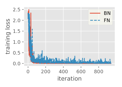
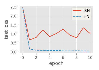
Figure 4: The training and testing error for the given model trained on MNIST with batch size 64, learning rate 0.01 and momentum 0.5 using BN or FN for the case where all samples in a batch are of a single label. The approximation rate $\alpha$ in FN is $(\frac{k}{20}+1)^{-0.4}$ where $k$ is the iteration number.

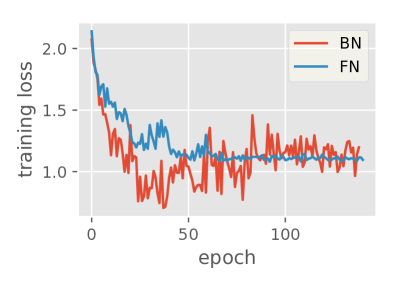
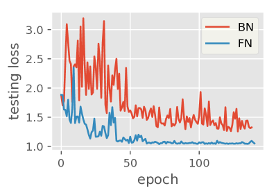
Figure 5: The training and testing error for the given model trained on CIFAR10 with batch size 64, learning rate 0.01 and momentum 0.9 using BN and FN for the case where all samples in a batch are of no more than 3 labels. The learning rate is decreased by a factor of 5 for every 20 epochs. The approximation rate $\alpha$ in FN is $(\frac{k}{5}+1)^{-0.3}$ where $k$ is the iteration number.

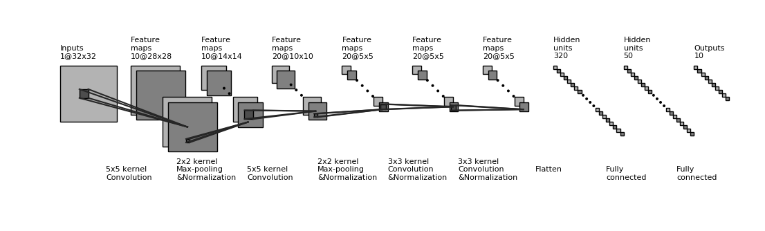
Figure 6: The simple neural network used in the experiments. The “Normalization” between layers can be BN or FN. The activation function is relu and the loss function is negative log likelihood.

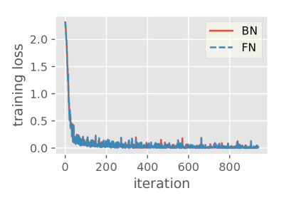
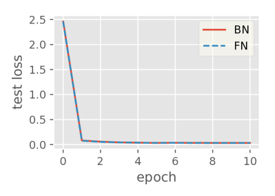
Figure 7: The training and testing error for the given model trained on MNIST with batch size 64, learning rate 0.01 and momentum 0.5 using BN or FN for the case where samples in a batch are randomly selected. The approximation rate $\alpha$ in FN is $(\frac{k}{20}+1)^{-0.4}$ where $k$ is the iteration number.

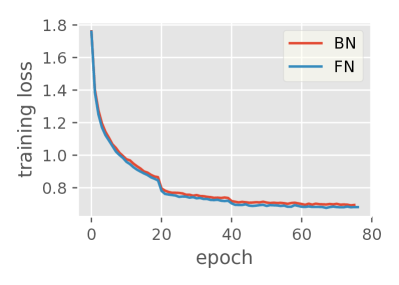
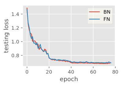
Figure 8: The training and testing error for the given model trained on CIFAR10 with batch size 64, learning rate 0.01 and momentum 0.9 using BN or FN for the case where samples in a batch are randomly selected. The learning rate is decreased by a factor of 5 for every 20 epochs. The approximation rate $\alpha$ in FN is $(\frac{k}{20}+1)^{-0.2}$ where $k$ is the iteration number.

6 Experiments

Experiments are conducted to validate the effectiveness of our MCSGD algorithm for solving the FN formulation. We consider two settings. The first one in Section 6.1 shows BN’s convergence highly depends on the size of batches, while FN is more robust to different batch sizes. The second one in Section 6.2 shows that FN is more robust to different construction of mini-batches.

We use a simple neural network as the testing network whose architecture is shown in Figure 6. Steps 2 and 3 in Algorithm 3 are implemented in Algorithm 4. The forward pass essentially performs Step 2 of Algorithm 3, which estimates the mean and variance of layer inputs over the dataset. The backward pass essentially performs Step 3 of Algorithm 3, which gives the approximated gradient based on current network parameters and the estimations. Note that as discussed in Remark 1, for efficiency, in each iteration of this implementation we are using the same samples to do estimation in all normalization layers, which saves computational cost but brings additional bias.

Algorithm 4 Full Normalization (FN) layer

Forward pass

1:Learning rate $\gamma$, approximation rate $\alpha$, input $\mathbf{B}_{\text{in}}\in\mathbb{R}^{b\times d}$, mean estimation $\mu$, and mean of square estimation $\nu$. $\triangleright$ $b$ is the batch size, and $d$ is the dimension of each sample.

2:if training then

$$\mu\leftarrow (1-\alpha)\mu+\alpha\textbf{{mean}}(\mathbf{B}_{\text{in}}),$$

$$\nu\leftarrow (1-\alpha)\nu+\alpha\textbf{{mean\_of\_square}}(\mathbf{B}_{\text{in}}).$$

3:end if

4:return layer output:

$$\mathbf{B}_{\text{output}}\leftarrow\frac{\mathbf{B}_{\text{in}}-\mu}{\sqrt{\max\{\nu-\mu^{2},\epsilon\}}}.$$

$\triangleright$ $\epsilon$ is a small constant for numerical stability.

Backward pass

1:Mean estimation $\mu$, mean of square estimation $\nu$, the gradient at the output $g_{\text{out}}$, and input $\mathbf{B}_{\text{in}}\in\mathbb{R}^{b\times d}$.

2:Define

$$f(\mu,\nu,\mathbf{B}_{\text{in}}):=\frac{\mathbf{B}_{\text{in}}-\mu}{\sqrt{\max\{\nu-\mu^{2},\epsilon\}}}.$$

3:return the gradient at the input:

$$g_{\text{in}}\leftarrow g_{\text{out}}\cdot\left(\partial_{\mathbf{B}_{\text{in}}}f+\frac{\partial_{\mu}f+2\mathbf{B}_{\text{in}}\partial_{\nu}f}{bd}\right).$$

$\triangleright$ $\partial_{a}f$ is the derivative of $f$ w.r.t. $a$ at $\mu,\nu,\mathbf{B}_{\text{in}}$.

6.1 Dependence on batch size

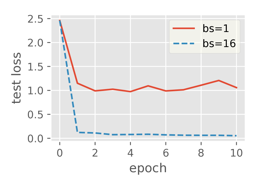
(a) With BN layers.

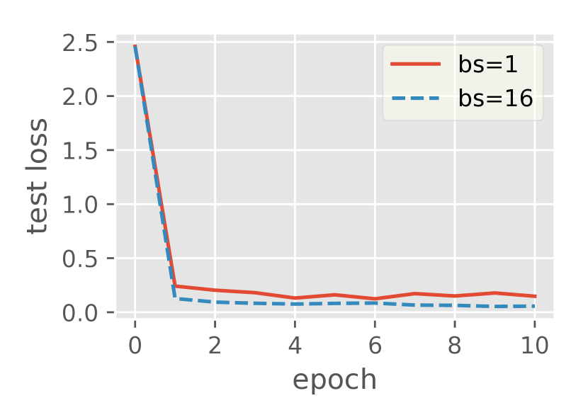
(b) With FN layers.

Figure 9: The testing error for the given model trained on MNIST, where each sample is multiplied by a random number in $(-2.5,2.5)$. The optimization algorithm is SGD with learning rate is 0.01 and momentum is 0.5. FN gives more consistent results under different batch sizes. The approximation rate $\alpha$ in FN is $(\frac{k}{20}+1)^{-0.4}$ where $k$ is the iteration number.

MNIST is used as the testing dataset with some modification by multiplying a random number in $(-2.5,2.5)$ to each sample to make them more diverse. In this case, as shown in Figure 9, with batch size 1 and batch size 16, we can see the convergent points are different in BN, while the convergent results of FN are much more close for different batch sizes. Therefore, FN is more robust to the size of mini-batch.

6.2 Dependence on batch construction

We study two cases — shuffled case and unshuffled case. For the shuffled case, where the samples in a batch are randomly sampled, we expect the performance of FN matches BN’s in this case. For the unshuffled case, where the batch contains only samples in just a few number of categories (so the mean and variance are very different from batch to batch). In this case we can observe that the FN outperforms BN.

Unshuffled case

We show the FN has advantages over BN when the data variation is large among mini-batches. In the unshuffled setting, we do not shuffle the dataset. It means that the samples in the same mini-batch are mostly with the same labels. The comparison uses two datasets (MINST and CIFAR10):

• On MNIST, the batch size is chosen to be 64 and each batch only contains a single label. The convergence results are shown in Figure 4. We can observe from these figures that for the training loss, BN and FN converge equally fast (BN might be slightly faster). However since the statistics on any batch are very different from the whole dataset, the estimated mean and variance in BN are very different from the true mean and variance on the whole dataset, resulting in a very high test loss for BN.

• On CIFAR10, we observe similar results as shown in Figure 5. In this case, we restrict the number of labels in every batch to be no more than 3. Thus BN’s performance on CIFAR10 is slightly better than on MNIST. We see the convergence efficiency of both methods is still comparable in term of the training loss. However, the testing error for BN is still far behind the FN.

Shuffled case

For the shuffled case, where the samples in each batch are selected randomly, we expect BN to have similar performance as FN in this case, since the statistics in a batch is close to the statistics on the whole dataset. The results for MNIST are shown in Figure 7 and the results for CIFAR10 are shown in Figure 8. We observe the convergence curves of BN and FN for both training and testing loss match well.

7 Conclusion

We provide new understanding for BN from an optimization perspective by rigorously defining the optimization objective for BN. BN essentially optimizes an objective different from the one in our common sense. The implicitly targeted objective by BN depends on the sampling strategy as well as the minibatch size. That explains why BN becomes unstable and sensitive in some scenarios. The stablest objective of BN (called FN formulation) is to use the full dataset as the mini-batch, since it has equivalence to the objective in our common sense. But it is very challenging to solve such formulation. To solve the FN objective, we follow the spirit of compositional optimization to develop MCSGD algorithm to solve it efficiently. Experiments are also conduct to validate the proposed method.

Supplementary Materials

Appendix A Proofs

Lemma 4.

If

$$r_{k+1}\leqslant (1-C_{1}k^{-a})r_{k}+C_{2}(k^{-2a+\varepsilon}+k^{-2\gamma+a+\varepsilon}),$$ (15)

for any constant $1>C_{1}>0,C_{2}>0,1>a>0,1-a>\varepsilon>0$, there exists a constant $\mathscr{E}$ such that

$$r_{k+1}\leqslant (k^{-2\gamma+2a+\varepsilon}+k^{-a+\varepsilon})\mathscr{E}.$$

Proof to Lemma 4

First we expand the recursion relation (15) till $k=1$:

$$r_{k+1}\leqslant (1-C_{1}k^{-a})r_{k}+C_{2}(k^{-2a+\varepsilon}+k^{-2\gamma+a+\varepsilon})$$

$$\leqslant \left(\prod_{\varkappa=1}^{k}(1-C_{1}\varkappa^{-a})\right)r_{1}+C_{2}\left(\sum_{\varkappa=1}^{k}(\varkappa^{-2a+\varepsilon}+\varkappa^{-2\gamma+a+\varepsilon})\left(\prod_{\mathcal{k}=\kappa+1}^{k}(1-C_{1}\mathcal{k}^{-a})\right)\right).$$ (16)

As the first step to bound (16), we use the monotonicity of the $\ln(\cdot)$ function to bound the form $\prod_{\mathcal{k}=m}^{k}(1-C_{1}\mathcal{k}^{-a})$ for some $m$. Notice that

$$\ln\left(\prod_{\mathcal{k}=m}^{k}(1-C_{1}\mathcal{k}^{-a})\right)= \sum_{\mathcal{k}=m}^{k}\ln(1-C_{1}\mathcal{k}^{-a})\leqslant-C_{1}\sum_{\mathcal{k}=m}^{k}\mathcal{k}^{-a}.$$

Then it follows from the monotonicity of $\ln(\cdot)$ that:

$$\prod_{\mathcal{k}=m}^{k}(1-C_{1}\mathcal{k}^{-a})\leqslant \exp\left(-C_{1}\sum_{\mathcal{k}=m}^{k}\mathcal{k}^{-a}\right)\leqslant\exp(-C_{1}(k-m+1)k^{-a}).$$ (17)

Using this inequality (16) can be bounded by the following inequality:

$$r_{k+1}\leqslant \left(\prod_{\varkappa=1}^{k}(1-C_{1}\varkappa^{-a})\right)r_{1}+C_{2}\left(\sum_{\varkappa=1}^{k}(\varkappa^{-2a+\varepsilon}+\varkappa^{-2\gamma+a+\varepsilon})\left(\prod_{\mathcal{k}=\kappa+1}^{k}(1-C_{1}\mathcal{k}^{-a})\right)\right)$$

$$\overset{\eqref{eq:znlkdjasnvla}}{\leqslant} \exp(-k^{1-a})r_{1}+\underbrace{C_{2}\left(\sum_{\varkappa=1}^{k}(\varkappa^{-2a+\varepsilon}+\varkappa^{-2\gamma+a+\varepsilon})\exp(-C_{1}(k-\varkappa)k^{-a})\right)}_{=:T_{k}}.$$ (18)

The final step will be bounding $T_{k}$ above. The term can actually be bounded by a power of reciprocal function. Notice that for any $1-a>\varepsilon>0$, we have the following inequality:

$$T_{k}= C_{2}\sum_{\varkappa=1}^{k}(\varkappa^{-2a+\varepsilon}+\varkappa^{-2\gamma+a+\varepsilon})\exp(-C_{1}(k-\varkappa)k^{-a})$$

$$\leqslant C_{2}\sum_{\varkappa=1}^{k-\lfloor k^{a+\varepsilon}\rfloor}(\varkappa^{-2a+\varepsilon}+\varkappa^{-2\gamma+a+\varepsilon})\exp(-C_{1}\lfloor k^{a+\varepsilon}\rfloor k^{-a})+C_{2}\sum_{\varkappa=k-\lfloor k^{a+\varepsilon}\rfloor+1}^{k}(\varkappa^{-2a+\varepsilon}+\varkappa^{-2\gamma+a+\varepsilon})$$

$$= O(\exp(-C_{1}\lfloor k^{a+\varepsilon}\rfloor k^{-a}))+O(k^{a+\varepsilon}(k^{-2a+\varepsilon}+k^{-2\gamma+a+\varepsilon}))=O(k^{-2\gamma+2a+\varepsilon}+k^{-a+\varepsilon}),$$

where $O(\cdot)$ notation is used to ignore any constant terms to simplify the notation. It immediately follows from (18) that there exists a constant $\mathscr{E}$ such that for any $1-a>\varepsilon>0$, the following inequality holds:

$$r_{k+1}\leqslant (k^{-2\gamma+2a+\varepsilon}+k^{-a+\varepsilon})\mathscr{E}.$$

Proof to Lemma 1

First note that for any $\alpha_{k}\in[0,1]$, the following identity always holds for the difference between the estimation and the true expectation. The first step comes from the update rule in Algorithm 3.

$$\hat{e}_{n}^{(k+1)}-\mathbb{E}_{\xi}\mathbf{e}_{n}(x^{(k)};\xi)$$

$$= (1-\alpha_{k})\hat{e}_{n}^{(k)}+\alpha_{k}\hat{\mathbf{e}}_{n}(x^{(k)};\xi_{k};\hat{e}^{(k)})-\mathbb{E}_{\xi}\mathbf{e}_{n}(x^{(k)};\xi)$$

$$= (1-\alpha_{k})(\hat{e}_{n}^{(k)}-\mathbb{E}_{\xi}\mathbf{e}_{n}(x^{(k)};\xi))+\alpha_{k}(\hat{\mathbf{e}}_{n}(x^{(k)};\xi_{k};\hat{e}^{(k)})-\mathbb{E}_{\xi}\mathbf{e}_{n}(x^{(k)};\xi))$$

$$= (1-\alpha_{k})(\hat{e}_{n}^{(k)}-\mathbb{E}_{\xi}\mathbf{e}_{n}(x^{(k-1)};\xi))+\alpha_{k}(\hat{\mathbf{e}}_{n}(x^{(k)};\xi_{k};\hat{e}^{(k)})-\mathbb{E}_{\xi}\mathbf{e}_{n}(x^{(k)};\xi))$$

$$-(1-\alpha_{k})(\mathbb{E}_{\xi}\mathbf{e}_{n}(x^{(k)};\xi)-\mathbb{E}_{\xi}\mathbf{e}_{n}(x^{(k-1)};\xi)).$$ (19)

Then take $\ell_{2}$ norm on both sides. The second step comes from the fact that $n$ is the last layer’s index, so $\mathbf{e}_{n}(x;\xi)=\hat{\mathbf{e}}_{n}(x^{(k)};\xi;\hat{e}^{(k)})$.

$$\mathbb{E}\|\hat{e}_{n}^{(k+1)}-\mathbb{E}_{\xi}\mathbf{e}_{n}(x^{(k)};\xi)\|^{2}$$

$$= \mathbb{E}\left\|\begin{array}[]{c}(1-\alpha_{k})(\hat{e}_{n}^{(k)}-\mathbb{E}_{\xi}\mathbf{e}_{n}(x^{(k-1)};\xi))\\ +\alpha_{k}(\hat{\mathbf{e}}_{n}(x^{(k)};\xi_{k};\hat{e}^{(k)})-\mathbb{E}_{\xi}\mathbf{e}_{n}(x^{(k)};\xi))\\ -(1-\alpha_{k})(\mathbb{E}_{\xi}\mathbf{e}_{n}(x^{(k)};\xi)-\mathbb{E}_{\xi}\mathbf{e}_{n}(x^{(k-1)};\xi))\end{array}\right\|^{2}$$

$$= \mathbb{E}\left\|\begin{array}[]{c}(1-\alpha_{k})(\hat{e}_{n}^{(k)}-\mathbb{E}_{\xi}\mathbf{e}_{n}(x^{(k-1)};\xi))\\ +\alpha_{k}(\mathbf{e}_{n}(x^{(k)};\xi_{k})-\mathbb{E}_{\xi}\mathbf{e}_{n}(x^{(k)};\xi))\\ -(1-\alpha_{k})(\mathbb{E}_{\xi}\mathbf{e}_{n}(x^{(k)};\xi)-\mathbb{E}_{\xi}\mathbf{e}_{n}(x^{(k-1)};\xi))\end{array}\right\|^{2}$$

$$= (1-\alpha_{k})^{2}\mathbb{E}\left\|\begin{array}[]{c}\hat{e}_{n}^{(k)}-\mathbb{E}_{\xi}\mathbf{e}_{n}(x^{(k-1)};\xi)\\ -(\mathbb{E}_{\xi}\mathbf{e}_{n}(x^{(k)};\xi)-\mathbb{E}_{\xi}\mathbf{e}_{n}(x^{(k-1)};\xi))\end{array}\right\|^{2}+\alpha_{k}^{2}\mathbb{E}\|\mathbf{e}_{n}(x^{(k)};\xi_{k})-\mathbb{E}_{\xi}\mathbf{e}_{n}(x^{(k)};\xi)\|^{2}$$

$$+2(1-\alpha_{k})\alpha_{k}\mathbb{E}\left\langle\begin{array}[]{c}\hat{e}_{n}^{(k)}-\mathbb{E}_{\xi}\mathbf{e}_{n}(x^{(k-1)};\xi)\\ -(\mathbb{E}_{\xi}\mathbf{e}_{n}(x^{(k)};\xi)-\mathbb{E}_{\xi}\mathbf{e}_{n}(x^{(k-1)};\xi))\end{array},\mathbf{e}_{n}(x^{(k)};\xi_{k})-\mathbb{E}_{\xi}\mathbf{e}_{n}(x^{(k)};\xi)\right\rangle$$

$$= (1-\alpha_{k})^{2}\mathbb{E}\left\|\begin{array}[]{c}\hat{e}_{n}^{(k)}-\mathbb{E}_{\xi}\mathbf{e}_{n}(x^{(k-1)};\xi)\\ -(\mathbb{E}_{\xi}\mathbf{e}_{n}(x^{(k)};\xi)-\mathbb{E}_{\xi}\mathbf{e}_{n}(x^{(k-1)};\xi))\end{array}\right\|^{2}+\alpha_{k}^{2}\mathbb{E}\|\mathbf{e}_{n}(x^{(k)};\xi_{k})-\mathbb{E}_{\xi}\mathbf{e}_{n}(x^{(k)};\xi)\|^{2}$$

$$+2(1-\alpha_{k})\alpha_{k}\mathbb{E}\left\langle\begin{array}[]{c}\hat{e}_{n}^{(k)}-\mathbb{E}_{\xi}\mathbf{e}_{n}(x^{(k-1)};\xi)\\ -(\mathbb{E}_{\xi}\mathbf{e}_{n}(x^{(k)};\xi)-\mathbb{E}_{\xi}\mathbf{e}_{n}(x^{(k-1)};\xi))\end{array},\underbrace{\mathbb{E}_{\xi_{k}}\mathbf{e}_{n}(x^{(k)};\xi_{k})-\mathbb{E}_{\xi}\mathbf{e}_{n}(x^{(k)};\xi)}_{=0}\right\rangle$$

$$\overset{\text{{\lx@cref{creftypecap~refnum}{ass:a7f57b116c8ed2da7490c29a079fe3e51df929cc}}-2}}{\leqslant} \underbrace{(1-\alpha_{k})^{2}\mathbb{E}\left\|\begin{array}[]{c}\hat{e}_{n}^{(k)}-\mathbb{E}_{\xi}\mathbf{e}_{n}(x^{(k-1)};\xi)\\ -(\mathbb{E}_{\xi}\mathbf{e}_{n}(x^{(k)};\xi)-\mathbb{E}_{\xi}\mathbf{e}_{n}(x^{(k-1)};\xi))\end{array}\right\|^{2}}_{=:\mathscr{T}_{1}}+\alpha_{k}^{2}\sigma^{2}.$$ (20)

The second term is bounded by the bounded variance assumption. We denote the first term as $\mathscr{T}_{1}$ and bound it separately. With the fact that $\|x+y\|^{2}\leqslant(1+\mathscr{d})\|x\|^{2}+(1+\frac{1}{\mathscr{d}})\|y\|^{2},\forall\mathscr{d}\in(0,1),\forall x,\forall y$ we can bound $\mathscr{T}_{1}$ as following:

$$\mathscr{T}_{1}= (1-\alpha_{k})^{2}\mathbb{E}\left\|\begin{array}[]{c}(\hat{e}_{n}^{(k)}-\mathbb{E}_{\xi}\mathbf{e}_{n}(x^{(k-1)};\xi))\\ -(\mathbb{E}_{\xi}\mathbf{e}_{n}(x^{(k)};\xi)-\mathbb{E}_{\xi}\mathbf{e}_{n}(x^{(k-1)};\xi))\end{array}\right\|^{2}$$

$$\leqslant (1-\alpha_{k})^{2}\left((1+\mathscr{d})\mathbb{E}\|\hat{e}_{n}^{(k)}-\mathbb{E}_{\xi}\mathbf{e}_{n}(x^{(k-1)};\xi)\|^{2}+\left(1+\frac{1}{\mathscr{d}}\right)\mathbb{E}\|\mathbb{E}_{\xi}\mathbf{e}_{n}(x^{(k)};\xi)-\mathbb{E}_{\xi}\mathbf{e}_{n}(x^{(k-1)};\xi)\|^{2}\right),\forall\mathscr{d}\in(0,1)$$

$$\overset{\mathscr{d}\leftarrow\alpha_{k}}{=} (1-\alpha_{k})^{2}(1+\alpha_{k})\mathbb{E}\|\hat{e}_{n}^{(k)}-\mathbb{E}_{\xi}\mathbf{e}_{n}(x^{(k-1)};\xi)\|^{2}+\left(\frac{(1+\alpha_{k})(1-\alpha_{k})^{2}}{\alpha_{k}}\right)\mathbb{E}\|\mathbb{E}_{\xi}\mathbf{e}_{n}(x^{(k)};\xi)-\mathbb{E}_{\xi}e_{n}(x^{(k-1)};\xi)\|^{2}$$

$$\leqslant (1-\alpha_{k})\mathbb{E}\|\hat{e}_{n}^{(k)}-\mathbb{E}_{\xi}\mathbf{e}_{n}(x^{(k-1)};\xi)\|^{2}+\frac{1}{\alpha_{k}}\mathbb{E}\|\mathbb{E}_{\xi}\mathbf{e}_{n}(x^{(k)};\xi)-\mathbb{E}_{\xi}\mathbf{e}_{n}(x^{(k-1)};\xi)\|^{2}$$

$$\overset{\text{{\lx@cref{creftypecap~refnum}{ass:a7f57b116c8ed2da7490c29a079fe3e51df929cc}}-4}}{\leqslant} (1-\alpha_{k})\mathbb{E}\|\hat{e}_{n}^{(k)}-\mathbb{E}_{\xi}\mathbf{e}_{n}(x^{(k-1)};\xi)\|^{2}+\frac{1}{\alpha_{k}}L\mathbb{E}\|x^{(k)}-x^{(k-1)}\|^{2}.$$ (21)

The last step comes from the Lipschitzian assumption on the functions.

Putting (21) back into (20) we obtain

$$\mathbb{E}\|\hat{e}_{n}^{(k+1)}-\mathbb{E}_{\xi}\mathbf{e}_{n}(x^{(k)};\xi)\|^{2}\leqslant (1-\alpha_{k})\mathbb{E}\|\hat{e}_{n}^{(k)}-\mathbb{E}_{\xi}\mathbf{e}_{n}(x^{(k-1)};\xi)\|^{2}+\frac{1}{\alpha_{k}}\underbrace{L\mathbb{E}\|x^{(k)}-x^{(k-1)}\|^{2}}_{=O(\gamma_{k-1}^{2})}+\alpha_{k}^{2}\sigma^{2},$$ (22)

where the second term is of order $O(\gamma_{k-1}^{2})$ because the step length is $\gamma_{k-1}$ for the $(k-1)$-th step and the gradient is bounded according to 1-1. For the case $i=n$, (13) directly follows from combining (22), Lemma 4 and 1-6.

We then prove (13) for all $i$ by induction. Assuming for all $p>i$ and for any $1-a>\epsilon>0$ there exists a constant $\mathscr{E}$ (13) holds such that

$$\mathbb{E}\|\hat{e}_{p}^{(k+1)}-\mathbb{E}_{\xi}\mathbf{e}_{p}(x^{(k)};\xi)\|^{2}\leqslant\mathscr{E}(k^{-2\gamma+2a+\varepsilon}+k^{-a+\varepsilon}).$$ (23)

Similar to (19) we can split the difference between the estimation and the expectation into three parts:

$$\hat{e}_{i}^{(k+1)}-\mathbb{E}_{\xi}\mathbf{e}_{i}(x^{(k)};\xi)$$

$$= (1-\alpha_{k})\hat{e}_{i}^{(k)}+\alpha_{k}\hat{\mathbf{e}}_{i}(x^{(k)};\xi_{k};\hat{e}^{(k)})-\mathbb{E}_{\xi}\mathbf{e}_{i}(x^{(k)};\xi)$$

$$= (1-\alpha_{k})(\hat{e}_{i}^{(k)}-\mathbb{E}_{\xi}\mathbf{e}_{i}(x^{(k-1)};\xi))+(1-\alpha_{k})\mathbb{E}_{\xi}\mathbf{e}_{i}(x^{(k-1)};\xi)+\alpha_{k}\hat{\mathbf{e}}_{i}(x^{(k)};\xi_{k};\hat{e}^{(k)})-\mathbb{E}_{\xi}\mathbf{e}_{i}(x^{(k)};\xi)$$

$$= (1-\alpha_{k})(\hat{e}_{i}^{(k)}-\mathbb{E}_{\xi}\mathbf{e}_{i}(x^{(k-1)};\xi))+(1-\alpha_{k})(\mathbb{E}_{\xi}\mathbf{e}_{i}(x^{(k-1)};\xi)-\mathbb{E}_{\xi}\mathbf{e}_{i}(x^{(k)};\xi))$$

$$+\alpha_{k}(\hat{\mathbf{e}}_{i}(x^{(k)};\xi_{k};\hat{e}^{(k)})-\mathbb{E}_{\xi}\mathbf{e}_{i}(x^{(k)};\xi)),$$

Taking the $\ell_{2}$ norm on both sides we obtain

$$\mathbb{E}\|\hat{e}_{i}^{(k+1)}-\mathbb{E}_{\xi}\mathbf{e}_{i}(x^{(k)};\xi)\|^{2}$$

$$\leqslant \mathbb{E}\left\|\begin{array}[]{c}(1-\alpha_{k})(\hat{e}_{i}^{(k)}-\mathbb{E}_{\xi}\mathbf{e}_{i}(x^{(k-1)};\xi))\\ +(1-\alpha_{k})(\mathbb{E}_{\xi}\mathbf{e}_{i}(x^{(k-1)};\xi)-\mathbb{E}_{\xi}\mathbf{e}_{i}(x^{(k)};\xi))\\ +\alpha_{k}(\hat{\mathbf{e}}_{i}(x^{(k)};\xi_{k};\hat{e}^{(k)})-\mathbb{E}_{\xi}\mathbf{e}_{i}(x^{(k)};\xi))\end{array}\right\|^{2}$$

$$= \underbrace{(1-\alpha_{k})^{2}\mathbb{E}\left\|\begin{array}[]{c}\hat{e}_{i}^{(k)}-\mathbb{E}_{\xi}\mathbf{e}_{i}(x^{(k-1)};\xi)\\ +(\mathbb{E}_{\xi}\mathbf{e}_{i}(x^{(k-1)};\xi)-\mathbb{E}_{\xi}\mathbf{e}_{i}(x^{(k)};\xi))\end{array}\right\|^{2}}_{\mathscr{T}_{2}}$$

$$+2(1-\alpha_{k})\alpha_{k}\underbrace{\left\langle\begin{array}[]{c}\hat{e}_{i}^{(k)}-\mathbb{E}_{\xi}\mathbf{e}_{i}(x^{(k-1)};\xi)\\ +\mathbb{E}_{\xi}\mathbf{e}_{i}(x^{(k-1)};\xi)-\mathbb{E}_{\xi}\mathbf{e}_{i}(x^{(k)};\xi)\end{array},\hat{\mathbf{e}}_{i}(x^{(k)};\xi_{k};\hat{e}^{(k)})-\mathbb{E}_{\xi}\mathbf{e}_{i}(x^{(k)};\xi)\right\rangle}_{\mathscr{T}_{4}}$$

$$+\underbrace{\alpha_{k}^{2}\mathbb{E}\|\mathbf{\hat{e}}_{i}(x^{(k)};\xi_{k};\hat{e}^{(k)})-\mathbb{E}_{\xi}\mathbf{e}_{i}(x^{(k)};\xi)\|^{2}}_{\mathscr{T}_{3}},$$

We define the there parts in the above inequality as $\mathscr{T}_{2},\mathscr{T}_{3}$ and $\mathscr{T}_{4}$ so that we can bound them one by one. Firstly for $\mathscr{T}_{3}$, it can be easily bounded using (23), 1-2 and 1-4:

$$\mathscr{T}_{3}= \alpha_{k}^{2}\mathbb{E}\|\hat{\mathbf{e}}_{i}(x^{(k)};\xi_{k};\hat{e}^{(k)})-\mathbb{E}_{\xi}\mathbf{e}_{i}(x^{(k)};\xi)\|^{2}$$

$$\leqslant \alpha_{k}^{2}\mathbb{E}\|\hat{\mathbf{e}}_{i}(x^{(k)};\xi_{k};\hat{e}^{(k)})-\mathbb{E}_{\xi}\hat{\mathbf{e}}_{i}(x^{(k)};\xi;\hat{e}^{(k)})\|+\alpha_{k}^{2}\mathbb{E}\|\mathbb{E}_{\xi}\hat{\mathbf{e}}_{i}(x^{(k)};\xi;\hat{e}^{(k)})-\mathbb{E}_{\xi}\mathbf{e}_{i}(x^{(k)};\xi)\|$$

$$\overset{\text{{\lx@cref{creftypecap~refnum}{ass:a7f57b116c8ed2da7490c29a079fe3e51df929cc}}-2}}{\leqslant} \alpha_{k}^{2}\sigma^{2}+\alpha_{k}^{2}\mathbb{E}\|\mathbb{E}_{\xi}\hat{\mathbf{e}}_{i}(x^{(k)};\xi;\hat{e}^{(k)})-\mathbb{E}_{\xi}\mathbf{e}_{i}(x^{(k)};\xi)\|$$

$$\overset{\text{{\lx@cref{creftypecap~refnum}{ass:a7f57b116c8ed2da7490c29a079fe3e51df929cc}}-4}}{\leqslant} \alpha_{k}^{2}\sigma^{2}+\alpha_{k}^{2}L\sum_{j=i+1}^{n}\mathbb{E}\|\hat{e}_{j}^{(k)}-\mathbb{E}_{\xi}\mathbf{e}_{j}(x^{(k)};\xi)\|^{2}$$

$$\overset{\eqref{eq:hzzasdfmlk}}{\leqslant} \alpha_{k}^{2}\sigma^{2}+n\alpha_{k}^{2}L\mathscr{E}.$$ (24)

We then take a look at $\mathscr{T}_{2}$. It can be bounded similar to what we did in (21) to bound $\mathscr{T}_{1}$.

$$\mathscr{T}_{2}= (1-\alpha_{k})^{2}\mathbb{E}\left\|\begin{array}[]{c}\hat{e}_{i}^{(k)}-\mathbb{E}_{\xi}\mathbf{e}_{i}(x^{(k-1)};\xi)\\ +(\mathbb{E}_{\xi}\mathbf{e}_{i}(x^{(k-1)};\xi)-\mathbb{E}_{\xi}\mathbf{e}_{i}(x^{(k)};\xi))\end{array}\right\|^{2}$$

$$\leqslant (1-\alpha_{k})^{2}\left(\begin{array}[]{c}(1+\mathscr{d})\mathbb{E}\|\hat{e}_{i}^{(k)}-\mathbb{E}_{\xi}\mathbf{e}_{i}(x^{(k-1)};\xi)\|^{2}\\ +\left(1+\frac{1}{\mathscr{d}}\right)\mathbb{E}\|\mathbb{E}_{\xi}\mathbf{e}_{i}(x^{(k-1)};\xi)-\mathbb{E}_{\xi}\mathbf{e}_{i}(x^{(k)};\xi)\|^{2}\end{array}\right),\quad\forall\mathscr{d}\in(0,1)$$

$$\overset{\mathscr{d}\leftarrow\alpha_{k}}{\leqslant} (1-\alpha_{k})\mathbb{E}\|\hat{e}_{i}^{(k)}-\mathbb{E}_{\xi}\mathbf{e}_{i}(x^{(k-1)};\xi)\|^{2}+\frac{1}{\alpha_{k}}\mathbb{E}\|\mathbb{E}_{\xi}\mathbf{e}_{i}(x^{(k-1)};\xi)-\mathbb{E}_{\xi}\mathbf{e}_{i}(x^{(k)};\xi)\|^{2}$$

$$\overset{\text{{\lx@cref{creftypecap~refnum}{ass:a7f57b116c8ed2da7490c29a079fe3e51df929cc}}-4}}{\leqslant} (1-\alpha_{k})\mathbb{E}\|\hat{e}_{i}^{(k)}-\mathbb{E}_{\xi}\mathbf{e}_{i}(x^{(k-1)};\xi)\|^{2}+\frac{L}{\alpha_{k}}(\mathbb{E}\|x^{(k)}-x^{(k-1)}\|^{2}).$$ (25)

Finally we need to bound $\mathscr{T}_{4}$. This one is a litter harder than $\mathscr{T}_{2}$ and $\mathscr{T}_{3}$. Different from what we were doing in (20), we no longer have the nice property $\mathbf{e}_{i}(x;\xi)=\hat{\mathbf{e}}_{i}(x^{(k)};\xi;\hat{e}^{(k)})$ since here we are dealing with $i\neq n$. We need to further split it and bound each part separately.

$$\mathscr{T}_{4}= \left\langle\begin{array}[]{c}\hat{e}_{i}^{(k)}-\mathbb{E}_{\xi}\mathbf{e}_{i}(x^{(k-1)};\xi)\\ +\mathbb{E}_{\xi}\mathbf{e}_{i}(x^{(k-1)};\xi)-\mathbb{E}_{\xi}\mathbf{e}_{i}(x^{(k)};\xi)\end{array},\mathbb{E}_{\xi}\hat{\mathbf{e}}_{i}(x^{(k)};\xi;\hat{e}^{(k)})-\mathbb{E}_{\xi}\mathbf{e}_{i}(x^{(k)};\xi)\right\rangle$$

$$= \underbrace{\langle\hat{e}_{i}^{(k)}-\mathbb{E}_{\xi}\mathbf{e}_{i}(x^{(k-1)};\xi),\mathbb{E}_{\xi}\hat{\mathbf{e}}_{i}(x^{(k)};\xi;\hat{e}^{(k)})-\mathbb{E}_{\xi}\mathbf{e}_{i}(x^{(k)};\xi)\rangle}_{\mathscr{T}_{6}}$$

$$+\underbrace{\langle\mathbb{E}_{\xi}\mathbf{e}_{i}(x^{(k-1)};\xi)-\mathbb{E}_{\xi}\mathbf{e}_{i}(x^{(k)};\xi),\mathbb{E}_{\xi}\hat{\mathbf{e}}_{i}(x^{(k)};\xi;\hat{e}^{(k)})-\mathbb{E}_{\xi}\mathbf{e}_{i}(x^{(k)};\xi)\rangle}_{\mathscr{T}_{7}}.$$ (26)

We first bound $\mathscr{T}_{7}$:

$$\mathscr{T}_{7}= \langle\mathbb{E}_{\xi}\mathbf{e}_{i}(x^{(k-1)};\xi)-\mathbb{E}_{\xi}\mathbf{e}_{i}(x^{(k)};\xi),\mathbb{E}\widehat{\mathbf{e}}_{i}(x^{(k)};\xi_{k};\hat{e}^{(k)})-\mathbb{E}_{\xi}\mathbf{e}_{i}(x^{(k)};\xi)\rangle$$

$$\leqslant \underbrace{\|\mathbb{E}_{\xi}\mathbf{e}_{i}(x^{(k-1)};\xi)-\mathbb{E}_{\xi}\mathbf{e}_{i}(x^{(k)};\xi)\|}_{=O(\gamma_{k-1})}\|\mathbb{E}\widehat{\mathbf{e}}_{i}(x^{(k)};\xi_{k};\hat{e}^{(k)})-\mathbb{E}_{\xi}\mathbf{e}_{i}(x^{(k)};\xi)\|$$

$$= O\left(\gamma_{k-1}\|\mathbb{E}\widehat{\mathbf{e}}_{i}(x^{(k)};\xi_{k};\hat{e}^{(k)})-\mathbb{E}_{\xi}\mathbf{e}_{i}(x^{(k)};\xi)\|\right)$$ (27)

$$\overset{\text{{\lx@cref{creftypecap~refnum}{ass:a7f57b116c8ed2da7490c29a079fe3e51df929cc}}-4}}{\leqslant} O\left(\gamma_{k-1}\sum_{j=i+1}^{n}\|\hat{e}_{j}^{(k)}-\mathbb{E}_{\xi}\mathbf{e}_{j}(x^{(k)};\xi)\|\right)$$

$$\overset{\eqref{eq:hzzasdfmlk}}{=} O\left(\gamma_{k-1}\sqrt{k^{-2\gamma+2a+\varepsilon}+k^{-a+\varepsilon}}\right)=O(\gamma_{k-1}(k^{-\gamma+a+\varepsilon/2}+k^{-a/2+\varepsilon/2}))$$

$$= O(k^{-2\gamma+a+\varepsilon/2}+k^{-\gamma-a/2+\varepsilon/2}),$$ (28)

where in the second step we have $\|\mathbb{E}_{\xi}\mathbf{e}_{i}(x^{(k-1)};\xi)-\mathbb{E}_{\xi}\mathbf{e}_{i}(x^{(k)};\xi)\|=O(\gamma_{k-1})$ since by 1-4 we obtain $\|\mathbb{E}_{\xi}\mathbf{e}_{i}(x^{(k-1)};\xi)-\mathbb{E}_{\xi}\mathbf{e}_{i}(x^{(k)};\xi)\|\leqslant L\|x^{(k-1)}-x^{(k)}\|$. Then it follows from the same argument as in (22).

After bounding $\mathscr{T}_{7}$, we start investigating $\mathscr{T}_{6}$. The last step follows the same procedure as in (27).

$$\mathscr{T}_{6}= \langle\hat{e}_{i}^{(k)}-\mathbb{E}_{\xi}\mathbf{e}_{i}(x^{(k-1)};\xi),\mathbb{E}\mathbf{e}_{i}(x^{(k)};\xi_{k};\hat{e}^{(k)})-\mathbb{E}_{\xi}\mathbf{e}_{i}(x^{(k)};\xi)\rangle$$

$$\leqslant \frac{1}{2\mathscr{d}_{k}}\|\hat{e}_{i}^{(k)}-\mathbb{E}_{\xi}\mathbf{e}_{i}(x^{(k-1)};\xi)\|^{2}+\mathscr{d}_{k}\|\mathbb{E}\mathbf{e}_{i}(x^{(k)};\xi_{k};\hat{e}^{(k)})-\mathbb{E}_{\xi}\mathbf{e}_{i}(x^{(k)};\xi)\|^{2},\quad\forall\mathscr{d}_{k}>0$$

$$= \frac{1}{2\mathscr{d}_{k}}\|\hat{e}_{i}^{(k)}-\mathbb{E}_{\xi}\mathbf{e}_{i}(x^{(k-1)};\xi)\|^{2}+\mathscr{d}_{k}O(k^{-2\gamma+2a+\varepsilon}+k^{-a+\varepsilon}),\quad\forall\mathscr{d}_{k}>0.$$ (29)

Finally plug (24), (25), (29) and (28) back into (26). By choosing $\mathscr{d}_{k}$ in (29) to be 1 we obtain:

$$\mathbb{E}\|\hat{e}_{i}^{(k+1)}-\mathbb{E}_{\xi}\mathbf{e}_{i}(x^{(k)};\xi)\|^{2}$$

$$\leqslant \alpha_{k}^{2}\sigma^{2}+n\alpha_{k}^{2}L\mathscr{E}$$

$$+(1-\alpha_{k})\mathbb{E}\|\hat{e}_{i}^{(k)}-\mathbb{E}_{\xi}\mathbf{e}_{i}(x^{(k-1)};\xi)\|^{2}+\frac{L}{\alpha_{k}}(\mathbb{E}\|x^{(k)}-x^{(k-1)}\|^{2})$$

$$+2(1-\alpha_{k})\alpha_{k}O(k^{-2\gamma+a+\varepsilon/2}+k^{-\gamma-a/2+\varepsilon/2})$$

$$+(1-\alpha_{k})\alpha_{k}\frac{1}{\mathscr{d}_{k}}\|\hat{e}_{i}^{(k)}-\mathbb{E}_{\xi}\mathbf{e}_{i}(x^{(k-1)};\xi)\|^{2}+2(1-\alpha_{k})\alpha_{k}\mathscr{d}_{k}O(k^{-2\gamma+2a+\varepsilon}+k^{-a+\varepsilon})$$

$$\overset{\mathscr{d}_{k}\leftarrow 1}{\leqslant} \alpha_{k}^{2}\sigma^{2}+n\alpha_{k}^{2}L\mathscr{E}$$

$$+(1-\alpha_{k})\mathbb{E}\|\hat{e}_{i}^{(k)}-\mathbb{E}_{\xi}\mathbf{e}_{i}(x^{(k-1)};\xi)\|^{2}+\frac{L}{\alpha_{k}}(\mathbb{E}\|x^{(k)}-x^{(k-1)}\|^{2})$$

$$+2(1-\alpha_{k})\alpha_{k}O(k^{-2\gamma+a+\varepsilon/2}+k^{-\gamma-a/2+\varepsilon/2})$$

$$+(1-\alpha_{k})\alpha_{k}\frac{1}{2}\|\hat{e}_{i}^{(k)}-\mathbb{E}_{\xi}\mathbf{e}_{i}(x^{(k-1)};\xi)\|^{2}+4(1-\alpha_{k})\alpha_{k}O(k^{-2\gamma+2a+\varepsilon}+k^{-a+\varepsilon})$$

$$\leqslant \left(1-\frac{\alpha_{k}}{2}\right)\mathbb{E}\|\hat{e}_{i}^{(k)}-\mathbb{E}_{\xi}\mathbf{e}_{i}(x^{(k-1)};\xi)\|^{2}+\alpha_{k}^{2}\sigma^{2}+n\alpha_{k}^{2}L\mathscr{E}+\frac{L\gamma_{k-1}^{2}}{\alpha_{k}}\mathscr{G}^{2}$$

$$+2(1-\alpha_{k})\alpha_{k}O(k^{-2\gamma+a+\varepsilon/2}+k^{-\gamma-a/2+\varepsilon/2})+4(1-\alpha_{k})\alpha_{k}O(k^{-2\gamma+2a+\varepsilon}+k^{-a+\varepsilon})$$

$$= \left(1-\frac{\alpha_{k}}{2}\right)\mathbb{E}\|\hat{e}_{i}^{(k)}-\mathbb{E}_{\xi}\mathbf{e}_{i}(x^{(k-1)};\xi)\|^{2}+\alpha_{k}^{2}\sigma^{2}$$

$$+n\alpha_{k}^{2}L\mathscr{E}+\frac{L\gamma_{k-1}^{2}}{\alpha_{k}}\mathscr{G}^{2}+O(k^{-2\gamma+a+\varepsilon}+k^{-2a+\varepsilon}).$$ (30)

By combining (30) and Lemma 4 we obtain (13). (14) follows from (22) and (30).

Proof to Theorem 2

It directly follows from the definition of Lipschitz condition of $f$ that,

$$f(x^{(k+1)})\overset{\text{\lx@cref{creftypecap~refnum}{ass:a7f57b116c8ed2da7490c29a079fe3e51df929cc}-4}}{\leqslant} f(x^{(k)})+\langle\partial f(x^{(k)}),x^{(k+1)}-x^{(k)}\rangle+L\|x^{(k+1)}-x^{(k)}\|^{2}$$

$$= f(x^{(k)})+\langle\partial f(x^{(k)}),-\gamma_{k}g^{(k)}\rangle+L\|x^{(k+1)}-x^{(k)}\|^{2}$$

$$= f(x^{(k)})-\gamma_{k}\|\partial f(x^{(k)})\|^{2}+\underbrace{\langle\partial f(x^{(k)}),-\gamma_{k}(g^{(k)}-\partial f(x^{(k)}))\rangle}_{\mathscr{T}\text{cross}}+L\underbrace{\|x^{(k+1)}-x^{(k)}\|^{2}}_{\mathscr{T}\text{progress}}.$$ (31)

Here we define two new terms and try to bound the expectation of $\mathscr{T}\text{cross}$ and $\mathscr{T}\text{progress}$ separately as shown below:

$$\mathbb{E}\mathscr{T}\text{cross}= \mathbb{E}\langle\partial f(x^{(k)}),-\gamma_{k}(g^{(k)}-\partial f(x^{(k)}))\rangle$$

$$\leqslant \frac{2\gamma_{k}^{2}L_{g}}{\alpha_{k+1}}\mathbb{E}\|\partial f(x^{(k)})\|^{2}+\frac{\alpha_{k+1}}{2L_{g}}\mathbb{E}\|g^{(k)}-\partial f(x^{(k)})\|^{2}$$

$$\overset{\text{{\lx@cref{creftypecap~refnum}{ass:a7f57b116c8ed2da7490c29a079fe3e51df929cc}}-3}}{\leqslant} \frac{2\gamma_{k}^{2}L_{g}}{\alpha_{k+1}}\mathbb{E}\|\partial f(x^{(k)})\|^{2}+\frac{\alpha_{k+1}}{2}\sum_{i=1}^{n}\|\hat{e}_{i}^{(k+1)}-\mathbb{E}_{\xi}[\mathbf{e}_{i}(x^{(k)};\xi)]\|^{2},$$ (32)

and

$$\mathbb{E}\mathscr{T}\text{progress}= \mathbb{E}\|x_{k+1}-x_{k}\|^{2}\overset{\text{\lx@cref{creftypecap~refnum}{ass:a7f57b116c8ed2da7490c29a079fe3e51df929cc}-1}}{\leqslant}\gamma^{2}_{k}\mathscr{G}^{2}.$$ (33)

With the help of (32) and (33), (31) becomes

$$\mathbb{E}f(x^{(k+1)})\leqslant \mathbb{E}f(x^{(k)})-\gamma_{k}\mathbb{E}\|\partial f(x^{(k)})\|^{2}$$

$$+\frac{2\gamma_{k}^{2}L_{g}}{\alpha_{k+1}}\mathbb{E}\|\partial f(x^{(k)})\|^{2}+\frac{\alpha_{k+1}}{2}\sum_{i=1}^{n-1}\mathbb{E}\|\hat{e}_{i}^{(k+1)}-\mathbb{E}_{\xi_{k}}[e_{i}(x^{(k)};\xi_{k})]\|^{2}+\gamma_{k}^{2}L\mathscr{G}^{2}.$$ (34)

To show how this converges, we define the following $\mathscr{d}_{k}$ to derive a recursive relation for (34):

$$\mathscr{d}_{k}:= f(x^{(k)})+\sum_{i=1}^{n-1}\|\hat{e}_{i}^{(k+1)}-\mathbb{E}_{\xi_{k}}[e_{i}(x^{(k)};\xi_{k})]\|^{2}.$$

Then the recursive relation is derived by observing

$$\mathbb{E}\mathscr{d}_{k+1}\leqslant \mathbb{E}f(x^{(k)})-\gamma_{k}\mathbb{E}\|\partial f(x^{(k)})\|^{2}+\frac{2\gamma_{k}^{2}L_{g}}{\alpha_{k+1}}\mathbb{E}\|\partial f(x^{(k)})\|^{2}+\frac{\alpha_{k+1}}{2}\sum_{i=1}^{n-1}\|\hat{e}_{i}^{(k+1)}-\mathbb{E}_{\xi_{k}}[e_{i}(x^{(k)};\xi_{k})]\|^{2}+\gamma_{k}^{2}L\mathscr{G}^{2}$$

$$+\sum_{i=1}^{n-1}\|\hat{e}_{i}^{(k+2)}-\mathbb{E}_{\xi_{k+1}}[e_{i}(x^{(k+1)};\xi_{k+1})]\|^{2}$$

$$\overset{\text{\lx@cref{creftypecap~refnum}{lemma:98620d3402422d993259e3a830cd49a398b44a20}}}{\leqslant} \mathbb{E}f(x^{(k)})-\gamma_{k}\mathbb{E}\|\partial f(x^{(k)})\|^{2}$$

$$+\frac{2\gamma_{k}^{2}L_{g}}{\alpha_{k+1}}\mathbb{E}\|\partial f(x^{(k)})\|^{2}+\frac{\alpha_{k+1}}{2}\sum_{i=1}^{n-1}\mathbb{E}\|\hat{e}_{i}^{(k+1)}-\mathbb{E}_{\xi_{k}}[e_{i}(x^{(k)};\xi_{k})]\|^{2}+\gamma_{k}^{2}L\mathscr{G}^{2}$$

$$+\sum_{i=1}^{n-1}\left(\left(1-\frac{\alpha_{k+1}}{2}\right)\mathbb{E}\|\hat{e}_{i}^{(k+1)}-\mathbb{E}_{\xi}\mathbf{e}_{i}(x^{(k+1)};\xi)\|^{2}+\mathscr{C}((k+1)^{-2\gamma+a+\varepsilon}+(k+1)^{-2a+\varepsilon})\right)$$

$$\leqslant \mathbb{E}f(x^{(k)})-\gamma_{k}\mathbb{E}\|\partial f(x^{(k)})\|^{2}+\frac{2\gamma_{k}^{2}L_{g}}{\alpha_{k+1}}\mathbb{E}\|\partial f(x^{(k)})\|^{2}+\sum_{i=1}^{n-1}\mathbb{E}\|\hat{e}_{i}^{(k+1)}-\mathbb{E}_{\xi}\mathbf{e}_{i}(x^{(k)};\xi)\|^{2}+O(k^{-2\gamma+a+\varepsilon}+k^{-2a+\varepsilon})$$

$$= \mathbb{E}\mathscr{d}_{k}-\left(\gamma_{k}-\frac{2\gamma_{k}^{2}L_{g}}{\alpha_{k+1}}\right)\mathbb{E}\|\partial f(x^{(k)})\|^{2}+O(k^{-2\gamma+a+\varepsilon}+k^{-2a+\varepsilon}).$$

Thus as long as $a-2\gamma<-1,a<1/2$ we can choose $\epsilon$ such that there exists a constant $\mathscr{R}$:

$$\mathbb{E}\mathscr{d}_{K+1}\leqslant \mathbb{E}\mathscr{d}_{0}-\sum_{k=0}^{K}\left(\gamma_{k}-\frac{2\gamma_{k}^{2}L_{g}}{\alpha_{k+1}}\right)\mathbb{E}\|\partial f(x^{(k)})\|^{2}+\mathscr{R}$$

$$\sum_{k=0}^{K}\left(\gamma_{k}-\frac{2\gamma_{k}^{2}L_{g}}{\alpha_{k+1}}\right)\mathbb{E}\|\partial f(x^{(k)})\|^{2}\leqslant \mathscr{R}+\mathbb{E}\mathscr{d}_{0}-\mathbb{E}\mathscr{d}_{K+1}$$

$$\overset{\frac{\gamma_{k}L_{g}}{\alpha_{k+1}}\leqslant\frac{1}{2}}{\longrightarrow}\frac{\sum_{k=0}^{K}\gamma_{k}\mathbb{E}\|\partial f(x^{(k)})\|^{2}}{\sum_{k=0}^{K}\gamma_{k}}\leqslant \frac{2(\mathscr{R}+\mathbb{E}\mathscr{d}_{0}-\mathbb{E}\mathscr{d}_{K+1})}{\sum_{k=0}^{K}\gamma_{k}}.$$

By 1-5 we complete the proof.

Proof to Corollary 3

With the given choice of $\alpha_{k}$ and $\gamma_{k}$ the prerequisites in Theorem 2 are satisfied.

Then by Theorem 2 there exists a constant $\mathscr{H}$ (which may differ from the constant in Theorem 2) such that

$$\sum_{k=0}^{K}(k+2)^{-4/5}\mathbb{E}\|\partial f(x^{(k)})\|^{2}\leqslant \mathscr{H}$$

$$\sum_{k=0}^{K}\mathbb{E}\|\partial f(x^{(k)})\|^{2}\leqslant \frac{\mathscr{H}}{(K+2)^{-4/5}}$$

$$\frac{\sum_{k=0}^{K}\mathbb{E}\|\partial f(x^{(k)})\|^{2}}{K+2}\leqslant \frac{\mathscr{H}}{(K+2)^{1/5}},$$

completing the proof.

References

• Abadi et al. [2015] M. Abadi, A. Agarwal, P. Barham, E. Brevdo, Z. Chen, C. Citro, G. S. Corrado, A. Davis, J. Dean, M. Devin, S. Ghemawat, I. Goodfellow, A. Harp, G. Irving, M. Isard, Y. Jia, R. Jozefowicz, L. Kaiser, M. Kudlur, J. Levenberg, D. Mané, R. Monga, S. Moore, D. Murray, C. Olah, M. Schuster, J. Shlens, B. Steiner, I. Sutskever, K. Talwar, P. Tucker, V. Vanhoucke, V. Vasudevan, F. Viégas, O. Vinyals, P. Warden, M. Wattenberg, M. Wicke, Y. Yu, and X. Zheng. TensorFlow: Large-scale machine learning on heterogeneous systems, 2015. URL https://www.tensorflow.org/. Software available from tensorflow.org.
• Ba et al. [2016] J. L. Ba, J. R. Kiros, and G. E. Hinton. Layer normalization. arXiv preprint arXiv:1607.06450, 2016.
• Chen et al. [2015] T. Chen, M. Li, Y. Li, M. Lin, N. Wang, M. Wang, T. Xiao, B. Xu, C. Zhang, and Z. Zhang. Mxnet: A flexible and efficient machine learning library for heterogeneous distributed systems. arXiv preprint arXiv:1512.01274, 2015.
• Cooijmans et al. [2016] T. Cooijmans, N. Ballas, C. Laurent, Ç. Gülçehre, and A. Courville. Recurrent batch normalization. arXiv preprint arXiv:1603.09025, 2016.
• He et al. [2016] K. He, X. Zhang, S. Ren, and J. Sun. Deep residual learning for image recognition. In Proceedings of the IEEE conference on computer vision and pattern recognition, pages 770–778, 2016.
• Huang et al. [2017] G. Huang, Z. Liu, L. Van Der Maaten, and K. Q. Weinberger. Densely connected convolutional networks. In CVPR, volume 1, page 3, 2017.
• Hubara et al. [2017] I. Hubara, M. Courbariaux, D. Soudry, R. El-Yaniv, and Y. Bengio. Quantized neural networks: Training neural networks with low precision weights and activations. Journal of Machine Learning Research, 18:187–1, 2017.
• Huo et al. [2017] Z. Huo, B. Gu, and H. Huang. Accelerated method for stochastic composition optimization with nonsmooth regularization. arXiv preprint arXiv:1711.03937, 2017.
• Ioffe [2017] S. Ioffe. Batch renormalization: Towards reducing minibatch dependence in batch-normalized models. In Advances in Neural Information Processing Systems, pages 1942–1950, 2017.
• Ioffe and Szegedy [2015] S. Ioffe and C. Szegedy. Batch normalization: Accelerating deep network training by reducing internal covariate shift. arXiv preprint arXiv:1502.03167, 2015.
• Jarrett K et al. [2009] K. K. Jarrett K, A. Ranzato M, et al. What is the best multii stage architecture for object recognition? Proceedings of the 2009 IEEE 12th International Conference on Computer Vision. Kyoto, Japan, 2146:2153, 2009.
• Krizhevsky et al. [2012] A. Krizhevsky, I. Sutskever, and G. E. Hinton. Imagenet classification with deep convolutional neural networks. In Advances in neural information processing systems, pages 1097–1105, 2012.
• LeCun et al. [1998] Y. LeCun, L. Bottou, G. B. Orr, and K.-R. Müller. Efficient backprop. In Neural networks: Tricks of the trade, pages 9–50. Springer, 1998.
• Lian et al. [2016] X. Lian, M. Wang, and J. Liu. Finite-sum composition optimization via variance reduced gradient descent. arXiv preprint arXiv:1610.04674, 2016.
• Lyu and Simoncelli [2008] S. Lyu and E. P. Simoncelli. Nonlinear image representation using divisive normalization. In Computer Vision and Pattern Recognition, 2008. CVPR 2008. IEEE Conference on, pages 1–8. IEEE, 2008.
• Paszke et al. [2017] A. Paszke, S. Gross, S. Chintala, G. Chanan, E. Yang, Z. DeVito, Z. Lin, A. Desmaison, L. Antiga, and A. Lerer. Automatic differentiation in pytorch. In NIPS-W, 2017.
• Salimans and Kingma [2016] T. Salimans and D. P. Kingma. Weight normalization: A simple reparameterization to accelerate training of deep neural networks. In Advances in Neural Information Processing Systems, pages 901–909, 2016.
• Silver et al. [2017] D. Silver, J. Schrittwieser, K. Simonyan, I. Antonoglou, A. Huang, A. Guez, T. Hubert, L. Baker, M. Lai, A. Bolton, et al. Mastering the game of go without human knowledge. Nature, 550(7676):354, 2017.
• Szegedy et al. [2016] C. Szegedy, V. Vanhoucke, S. Ioffe, J. Shlens, and Z. Wojna. Rethinking the inception architecture for computer vision. In Proceedings of the IEEE Conference on Computer Vision and Pattern Recognition, pages 2818–2826, 2016.
• Szegedy et al. [2017] C. Szegedy, S. Ioffe, V. Vanhoucke, and A. A. Alemi. Inception-v4, inception-resnet and the impact of residual connections on learning. In AAAI, volume 4, page 12, 2017.
• Ulyanov et al. [2016] D. Ulyanov, A. Vedaldi, and V. Lempitsky. Instance normalization: The missing ingredient for fast stylization. arXiv preprint arXiv:1607.08022, 2016.
• Wang and Liu [2016] M. Wang and J. Liu. A stochastic compositional gradient method using markov samples. In Proceedings of the 2016 Winter Simulation Conference, pages 702–713. IEEE Press, 2016.
• Wang et al. [2016] M. Wang, J. Liu, and E. Fang. Accelerating stochastic composition optimization. In Advances in Neural Information Processing Systems, pages 1714–1722, 2016.
• Wu and He [2018] Y. Wu and K. He. Group normalization. arXiv preprint arXiv:1803.08494, 2018.
• Xie et al. [2017] S. Xie, R. Girshick, P. Dollár, Z. Tu, and K. He. Aggregated residual transformations for deep neural networks. In Computer Vision and Pattern Recognition (CVPR), 2017 IEEE Conference on, pages 5987–5995. IEEE, 2017.