Transverse Josephson vortices and localized states
in stacked Bose-Einstein condensates

Abstract

The stacks of Bose-Einstein condensates coupled by long Josephson junctions present a rich phenomenology feasible to experimental realization and specially suitable for technological applications as the nonlinear-optics and superconducting analogues have already proved. Among this, we show that transverse Bloch waves excited in arrays of one-dimensional coupled condensates can carry tunneling superflows whose dynamical stability depends on the quasimomentum. Across the stacks with periodic boundary conditions, forming closed ring-shaped systems, such Bloch states yield transverse Josephson vortices with a generic non-integer circulation in units of $h/m$. Additionally, the superpositions of degenerate linear Bloch waves can suppress the supercurrents and give rise to families of nonlinear standing-wave states with strong (transverse) spatial localization. Stable states of this type can also be found in finite size systems.

I Introduction

Quantum tunneling is one of the most striking phenomena predicted by quantum mechanics. At a macroscopic scale it is named Josephson effect, and it is a paradigm of the phase coherence manifestation of a macroscopic quantum system. The theory of the Josephson effect was developed by B. D. Josephson for superconducting electron pairs in 1962 Josephson (1962). Since then, it has found multiple technological applications Barone and Paterno (1982); Askerzade et al. (2017). More recently, with the advent of Bose-Einstein condensates (BECs) of ultracold atoms, the Josephson effect has been demonstrated between two weakly linked condensates of neutral bosonic atoms Smerzi et al. (2003); Albiez et al. (2005); Levy et al. (2007).

A bosonic, macroscopic quantum system can be described by a complex order parameter whose squared modulus and phase gradient provide the particle density and the particle current, respectively. When two such systems are connected by a weak link, that is a Josephson junction, the macroscopic tunneling of particles through the junction varies as the sine of the relative phase between the coupled order parameters. This supercurrent can flow through point-like (or short) Josephson junctions, as it is the case of the barrier in a double well potential  Albiez et al. (2005); Levy et al. (2007), but also through long Josephson junctions with a non-negligible spatial extension. In the latter case, the relative phase can change along the junction and the coherent transfer of particles occurs locally through each point. Feasible realizations of long Josephson junctions in ultracold atomic gases can be readily done by Raman-laser coupling of different hyperfine components of atomic BECs producing a so-called internal Josephson effect  Smerzi et al. (2003); Sols (1999); Williams et al. (1999), or by spatially separated BECs coupled along their longitudinal direction, as we consider in the present paper.

In general, the long Josephson junctions in BECs have received less attention than the short ones. Most of the previous works with systems containing long junctions have focused on coupled binary BECs (see e.g. Abad and Recati (2013) and references therein), and significant attention have been paid to states containing localized Josephson vortices or fluxons Kaurov and Kuklov (2005, 2006); Brand et al. (2009); Qadir et al. (2012); Brand and Shamailov (2018). These topological structures are characteristic of the long junctions and have been extensively studied in superconductors because of their capability of trapping magnetic flux Barone and Paterno (1982). They involve localized supercurrents around a vortex core situated in the Josephson junction Roditchev et al. (2015), and can be theoretically studied as analytical solutions to the sine-Gordon equation for the relative phase of the coupled systems Barone and Paterno (1982). In this regard, one-dimensional tunnel-coupled superfluids, as quantum simulator of the sine-Gordon equation, have been recently realized in ultracold gases Schweigler et al. (2017). Within the mean field framework, the dynamical properties of Josephson vortices have been also studied in two coupled 1D BECs Kaurov and Kuklov (2005, 2006); Brand et al. (2009); Qadir et al. (2012); Brand and Shamailov (2018); Son and Stephanov (2002); Qu et al. (2017). Generalizations of Josephson vortex states to tunnel-coupled spinor gases Montgomery et al. (2013) and to multidimensional spin-orbit coupled condensates Gallemí et al. (2016) have been proposed.

Due to their potential for technical applications, the arrays of linear and nonlinear coupled waveguides are the subject of intense experimental and theoretical research in optics (see e.g. Christodoulides et al. (2003); Lederer et al. (2008) and references therein), where the discrete nonlinear Schrödinger equation serves as a usual theoretical model of the array. Likewise, the stacks of long Josephson junctions have been extensively studied in superconductors, where the stacks can be modeled by coupled sine-Gordon equations (see, for instance Kivshar and Malomed (1988); Mazo and Ustinov (2014)). However, in BECs, as far as we know, up to date only 1D arrays of point-like Josephson junctions have been experimentally realized Cataliotti et al. (2001). There is not yet a wide theoretical exploration of bosonic-array systems with long spatial couplings either. Nevertheless, different aspects of the theory have been addressed: The superfluid-insulator transition has been studied in two-dimensional (2D) arrays of coupled 1D tubes against the absence or presence of axial periodic potentials Cazalilla et al. (2006); also, the propagation of bright solitons in arrays of BECs with negative nonlinearity has been considered Blit and Malomed (2012); very recently, coupled atomic wires have been proposed in ultracold-gas systems for the generation of exotic phases in the presence of synthetic gauge fields Budich et al. (2017); in addition, the arrays of parallel one-dimensional long Josephson junctions in BECs with positive nonlinearity have been demonstrated to provide an excellent playground for the realization and stabilization of solitary waves Baals et al. (2018).

In this work we study, analytically and numerically, a stack of linearly coupled 1D BECs with repulsive interparticle interactions that gives rise to an underlying array of coupled-parallel long Josephson junctions. In particular, we consider stacks with periodic boundary conditions forming closed, ring-shaped arrays. By solving the Gross-Pitaevskii equation, the dynamics of stationary states composing a transverse, discrete Bloch band is addressed. We show that the periodic boundary conditions yield transverse vortex states that carry Josephson supercurrents. Interestingly, the Bogoliubov analysis reveals that, with a quasimomentum dependence, these Josephson vortices can be dynamically stable, hence susceptible of experimental detection. From a hydrodynamical perspective, we also perform a long-wavelength linear analysis that allow for a somehow simpler interpretation of the system dynamics in terms of coupled wave equations for the relative phases and densities. We demonstrate that, only for particular states in the small coupling limit, also known as the anti-continuum limit in the literature of discrete systems, the resulting hydrodynamic model resembles, although it cannot be fully identified with, the superconducting models of coupled sine-Gordon equations. Finally, we explore how the linear combinations of Bloch waves lead to families of nonlinear states that cancel the Josephson supercurrents and produce strongly localized density profiles across the stack. In the limit of small coupling, these states can also be dynamically stable against perturbations in finite size systems.

The paper is organized as follows: in Sec. II we present the theoretical model that describes the stack of linearly coupled BECs with periodic boundary conditions in the mean-field framework. We investigate the stationary states of the system in Sec. III, in particular Bloch waves and spatially localized states. Section IV is devoted to the analytical study of the linear stability of the stationary states in the stack within the Bogoliubov approximation, and also within the hydrodynamic approach for the small coupling regime of Bloch waves, which is developed to a greater generality in the Appendix. The comparison between analytical and numerical results is presented in Sec. V, specially for transverse Josephson vortices. The nonlinear dynamics of localized states is discussed in Sec. VI. A final discussion together with the conclusions are presented in Sec. VII.

II Model of linearly coupled BECs

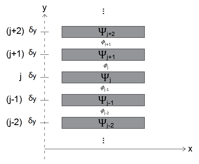
Figure 1: Sketch of a 1D-BEC array showing the order parameters $\Psi_{j}(x,t)=\sqrt{n_{j}(x,t)}\exp{[i\theta_{j}(x,t)]}$ along each component $j$, and the relative phases $\phi_{j}(x,t)=\theta_{j+1}-\theta_{j}$ along the junctions. The discrete $y$-direction is effectively built through the characteristic length $\delta y=\sqrt{\hbar/m\Omega}$ determined by the coherent coupling of frequency $\Omega$ between components.

We consider a system of $M$ 1D BECs having a coherent linear coupling of frequency $\Omega$ along the junctions. Each BEC is described by a corresponding order parameter $\Psi_{j}(x,t)=\sqrt{n_{j}(x,t)}\exp{[i\theta_{j}(x,t)]}$, where $n_{j}$ and $\theta_{j}$ are the local density and phase, respectively, and $j=1,2,...M$ labels the BECs in the stack. We choose a particular arrangement with periodic boundary conditions, so that the stack has a ring-shaped configuration with also $M$ coupling junctions. The $j$-th junction lies between the $j$-th and the $(j+1)$-th components, and the $M$-th junction connects the $M$-th and the $1$-st BECs. The total density of the system, $n_{T}(x)=\sum_{j}\left|\Psi_{j}\right|^{2}$, is normalized to the total number of particles, $N=\int n_{T}\,dx=\sum_{j}N_{j}$, which is a conserved quantity, and $N_{j}$ is the number of particles in the $j$-th BEC. A schematic representation of the system is shown in Fig. 1. Detailed proposals for the experimental realization of such systems in ultracold gases Baals et al. (2018), including a gauge dependent coupling Budich et al. (2017), have been recently presented.

At zero temperature, within the mean-field framework, the system can be described by a set of coupled Gross-Pitaevskii (GP) equations, namely for the $j$-th component:

$$i\hbar\frac{\partial\Psi_{j}}{\partial t}=\left(\frac{-\hbar^{2}}{2m}\partial_{x}^{2}+g\left|\Psi_{j}\right|^{2}\right)\Psi_{j}-\frac{\hbar\Omega}{2}\sum_{l=j-1}^{j+1}\Psi_{l}\,,$$ (1)

where the sum on the right hand side extends to the first neighbours $(j-1)$ and $(j+1)$, and $m$ is the bosonic mass. The 1D particle interaction strength is $g=2\hbar\omega_{\perp}a$, the $s$-wave scattering length is assumed to be repulsive $a>0$, and $\omega_{\perp}$ is the frequency of a tight transverse trap.

For a later discussion, it is convenient to rewrite the GP Eq. (1) in hydrodynamic form, in terms of the densities and phases:

$$\frac{\partial n_{j}}{\partial t} =-\frac{\partial}{\partial x}(n_{j}{v}_{j})$$

$$-\Omega\left(\sqrt{n_{j}\,n_{j+1}}\,\sin\phi_{j}-\sqrt{n_{j}\,n_{j-1}}\,\sin\phi_{j-1}\right)\,,$$ (2)

$$-\!\hbar\frac{\partial\theta_{j}}{\partial t} =\mathcal{Q}_{j}+\frac{m\,{v}_{j}^{2}}{2}+gn_{j}$$

$$-\frac{\hbar\Omega}{2}\left(\sqrt{\frac{n_{j+1}}{n_{j}}}\,\cos\phi_{j}+\sqrt{\frac{n_{j-1}}{n_{j}}}\,\cos\phi_{j-1}\right),$$ (3)

where $\phi_{j}=\theta_{j+1}-\theta_{j}$ is the relative phase between neighbor BECs, ${v}_{j}=\hbar\,{\partial_{x}}\theta_{j}/m$ is the superfluid velocity, and $\mathcal{Q}_{j}=-(\hbar^{2}/2m\sqrt{n_{j}})\partial_{x}^{2}\sqrt{n_{j}}$ is the quantum-pressure energy term.

Equation (2) is the continuity equation, and expresses the particle conservation in the array. The local density $n_{j}(x)$ varies due to either changes in the axial current, $J_{j}(x)=n_{j}(x)v_{j}(x)$, within the $j$-th BEC, or due to the Josephson current, $\mathcal{J}_{j}$, across the adjacent junctions. We define the latter current, by analogy with the axial current, as $\mathcal{J}_{j}(x)=\mathcal{N}_{j}(x)\,\mathcal{V}_{j}(x)$, by means of a geometric-mean density $\mathcal{N}_{j}=\sqrt{n_{j}\,n_{j+1}}$, and a Josephson velocity $\mathcal{V}_{j}=({\hbar}/{m\,\delta y})\sin\phi_{j}$, where $\delta y=\sqrt{\hbar/m\Omega}$ is the effective distance between BECs. With these definitions, the last term of Eq. (2) corresponds to a discrete derivative $\delta\mathcal{J}_{j}/\delta y=(\mathcal{J}_{j}-\mathcal{J}_{j-1})/\delta y$ of the Josephson current. Along with the periodic boundary conditions in the $y$-direction, it allows for the computation of a velocity circulation around the stack

$$\Gamma=\oint v_{y}\,dy=\delta y\sum_{j=1}^{M}\mathcal{V}_{j}=\frac{\hbar}{m}\sum_{j=1}^{M}\sin\,\phi_{j}\,.$$ (4)

On the other hand, Eq. (3) is the equation of motion for the phase, which varies locally according to the local energy content. In a stationary state, where the time variation of the phase is given by the frequency $\mu/\hbar$ (see Eq. (5) below), $\mu$ being the chemical potential, the local energy in the right hand side of Eq.(3) is the same (and equals $\mu$) at every point in the system.

III Stationary states

The BEC stack forms a discrete lattice of $M$ sites along the $y$-direction, transverse to the common axial $x$-axis (see Fig. 1). Since the effective (coupling-dependent) distance of separation between neighbor BECs is $\delta y$, the discrete coordinate along the $y$-axis takes values $y_{j}=j\delta y$ for each $j$-th BEC. The characteristic length $\delta y$ has to be compared with the healing length $\xi=\hbar/\sqrt{m\,g\,n}$, determined by the axial density $n$ of the BECs, so that the ratio $\xi/\delta y=\sqrt{\hbar\Omega/gn}$ measures the tunneling-coupling strength.

III.1 Bloch states

The lattice configuration along $y$ allows us to look for stationary states that take the form of transverse Bloch waves

$$\Psi_{j,k}(x,t)=\psi(x)\exp{[i(\mathcal{K}_{k}y_{j}-\mu_{\mathbf{k}}t/\hbar)]}\,,$$ (5)

where $\psi(x)$ is the axial wavefunction (with the periodicity of the discrete lattice), and $\mathcal{K}_{k}$ is the transverse quasimomentum. Due to the discreteness of the system, the quasimomentum can take only $M$ different integer values within the first Brillouin zone:

$$\mathcal{K}_{k}=\frac{2\pi}{M\delta y}\times k,\;\;\mbox{and}\;\;k\in\left\{0,\,\pm 1,\,\pm 2,\dots,\lfloor{M}/{2}\rfloor\right\}\,,$$ (6)

where $\lfloor{M}/{2}\rfloor$ is the greatest integer less than or equal to $M/2$. As a result, the product space of coordinate-separated solutions (5) presents an $M$-fold symmetry for each wave function $\psi(x)$. All the $k$ states but $k=0$ and $k=M/2$ (when the latter exists), at the middle and at the end, respectively, of the Brillouin zone, are states supporting Josephson currents in the $y$-direction, due to the existence of nonzero and non-$\pi$ relative phases between consecutive condensates.

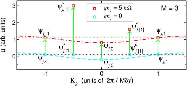
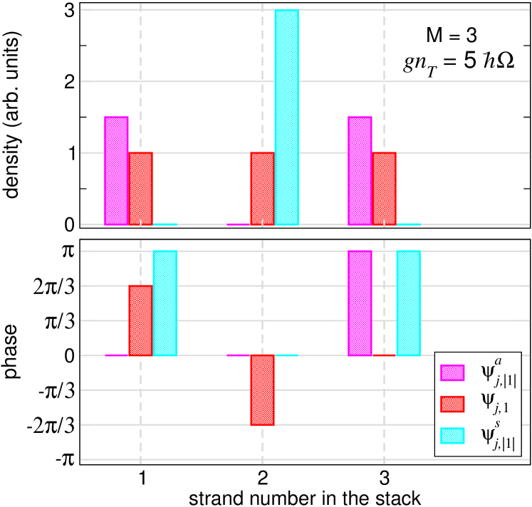
Figure 2: Stationary states in a stack made of $M=3$ coupled BECs with zero axial momentum, constant axial density, and total-interaction-to-coupling ratio $g\,n_{T}/{\hbar\Omega}=5$. Top panel: Chemical potential of Bloch waves $\Psi_{j,k}$, with definite transverse quasimomentum indices $k=0,\,\pm 1$ as given by the horizontal axis, and standing waves $\Psi_{j,|1|}^{a}$ and $\Psi_{j,|1|}^{s}$, without definite quasimomentum (the horizontal axis does not apply) and originated at $g\,n_{T}/{\hbar\Omega}=0$ from linear combinations of Bloch waves with $|k|=1$. The vertical arrows indicate the increment in chemical potential obtained by the respective states from an equal increment in the total interaction $gn_{T}=5\hbar\Omega$ over the non-interacting limit. Bottom panels: Density and phase of the Bloch waves with $k=1$ (red bars) and standing waves with $|k|=1$ (cyan and magenta bars) in each strand $j=1,\,2,\,3$. The (not represented) states $k=0,\,-1$ have, $\forall j$, $|\Psi_{j,0}|=|\Psi_{j,-1}|=|\Psi_{j,1}|$, $\arg(\Psi_{j,0})=0$, and $\arg(\Psi_{j,-1})=-\arg(\Psi_{j,1})$.

In what follows we focus on states whose axial part is a momentum eigenstate $\psi(x)=\sqrt{n}\exp(i\mathcal{K}_{x}\,x)$. The corresponding Bloch waves read

$$\Psi_{j,k}(x,t)=\sqrt{n}\,\exp{[i(\mathcal{K}_{x}\,x+\mathcal{K}_{k}y_{j}-\mu_{\mathbf{k}}t/\hbar)]}\,,$$ (7)

with stationary phases $\theta_{j}=\mathbf{k\cdot r}=\mathcal{K}_{x}\,x+\mathcal{K}_{k}y_{j}$, where $\mathbf{k}$ and $\mathbf{r}$ are the momentum and spatial vectors, respectively. The relative phases of the Bloch waves (7) are $\phi=\mathcal{K}_{k}\delta y=\pm 2\pi k\,/M$, the same for all the $j$ junctions, and take values in the interval $(-\pi,\pi]$. Thus, the Josephson currents are $\mathcal{J}=\pm\hbar\,n\sin(2\pi k\,/M)/m\delta y$, which in the limit of large $M$ and small $k$ tend to $\mathcal{J}=n\,\hbar\,\mathcal{K}_{k}/m$. Analogously, the transverse circulation Eq. (4) gives $\Gamma_{k}=\pm M\,\hbar\,\sin(2\pi k\,/M)/m$, and tends to $\Gamma_{k}=2\pi\,k\,\hbar/m$ in the same limit. The latter expression is equivalent to the quantized circulation of a regular vortex of charge $k$. We will refer to these discrete vortex currents, associated with Bloch waves having a non-zero circulation in the stack, as Josephson vortices. Note that they are delocalized along the $x$-direction, and, unlike the regular vortices, do not show in general an integer-valued circulation in units of $h/m$.

By substituting the constant density states of the type (7) in Eq. (1), or alternatively in Eq. (3), we get the chemical potential of such Bloch waves

$$\mu_{\mathbf{k}}=gn+\frac{\hbar^{2}\mathcal{K}_{x}^{2}}{2m}-\hbar\Omega\cos\left(\frac{2\pi k}{M}\right)\,,$$ (8)

which takes values in the range $\mu_{\mathbf{k}}\in gn+\hbar^{2}\mathcal{K}_{x}^{2}/2m+[-\hbar\Omega,\,\hbar\Omega]$, within a discrete band of energy width $2\hbar\Omega$. For given total density and axial momentum, the ground state of the system is the Bloch wave with zero quasimomentum $\Psi_{j,0}$, lying at the bottom of the band with $\mu_{k=0}=gn+\hbar^{2}\mathcal{K}_{x}^{2}/2m-\hbar\Omega$. In the limit $2\pi k/M\ll 1$, expanding Eq. (8) up to quadratic terms one finds $\mu_{\mathbf{k}}=gn-\hbar\Omega+\hbar^{2}(\mathcal{K}_{x}^{2}+\mathcal{K}_{k}^{2})/2m$, which is a quadratic dispersion (as in a fully 2D continuous system) around the ground state. The top panel of Fig. 2 depicts the structure of the discrete band of Bloch waves in the simplest case with $\mathcal{K}_{x}=0$ for both the non-interacting ($gn_{T}=0$) and the interacting ($gn_{T}\neq 0$) regime of a stack with $M=3$. In the latter, the total interaction term ($gn_{T}=5\hbar\Omega$) is the same for all the represented states, which is equivalent to fix the whole number of particles $N$ in the system for given interaction strength $g$ and (finite) axial length. The open symbols, on the top of dashed lines representing Eq. (8) for a continuous index $k$, indicate the chemical potential of the Bloch waves $\Psi_{j,k}$ with $k=0,\,\pm 1$. The horizontal dotted lines serve as references for better seeing the energy degeneracies. The two lower panels of Fig. 2 plot also the density and phase of the nonlinear Bloch wave with $k=1$ (red bars) for each strand $j=1,\,2,\,3$ (which varies along the horizontal axis).

III.2 Standing waves: localized states

Along with the Bloch waves, which realize transverse current states with definite quasimomentum, the BEC stack admits standing-wave solutions without definite quasimomentum. Their existence can be tracked up to the non-interacting regime ($g=0$), where the standing waves can be built from linear combination of energy-degenerate Bloch waves (7) with same quasimomentum modulus $|k|$ Muñoz Mateo et al. (2019). Due to the finite size of the stack, such combinations break the lattice symmetry and show differences in the particle density between neighbor BECs, which lies at the origin of the localized-density states in periodic systems known as gap solitons Muñoz Mateo et al. (2019). It is also worth noticing that, when integrated over the axial direction, the array of coupled 1D BECs can be described by a discrete nonlinear Schrödinger model along the transverse $y$-coordinate, where the existence and stability of localized states have been extensively studied Flach and Gorbach (2008).

Within the non-interacting regime, for each pair of energy-degenerate Bloch states with equal $|k|$ one can build also a pair of independent linear combinations with equal weight, which we will denote by $\Psi_{j,|k|}^{s}$ and $\Psi_{j,|k|}^{a}$, that have continuation into the nonlinear regime. In this way, families of nonlinear states are built sharing the same topology (node patterns) as the linear state from which they are generated. The simplest example is the $(M=3)$-stack for the families of states originated at $g=0$ from the (real) symmetric $\Psi_{j,|1|}^{s}=\Psi_{j,1}+\Psi_{j,-1}\propto\cos(2\pi j/3)$ and antisymmetric $\Psi_{j,|1|}^{a}=\Psi_{j,1}-\Psi_{j,-1}\propto\sin(2\pi j/3)$ superpositions of Bloch waves with $|k|=1$. Since the stack has discrete translational symmetry along the $y$-direction, the states $\Psi_{j^{\prime},|1|}^{s}$ and $\Psi_{j^{\prime},|1|}^{a}$ with shifted indices $j^{\prime}=j+i$ for given $i=0,\,1,...,M-1$ (and $j^{\prime}=(j+i)\pmod{M}$ if $(j+i)>M$) are degenerate stationary states with density peaks and associated phase patterns at different lattice sites. Figure 2 shows the chemical potential (top panel), and the density and the phase (at $gn_{T}=5\hbar\Omega$, bottom panels) of states belonging to these families in a system with zero axial momentum. Contrary to the original Bloch waves $\Psi_{j,\pm 1}$ (either linear or nonlinear), which have equal density across the stack, the antisymmetric states contain a nodal strand $\Psi_{2,|1|}^{a}=0$ and two density peaks $\Psi_{1,|1|}^{a}=-\Psi_{3,|1|}^{a}$, whereas the symmetric states present a single density peak $n_{2,|1|}^{s}>(n_{3,|1|}^{s}=n_{1,|1|}^{s})$. As can be seen in the bottom panel of Fig. 2 for the symmetric state, the density localization increases as the states go deeper into the nonlinear regime. For the same total density $n_{T}$ in the stack, that is for the same total number of particles at given axial length (as represented in the top panel of Fig. 2), in the interacting case the symmetric states present higher chemical potential than the antisymmetric ones, which in turn have higher chemical potential than the Bloch waves $\Psi_{j,\pm 1}$.

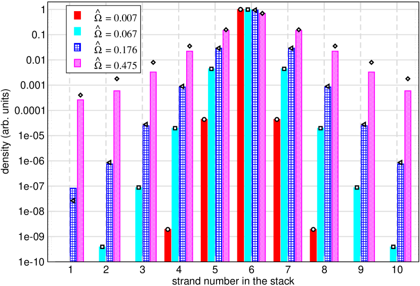
Figure 3: Stationary density profile of localized states with one density peak in a stack with $M=10$ and different ratios $\hat{\Omega}=\hbar\Omega/2gn$. The bars indicate the density of each BEC component as calculated from the numerical solution of the Gross-Pitaevskii equations (1), and the open symbols over the bars mark the corresponding value given by the approximation (10), derived in the small coupling regime $\hat{\Omega}\ll 1$. Density values below $10^{-10}$ are not shown.

Although other density-localized states can be built (for example, states presenting two adjacent density peaks in either in-phase or out-of-phase, staggered configuration, see e.g. Ref. Kivshar and Campbell (1993)), we will focus on states having either one density peak or two separated out-of-phase density peaks, for varying $M$, since they provide a representative sample for the study of the generic properties of localized states. As we will see in such states, for $M>3$ and in the small coupling limit $\hbar\Omega/2gn\ll 1$, where $n$ is now the maximum density in the stack, the mentioned density peaks accumulate practically the whole system density. In a symmetric state with $\mathcal{K}_{x}=0$, for instance, the nearest-neighbor BECs $j\pm 1$ of the peak-density strand $j$ follow stationary GP equations

$$g\,n_{j\pm 1}\,\psi_{j\pm 1}-\frac{\hbar\Omega}{2}(\psi_{j}+\psi_{j\pm 2})=\mu\,\psi_{j\pm 1}\,,$$ (9)

which, assuming decreasing amplitudes $\psi_{j}\gg\psi_{j\pm 1}\gg\psi_{j\pm 2}$, can be approximated up to first order in the neighbor amplitudes by $(\hbar\Omega/2)\psi_{j}\approx-\mu\,\psi_{j\pm 1}$, and $\mu\approx g\,n$. As a result, the $l$-site BECs have amplitudes decreasing in a factor

$$\frac{\psi_{l}}{\psi_{j}}=\left(-\frac{\hbar\Omega}{2gn}\right)^{|l-j|}\,,$$ (10)

for distances $|l-j|$ away from the density peak at $j$. The prototypical density profile is illustrated in Fig. 3, for different values of the coupling and same chemical potential, in a stack with $M=10$. The bars indicate the density at each $j$-th BEC as calculated from the numerical solution of the Gross-Pitaevskii equations, while the open symbols mark the values given by the analytical approximation Eq. (10). The same scenario takes place for the antisymmetric states with $M>4$, with decreasing amplitudes of opposite signs at both sides of the nodal strand.

IV Linear excitations

The almost lack of dissipation in ultracold-gas systems makes the dynamical stability of the stationary states the crucial issue for their experimental realization. For this reason, in this section we analytically address the linear stability of both Bloch waves and localized states in the stack, to be compared in next sections with their nonlinear dynamics. We make a general analysis based on the Bogoliubov equations for the linear excitations Pitaevskii and Stringari (2003) in order to find the stable regimes. For Bloch waves, we have also considered a long-wavelength excitation approach (whose derivation is deferred to the Appendix) to derive a resulting system of coupled sine-Gordon-like equations similar to usual models in superconducting Josephson junctions Mazo and Ustinov (2014).

IV.1 Linear stability of Bloch waves

Let us consider the linear excitations $[u_{j,k}(x),v_{j,k}(x)]$ with energy $\hbar\,\omega$ around the stationary states (7). After substituting $\Psi_{j,k}(x,t)=\exp{(-i\mu_{\mathbf{k}}t/\hbar)}[\sqrt{n}\exp{i\mathbf{(k\cdot r)}}+u_{j}(x)\exp{(-i\omega t)}+v^{*}_{j}(x)\exp{(i\omega t)}]$ in the GP equation (1), the excitation modes satisfy the Bogoliubov equations

$$H_{\mathbf{k}}\,u_{j}+\,g\,n\,e^{i2\mathbf{k\cdot r}}v_{j}-\frac{\hbar\Omega}{2}\left(u_{j-1}+u_{j+1}\right) =\hbar\omega\,u_{j}$$ (11)

$$-H_{\mathbf{k}}\,v_{j}-\,g\,n\,e^{-i2\mathbf{k\cdot r}}u_{j}+\frac{\hbar\Omega}{2}\left(v_{j-1}+v_{j+1}\right) =\hbar\omega\,v_{j}\,,$$ (12)

where $H_{\mathbf{k}}=-(\hbar^{2}/2m)\partial_{x}^{2}+2gn-\mu_{\mathbf{k}}$. By making use of the Fourier expansions $u_{j}(x)=\sum_{\mathbf{q}}c_{\mathbf{q}}\exp\{i[(\mathcal{K}_{x}+q_{x})x+(\mathcal{K}_{k}+q_{p})y_{j}]\}$ and $v_{j}(x)=\sum_{\mathbf{q}}d_{\mathbf{q}}\exp\{-i[(\mathcal{K}_{x}-q_{x})x+(\mathcal{K}_{k}-q_{p})y_{j}]\}$, where $q_{p}=2\pi p/M\delta y$ is the transverse momentum of the excitation for integer $p=0,\,\pm 1,\,\pm 2,\dots\lfloor M/2\rfloor$, the Bogoliubov equations get decoupled for each two-dimensional wave number $\mathbf{q}=(q_{x},q_{p})$:

$$\left[E_{\mathbf{k},+}-\hbar\Omega\cos\left(\frac{2\pi(k+p)}{M}\right)\right]c_{\mathbf{q}}+\,g\,n\,d_{\mathbf{q}} =\hbar\omega\,c_{\mathbf{q}}\,,$$ (13)

$$-\left[E_{\mathbf{k},-}-\hbar\Omega\cos\left(\frac{2\pi(k-p)}{M}\right)\right]d_{\mathbf{q}}-\,g\,n\,c_{\mathbf{q}} =\hbar\omega\,d_{\mathbf{q}}\,,$$ (14)

where $E_{\mathbf{k},\pm}=\hbar^{2}(q_{x}^{2}\pm 2\mathcal{K}_{x}\,q_{x})/2m+gn+\hbar\Omega\cos(2\pi\,k/M)$. Further, we introduce the linear combinations of modes $f_{\pm}^{(\mathbf{q})}=c_{\mathbf{q}}\pm d_{\mathbf{q}}$, so that

$$\left(\zeta_{q_{x}}+2gn+\hbar\Omega\,\alpha_{k,p}\right)f_{+}^{(\mathbf{q})}=\hbar\left(\omega-\mathcal{K}_{x}\frac{\hbar q_{x}}{m}-\Omega\,\beta_{k,p}\right)f_{-}^{(\mathbf{q})},$$ (15)

$$\left(\zeta_{q_{x}}+\hbar\Omega\,\alpha_{k,p}\right)f_{-}^{(\mathbf{q})}=\hbar\left(\omega-\mathcal{K}_{x}\frac{\hbar q_{x}}{m}-\Omega\,\beta_{k,p}\right)f_{+}^{(\mathbf{q})},$$ (16)

where $\zeta_{q_{x}}=\hbar^{2}q_{x}^{2}/2m$ is the kinetic energy of the modes along each 1D BEC, and the transverse excitations are defined through the parameters

$$\alpha_{k,p}=\cos\left(\frac{2\pi k}{M}\right)\left[1-\cos\left(\frac{2\pi p}{M}\right)\right],$$ (17)

and

$$\beta_{k,p}=\sin\left(\frac{2\pi k}{M}\right)\sin\left(\frac{2\pi p}{M}\right)\,.$$ (18)

Therefore, for each stationary state $\Psi_{k}$, by solving Eqs. (15) and (16) for the frequency $\omega$, we get the dispersion relation of linear excitations

$$\hbar\omega =\hbar\mathcal{K}_{x}\frac{\hbar q_{x}}{m}+\hbar\Omega\,\beta_{k,p}$$

$$\pm\sqrt{\left(\zeta_{q_{x}}+\hbar\Omega\,\alpha_{k,p}\right)\left(\zeta_{q_{x}}+\hbar\Omega\,\alpha_{k,p}+2gn\right)}\,,$$ (19)

composed of $M$ double branches corresponding to the different values of $p$, which indexes the quasimomentum excitation. Equation  (19) provides the general result, as a function of the parameters of the system $\{M,\,\Omega,\,gn\}$, for the linear stability of Bloch states with momentum $\mathbf{k}=(\mathcal{K}_{x},\mathcal{K}_{k})$ in a stack of coupled BECs. It gives rise to complex frequencies, associated to dynamical instabilities, for negative values of the expression inside the square root. These are modulational instabilities that break down the homogeneous density profile across the stack. They can only appear if $\alpha_{k,p}$ takes negative values, which occurs for $k>M/4$. Hence, all the Bloch states with constant density are dynamically stable if $k\leq M/4$, irrespective of the coupling $\Omega$. For increasing $M$, the first stable Josephson current ($k\neq 0$) states correspond to $M=4$ and $k=\pm 1$, which are discrete transverse vortices with circulation $\Gamma_{\pm 1}=\pm 4\hbar/m$ (see Sect. V below). This quasimomentum-dependence stability of the Bloch waves resembles similar features of the discrete nonlinear Schrödinger equation Kivshar and Campbell (1993); Kivshar and Peyrard (1992). As we show in Sects. V and VI by analyzing some particular examples, the stability features of Bloch states predicted by Eq. (19) are confirmed by the nonlinear dynamics as obtained from the numerical simulations of the time-dependent GP Eq. (1).

Among the dispersion branches of Eq. (19), the $p=0$ branch is always gapless (because $\alpha_{k,0}=\beta_{k,0}=0$), whereas the rest present energy gaps given (at $q_{x}=0$) by

$$\hbar\omega_{g}=\hbar\Omega\,\beta_{k,p}\pm\sqrt{\hbar\Omega\,\alpha_{k,p}\left(\hbar\Omega\,\alpha_{k,p}+2g\,n\right)}\,,$$ (20)

which show up even in the non-interacting ($g=0$) case. The speed of sound along each BEC (i.e. along the $x$ coordinate) can be calculated from the gapless branch of the dispersion in the long-wavelength limit. In the frame of reference moving with axial velocity $\hbar\mathcal{K}_{x}/m$, it is:

$$c=\left(\frac{\partial\omega}{\partial q_{x}}\right)_{q_{x}\rightarrow 0}=\sqrt{\frac{gn}{m}}\,.$$ (21)

These quantities, $\hbar\omega_{g}$ and $c$, are relevant for the energetic stability of the system, since they define thresholds, in energy and speed, respectively, for the superfluid excitation by external perturbations.

In order to solve for the excitation spectrum, we choose the usual Bogoliubov normalization, $\int dx\,(|u_{j}|^{2}-|v_{j}|^{2})=1$, for the modes $(u_{j},v_{j})$ that have real energy values. By selecting also real values for the Fourier amplitudes $c_{\mathbf{q}}$ and $d_{\mathbf{q}}$, it follows that $|c_{\mathbf{q}}|^{2}-|d_{\mathbf{q}}|^{2}=f_{+}^{(\mathbf{q})}\,f_{-}^{(\mathbf{q})}=1/L_{x}$, where $L_{x}$ is the axial length of the BECs. With this prescription we solve Eqs. (15)-(16) for the stable excitation modes

$$f_{+}^{(\mathbf{q})}=\pm\frac{1}{\sqrt{L_{x}}}\left(\frac{\zeta_{q_{x}}+\hbar\Omega\,\alpha_{k,p}}{\zeta_{q_{x}}+\hbar\Omega\,\alpha_{k,p}+2gn}\right)^{1/4}\,.$$ (22)

The unstable excitation modes are associated with the complex energies of Eq. (19). The corresponding normalization reads $\int dx\,(|u_{j}|^{2}-|v_{j}|^{2})=0$ Pitaevskii and Stringari (2003), and we set $\int dx\,|u_{j}|^{2}=1$. Then $d_{\mathbf{q}}=c_{\mathbf{q}}\,\exp(i2\varphi_{\mathbf{q}})$, and the unstable excitation modes are

$$f_{\pm}^{(\mathbf{q})}=\frac{1}{\sqrt{L_{x}}}[1\pm\exp(i2\varphi_{\mathbf{q}})]\,,$$ (23)

where, from Eqs. (15)-(16), the phase $\varphi_{\mathbf{q}}$ is given by

$$\varphi_{\mathbf{q}}=\mathrm{atan}\left(\pm\sqrt{-\frac{\zeta_{q_{x}}+\hbar\Omega\,\alpha_{k,p}+2gn}{\zeta_{q_{x}}+\hbar\Omega\,\alpha_{k,p}}}\,\right).$$ (24)

IV.1.1 Limit of long-wavelength excitations and small coupling.

As follows from the hydrodynamic approach for the linear excitations of Bloch waves developed in the Appendix, in the long-wavelength regime and small Josephson coupling, $(\hat{\Omega}=\hbar\Omega/2gn)\ll 1$, the equations of motion for excitations in the relative phase $\phi_{j}$ and relative density $\rho_{j}$ become:

$$\frac{1}{c^{2}}\frac{\partial^{2}\rho_{j}}{\partial t^{2}}-\frac{\partial^{2}\rho_{j}}{\partial x^{2}}-\alpha_{k}\frac{\delta^{2}\rho_{j}}{\delta y^{2}}=0\,,$$ (25)

$$\frac{1}{c^{2}}\frac{\partial^{2}\phi_{j}}{\partial t^{2}}-\frac{\partial^{2}\phi_{j}}{\partial x^{2}}-\alpha_{k}\frac{\delta^{2}\sin\phi_{j}}{\delta y^{2}}\!=\!\beta_{k}\frac{\rho_{j+1}-\rho_{j-1}}{\delta y^{2}}\,,$$ (26)

where $\alpha_{k}=\cos(2\pi\,k/M)$ and $\beta_{k}=\sin(2\pi\,k/M)$. This system of $M$ pairs of equations describes the linear dynamics of the underlying array of junctions determined by the GP Eqs. (1). The $k$-dependent factor $\alpha_{k}$ multiplying the transversal (discrete) derivative indicates a varying penetration length $\xi_{J,k}=\delta y/\sqrt{|\alpha_{k}|}$. The sine functions in Eq. (26) should be formally substituted by their arguments $\sin\phi_{j}\approx\phi_{j}$, since we have assumed a linear regime. By keeping them, we highlight the correspondence with a sine-Gordon-like equation, where kink solutions can be found Barone and Paterno (1982). As a limiting case, the kink-type solutions have demonstrated to be useful in the search of solitonic states in the nonlinear dynamics of two-component condensates Qadir et al. (2012); Brand and Shamailov (2018); Son and Stephanov (2002); Qu et al. (2017); Su et al. (2015).

Equations (25)-(26) admit plane wave solutions with the same phase shifts across the stack previously found in Eq. (6):

$$\rho_{j,k,p}(x,t) = c_{\mathbf{q}}\,\exp{[i(q_{x}x+q_{p}y_{j}-\omega_{k,p}\,t)]}\,,$$

$$\phi_{j,k,p}(x,t) = d_{\mathbf{q}}\,\exp{[i(q_{x}x+q_{p}y_{j}-\omega_{k,p}\,t)]}\,,$$ (27)

with transverse momentum $q_{p}=2\pi p/M\delta y$. After substitution, one gets the amplitude relation $c_{\mathbf{q}}=i\,\nu\,d_{\mathbf{q}}$, where $\nu$ is a real number, and the double-branched dispersion

$$\omega_{k,p}^{(1)}=c\,\sqrt{\,q_{x}^{2}+\frac{2}{\delta y^{2}}\,\alpha_{k,p}}\;\;,$$

$$\omega_{k,p}^{(2)}=c\,\sqrt{\,q_{x}^{2}+\frac{2}{\delta y^{2}}\,(\alpha_{k,p}+\nu\beta_{k,p})}\;\;.$$ (28)

For $\beta_{k}=0$ (that is, when $k=0$ or $k=M/2$, and $\alpha_{k}=\pm 1$) both branches coincide, in agreement with the Bogoliubov dispersion Eq. (19) in the small coupling limit, $\hat{\Omega}\ll 1$, considered here. The gaps are given by $\omega_{k,p}^{(1)}=c\sqrt{2\alpha_{k,p}}/\delta y$. Additionally, for $q_{p}\ll 1$ the dispersion can be written as $\omega_{k,p}=c\,\sqrt{q_{x}^{2}\pm q_{p}^{2}}$, which is the usual dispersion $\omega=c\,|\mathbf{q}|$ of a continuous (relativistic) 2D system when $k=0$, and contains instabilities when $k=M/2$ for $|q_{p}|>|q_{x}|$.

The second dispersion branch $\omega_{k,p}^{(2)}$, is not fully consistent with the Bogoliubov spectrum for $\beta_{k,p}\neq 0$, unless $\nu=1$ and the limit $\hbar\Omega\rightarrow 0$ were considered. Such inconsistencies have been previously found in two coupled condensates (see e.g. Abad and Recati (2013)), and arise from neglecting the quantum pressure term. As a consequence, and as usual within this approximation, the validity of this hydrodynamic model gets restricted to the lowest energy excitations (long-wavelength excitation modes of the lowest energy branch), which is equivalent to consider decoupled wave equations (25)and (26), neglecting the right hand side of the latter, for the relative densities and phases.

IV.2 Linear stability of localized states

We study the stability of the previously introduced standing-wave states having one or two density peaks in the stack of constant density BECs. The analysis of the simplest systems with $M=3,\,4$ components serves as an insightful starting point, with straightforward analytical solutions for the antisymmetric states. For a generic $M$ value, we focus on the small coupling limit $(\hat{\Omega}=\hbar\Omega/2gn)\ll 1$, where now $n$ is the peak (or maximum) density in the stack.

The wavefunctions of the antisymmetric states with $M=3$ are: $\Psi_{2,|1|}^{a}=0$ and $\Psi_{3,|1|}^{a}=-\Psi_{1,|1|}^{a}=\sqrt{n}\,\exp[i(\mathcal{K}_{x}\,x-\mu_{|1|}^{a}t/\hbar)]$, where the chemical potential is $\mu_{|1|}^{a}=\hbar^{2}\mathcal{K}_{x}^{2}/2m+gn+\hbar\Omega/2$. Note that the stationary phase pattern of these nonlinear states (for $\mathcal{K}_{x}=0$ and $t=0$) is determined by the corresponding linear state of this family (at $g=0$), in this case we set $\Psi_{j,|1|}^{a}\propto\sin(2\pi\,(j+1)/3)$. Two pairs of Bogoliubov equations are obtained, namely for the first BEC with $j=1$:

$$H_{|1|}^{a}\,u_{1}+\,g\,n\,e^{i2\mathcal{K}_{x}x}v_{1}-\frac{\hbar\Omega}{2}\left(u_{2}+u_{3}\right) =\hbar\omega\,u_{1}\,,$$ (29)

$$-H_{|1|}^{a}\,v_{1}-\,g\,n\,e^{-i2\mathcal{K}_{x}x}u_{1}+\frac{\hbar\Omega}{2}\left(v_{2}+v_{3}\right) =\hbar\omega\,v_{1}\,,$$ (30)

where $H_{|1|}^{a}=-(\hbar^{2}/2m)\partial_{x}^{2}+2gn-\mu_{|1|}^{a}$, and identical equations follow for the $j=3$ BEC component by swapping indexes $1$ and $3$; and for the nodal $j=2$ component

$$\left(-\frac{\hbar^{2}}{2m}\frac{\partial^{2}}{\partial x^{2}}-\mu_{|1|}^{a}\right)u_{2}-\frac{\hbar\Omega}{2}\left(u_{1}+u_{3}\right) =\hbar\omega\,u_{2}\,,$$ (31)

$$-\left(-\frac{\hbar^{2}}{2m}\frac{\partial^{2}}{\partial x^{2}}-\mu_{|1|}^{a}\right)v_{2}+\frac{\hbar\Omega}{2}\left(v_{1}+v_{3}\right) =\hbar\omega\,v_{2}\,.$$ (32)

As previously, making use of the Fourier expansions $u_{j}(x)=\sum_{q}c_{q}\exp\{i[(\mathcal{K}_{x}+q_{x})x]\}$ and $v_{j}(x)=\sum_{q}d_{q}\exp\{-i[(\mathcal{K}_{x}-q_{x})x]\}$, after some algebraic manipulations, we get the following six branches of the spectrum:

$$\hbar\omega_{|1|}^{a}=\;\hbar\mathcal{K}_{x}\frac{\hbar q_{x}}{m}\pm\sqrt{(\zeta_{q_{x}}-{\hbar\Omega})(\zeta_{q_{x}}-{\hbar\Omega}+2gn)},$$

$$\hbar\omega_{|1|}^{a}=\;\hbar\mathcal{K}_{x}\frac{\hbar q_{x}}{m}$$

$$\pm\sqrt{\left(\zeta_{q_{x}}-\frac{3\hbar\Omega}{2}\right)\left(\zeta_{q_{x}}-\frac{3\hbar\Omega}{2}\pm 2gn\gamma^{(3)}\right)-\lambda^{(3)}\frac{\hbar\Omega}{2}gn},$$ (33)

where $\gamma^{(3)}=\sqrt{(1-\hat{\Omega}/2)^{2}+2\hat{\Omega}^{2}}$, and $\lambda^{(3)}=1-9\hat{\Omega}/4$. As is apparent from the negative values of the radicand, the system is unstable.

The analysis is simpler for the antisymmetric states with $M=4$, where the wave functions are $\Psi_{3,|1|}^{a}=-\Psi_{1,|1|}^{a}=\sqrt{n}\,\exp[i(\mathcal{K}_{x}\,x-\mu_{|1|}^{a}t/\hbar)]$, and $\Psi_{2,|1|}^{a}=\Psi_{4,|1|}^{a}=0$, and the chemical potential does not depend on the coupling $\mu_{|1|}^{a}=\hbar^{2}\mathcal{K}_{x}^{2}/2m+gn$. Similar manipulations of the corresponding Bogoliubov equations as before, which coincide with Eqs. (29) to (32), lead to the eight branches of the spectrum

$$\hbar\omega_{|1|}^{a} =\;\hbar\mathcal{K}_{x}\frac{\hbar q_{x}}{m}\pm(\zeta_{q_{x}}-gn)\,,$$

$$\hbar\omega_{|1|}^{a} =\;\hbar\mathcal{K}_{x}\frac{\hbar q_{x}}{m}\pm\sqrt{\zeta_{q_{x}}(\zeta_{q_{x}}+2gn)}\,,$$ (34)

$$\hbar\omega_{|1|}^{a} =\;\hbar\mathcal{K}_{x}\frac{\hbar q_{x}}{m}\pm\left(\gamma^{(4)}\pm\sqrt{(\gamma^{(4)})^{2}-(\lambda^{(4)})^{2}}\right)^{\frac{1}{2}}\,,$$

where $\gamma^{(4)}=\zeta_{q_{x}}^{2}+(\hbar\Omega)^{2}+(gn/2)^{2}$ and $\lambda^{(4)}=[\zeta_{q_{x}}^{2}-(\hbar\Omega)^{2}-(gn)^{2}\,]^{2}-(gn)^{2}(\zeta_{q_{x}}-gn)^{2}$. Different to the $M=3$ case, and although the last expression in (34) can in general produce imaginary frequencies, it is still possible to find dynamically stable states (with only real frequencies) in the small coupling regime whenever $\lambda^{(4)}<\gamma^{(4)}$.

The symmetric states involve a more cumbersome algebra. For the simplest stack with $M=3$, the chemical potential is $\mu_{|1|}^{s}=\hbar^{2}\mathcal{K}_{x}^{2}/2m+(2gn_{1,|1|}^{s}+g\delta n_{1,|1|}^{s}-\hbar\Omega/2+\sqrt{(g\delta n_{1,|1|}^{s}+\hbar\Omega/2)^{2}+2(\hbar\Omega)^{2}\,})/2$, where $\delta n_{1,|1|}^{s}=n_{2,|1|}^{s}-n_{1,|1|}^{s}$ is the density contrast between components, which increases with the chemical potential for a given coupling. An asymptotic analysis can be readily done in the small coupling limit $\hat{\Omega}\ll 1$, where the densities fulfill $(n_{2,|1|}^{s}\approx n_{T})\gg(n_{1,|1|}^{s}=n_{3,|1|}^{s})$. Then $\Psi_{2,|1|}^{s}=\sqrt{n}\exp[i(\mathcal{K}_{x}\,x-\mu_{|1|}^{s}t/\hbar)]$ and $(\Psi_{1,|1|}^{s}=\Psi_{3,|1|}^{s})\approx-\hat{\Omega}\,\Psi_{2,|1|}^{s}$, and the chemical potential is $\mu_{|1|}^{s}\approx\hbar^{2}\mathcal{K}_{x}^{2}/2m+gn$. In this approximation, the Fourier expansion of the excitation modes leads to the same functional form of the spectrum (34) with the substitution of $\hbar\Omega$ by $\hbar\Omega/\sqrt{2}$. As a consequence, dynamical stability of the (one-peak) symmetric states is also expected in the small $\hat{\Omega}$ regime. In this case, the strong localization of the density in a single strand, with neighbor densities decreasing as powers of $\hat{\Omega}^{2}$, allows the stability prediction to be extended to arbitrary $M$, and even to systems with open boundary conditions. Furthermore, the same analysis also applies to the (two-peak) antisymmetric states with $M>4$. As we later demonstrate in Sect. VI, the numerical solutions of both the Bogoliubov equations for the linear excitations and the GP equation for the nonlinear time evolution confirm these predictions.

V Transverse Josephson vortices

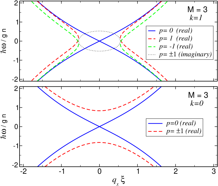
Figure 4: Dispersion relations for constant density states in a $M=3$ stack with $\hbar\Omega=0.2\,gn$ and $\mathcal{K}_{x}=0$. The $p$ index labels the excitation modes of each stationary state (see text). The horizontal axis measures the axial quasimomentum excitation $q_{x}$ in (inverse of) healing length $\xi$ units. Top panel: Energy excitations of the Bloch wave with $k=1$ and chemical potential $\mu_{1}/gn=1.1$. For the unstable modes $p=\pm 1$, only the imaginary part of the complex frequency $\hbar\,$Im($\omega$) is represented (dotted line). Bottom panel: Energy excitations of the ground state with $k=0$ and $\mu_{0}/gn=0.8$.

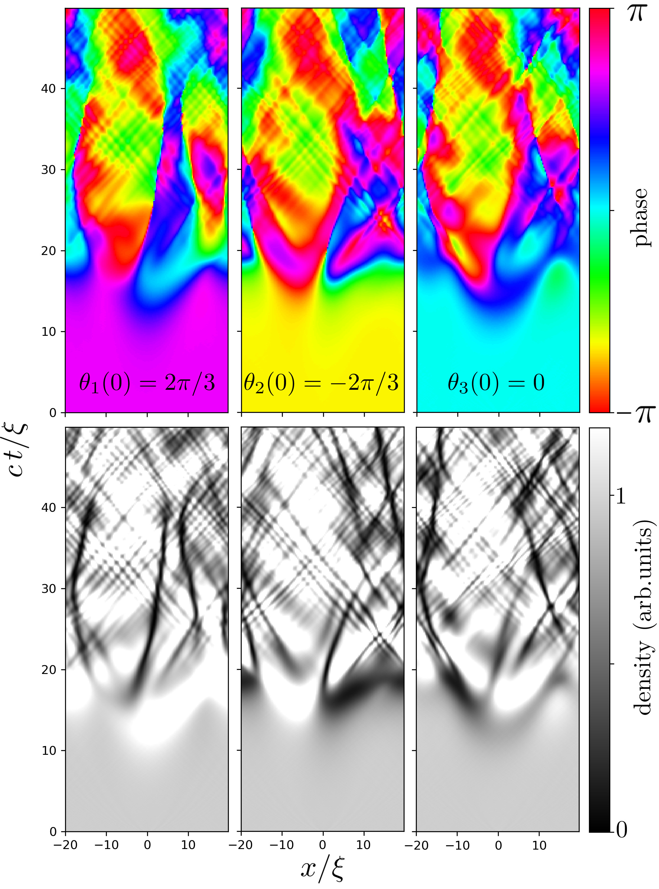
Figure 5: Decay of a Bloch state with $k=1$ and constant density in a $M=3$ stack with $\hbar\Omega=0.2\,gn$ and $\mathcal{K}_{x}=0$. The time evolution of the axial phases (top panels) and the axial densities (bottom panels) is shown for each BEC component, from left to right, $j=$1, 2, 3. The labels in the top panels indicate the corresponding phases $\theta_{j}$ of the stationary configuration. The initial state (at $t=0$) has been seeded with a random Gaussian perturbation (less than 1$\%$ in amplitude). On the horizontal axis, the axial length is measured in healing length $\xi$ units.

In this section we compare the stability predictions of the linear analysis for Bloch wave states with the numerical solutions of the GP Eq. (1) for representative sets of parameters. Just for the purpose of showing two different examples, we consider one case with zero axial momentum $\mathcal{K}_{x}=0$ and another with $\mathcal{K}_{x}\neq 0$. As we will see, the linear predictions coincide with the numerical results of the nonlinear dynamics, and in particular, stable transverse Josephson vortices (associated with Bloch waves having non-zero circulation) are found.

V.1 Case $M=3$ and $\mathcal{K}_{x}=0$

The Bloch waves have quasimomentum $\mathcal{K}_{k}$ for values of $k=0,\pm 1$. Let us analyze the solutions for each particular case:

• $k=0\,$: This is the ground state for given interaction strength and total density. All the components share the same wave function $\psi_{0}=\sqrt{n}\,\exp{(-i\mu_{0}t/\hbar)}$, with chemical potential $\mu_{0}=gn-\hbar\Omega$. By using the parameters $\alpha_{0,p}=\{0\,,3/2,\,3/2\}$ and $\beta_{0,p}=\{0,0,0\}$, with $p=0,\pm 1$, the dispersion curves, $\omega_{0,p}\,$, are

  $$\hbar\omega_{0,0} = \pm\sqrt{\zeta_{q_{x}}\left(\zeta_{q_{x}}+2gn\right)}\,,$$ (35)

  $$\hbar\omega_{0,\pm 1} = \sqrt{\left(\zeta_{q_{x}}+\frac{3\hbar\Omega}{2}\right)\left(\zeta_{q_{x}}+\frac{3\hbar\Omega}{2}+2gn\right)}\,.$$ (36)

  These expressions are plotted in the bottom panel of Fig. 4 for a system with $\hbar\Omega=0.2\,gn$. As expected, all the excitation energies are real, and the state is stable.

• $k=1\,$: The wave functions for the BEC components are:

  $$\psi_{1,1} =\sqrt{n}\,\exp{[i(2\pi/3-\mu_{1}t/\hbar)]}\,,$$ (37)

  $$\psi_{2,1} =\sqrt{n}\,\exp{[i(4\pi/3-\mu_{1}t/\hbar)]}\,,$$ (38)

  $$\psi_{3,1} =\sqrt{n}\,\exp{[i(2\pi-\mu_{1}t/\hbar)]}\,,$$ (39)

  which configure a discrete anti-vortex of circulation $\Gamma_{1}=-3\sqrt{3}\hbar/2m$ around the discrete $y$-direction. Analogously, the Bloch wave with $k=-1$ corresponds to an (energetically degenerate) vortex with opposite circulation $\Gamma_{-1}=-\Gamma_{1}$. The chemical potential is $\mu_{1}=gn+\hbar\Omega/2$ and the parameters $\alpha_{1,p}=\{0\,,-3/4,\,-3/4\}$ and $\beta_{1,p}=\{0\,,3/4,\,-3/4\}$. The resulting dispersion curves, $\omega_{1,p}\,$, are:

  $$\hbar\omega_{1,0} =\pm\sqrt{\zeta_{q_{x}}\left(\zeta_{q_{x}}+2gn\right)}\,,$$ (40)

  $$\hbar\omega_{1,1} =\frac{3\hbar\Omega}{4}$$ (41)

  $$\pm\sqrt{\left(\zeta_{q_{x}}-\frac{3\hbar\Omega}{4}\right)\left(\zeta_{q_{x}}-\frac{3\hbar\Omega}{4}+2gn\right)}\,,$$

  $$\hbar\omega_{1,-1} =-\frac{3\hbar\Omega}{4}$$ (42)

  $$\pm\sqrt{\left(\zeta_{q_{x}}-\frac{3\hbar\Omega}{4}\right)\left(\zeta_{q_{x}}-\frac{3\hbar\Omega}{4}+2gn\right)}\,.$$

  The upper panel of Fig. 4 depicts these expressions for a system with $\hbar\Omega=0.2\,gn$. For $\omega_{1,\pm 1}\,$, the negative signs under the square root indicate the presence of instabilities on the vortex state. An example of the decay dynamics of this unstable vortex state is shown in Fig. 5. The graph depicts the real time evolution of the system after imprinting a small random perturbation on the stationary state. The data, axial phases (top panels) and axial densities (bottom panels) for each component, have been obtained from the numerical solution of the GP Eqs. (1) with periodic boundary conditions in the axial coordinate, given in units of the healing length $\xi$. As can be seen, the stationary configuration survives for a time lapse of around $t\approx 10\,\xi/c$, beyond which soliton-like structures (tracing thick, dark paths on the axial density plots) appear, producing strong density and phase modulations. Different noise seeds on the initial state produce different density and phase patterns during the decay dynamics, with the only common feature of the emergence of several, interacting solitons.

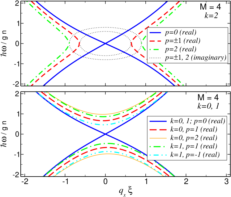
Figure 6: Same as Fig. 4 for constant density states in a $M=4$ stack with $\hbar\Omega=0.2\,gn$ and $\mathcal{K}_{x}\,\xi=0.1$. The top panel corresponds to the (unstable) Bloch wave with $k=2$, whereas the bottom panel shows the linear excitations of the (stable) Bloch waves with $k=0$ and $k=1$. Only the imaginary part (dotted curves) is plotted for the unstable frequencies.

V.2 Case $M=4$ and $\mathcal{K}_{x}\neq 0$: stable Josephson vortices with $k=\pm 1$

Here we consider arbitrary axial momentum ($\mathcal{K}_{x}$) states. The Bloch waves have $k=0,\pm 1,\,2$, and the excitation modes have also $p=0,\pm 1,2$.

• $k=0\,$: This corresponds to the ground state for a given $\mathcal{K}_{x}$, $\psi_{0}=\sqrt{n}\,\exp{(i\mathcal{K}_{x}\,x-i\mu_{0}t/\hbar)}$, with chemical potential $\mu_{0}=gn+{\hbar^{2}\mathcal{K}_{x}^{2}}/{2m}-\hbar\Omega$, and system parameters $\alpha_{0,p}=\{0\,,1,\,1,\,2\}$ and $\beta_{0,p}=\{0,0,0,0\}$. The dispersion curves read:

  $$\hbar\omega_{0,0} =\frac{\hbar^{2}\mathcal{K}_{x}q_{x}}{m}\pm\sqrt{\zeta_{q_{x}}\left(\zeta_{q_{x}}+2gn\right)}\,,$$ (43)

  $$\hbar\omega_{0,\pm 1} =\frac{\hbar^{2}\mathcal{K}_{x}q_{x}}{m}$$ (44)

  $$\pm\sqrt{\left(\zeta_{q_{x}}+{\hbar\Omega}\right)\left(\zeta_{q_{x}}+{\hbar\Omega}+2gn\right)}\,,$$

  $$\hbar\omega_{0,2} =\frac{\hbar^{2}\mathcal{K}_{x}q_{x}}{m}$$

  $$\pm\sqrt{\left(\zeta_{q_{x}}+2{\hbar\Omega}\right)\left(\zeta_{q_{x}}+2{\hbar\Omega}+2gn\right)}\,.$$ (45)

  These expressions are plotted in the bottom panel of Fig. 6 for a system with $\hbar\Omega=0.2\,gn$ and $\mathcal{K}_{x}\,\xi=0.1$.

• $k=1\,$: The chemical potential is $\mu_{1}=gn+{\hbar^{2}\mathcal{K}_{x}^{2}}/{2m}$, and $\alpha_{1,p}=\{0,0,0,0\}$, $\beta_{1,p}=\{0\,,1,\,-1,\,0\}$. The wave functions are:

  $$\psi_{1,1} =\,-\psi_{3,1}=i\sqrt{n}\,\exp{[i(\mathcal{K}_{x}\,x-\mu_{1}t/\hbar)]}\,,$$

  $$\psi_{4,1} =\,-\psi_{2,1}=\sqrt{n}\,\exp{[i(\mathcal{K}_{x}\,x-\mu_{1}t/\hbar)]}\,,$$ (46)

  which yield a discrete, transverse vortex of circulation $\Gamma_{1}=4\hbar/m$. The interesting property of this state is its stability, irrespective of the axial momentum, which allows for its experimental realization. The dispersion curves $\omega_{1,p}$ contain only real frequencies (see Fig. 6):

  $$\hbar\omega_{1,0}=\hbar\omega_{1,2}=\frac{\hbar^{2}\mathcal{K}_{x}q_{x}}{m}\pm\sqrt{\zeta_{q_{x}}\left(\zeta_{q_{x}}+2gn\right)}\,,$$ (47)

  $$\hbar\omega_{1,1}=\hbar\left(\frac{\hbar\mathcal{K}_{x}q_{x}}{m}+\Omega\right)\pm\sqrt{\zeta_{q_{x}}\left(\zeta_{q_{x}}+2gn\right)}\,,$$ (48)

  $$\hbar\omega_{1,-1}=\hbar\left(\frac{\hbar\mathcal{K}_{x}q_{x}}{m}-\Omega\right)\pm\sqrt{\zeta_{q_{x}}\left(\zeta_{q_{x}}+2gn\right)}\,.$$ (49)

  We have also performed numerical simulations of the real time evolution of these states for $\hbar\Omega=0.2\,gn$ and $\mathcal{K}_{x}\,\xi=0.1$ (same parameters as in Fig. 6). Our numerical results obtained from the solution of the GP Eqs. (1), after seeding a random perturbation in the stationary state, confirm the dynamical stability of this state, since the initial configuration (46) keeps robust against the perturbations.

• $k=2\,$: This state lies at the edge of the Brillouin zone, having maximum chemical potential $\mu_{2}=gn+{\hbar^{2}\mathcal{K}_{x}^{2}}/{2m}+\hbar\Omega$, and parameters $\alpha_{2,p}=\{0\,,-1,\,-1,\,-2\}$ and $\beta_{2,p}=\{0,0,0,0\}$. The wave function in each BEC component is:

  $$\psi_{1,2} = \psi_{3,2}=\sqrt{n}\,\exp{[i(\mathcal{K}_{x}\,x-\mu_{2}t/\hbar)]}\,,$$ (50)

  $$\psi_{2,2} = \psi_{4,2}=-\sqrt{n}\,\exp{[i(\mathcal{K}_{x}\,x-\mu_{2}t/\hbar)]}\,.$$ (51)

  In this state the Josephson circulation vanishes, $\Gamma_{2}=0$, and the system presents a sequence of $\pi-$Josephson junctions which are unstable. This feature is captured by the linear dispersion, which shows several unstable branches

  $$\hbar\omega_{2,0} =\frac{\hbar^{2}\mathcal{K}_{x}q_{x}}{m}\pm\sqrt{\zeta_{q_{x}}\left(\zeta_{q_{x}}+2gn\right)}\,,$$ (52)

  $$\hbar\omega_{2,\pm 1} =\frac{\hbar^{2}\mathcal{K}_{x}q_{x}}{m}$$ (53)

  $$\pm\sqrt{\left(\zeta_{q_{x}}-\hbar\Omega\right)\left(\zeta_{q_{x}}-\hbar\Omega+2gn\right)}\,,$$

  $$\hbar\omega_{2,2} =\frac{\hbar^{2}\mathcal{K}_{x}q_{x}}{m}$$

  $$\pm\sqrt{\left(\zeta_{q_{x}}-2\hbar\Omega\right)\left(\zeta_{q_{x}}-2\hbar\Omega+2gn\right)}\,.$$ (54)

  Again our numerical simulations with the time-dependent GP Eqs. (1), for such a state with $\hbar\Omega=0.2\,gn$ and $\mathcal{K}_{x}\,\xi=0.1$, confirm the linear prediction and show the decay of the initial, constant density state.

VI Nonlinear dynamics of localized states

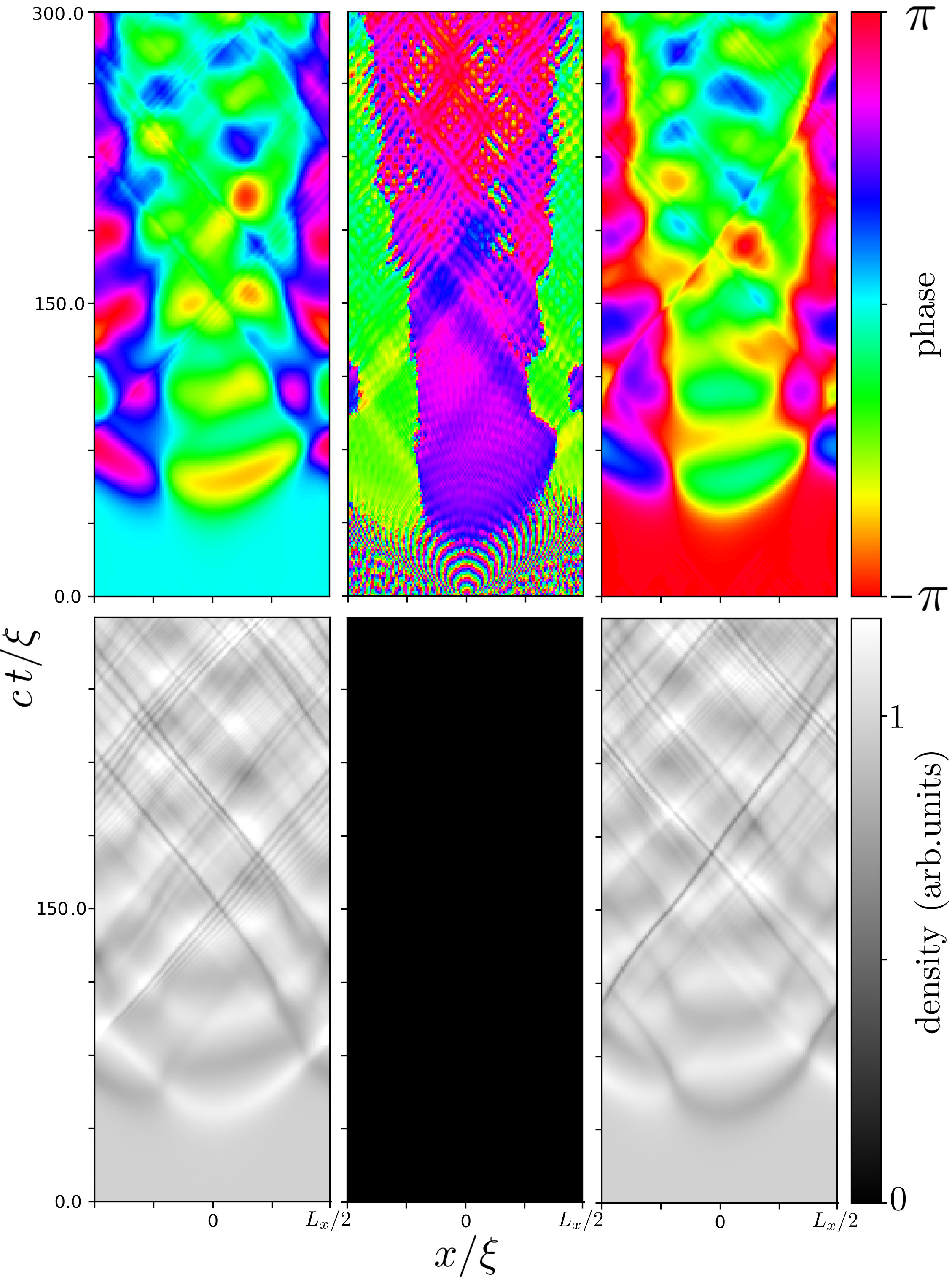
Figure 7: Time evolution of an antisymmetric state of the family $|k|=1$ and zero axial momentum in a $M=3$ stack of axial length $L_{x}=155\,\xi$ with periodic boundary conditions. Despite the small coupling, $\hbar\Omega=4\times 10^{-3}\,gn$, the system is dynamically unstable. The BECs $j=$1, 2, 3 correspond to the panels from left to right. The initial state has been seeded with a random Gaussian perturbation (less than 1$\%$ in amplitude).

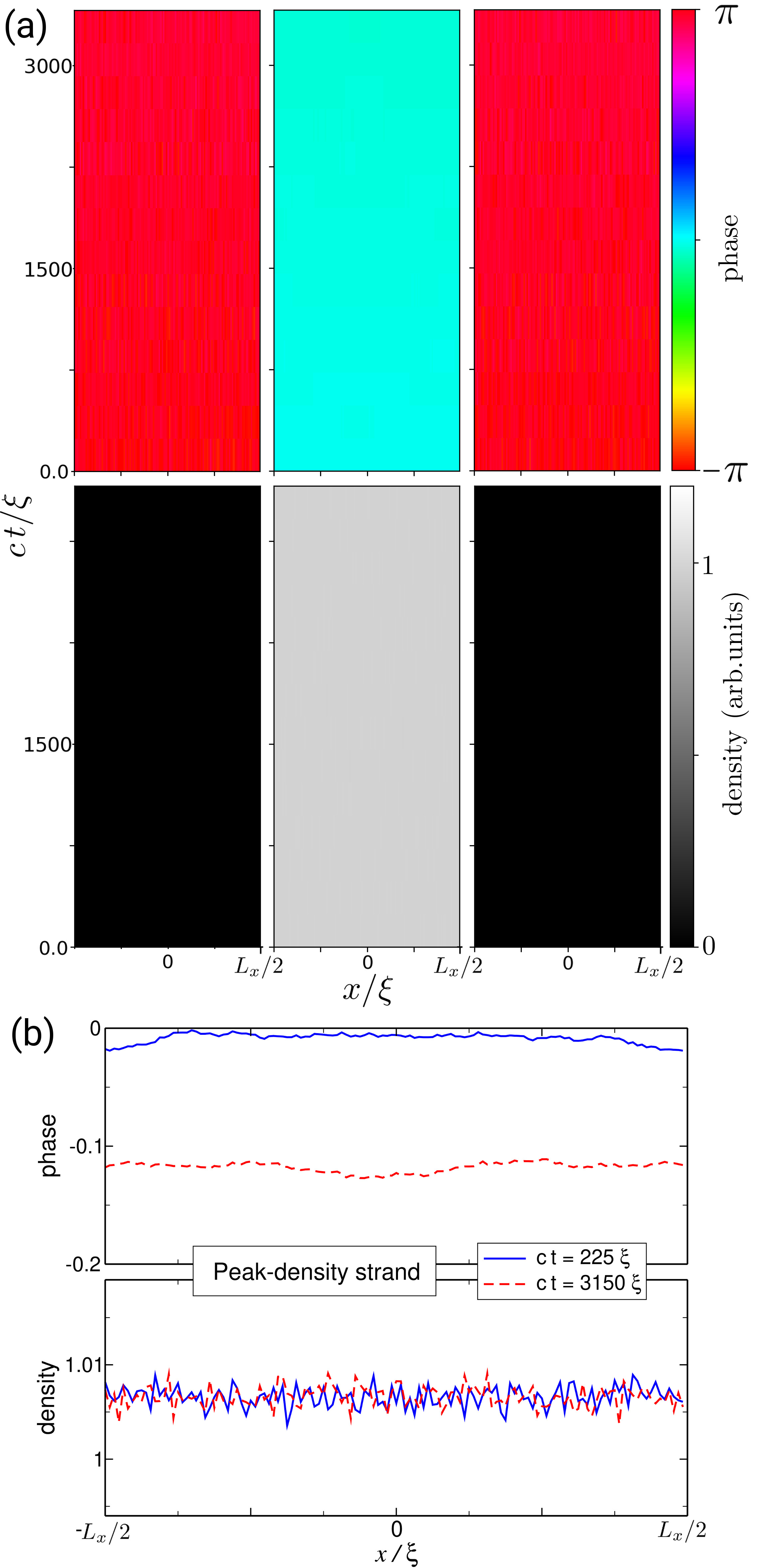
Figure 8: Time evolution of a stable, one-peak-symmetric state with zero axial momentum in a $M=10$ stack with the same parameters as the case of Fig. 7. (a) The phase (top) and density (bottom) of the peak-density strand (middle) and the two adjacent strands (sides) are shown. (b)Two snapshots at different times of the local density (bottom panel) and the local phase (top panel) of the peak-density strand during the time evolution with initial perturbative noise.

We study the nonlinear dynamics of the localized states with one or two density peaks in the stack of constant density BECs. First, we numerically solve the Bogoliubov equations in order to check the linear stability of the corresponding stationary state. Next, we perform the real time evolution with the GP Eq. (1) of this state after adding perturbative noise.

As predicted by the linear analysis of Sect. IV.2, in the simplest stack with $M=3$, the nonlinear dynamics of the antisymmetric states is unstable. To illustrate a typical decay process, Fig. 7 shows the real time evolution of an antisymmetric state with small coupling, $\hbar\Omega=4\times 10^{-3}\,gn$, and zero axial momentum, $\mathcal{K}_{x}=0$. The data have been obtained from the numerical solution of GP Eq. (1) with periodic boundary conditions in the axial coordinate. The axial length is $L_{x}=155\,\xi$. As can be seen, the initial nodal strand (middle panels in Fig. 7) remains unpopulated during the whole evolution, and its phase is essentially undefined. The decay process is qualitatively different to the Bloch wave case presented in Fig. 5. The asymmetric state shows robust features of structural stability, roughly keeping the initial density pattern across the stack.

On the contrary, we have checked that the nonlinear evolution of the symmetric state with $M=3$, for the same parameters used above, is stable against perturbations. For larger stacks (we have performed simulations up to $M=11$), our numerical results show that both the antisymmetric states (with two density peaks) in stacks with $M\geq 4$, and the symmetric states (with one density peak) in stacks with $M\geq 3$ are also stable for the mentioned small coupling. However, the stability is lost at higher coupling values (at $\hbar\Omega\gtrsim 1\times 10^{-2}\,gn$ for the parameters mentioned before). As a case example of stability, the time evolution of a symmetric state in a stack with $M=10$ components is shown in Fig. 8. In the top panels (a), only the peak-density strand and its nearest neighbours are shown, since the other components have a practically null density. The initial, $t=0$, state has been seeded with perturbative noise, the detailed evolution of which at intermediate times is depicted on the bottom panels (b) for the peak-density strand. As can be seen, the initial localized configuration is robust against the perturbations. Due to the strong density localization, the dynamics is insensitive to the change in the boundary conditions. Our results show that a one-peak state with open-boundary conditions follows a dynamics which is indistinguishable from that shown in Fig. 8.

VII Discussion and conclusions

The rich phenomenology presented by the stacks of parallel Josephson junctions can be readily realized in ultracold atomic gases by means of 1D or 2D optical lattices Budich et al. (2017); Baals et al. (2018). These systems support nonlinear states whose dynamics reflects the interplay of continuous (along the axial $x$-direction of the BECs) and discrete (across the stack) features, and are promising candidates for pursuing technical applications with close similarities to superconducting and photonic devices. In this work, we have contributed to this goal and have demonstrated the existence and stability of simultaneous superfluid currents flowing through both directions of a 2D stack. While the translation invariance along the $x$-axis allows for the excitation of axial-momentum eigenstates, the periodic arrangement of Josephson junctions induced by the linear coupling permits transverse Bloch waves carrying tunneling supercurrents. If the stack shapes a closed loop, these Josephson currents around it yield non-regular vortices whose circulation is a generic non-integer multiple of $h/m$.

The dispersion relations of the transverse Josephson vortices have been obtained from the analytical solution of the linear Bogoliubov equations for the condensate excitations, and compared against the nonlinear time evolution of these states as given by the numerical solution of the Gross-Pitaeskii equation. In all the cases, the subsequent nonlinear dynamics is consistent with the stability predictions of the linear anaysis.

For the sake of comparison with the usual coupled-sine-Gordon-equation model for coupled superconductors, a further linear analysis of the transverse Josephson vortices has been performed in the hydrodynamic limit. As a result, we have derived linear wave-like equations for the relative phases and densities of the BEC components that resemble the mentioned model in the limit of small coupling.

We have also shown that the Josephson supercurrents are suppressed in steady states that break the symmetry of the discrete lattice and can present a strong localization across the stack. These nonlinear states belong to continues families of solutions to the Gross-Pitaevskii equation that can be tracked up to the non-interacting regime, where they are linear superposition of degenerate Bloch waves with opposite quasimomentum. Among these families, the gap-soliton-like states showing one or two dominant density peaks find dynamical stability in finite systems within a small coupling regime.

The exploration of different topologies in the stack, or the effect of exposing the system to synthetic gauge fields Budich et al. (2017), stand out as interesting ways of extending the present work that will be reported elsewhere.

*

Appendix: Long-wavelength excitations. Hydrodynamic approach

We start by introducing low energy perturbations [$\delta n_{j}(x,t),\delta\theta_{j}(x,t)$] around the density and the phase of an equilibrium state $\Psi_{j}=\sqrt{n_{j}}\exp(i\theta_{j})\longrightarrow\sqrt{n_{j}+\delta n_{j}}\exp(i\theta_{j}+i\delta\theta_{j})$. Then, we substitute the perturbed states in Eqs. (2) and (3), and keep terms up to first order in the perturbations. We focus on the analysis of Bloch states with $n_{j}=n$. The mentioned procedure leads to

$$\frac{1}{n}\frac{\partial\delta n_{j}}{\partial t}=-\frac{\hbar}{m}\frac{\partial^{2}\delta\theta_{j}}{\partial x^{2}}$$

$$-\Omega\left(\alpha_{k}(\sin\delta\theta_{j+1,j}-\sin\delta\theta_{j,j-1})+\beta_{k}\frac{\delta\bar{n}_{j+1,j}-\delta\bar{n}_{j,j-1}}{2n}\right),$$ (55)

$$\frac{\partial\delta\theta_{j}}{\partial t}=-\frac{g\delta n_{j}}{\hbar}$$ (56)

$$-\frac{\Omega}{2}\left(\beta_{k}(\sin\delta\theta_{j+1,j}+\sin\delta\theta_{j,j-1})-\alpha_{k}\frac{\delta n_{j+1,j}-\delta n_{j,j-1}}{2n}\right)\,,$$

where $\delta\theta_{lj}=\delta\theta_{l}-\delta\theta_{j}$, $\delta n_{lj}=\delta n_{l}-\delta n_{j}$, $\delta\bar{n}_{lj}=\delta n_{l}+\delta n_{j}$ are the perturbations in relative phase, relative density and total density, respectively, and $\alpha_{k}=\cos(2\pi\,k/M)$, $\beta_{k}=\sin(2\pi\,k/M)$. As usual in a long-wavelength approximation, we have dropped the quantum-pressure term in Eq. (56). For reasons that will become apparent later, we have kept the sine functions ($\sin\delta\theta_{lj}$) even in the linear approximation in order to track the Josephson currents, but they will be replaced by their argument (for consistency within the assumed first order approximation) at intermediate steps of the analytical derivations.

In what follows, we use the short notation $\rho_{j}=\delta n_{j+1,j}/n$, $\bar{\rho}_{j}=\delta\bar{n}_{j+1,j}/n$, $\phi_{j}=\delta\theta_{j+1,j}$, and also $\bar{\phi}_{j}=\delta\theta_{j+1}+\delta\theta_{j}$ for the total phase. Since these quantities appear explicitly in previous expressions, we look for their equations of motion by adding and subtracting Eqs. (55) and Eq. (56) for consecutive components. For the relative quantities we get

$$\frac{\partial\rho_{j}}{\partial t} =-\frac{\hbar}{m}\!\!\left[\!\frac{\partial^{2}\phi_{j}}{\partial x^{2}}+\!\alpha_{k}\frac{\delta^{2}\sin\phi_{j}}{\delta y^{2}}+\!\beta_{k}\frac{\rho_{j+1}-\rho_{j-1}}{2\,\delta y^{2}}\right]$$ (57)

$$\frac{\partial\phi_{j}}{\partial t} =-\frac{m\,c^{2}}{\hbar}\rho_{j}+$$

$$\frac{\hbar}{m}\left[\frac{\alpha_{k}}{4}\frac{\delta^{2}\rho_{j}}{\delta y^{2}}-\beta_{k}\frac{\sin\phi_{j+1}-\sin\phi_{j-1}}{2\,\delta y^{2}}\right]\,,$$ (58)

where the discrete operator $\delta^{2}$ acts as $\delta^{2}f_{j}=f_{j+1}-2f_{j}+f_{j-1}$. Exactly the same equations are obtained for the total quantities substituting $\rho$ by $\bar{\rho}$ and $\phi$ by $\bar{\phi}$.

As can be seen, relative and total quantities are decoupled in pairs of equations (57)-(58). Within each pair, by taking the time derivative of one of the equations and making use of the others, wave-like equations are obtained:

$$\frac{1}{c^{2}}\frac{\partial^{2}\rho_{j}}{\partial t^{2}}-\left((1+\hat{\Omega}\alpha_{k})\frac{\partial^{2}}{\partial x^{2}}+(\alpha_{k}+\hat{\Omega})\frac{\delta^{2}}{\delta y^{2}}\right)\rho_{j}$$

$$+\frac{\hat{\Omega}}{2}\left(\alpha_{k}\frac{\partial^{2}}{\partial x^{2}}+(\alpha_{k}^{2}-\beta_{k}^{2})\frac{\delta^{2}}{\delta y^{2}}\right)(\rho_{j+1}+\rho_{j-1})$$

$$-2\hat{\Omega}\beta_{k}\left(\frac{\partial^{2}}{\partial x^{2}}+\alpha_{k}\frac{\delta^{2}}{\delta y^{2}}\right)(\phi_{j+1}-\phi_{j-1})=0\,,$$ (59)

$$\frac{1}{c^{2}}\frac{\partial^{2}\phi_{j}}{\partial t^{2}}-\left((1+\hat{\Omega}\alpha_{k})\frac{\partial^{2}}{\partial x^{2}}+(\alpha_{k}+\hat{\Omega})\frac{\delta^{2}}{\delta y^{2}}\right)\phi_{j}$$

$$+\frac{\hat{\Omega}}{2}\left(\alpha_{k}\frac{\partial^{2}}{\partial x^{2}}+(\alpha_{k}^{2}-\beta_{k}^{2})\frac{\delta^{2}}{\delta y^{2}}\right)(\phi_{j+1}+\phi_{j-1})$$

$$-\beta_{k}\left(1-\frac{\hat{\Omega}}{2}\alpha_{k}\,\delta^{2}\right)\frac{\rho_{j+1}-\rho_{j-1}}{\delta y^{2}}=0\,,$$ (60)

where $\hat{\Omega}=\hbar\Omega/2gn$. This system of M pairs of equations describes the linear dynamics of the BEC stack in the limit of long-wavelength excitations.