Linear Stability of Inviscid Vortex Rings to Axisymmetric Perturbations

Abstract

We consider the linear stability to axisymmetric perturbations of the family of inviscid vortex rings discovered by Norbury (1973). Since these vortex rings are obtained as solutions to a free-boundary problem, their stability analysis is performed using recently-developed methods of shape differentiation applied to the contour-dynamics formulation of the problem in the 3D axisymmetric geometry. This approach allows us to systematically account for the effects of boundary deformations on the linearized evolution of the vortex ring. We investigate the instantaneous amplification of perturbations assumed to have the same the circulation as the vortex rings in their equilibrium configuration. These stability properties are then determined by the spectrum of a singular integro-differential operator defined on the vortex boundary in the meridional plane. The resulting generalized eigenvalue problem is solved numerically with a spectrally-accurate discretization. Our results reveal that while thin vortex rings remain neutrally stable to axisymmetric perturbations, they become linearly unstable to such perturbations when they are sufficiently “fat”. Analysis of the structure of the eigenmodes demonstrates that they approach the corresponding eigenmodes of Rankine’s vortex and Hill’s vortex in the thin-vortex and fat-vortex limit, respectively. This study is a stepping stone on the way towards a complete stability analysis of inviscid vortex rings with respect to general perturbations.

1 Introduction

Vortex rings are among the most ubiquitous vortex structures encountered in fluid mechanics, both in laminar and turbulent flows. They occur in flow phenomena arising in diverse situations such as aquatic propulsion (Dabiri, 2009), blood flow in the human heart (Kheradvar & Pedrizzetti, 2012; Arvidsson et al., 2016) and in detonations (Giannuzzi et al., 2016), to mention just a few. A typical situation leading to the formation of “thin” vortex rings is when a jet issues from an orifice (Maxworthy, 1977), which is also the design principle of the “vortex gun” (Graber, 2015). On the other hand, “fat” vortex rings have been invoked as models of steady wakes behind spherical objects (Gumowski et al., 2008). Under certain simplifying assumptions vortex rings are known to represent relative equilibria of the equations governing the fluid motion and the persistence of these states is determined by their stability properties. The goal of this investigation is to address this question in the context of an idealized inviscid model of a vortex ring.

Given their significance in nature and technology, vortex rings have received a lot of attention in the fluids-mechanics literature, both from the experimental and theoretical point of view (Akhmetov, 2009). However, since in the general setting of three-dimensional (3D) unsteady flows the Navier-Stokes system is analytically intractable, most investigations in such settings have been based on numerical studies. Analytical approaches are applicable subject to some simplifying assumptions, usually involving axisymmetry and steady state. Starting from the original work of Tung & Ting (1967), the effects of viscosity were considered by Saffman (1970); Berezovskii & Kaplanskii (1992); Fukumoto & Moffatt (2000); Kaplanski & Rudi (2005); Fukumoto & Kaplanski (2008) among others, in most cases based on techniques of asymptotic analysis.

Significant advances have been made in the study of vortex rings in the inviscid limit, where some of the key results go back to the seminal works of by Kelvin (1867) and Hicks (1899). Existence of inviscid vortex rings of finite thickness and with nontrivial core structure was predicted theoretically by Fraenkel (1970) and Norbury (1972). Then, Norbury (1973) computed a one-parameter family of vortex rings which contains the infinitely thin vortex ring and Hill’s spherical vortex (Hill, 1894) as the limiting members. Rigorous interpretation of such solutions in terms of variational principles was later developed by Brooke Benjamin (1975); Wan (1988) and Fukumoto & Moffatt (2008). For an additional discussion of vortex rings the reader is referred to the monographs by Saffman (1992); Lamb (1932); Wu et al. (2006); Alekseenko et al. (2007). The principal objective of the present investigation is to shed light on the stability of Norbury’s family of inviscid vortex rings to axisymmetric perturbations.

As regards the stability analysis of vortex rings, to date research has been primarily focused on two cases representing the limiting members of Norbury’s family, namely, thin vortex rings and Hill’s spherical vortex, the latter of which can be regarded as a limiting “fat” vortex ring. In both cases the analysis has focused on temporal growth of perturbations. Concerning the former case, thin vortex rings were treated as a vortex filament embedded in the ring’s own straining field represented as a quadrupole, a configuration susceptible to the so-called Moore-Saffman-Tsai-Widnall instability (Widnall et al., 1973, 1974; Moore & Saffman, 1975; Widnall et al., 1977), which is an example of a short-wavelength instability (Wu et al., 2006) and results in a wavy bending deformation of the vortex ring. These results were later extended by Hattori & Fukumoto (2003) and Fukumoto & Hattori (2005) who identified a different instability mechanism in which curvature effects represented as a local dipole field result in the stretching of the perturbed vorticity in the toroidal direction. Since the vortex rings are assumed thin, and hence are locally approximated as Rankine’s columnar vortex, in this analysis the deformation of the interface between the vortex core and the irrotational flow has the form of Kelvin waves. The response of Norbury’s vortex rings of various thickness to prolate and oblate axisymmetric perturbations of their shape was first studied numerically by Ye & Chu (1995) and then more systematically by O’Farrell & Dabiri (2012). Among other observations, these investigations demonstrated that when they are sufficiently fat, perturbed axisymmetric vortex rings shed vorticity in the form of thin sheets. On the other hand, in the case of Hill’s spherical vortex the instability has the form of a sharp deformation of the vortex boundary localized at the rear stagnation point (Moffatt & Moore, 1978). The response of Hill’s vortex to general, non-axisymmetric perturbations was studied using approximate techniques based on expansions of the flow variables in spherical harmonics and numerical integration by Fukuyu et al. (1994); Rozi (1999). Their main findings were consistent with those of Moffatt & Moore (1978), namely, that perturbations of the vortex boundary develop into sharp spikes whose number depends on the azimuthal wavenumber of the perturbation. A number of investigations (Lifschitz, 1995; Rozi & Fukumoto, 2000; Hattori & Hijiya, 2010) studied the stability of Hill’s vortex with respect to short-wavelength perturbations applied locally and advected by the flow in the spirit of the WKB approach (Lifschitz & Hameiri, 1991). These analyses revealed the presence of a number of instability mechanisms, although they are restricted to the short-wavelength regime. In this context we also mention the study by Llewellyn Smith & Ford (2001) who considered the linear response of the compressible Hill’s vortex to acoustic waves.

The study of the stability of axisymmetric vortex rings has several analogies to the study of the stability of equilibrium configurations of two-dimensional (2D) vortex patches which has been investigated extensively using both analytical techniques (Kelvin, 1880; Love, 1893; Baker, 1990; Guo et al., 2004) and computational approaches (Dritschel, 1985; Kamm, 1987; Dritschel, 1990; Dritschel & Legras, 1991; Dritschel, 1995; Elcrat et al., 2005). In the former context we also mention the recent study by Gallay & Smets (2018) who investigated the spectral stability of inviscid columnar vortices with respect to general 3D perturbations. Most importantly, the task of finding equilibrium configurations (of axisymmetric vortex rings in 3D or vortex patches in 2D) is a free-boundary problem, because the shape of the boundary separating the vortical and irrotational flows is a priori unknown and must be found as a part of the solution to the problem. Studying the stability of such configurations is in general situations a non-trivial task, because instabilities involve deformations of the boundaries which must be suitably parameterized in order to perform linearization. A general approach to handle such problems was recently developed based on methods of differential geometry, known as the shape calculus (Delfour & Zolésio, 2001), by Elcrat & Protas (2013). An important property of this approach is the fact that the stability analysis, including suitable linearization, is performed on the continuous problem before any discretization is applied. This approach thus provides a versatile framework to study the stability of general vortex equilibria and the classical results concerning the stability of Rankine’s and Kirchhoff’s vortices due to Kelvin (1880) and Love (1893) can be derived from it as special cases through analytical computations (Elcrat & Protas, 2013). Using this method the authors performed a complete linear stability analysis of Hill’s vortex with respect to axisymmetric perturbations (Protas & Elcrat, 2016), which complemented and refined the original findings of Moffatt & Moore (1978). This analysis revealed the presence of two linearly unstable eigenmodes in the form of singular distributions localized at the rear stagnation point and a continuous spectrum of highly oscillatory neutrally-stable modes.

As the main contribution of the present study, we use the approach of Elcrat & Protas (2013) and Protas & Elcrat (2016) to carry out a linear stability analysis of Norbury’s family of vortex rings with respect to axisymmetric perturbations. More precisely, we investigate whether or not perturbations to the equilibrium shapes of the vortex boundary can be instantaneously amplified in time. This analysis, performed for vortex rings with varying “fatness”, is a stepping stone towards obtaining a complete picture of the stability of inviscid vortex rings with respect to arbitrary perturbations. Our analysis demonstrates that while thin vortex rings are neutrally stable, they become linearly unstable once they are sufficiently “fat”. Careful analysis of the spectra and of the structure of the eigenmodes reveals that, as expected, they approach the spectra and the corresponding eigenvectors of Rankine’s vortex and Hill’s vortex as the vortex ring becomes, respectively, thin or fat. We emphasize that the validity of these results is limited by the assumption of axisymmetry imposed on the perturbations and when perturbations of a general form are allowed, then thin vortex rings have also been found to be unstable (cf. the discussion above).

In comparison to our earlier study of the stability of Hill’s vortex (Protas & Elcrat, 2016), now the main complication is that the equilibrium shapes of the vortex boundary are no longer available in a closed form and must be determined numerically for different members of Norbury’s family. While our approach to the stability analysis is essentially the same as used by Protas & Elcrat (2016), in that study the problem was more complicated due to the degeneracy of the stability equation at the two stagnation points which necessitated special regularization. On the other hand, for Norbury’s vortex rings the stability problem is in principle well-posed, but its numerical conditioning significantly deteriorates for vortex rings with increasing fatness, i.e., when Norbury’s vortices approach Hill’s spherical vortex.

The structure of the paper is as follows: in the next section we introduce Norbury’s family of inviscid vortex rings as solutions to steady Euler’s equations in the 3D axisymmetric geometry and recompute the solutions originally found by Norbury (1973) with much higher accuracy; next, in §3, we present a linear stability analysis based on shape differentiation and obtain a generalized eigenvalue problem for a singular integro-differential operator whose solutions encode information about the stability of the vortex rings; a spectrally-accurate approach to numerical solution of this generalized eigenvalue problem is described in §4, whereas our computational results are presented in §5; discussion and conclusions are deferred to §6; some technical details are collected in an appendix.

2 The Family of Norbury’s Vortex Rings

In this section we recall the family of inviscid vortex rings discovered by Norbury (1973). Since these flows are axisymmetric, we will adopt the cylindrical-polar coordinate system $(r,\phi,z)$ and define the operator ${\mathcal{L}}:=\boldsymbol{\nabla}\cdot\left(\frac{1}{r}\,\boldsymbol{\nabla}\right)$ in which $\boldsymbol{\nabla}:=\left[{\partial\over\partial r},{\partial\over\partial z}\right]^{T}$ (“:=” means “equal to by definition”). Given the Stokes streamfunction $\psi=\psi(r,z)$, these flows satisfy the following system in the frame of reference moving in the direction of the $z$ axis with the translation velocity $W$ of the vortex

$${\mathcal{L}}\psi =-r\,f(\psi) \textrm{in}\ \Omega,$$ (1a)

$$\psi \rightarrow-\frac{1}{2}Wr^{2} \textrm{as}\ |{\mathbf{x}}|:=\sqrt{r^{2}+z^{2}}\rightarrow\infty,$$ (1b)

where $\Omega={\mathbb{R}}^{2}$ is the meridional plane, ${\mathbf{x}}=[r,z]^{T}$ and the vorticity function $f(\psi)$ has the form

$$f(\psi)=\left\{\begin{tabular}[]{ll}${\mathcal{C}}$,&$\psi>{\psi_{0}}$\\ 0,&$\psi\leq{\psi_{0}}$\end{tabular}\right.,$$ (2)

in which ${\mathcal{C}}\neq 0$ and ${\psi_{0}}\geq 0$ are constants. System (1)–(2) therefore describes a compact region ${\mathcal{D}}$ with azimuthal vorticity $\omega:=\omega_{\phi}$ varying proportionally to the distance $r$ from the flow axis embedded in a potential flow. The boundary of this region $\partial{\mathcal{D}}:=\left\{(r,\phi,z)\;:\;\psi(r,z)={\psi_{0}}\right\}$ is a priori unknown and must be found as a part of the problem solution. System (1)–(2) thus represents a free-boundary problem and, as will become evident below, this property makes the study of the stability of its solutions more complicated.

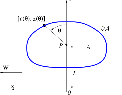
Figure 1: Schematic representation of the problem geometry in the meridional plane $(r,z)$ with a representative member of Norbury’s family of vortex rings (marked with a think blue line).

Solution of the stability problem requires a convenient representation of the boundary $\partial{\mathcal{D}}$ of the vortex ring. The intersection of the vortex region ${\mathcal{D}}$ with the meridional plane $(r,z)$, which we will denote ${\mathcal{A}}$, is shown schematically in figure 1. We consider the following general parametrization of the vortex boundary ${\mathbf{x}}(\theta)=[r(\theta),z(\theta)]^{T}$, where $\theta\in[0,2\pi]$ and $r\;:\;[0,2\pi]\rightarrow{\mathbb{R}}^{+}$, $z\;:\;[0,2\pi]\rightarrow{\mathbb{R}}$ are smooth periodic functions, which can be viewed as a mapping from a unit circle to $\partial{\mathcal{A}}$. In his original work, Norbury (1973) employed the following particular form of this parametrization adapted to solutions with the fore-and-aft symmetry and given in terms of some even periodic function $g\;:\;[0,2\pi]\rightarrow{\mathbb{R}}$

$$r(\theta) =g(\theta)\cos\theta+1,$$ (3a)

$$z(\theta) =g(\theta)\sin\theta.$$ (3b)

However, in our study we retain the more general form of the parametrization expressed in terms of two functions $r=r(\theta)$ and $z=z(\theta)$, a choice motivated by the fact that in our subsequent stability analysis we will consider boundary perturbations which break the fore-and-aft symmetry of the equilibrium configurations (in principle, such a more general representation of the vortex boundary $\partial{\mathcal{A}}$ could allow one to also capture equilibrium solutions without the fore-and-aft symmetry, but no such solutions were found). The point $P$ is defined as lying halfway between the two radial extremities of the vortex region ${\mathcal{A}}$, i.e., we have $|OP|=:L={(1/2)[r(0)+r(\pi)]}$, and, following Norbury (1973), we will normalize the problem such that $L=1$. Expressing the area of the vortex region as $|{\mathcal{A}}|=\pi L^{2}\alpha^{2}=\pi\alpha^{2}$ allows us to define the mean core radius $\alpha$. Assuming a particular reference velocity $U$, the constant in (2) can be expressed as ${\mathcal{C}}=U/(L^{2}\alpha^{2})$, such that after non-dimensionalizing the problem and noting the normalization mentioned above, this constant becomes ${\mathcal{C}}=1/\alpha^{2}$ (Norbury, 1973). This leaves $\alpha$ as the sole quantity parameterizing the solutions of system (1)–(2), and thus also implicitly determining $W$ and $\psi_{0}$. We note that as $\alpha\rightarrow 0$ the solutions of (1)–(2) approach an infinitesimally thin vortex ring, whereas for $\alpha\rightarrow\sqrt{2}$ they approach Hill’s vortex in which the region ${\mathcal{A}}$ becomes a half-disk of radius 2.

A consistent way to study the evolution and equilibria of inviscid flows with discontinuous vorticity distributions is based on the formalism of contour dynamics (Pullin, 1992). Given a time-dependent region ${\mathcal{A}}(t)$, where $t$ is time, its evolution can be studied by tracking the points ${\mathbf{y}}(t)$ on its boundary $\partial{\mathcal{A}}(t)$ via the equation

$$\frac{d{\mathbf{y}}(t)}{dt}={\mathbf{v}}({\mathbf{y}}(t)):={\mathcal{C}}\,\int_{\partial{\mathcal{A}}(t)}{\bf K}({\mathbf{y}}(t),{\mathbf{y}}^{\prime})\,ds_{{\mathbf{y}}^{\prime}},\quad\forall{\mathbf{y}}(t)\in\partial{\mathcal{A}}(t),$$ (4)

where ${\mathbf{v}}$ denotes the velocity, ${\bf K}({\mathbf{y}}(t),{\mathbf{y}}^{\prime})$ is a suitable Biot-Savart kernel, ${\mathbf{y}}$ and ${\mathbf{y}}^{\prime}$ are defined in the absolute frame of reference and $ds_{{\mathbf{y}}^{\prime}}$ is an arclength element of the vortex boundary in the meridional plane. An equilibrium shape of the vortex boundary $\partial{\mathcal{A}}$ when the right-hand side (RHS) in (1a) has a step discontinuity, cf. (2), can be characterized by transforming the coordinates to the translating frame of reference ${\mathbf{x}}(t)={\mathbf{y}}(t)-Wt\,{\mathbf{e}}_{z}$ and considering the normal component of equation (4)

$${\mathbf{n}}_{{\mathbf{x}}}\cdot\frac{d{\mathbf{x}}(t)}{dt}={\mathbf{n}}_{{\mathbf{x}}}\cdot\left[{\mathcal{C}}\,\int_{\partial{\mathcal{A}}}{\bf K}({\mathbf{x}}(t),{\mathbf{x}}^{\prime})\,ds_{{\mathbf{x}}^{\prime}}-W\,{\mathbf{e}}_{z}\right]=0,$$ (5)

where ${\mathbf{n}}_{{\mathbf{x}}}:=[n_{r},n_{z}]^{T}$ denotes the unit vector normal to the contour $\partial{\mathcal{A}}$ at the point ${\mathbf{x}}$ and directed outward. Equation (5) expresses the vanishing of the normal velocity component on the vortex boundary in relative equilibrium. Further below we will also use the unit tangent vector ${\mathbf{t}}_{{\mathbf{x}}}:=[t_{r},t_{z}]^{T}$ at the point ${\mathbf{x}}$ (we will adhere to the convention that a subscript on a geometric quantity, such as the tangent or normal vector and the curvature, will indicate where this quantity is evaluated). Since we have ${\mathbf{x}}(0)={\mathbf{y}}(0)$, the arguments of the kernel ${\bf K}$ could be changed from ${\mathbf{y}}$ and ${\mathbf{y}}^{\prime}$ in (4) to ${\mathbf{x}}$ and ${\mathbf{x}}^{\prime}$ in (5). As the equilibrium shape of the boundary $\partial{\mathcal{A}}$ is in general a priori unknown, relation (5) reveals the free-boundary aspect of the problem. The Biot-Savart kernel ${\bf K}$ appearing in (4) and (5) is obtained from the standard form of this kernel in 3D by integrating it with respect to the azimuthal angle $\phi$, which is justified by the axisymmetry assumption. As a result, in relations (4)–(5) integration needs to be performed in the meridional plane only. Expressions for such an axisymmetric Biot-Savart kernel were derived by Wakelin & Riley (1996) with an alternative, but equivalent, formulation also given by Pozrikidis (1986). Here we will use this kernel in the form rederived and tested by Shariff et al. (2008)

$${\bf K}(r\,{\mathbf{e}}_{r}+z\,{\mathbf{e}}_{z},r^{\prime}\,{\mathbf{e}}_{r}+z^{\prime}\,{\mathbf{e}}_{z})= -r^{\prime}H(r,z,r^{\prime},z^{\prime})\,n_{z}(r^{\prime},z^{\prime})\,{\mathbf{e}}_{r}$$ (6)

$$-\left[(z^{\prime}-z)\,G(r,z,r^{\prime},z^{\prime})\,n_{z}(r^{\prime},z^{\prime})-r\,H(r,z,r^{\prime},z^{\prime})\,n_{r}(r^{\prime},z^{\prime})\right]\,{\mathbf{e}}_{z},$$

where

$$G(r,z,r^{\prime},z^{\prime}) :=\frac{r^{\prime}}{\pi\sqrt{A+B}}K(\sigma),$$

$$H(r,z,r^{\prime},z^{\prime}) :=\frac{1}{2\pi r}\left[\frac{A}{\sqrt{A+B}}K(\sigma)-E(\sigma)\,\sqrt{A+B}\right]$$

in which

$$A:=r^{2}+r^{\prime 2}+(z-z^{\prime})^{2},\qquad B:=2rr^{\prime},\qquad\sigma:=\sqrt{\frac{2B}{A+B}},$$

whereas $K(\sigma)$ and $E(\sigma)$ are the complete elliptic integrals of the first and second kind, respectively (Olver et al., 2010). We note that $\sigma\rightarrow 1$ as $r^{\prime}\rightarrow r$ and $z^{\prime}\rightarrow z$, and at $\sigma=1$ the function $K(\sigma)$ has a logarithmic singularity (more details about the singularity structure of kernel (6) will be provided in §3).

Combining the kinematic condition (5) with the normalization condition $L=1$, we obtain the following system of equations defining solutions of problem (1)–(2), i.e., the vortex region ${\mathcal{A}}$ and the translation velocity $W$, as a function of the parameter (the mean core radius) $\alpha\in(0,\sqrt{2}]$

$$\frac{1}{\alpha^{2}}{\mathbf{n}}_{{\mathbf{x}}}\cdot\int_{\partial{\mathcal{A}}}{\bf K}({\mathbf{x}},{\mathbf{x}}^{\prime})\,ds_{{\mathbf{x}}^{\prime}}-W\,{\mathbf{n}}_{{\mathbf{x}}}\cdot{\mathbf{e}}_{z} =0,{\qquad\forall{\mathbf{x}}\in\partial{\mathcal{A}}}$$ (7a)

$${r(0)+r(\pi)}-2 =0,$$ (7b)

$$|{\mathcal{A}}|-\pi\alpha^{2} =0.$$ (7c)

In order to obtain his family of vortex rings, Norbury (1973) solved a system equivalent to (7) in which equation (7a) was replaced with the condition $\psi=\psi_{0}$ on $\partial{\mathcal{A}}$, where the streamfunction $\psi$ was evaluated using an integral expression involving Green’s function of the operator ${\mathcal{L}}$. He did this by representing the function $g$ in (3) in terms of a truncated cosine series and then solving the resulting discrete system using Newton’s method in which the entries of the Jacobian matrix were approximated using finite differences. The results are reported in Norbury (1973) in the form of cosine-series coefficients of the function $g$, cf. (3), obtained for different values of $\alpha\in(0,\sqrt{2})$. While in principle one could use these solutions to define the base states in our stability analysis, we will recompute the family of vortex rings to much higher precision using a method which is more accurate than Norbury’s original approach. In addition, this will also allow us to find members of this family for values of the parameter $\alpha$ not considered by Norbury (1973), which will be important for understanding exactly how the stability properties of the vortex rings vary with $\alpha$, i.e., in function of the “fatness” of the vortex rings. It is preferable to solve the problem based on formulation (7), rather than the one used originally by Norbury (1973), because in the former case the Jacobian computed with respect to the shape of the contour $\partial{\mathcal{A}}$ can be reused in a straightforward manner for the stability calculations. Below we present a brief outline of this approach.

The idea of the approach is to find a deformation of some initial reference contour such that conditions (7a)–(7c) are satisfied. System (7) is solved, in a suitable discretized form, using Newton’s method in which the required contour deformation (Newton’s step) is found approximately by solving a linear system (Jacobian) obtained by differentiating (7) with respect to the shape of the contour $\partial{\mathcal{A}}$. Taking ${\mathbf{x}}$ to represent the contour approximating the vortex boundary $\partial{\mathcal{A}}$ at a certain iteration, its perturbation ${\mathbf{x}}^{\epsilon}$ obtained by applying a small but otherwise arbitrary deformation can be described as

$${\mathbf{x}}^{\epsilon}(\theta)={\mathbf{x}}(\theta)+\epsilon\,\rho(\theta)\,{\mathbf{n}}_{{\mathbf{x}}(\theta)},$$ (8)

where $\epsilon>0$ and $\rho\;:\;[0,2\pi]\rightarrow{\mathbb{R}}$ is a periodic function describing the shape of the perturbation. We will adopt the convention that the superscript $\epsilon$ will denote quantities corresponding to the perturbed boundary, so that ${\mathbf{x}}={\mathbf{x}}^{\epsilon}|_{\epsilon=0}$ and ${\mathbf{n}}_{{\mathbf{x}}}={\mathbf{n}}_{{\mathbf{x}}^{\epsilon}}|_{\epsilon=0}$ are the quantities corresponding to the reference shape. Since an arbitrary contour $\partial{\mathcal{A}}$ does not represent an equilibrium, system (7) defining the equilibrium can be equivalently expressed as the following conditions on the deformation $\rho$ and the translation velocity $W$ obtained by setting $\epsilon=1$ in ansatz (8)

$$F\left(\begin{bmatrix}\rho\\ W\end{bmatrix}\right):=\begin{bmatrix}{{\mathbf{n}}_{{\mathbf{x}}(\theta)+\rho(\theta)\,{\mathbf{n}}_{{\mathbf{x}}(\theta)}}\cdot{\mathbf{v}}({\mathbf{x}}(\theta)+\rho(\theta)\,{\mathbf{n}}_{{\mathbf{x}}(\theta)})-W\,{\mathbf{n}}_{{\mathbf{x}}(\theta)+\rho(\theta)\,{\mathbf{n}}_{{\mathbf{x}}(\theta)}}\cdot{\mathbf{e}}_{z}}\\ {\left[r(0)+\rho(0)\,n_{r}(0)\right]+\left[r(\pi)+\rho(\pi)\,n_{r}(\pi)\right]-2}\\ {|{\mathcal{A}}(\rho)|}-\pi\alpha^{2}\end{bmatrix}=\begin{bmatrix}0\\ 0\\ 0\end{bmatrix},$$ (9)

where the first component of $F$ is to be interpreted as a relation holding for all $\theta\in[0,2\pi]$ and $|{\mathcal{A}}(\rho)|$ is the area inside the perturbed contour. Infinite-dimensional (continuous) system (9) can be converted to an algebraic form amenable to numerical solution with Newton’s method by discretizing the parameter $\theta$ uniformly as $\theta_{j}=(j-1)\Delta\theta$, $j=1,\dots,M$, where $\Delta\theta=2\pi/M$ and $M$ is an even integer. The perturbation $\rho(\theta)$ is approximated in terms of a truncated Fourier series

$$\rho(\theta)\approx\rho_{N}(\theta):=\sum_{k=0}^{N}a_{k}\cos(k\theta)+\sum_{k=1}^{N}b_{k}\sin(k\theta),$$ (10)

where $N:=M/2$. The cosine- and sine-series coefficients of the shape perturbation $\rho_{N}$ can then be combined into a vector

$${\mathbf{z}}=\left[a_{0},a_{1},\dots,a_{N},b_{1},\dots,b_{N}\right]^{T}\in{\mathbb{R}}^{M+1}.$$ (11)

After collocating the first component of (9), cf. (7a), at the discrete parameter values $\theta_{j}$, $j=1,\dots,M$, and using suitable discretizations (to be described below), the resulting algebraic system takes the form

$${\bf F}\left(\begin{bmatrix}{\mathbf{z}}\\ W\end{bmatrix}\right)=\begin{bmatrix}\mathbf{0}\\ 0\\ 0\end{bmatrix},$$ (12)

where ${\bf F}\;:\;{\mathbb{R}}^{M+2}\rightarrow{\mathbb{R}}^{M+2}$ and $\mathbf{0}\in{\mathbb{R}}^{M}$ is a column vector of zeros. Relation (12) represents a system of nonlinear algebraic equations which can be solved using Newton’s method. Denoting $\boldsymbol{\Delta}{\mathbf{z}}$ and $\Delta W$ the components of Newton’s step corresponding to the updates, respectively, of the series coefficients (11) of the shape perturbation and of the translation velocity $W$, a single iteration of Newton’s method requires solution of the system

$$\boldsymbol{\nabla}{\bf F}\left(\begin{bmatrix}{\mathbf{z}}\\ W\end{bmatrix}\right)\begin{bmatrix}\boldsymbol{\Delta}{\mathbf{z}}\\ \Delta W\end{bmatrix}=-{\bf F}\left(\begin{bmatrix}{\mathbf{z}}\\ W\end{bmatrix}\right),$$ (13a)

$$\text{where}\quad\boldsymbol{\nabla}{\bf F}\left(\begin{bmatrix}{\mathbf{z}}\\ W\end{bmatrix}\right):=\begin{bmatrix}\left({\bf M}-W\operatorname{diag}\left({\mathbf{e}}_{z}\cdot{\mathbf{t}}_{{\mathbf{x}}(\theta_{1},\dots,\theta_{M})}\right)\boldsymbol{\Xi}\right)&\left({\mathbf{e}}_{z}\cdot{\mathbf{n}}_{{\mathbf{x}}(\theta_{1},\dots,\theta_{M})}\right)\\ -[0,2,\dots,0,2][0,\dots,0]&0\\ \left[U_{0},U_{1},\dots,U_{N},V_{1},\dots,V_{N}\right]&0\end{bmatrix}$$ (13b)

is the Jacobian of the function ${\bf F}$, cf. (12), in which the expressions in the first column represent the partial derivatives of the discretized kinematic condition (7a), the normalization condition (7b) and the fixed-area condition (7c) with respect to the expansion coefficients (11) obtained using methods of the shape calculus (Delfour & Zolésio, 2001), cf. §3, whereas the expressions in the second column are the partial derivatives of these conditions with respect to the translation velocity $W$. The vectors in the first row are to be understood as ${\mathbf{e}}_{z}\cdot{\mathbf{t}}_{{\mathbf{x}}(\theta_{1},\dots,\theta_{M})}:=[t_{z}(\theta_{1}),\dots,t_{z}(\theta_{M})]^{T}$ and ${\mathbf{e}}_{z}\cdot{\mathbf{n}}_{{\mathbf{x}}(\theta_{1},\dots,\theta_{M})}:=[n_{z}(\theta_{1}),\dots,n_{z}(\theta_{M})]^{T}$. Since the matrix ${\bf M}$ also arises in the discretization of the stability problem, evaluation of its entries is discussed in detail in §4, cf. (51). The term $W\operatorname{diag}\left({\mathbf{e}}_{z}\cdot{\mathbf{t}}_{{\mathbf{x}}(\theta_{1},\dots,\theta_{M})}\right)\boldsymbol{\Xi}$, where the matrix $\boldsymbol{\Xi}$ is defined in (35), results from shape differentiation of the second term on the left-hand side (LHS) in condition (7a). Noting that the shape differential of the vortex area $|{\mathcal{A}}(\rho)|$ is $|{\mathcal{A}}(\rho)|^{\prime}=\left(\int_{{\mathcal{A}}}\,d{\mathcal{A}}\right)^{\prime}=\int_{\partial{\mathcal{A}}}\rho\,ds$ (Delfour & Zolésio, 2001), the partial derivatives of the fixed-area condition (7c) with respect to expansion coefficients (11) are obtained as $U_{k}:=\int_{0}^{2\pi}\cos(k\theta^{\prime})\frac{ds}{d\theta}(\theta^{\prime})\,d\theta^{\prime}$, $V_{k}:=\int_{0}^{2\pi}\sin(k\theta^{\prime})\frac{ds}{d\theta}(\theta^{\prime})\,d\theta^{\prime}$, $k=0,\dots,M$, where $s(\theta)$ is the arclength of the contour. Details concerning a spectrally-accurate approach to evaluate such expressions are provided in §4.

The Jacobian $\boldsymbol{\nabla}{\bf F}$ in (13b) is singular with a one-dimensional kernel space corresponding to arbitrary shifts of the contour $\partial{\mathcal{A}}$ in the $z$ direction. In the process of solving (13a) to compute Newton’s step the singular-value decomposition (SVD) is used to ensure that the obtained Newton’s step is orthogonal to this subspace.

We emphasize that, as will be evident in §3, the Jacobian $\boldsymbol{\nabla}{\bf F}$ also contains key information necessary to set up the generalized eigenvalue problem for the study of the stability of vortex rings with respect to axisymmetric perturbations. This fact constitutes the main practical advantage of the approach developed here with respect to the method originally devised by Norbury (1973). Since the vortex rings are known to possess a fore-and-aft symmetry, in ansatz (10) only the cosine-series coefficients will be nonzero, i.e., $b_{1}=\dots=b_{N}=0$, leading, via relation (8), to functions $r(\theta)$ and $z(\theta)$ which are, respectively, even and odd. However, we retain the sine series in subsequent derivations, because their outcomes will be also used in the stability analysis in §3 where general perturbations without the fore-and-aft symmetry will be considered.

Since for all $\alpha\in(0,\sqrt{2})$ the contours $\partial{\mathcal{A}}$ are smooth (Norbury, 1973), we can expect spectral convergence of the expansion (10), i.e., $|a_{k}|\sim e^{-\beta k}$ for $k\rightarrow\infty$ and some $\beta>0$ (Trefethen, 2013). However, since the kinematic condition (7a) involves a convolution integral which is discretized using a collocation approach, one may expect that aliasing errors will arise (Boyd, 2001). They will manifest themselves through an increase of $|a_{k}|$ with $k$ when $k>k_{a}$ for a certain $k_{a}>0$. This issue is efficiently remedied by using an implicit filtering approach in which Newton’s step (13a) is redefined as

$$\boldsymbol{\nabla}{\bf F}\left(\begin{bmatrix}{\mathbf{z}}\\ W\end{bmatrix}\right)\begin{bmatrix}{\bf G}^{\delta}\boldsymbol{\Delta}{\mathbf{z}}\\ \Delta W\end{bmatrix}=-{\bf F}\left(\begin{bmatrix}{\mathbf{z}}\\ W\end{bmatrix}\right)$$ (14)

in which ${\bf G}^{\delta}\in{\mathbb{R}}^{(M+1)\times(M+1)}$ is a smoothing operator given by a low-pass filter, here represented by the following diagonal matrix

$${\bf G}^{\delta}:=\operatorname{diag}\left(0,\left[\frac{1}{1+(\delta k)^{2p}},\ k=1,\dots,M\right],\left[\frac{1}{1+(\delta k)^{2p}},\ k=1,\dots,M\right]\right).$$ (15)

In computations we will take $p=4$ as the order of the filter, whereas the cutoff length-scale $\delta$ will be refined with the resolution $M$ as $\delta=2\pi\gamma/M$ for some $\gamma>1$ ensuring that filtering does not affect the spectral accuracy of the approach.

As the vortex rings become “fatter” in the limit $\alpha\rightarrow\sqrt{2}$, the shape of their boundary $\partial A$ deviates from the circle and develops “corners” characterized by an increasing curvature. In order to resolve these features, increased resolutions must be used varying from $M=32$ when $\alpha=0.1$ to $M=4096$ when $\alpha=1.4$. We have carefully checked the convergence of the computed shapes of the vortex boundary $\partial{\mathcal{A}}$ and of the translation velocity $W$ with refinement of the resolution $M$. The iterations of Newton’s method are initiated with Norbury’s original solutions documented in Norbury (1973), or with neighboring solutions for values of $\alpha$ not considered by Norbury (1973). The iterations are declared converged when the following stringent termination conditions are simultaneously satisfied

$$\Bigg{|}\Bigg{|}{\bf F}\left(\begin{bmatrix}{\mathbf{z}}\\ W\end{bmatrix}\right)\Bigg{|}\Bigg{|}_{2}<\widetilde{\varepsilon}\quad\text{and}\quad\Bigg{|}\Bigg{|}{\bf F}\left(\begin{bmatrix}{\mathbf{z}}\\ W\end{bmatrix}\right)\Bigg{|}\Bigg{|}_{\infty}<\widetilde{\varepsilon},$$ (16)

where the tolerance was set as $\widetilde{\varepsilon}=10^{-10}$ for $\alpha\in(0,1.2]$ and was gradually relaxed to $\widetilde{\varepsilon}=10^{-5}$ as $\alpha$ increased to 1.4. The reason for relaxing the tolerance is that at higher resolutions required to represent the shapes of the vortex boundary when $\alpha>1.2$, the accuracy of the solution is ultimately limited by the poor algebraic conditioning of the (desingularized) Jacobian matrix (13b). More specifically, the value of $\widetilde{\varepsilon}$ roughly reflects the accuracy with which Newton’s step $\left[{\bf G}^{\delta}\boldsymbol{\Delta}{\mathbf{z}}^{T},\Delta W\right]^{T}$ can be evaluated by solving problem (14) at a given resolution. In all cases convergence was typically achieved in $\mathcal{O}(10)$ iterations, although due to the singularity of the Jacobian (13b) convergence was only linear. In the cases when Norbury’s original solutions were used as the initial guesses, the residuals (16) would typically decrease by 8–10 orders of magnitude.

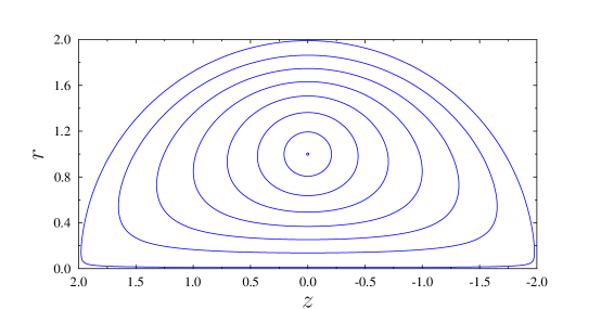
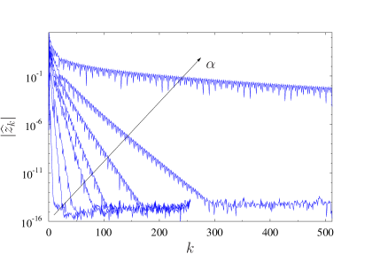
Figure 2: (a) Vortex boundaries $\partial{\mathcal{A}}$ obtained by solving system (12) for $\alpha=0.01,0.2,0.4,0.6,0.8,1.0,1.2,1.4$. (b) The amplitudes of the Fourier coefficients $\widehat{x}_{k}$, $k=1,\dots,N$, of the corresponding parametrizations $r(\theta)$ obtained for the same values of $\alpha$ (the trend with the increase of $\alpha$ is indicated with an arrow). The resolutions used in the computations varied from $N=16$ for small $\alpha$ to $N=2048$ for $\alpha\rightarrow\sqrt{2}$.

The shapes of the vortex boundary $\partial{\mathcal{A}}$ obtained as solutions to (12) for representative values of $\alpha$ are presented in figure 2(a) where a gradual evolution of the shape from a thin vortex filament to Hill’s “fat” vortex is evident as $\alpha$ increases from 0.01 to nearly $\sqrt{2}$. To simplify notation, hereafter the equilibrium shapes of the vortex boundary $\partial{\mathcal{A}}$ are denoted ${\mathbf{x}}=[r,z]^{T}$, with the coordinates given in terms of parametrizations $r=r(\theta)$ and $z=z(\theta)$. The amplitudes of the corresponding Fourier coefficients $\widehat{z}_{k}$, $k=1,\dots,N$, are shown in figure 2(b) (the spectra of $r(\theta)$ are essentially indistinguishable and are not shown). We see that for all values of $\alpha$ the amplitudes $|\widehat{z}_{k}|$ of the Fourier coefficients decay exponentially with the wavenumber $k$, although this property is gradually lost as $\alpha\rightarrow\sqrt{2}$ where the vortex boundary $\partial{\mathcal{A}}$ develops a sharp corner (such that $r(\theta)$ and $z(\theta)$ are no longer smooth functions of $\theta$). In figure 2(b) we also observe that, interestingly, the dependence of $|\widehat{z}_{k}|$ on the wavenumber $k$ is characterized by a certain recurrent pattern. The translation velocity $W$ is positive for all values of $\alpha$, meaning that the vortices shown in figure 2(a) move to the left. When $\alpha\rightarrow 0$, this translation velocity becomes unbounded as $(1/4)(\ln(8/\alpha)-1/4)$, whereas when $\alpha\rightarrow\sqrt{2}$, $W$ approaches $4/15$, both of which are well-known results for the propagation velocity of an infinitely thin vortex ring and Hill’s vortex, respectively (Wu et al., 2006). As regards the integral diagnostics, the variation of the vortex area $|{\mathcal{A}}|$, its circulation $\Gamma$ and its hydrodynamic impulse ${\mathcal{I}}$ with $\alpha$ is consistent with the behavior of these quantities discussed in Norbury (1973), both as $\alpha\rightarrow 0$ and $\alpha\rightarrow\sqrt{2}$. The data $\{r_{j},z_{j}\}$, where $r_{j}=r(\theta_{j})$ and $z_{j}=z(\theta_{j})$, $j=1,\dots,M$, describing the vortex boundaries $\partial{\mathcal{A}}$ for a range of different $\alpha\in(0,\sqrt{2})$ is provided in Supplementary Information together with the corresponding values of the propagation velocity $W$. The linear stability of these equilibrium configurations is discussed in the next section.

3 Linear Stability Analysis

In this section we derive a singular integro-differential equation characterizing the linear response of the boundary $\partial{\mathcal{A}}(t)$ of Norbury’s vortices, cf. figure 2(a), to axisymmetric perturbations. This will be done by applying the tools of the shape-differential calculus (Delfour & Zolésio, 2001) to the contour-dynamics formulation (4) of the problem. Finally, we obtain a constrained eigenvalue problem from which the stability properties of Norbury’s vortices can be deduced.

In addition to the circulation, impulse and energy conserved by all classical solutions of Euler’s equations, axisymmetric inviscid flows also conserve Casimirs $\iint_{{\mathcal{A}}(t)}\Psi({\omega}/{r})\,r\,d{\mathcal{A}}$, where $\Psi\;:\;{\mathbb{R}}\rightarrow{\mathbb{R}}$ is an arbitrary function with sufficient regularity (Mohseni, 2001). Since circulation is a particularly simple Casimir, defined by $\Psi(\xi)=\xi$ for some $\xi\in{\mathbb{R}}$, we will focus on stability analysis with respect to perturbations preserving this quantity, which is the same approach as was also taken by Moffatt & Moore (1978); Protas & Elcrat (2016) in their studies of the stability of Hill’s vortex. By this we mean that the perturbed vortex ring will have the same circulation as the corresponding vortex ring in the equilibrium configuration (however, under the linearized Euler evolution, this circulation will in general change). The circulation $\Gamma$ of the flow in the meridional plane is defined as

$$\Gamma:=\iint_{{\mathcal{A}}(t)}{\omega}\,d{\mathcal{A}}$$ (17)

and, since the flows considered here have the property $\omega={\mathcal{C}}r$, cf. (1)–(2), conservation of circulation (17) implies the conservation of the volume of the vortical region. We add that restricting the vorticity of the perturbed vortex to the form $\omega={\mathcal{C}}r$ is justified by recognizing that such configurations can be obtained as rearrangements of the vorticity distribution in the reference configuration (Brooke Benjamin, 1975).

We now describe how axisymmetric perturbations are applied to the equilibrium configurations discussed in §2, cf. figure 2(a). Following the ideas laid out by Elcrat & Protas (2013), we now assume that the position of the vortex boundary $\partial{\mathcal{A}}(t)$ depends on time $t$ and, to simplify calculations, introduce another parametrization ${\mathbf{x}}={\mathbf{x}}(t,s)\in\partial{\mathcal{A}}(t)$ for it, now in terms of the arclength $s$ of the contour. Since the maps $r=r(\theta)$ and $z=z(\theta)$ are assumed invertible and $ds=\sqrt{(dr)^{2}+(dx)^{2}}$, we can rewrite ansatz (8) as

$${\mathbf{x}}^{\epsilon}(t,s)={\mathbf{x}}(s)+\epsilon\,\rho(t,s)\,{\mathbf{n}}_{{\mathbf{x}}(s)},$$ (18)

where $s=s(\theta)$ and the point ${\mathbf{x}}$ belongs to the boundary $\partial{\mathcal{A}}$ of the equilibrium configuration. We remark that for smooth reference contours ${\mathbf{x}}$ ansatz (18) does not restrict the class of admissible contour deformations except for the assumption that the perturbed contour ${\mathbf{x}}^{\epsilon}$ be “close” to the reference contour ${\mathbf{x}}$ (Delfour & Zolésio, 2001), which is however consistent with how the linear stability problem is formulated. Using equation (4) we then deduce

$${\mathbf{n}}_{{\mathbf{x}}^{\epsilon}}\cdot\frac{d{\mathbf{x}}^{\epsilon}(t)}{dt}={{\mathbf{n}}_{{\mathbf{x}}^{\epsilon}}\cdot}{\mathbf{v}}^{\epsilon}({\mathbf{x}}^{\epsilon}(t))={\mathbf{n}}_{{\mathbf{x}}^{\epsilon}}\cdot\left[{\mathcal{C}}\,\int_{\partial{\mathcal{A}}^{\epsilon}(t)}{\bf K}({\mathbf{x}}^{\epsilon}(t),{\mathbf{x}}^{\prime})\,ds_{{\mathbf{x}}^{\prime}}-W\,{\mathbf{e}}_{z}\right],$$ (19)

from which the equilibrium condition (5) is obtained by setting $\epsilon=0$. The equation describing the evolution of the perturbation $\rho$ is obtained by linearizing relation (19) around the equilibrium configuration characterized by (5) which is equivalent to expanding (19) in powers of $\epsilon$ and retaining the first-order terms. Since equation (19) involves perturbed quantities defined on the perturbed vortex boundary $\partial A^{\epsilon}(t)$, the proper way to obtain this linearization is using methods of the shape-differential calculus (Delfour & Zolésio, 2001). Below we state the main results only and refer the reader to our earlier study (Elcrat & Protas, 2013) for details of all intermediate transformations. Shape-differentiating the left-hand side of relation (19) and setting $\epsilon=0$ we obtain

$$\frac{d}{d\epsilon}\left[{\mathbf{n}}_{{\mathbf{x}}^{\epsilon}}\cdot\frac{d{\mathbf{x}}^{\epsilon}(t)}{dt}\right]\bigg{|}_{\epsilon=0}={\partial\rho\over\partial t}.$$ (20)

As regards the right-hand side (RHS) in (19), we obtain

$$\frac{d}{d\epsilon}\left\{{\mathbf{n}}_{{\mathbf{x}}^{\epsilon}}\cdot\left[{\mathcal{C}}\,\int_{\partial{\mathcal{A}}^{\epsilon}(t)}{\bf K}({\mathbf{x}}^{\epsilon}(t),{\mathbf{x}}^{\prime})\,ds_{{\mathbf{x}}^{\prime}}-W\,{\mathbf{e}}_{z}\right]\right\}\Bigg{|}_{\epsilon=0}=\\ =-{\partial\rho\over\partial s}\,{\mathbf{v}}({\mathbf{x}})\cdot{\mathbf{t}}_{{\mathbf{x}}}+{\mathcal{C}}\,\rho(s)\,{\mathbf{n}}_{{\mathbf{x}}}\cdot\int_{\partial{\mathcal{A}}}{\partial{\bf K}\over\partial n_{{\mathbf{x}}}}\,ds^{\prime}+{\mathcal{C}}\,{\mathbf{n}}_{{\mathbf{x}}}\cdot\int_{\partial{\mathcal{A}}}{\bf K}^{\prime}+\left[{\partial{\bf K}\over\partial n_{{\mathbf{x}}^{\prime}}}+\varkappa_{{\mathbf{x}}^{\prime}}{\bf K}\right]\rho(s^{\prime})\,ds^{\prime},$$ (21)

where $\varkappa_{{\mathbf{x}}}$ is the curvature of the contour $\partial{\mathcal{A}}$ and ${\bf K}^{\prime}$ is the shape differential of the kernel ${\bf K}$, cf. (6). The orientation of the unit vectors ${\mathbf{t}}_{{\mathbf{x}}}$ and ${\mathbf{n}}_{{\mathbf{x}}}$, and the sign of the curvature $\varkappa_{{\mathbf{x}}}$ satisfy Frenet’s convention. The terms in the integrand expressions in (21) involving the derivatives of the kernel in the directions of the normal vectors are expressed as $\partial{\bf K}/\partial n_{{\mathbf{x}}}={\mathbf{n}}_{{\mathbf{x}}}\cdot\boldsymbol{\nabla}_{{\mathbf{x}}}{\bf K}({\mathbf{x}},{\mathbf{x}}^{\prime})$ and $\partial{\bf K}/\partial n_{{\mathbf{x}}^{\prime}}={\mathbf{n}}_{{\mathbf{x}}^{\prime}}\cdot\boldsymbol{\nabla}_{{\mathbf{x}}^{\prime}}{\bf K}({\mathbf{x}},{\mathbf{x}}^{\prime})$, where the subscript on the operator $\boldsymbol{\nabla}$ indicates which variable differentiation is performed with respect to, whereas the shape differential of the kernel is evaluated as follows

$${\bf K}^{\prime}(r,z,r^{\prime},z^{\prime}) =-r^{\prime}H(r,z,r^{\prime},z^{\prime})\,\frac{d}{d\epsilon}n^{\epsilon}_{z}(r^{\prime},z^{\prime})\big{|}_{\epsilon=0}\,{\mathbf{e}}_{r}$$ (22)

$$\phantom{=}-\left[(z^{\prime}-z)\,G(r,z,r^{\prime},z^{\prime})\,\frac{d}{d\epsilon}n^{\epsilon}_{z}(r^{\prime},z^{\prime})\big{|}_{\epsilon=0}-r\,H(r,z,r^{\prime},z^{\prime})\,\frac{d}{d\epsilon}n^{\epsilon}_{r}(r^{\prime},z^{\prime})\big{|}_{\epsilon=0}\right]\,{\mathbf{e}}_{z}$$

$$=r^{\prime}H(r,z,r^{\prime},z^{\prime})\,n_{r}(r^{\prime},z^{\prime})\,{\partial\rho\over\partial s}\,{\mathbf{e}}_{r}$$

$$\phantom{=}+\left[(z^{\prime}-z)\,G(r,z,r^{\prime},z^{\prime})\,n_{r}(r^{\prime},z^{\prime})+r\,H(r,z,r^{\prime},z^{\prime})\,n_{x}(r^{\prime},z^{\prime})\right]\,{\partial\rho\over\partial s}\,{\mathbf{e}}_{z}$$

$$=:{\bf DK}^{\prime}(r,z,r^{\prime},z^{\prime})\,{\partial\rho\over\partial s},$$

where the second equality follows from the expression for the shape derivative of the unit normal vector, i.e., $d{\mathbf{n}}^{\epsilon}/d\epsilon\,|_{\epsilon=0}=-(\partial\rho/\partial s)\,{\mathbf{t}}$, and Frenet’s identities (Elcrat & Protas, 2013).

As explained by Elcrat & Protas (2013), the three terms on the RHS of (21) represent the shape-sensitivity of the RHS of (19) to perturbations (18) applied separately to the normal vector ${\mathbf{n}}_{{\mathbf{x}}}$, the evaluation point ${\mathbf{x}}$ and the contour $\partial{\mathcal{A}}$ over which the integral is defined. Since the flow evolution is subject to constraint (17), this will restrict the admissible perturbations $\rho$. Indeed, noting that $\omega={\mathcal{C}}r$, cf. (1)–(2), and shape-differentiating relation (17) we obtain the following condition (Elcrat & Protas, 2013)

$$\int_{\partial{\mathcal{A}}}{{r}\rho(0,s^{\prime})}\,ds^{\prime}=0$$ (23)

restricting the class of admissible perturbations to those which do not modify the circulation (17) (analogous conditions can be obtained when the perturbations are constructed to preserve other integral invariants mentioned above). We note that the constraint imposed in the formulation of the stability problem, cf. (17), is different from the constraints which were imposed during the computation of the equilibrium configurations, cf. (7b)–(7c), which resulted from the assumed normalization.

It is now convenient to return to the original parametrization in terms of $\theta$, i.e., assume again that $r=r(\theta)$, $z=z(\theta)$, $r^{\prime}=r^{\prime}(\theta^{\prime})$ and $z^{\prime}=z^{\prime}(\theta^{\prime})$, such that combining relations (20)–(23) and replacing the line integrals with the corresponding definite ones we finally obtain the equation describing the deformation $\rho(t,\theta)$ of the vortex boundary $\partial{\mathcal{A}}(t)$, cf. (18), in response to axisymmetric perturbations in the linear regime

$${\partial\rho\over\partial t} =-{\mathcal{C}}\,{\partial\rho\over\partial\theta}\left(\frac{ds}{d\theta}\right)^{-1}\,\int_{0}^{2\pi}I_{0}(\theta,\theta^{\prime})\frac{ds}{d\theta}(\theta^{\prime})\,d\theta^{\prime}+{\mathcal{C}}\,\rho(\theta)\,\int_{0}^{2\pi}I_{1}(\theta,\theta^{\prime})\frac{ds}{d\theta}(\theta^{\prime})\,d\theta^{\prime}$$

$$\phantom{=}+{\mathcal{C}}\,\int_{0}^{2\pi}I_{2}(\theta,\theta^{\prime})\rho(\theta^{\prime})\frac{ds}{d\theta}(\theta^{\prime})\,d\theta^{\prime}+{\mathcal{C}}\,\int_{0}^{2\pi}I_{3}(\theta,\theta^{\prime}){\partial\rho\over\partial\theta}(\theta^{\prime})\,d\theta^{\prime}$$ (24a)

$$=:\left({{\mathcal{G}}}\rho\right)(\theta)$$

$$\textrm{subject to:}\quad\int_{0}^{2\pi}r(\theta^{\prime})\rho(\theta^{\prime})\frac{ds}{d\theta}(\theta^{\prime})\,d\theta^{\prime}=0,$$ (24b)

where ${\mathcal{G}}$ denotes the associated linear operator and

$$I_{0}(\theta,\theta^{\prime}) :={\mathbf{t}}_{\theta}\cdot{\bf K}(\theta,\theta^{\prime}),$$ (25a)

$$I_{1}(\theta,\theta^{\prime}) :={\mathbf{n}}_{\theta}\cdot{\partial{\bf K}(\theta,\theta^{\prime})\over\partial n_{\theta}},$$ (25b)

$$I_{2}(\theta,\theta^{\prime}) :={\mathbf{n}}_{\theta}\cdot\left[{\partial{\bf K}(\theta,\theta^{\prime})\over\partial n_{\theta^{\prime}}}+\varkappa_{\theta^{\prime}}{\bf K}(\theta,\theta^{\prime})\right],$$ (25c)

$$I_{3}(\theta,\theta^{\prime}) :={\mathbf{n}}_{\theta}\cdot{\bf DK}(\theta,\theta^{\prime}).$$ (25d)

Given the form of the kernel ${\bf K}$, cf. (6), expressions (25a)–(25d) take rather complicated forms as functions of $r(\theta)$, $z(\theta)$, $r^{\prime}(\theta^{\prime})$, and $z^{\prime}(\theta^{\prime})$. They can be however readily obtained using symbolic algebra tools such as Maple.

As regards the singularities of the kernels, one can verify by inspection that

$$\forall\ \theta,\theta^{\prime}\in[0,2\pi]\quad \lim_{\theta^{\prime}\rightarrow\theta}\,{\mathbf{n}}_{\theta}\cdot{\bf K}(\theta,\theta^{\prime})=0,$$ (26a)

$$\lim_{\theta^{\prime}\rightarrow\theta}\,\frac{I_{0}(\theta,\theta^{\prime})}{\ln\sin^{2}\left(\frac{\theta-\theta^{\prime}}{2}\right)}=-\frac{1}{4\pi}r(\theta),$$ (26b)

$$\lim_{\theta^{\prime}\rightarrow\theta}\,\frac{I_{1}(\theta,\theta^{\prime})}{\ln\sin^{2}\left(\frac{\theta-\theta^{\prime}}{2}\right)}=-\frac{1}{4\pi}n_{z}(\theta),$$ (26c)

$$\lim_{\theta^{\prime}\rightarrow\theta}\,\frac{I_{2}(\theta,\theta^{\prime})}{\ln\sin^{2}\left(\frac{\theta-\theta^{\prime}}{2}\right)}=\frac{1}{4\pi}n_{z}(\theta),$$ (26d)

$$\lim_{\theta^{\prime}\rightarrow\theta}\,\frac{I_{3}(\theta,\theta^{\prime})}{\ln\sin^{2}\left(\frac{\theta-\theta^{\prime}}{2}\right)}=-\frac{1}{4\pi}r(\theta),$$ (26e)

where the expression in the denominators on the LHS is chosen to combine the correct singular behavior for $\theta^{\prime}\rightarrow\theta$ with $2\pi$-periodic dependence on $\theta$ and $\theta^{\prime}$. Relations (26b)–(26e) are deduced using known properties of the complete elliptic integrals appearing in (6) (Olver et al., 2010), and then computing the limits symbolically using the software package Maple. From (26a) we conclude that the singularity of the normal component of the kernel ${\bf K}$ is removable, whereas all the integrals in (24a) are to be understood in the improper sense. Properties (26b)–(26e) will be instrumental in achieving spectral accuracy in the discretization of system (24).

After introducing the ansatz

$${\rho(t,\theta)=e^{i\lambda t}\,u(\theta)+C.C.,}$$ (27)

where $i:=\sqrt{-1}$ and $\lambda\in{\mathbb{C}}$, system (24) takes the form of a constrained eigenvalue problem

$$i\,\lambda\,u(\theta)=\left({\mathcal{G}}u\right)(\theta), \theta\in[0,2\pi]$$ (28a)

$$\textrm{subject to:}\quad\text{periodic boundary conditions},$$ (28b)

$$\phantom{\textrm{subject to:}}\quad\int_{0}^{2\pi}r(\theta^{\prime})\rho(\theta^{\prime})\frac{ds}{d\theta}(\theta^{\prime})\,d\theta^{\prime}=0,$$ (28c)

where the operator ${\mathcal{G}}$ is defined in (24a). The eigenvalues $\lambda$ and the corresponding eigenvectors $u$ characterize the stability of Norbury’s vortex rings, cf. figure 2(a), to axisymmetric perturbations. Our approach to the numerical solution of the constrained eigenvalue problem (28) is presented in the next section.

4 Numerical Approach

In this section we describe our numerical approach focusing on the discretization of system (28) and the solution of the resulting algebraic eigenvalue problem. We will also provide some details about how these techniques have been validated. Our approach is an adaptation to the present problem of the methodology validated and thoroughly tested in earlier studies (Elcrat & Protas, 2013; Protas & Elcrat, 2016). It also shares a number of key ingredients with the methodology employed to approximate Newton’s step (13a) in the solution of problem (9) when computing equilibrium configurations in §2.

As a starting point, we recall that the equilibrium configurations of the vortex boundary $\partial{\mathcal{A}}$ are represented in terms of the parametrization $[r(\theta),z(\theta)]$, $\theta\in[0,2\pi]$, discretized (with spectral accuracy) as $\{r_{j},z_{j}\}$, $j=1,\dots,M$. The eigenvectors $u$ are then approximated with a truncated series similar to the one already used in (10), i.e.,

$$u(\theta)\approx u_{N}(\theta):=\sum_{k=0}^{N}a_{k}\cos(k\theta)+\sum_{k=1}^{N-1}b_{k}\sin(k\theta)$$ (29)

(without the risk of confusion, the expansion coefficients in (10) and (29) are denoted with the same symbols). Since the total number of coefficients parameterizing $u_{N}(\theta)$ in (29) must be equal to $M=2N$, we arbitrarily choose to truncate the sine series in (29) at $k=N-1$. After substitution of ansatz (29), equation (28a) is collocated on the uniform grid $\theta_{1},\dots\theta_{M}$, whereas constraint (28c) takes the form

$$a_{0}\,\int_{0}^{2\pi}r(\theta^{\prime})\frac{ds}{d\theta}(\theta^{\prime})\,d\theta^{\prime} +\sum_{k=1}^{N}a_{k}\,\int_{0}^{2\pi}r(\theta^{\prime})\cos(k\theta^{\prime})\frac{ds}{d\theta}(\theta^{\prime})\,d\theta^{\prime}$$ (30)

$$+\sum_{k=1}^{N-1}b_{k}\,\int_{0}^{2\pi}r(\theta^{\prime})\sin(k\theta^{\prime})\frac{ds}{d\theta}(\theta^{\prime})\,d\theta^{\prime}=0.$$

The factor $ds/d\theta=\sqrt{\left(dr(\theta)/d\theta\right)^{2}+\left(dz(\theta)/d\theta\right)^{2}}$ can be approximated at the collocation points $\theta_{j}$, $j=1,\dots,M$, as $\widetilde{ds/d\theta}|_{j}$ with spectral accuracy applying a suitable differentiation matrix for periodic functions (Trefethen, 2000) to the discrete representations of the parametrizations $r(\theta)$ and $z(\theta)$. Approximating the integrals in (30) using the trapezoidal quadrature, which for smooth integrand expressions defined on periodic domains achieves spectral accuracy, we obtain the constraint vector ${\mathbf{c}}=[c_{1},\dots,c_{M}]$, where

$$c_{1}:=\Delta\theta\sum_{j=1}^{M}r_{j}\widetilde{\frac{ds}{d\theta}}\Big{|}_{j},\quad c_{1+k} :=\Delta\theta\sum_{j=1}^{M}r_{j}\cos(k\theta^{\prime}_{j})\widetilde{\frac{ds}{d\theta}}\Big{|}_{j},\quad k=1,\dots,N,$$ (31)

$$c_{N+1+k} :=\Delta\theta\sum_{j=1}^{M}r_{j}\sin(k\theta^{\prime}_{j})\widetilde{\frac{ds}{d\theta}}\Big{|}_{j},\quad k=1,\dots,N-1.$$

We also introduce the notation ${\mathbf{w}}=[w_{1},\dots,w_{M}]^{T}$, where $w_{1}:=a_{0}$, $w_{1+k}:=a_{k}$, $k=1,\dots,N$, and $w_{N+1+k}:=b_{k}$, $k=1,\dots,N-1$. As a result, we obtain the following discretization of the generalized eigenvalue problem (28)

$$i\lambda\sum_{k=1}^{M}A_{jk}w_{k} =\sum_{k=1}^{M}\left(B_{jk}+C_{jk}+D_{jk}+E_{jk}\right)w_{k},\quad\quad j=1,\dots,M,$$ (32a)

$$\sum_{k=1}^{M}c_{k}w_{k} =0$$ (32b)

in which

$$A_{jk}:=\begin{cases}\cos\left[(k-1)\theta_{j}\right],&1\leq k\leq N+1\\ \sin\left[(k-N-1)\theta_{j}\right],&N+1<k\leq M\end{cases},\qquad j=1,\dots,M,$$ (33)

is an (invertible) collocation matrix related to ansatz (29) and the uniform discretization of $\theta$, whereas the matrices ${\bf B}$, ${\bf C}$, ${\bf D}$ and ${\bf E}$ correspond to the four terms in operator ${\mathcal{G}}$, cf. (24a). We note that, as stated above, problem (32) appears overdetermined because there are $M+1$ conditions and only $M$ degrees of freedom $w_{1},\dots,w_{M}$. However, this apparent inconsistency will be remedied further below in this section.

The entries of matrix ${\bf B}$, corresponding to the first term in operator ${\mathcal{G}}$, are defined as follows (there is no summation when indices are repeated)

$$B_{jk}:={\mathcal{C}}\,\left[\widetilde{\frac{ds}{d\theta}}\Big{|}_{j}\right]^{-1}\,\left(\int_{0}^{2\pi}I_{0}(\theta_{j},\theta^{\prime})\frac{ds}{d\theta}(\theta^{\prime})\,d\theta^{\prime}\right)\,\Xi_{jk},\quad j,k=1,\dots,M,$$ (34)

$$\text{where}\ \Xi_{jk}:=\begin{cases}-(k-1)\sin\left[(k-1)\theta_{j}\right],&1\leq k\leq N+1\\ (k-N-1)\cos\left[(k-N-1)\theta_{j}\right],&N+1<k\leq M\end{cases},\qquad j=1,\dots,M.$$ (35)

The improper integral in (34), representing the tangential velocity component, cf. (25a), can be evaluated using property (26b) to separate the singular part of the kernel as (Hackbusch, 1995)

$$\int_{0}^{2\pi}I_{0}(\theta,\theta^{\prime})\frac{ds}{d\theta}(\theta^{\prime})\,d\theta^{\prime}=: \underbrace{\int_{0}^{2\pi}\left[I_{0}(\theta,\theta^{\prime})+\frac{r(\theta)}{4\pi}\ln\sin^{2}\left(\frac{\theta-\theta^{\prime}}{2}\right)\right]\frac{ds}{d\theta}(\theta^{\prime})\,d\theta^{\prime}}_{{\mathcal{T}}_{0}(\theta)}$$ (36)

$$-\frac{r(\theta)}{4\pi}\underbrace{\int_{0}^{2\pi}\ln\sin^{2}\left(\frac{\theta-\theta^{\prime}}{2}\right)\frac{ds}{d\theta}(\theta^{\prime})\,d\theta^{\prime}}_{\Phi_{0}(\theta)}.$$

Here ${\mathcal{T}}_{0}(\theta)$ has a bounded and continuous integrand and can be therefore approximated with spectral accuracy using the trapezoidal quadrature noting also that for all $\theta\in[0,2\pi]$

$$\lim_{\theta^{\prime}\rightarrow\theta}\left[I_{0}(\theta,\theta^{\prime})+\frac{r(\theta)}{4\pi}\ln\sin^{2}\left(\frac{\theta-\theta^{\prime}}{2}\right)\right]=-\frac{r(\theta)}{4\pi}\left[\ln\left(\frac{\frac{ds}{d\theta}}{r}\right)^{2}+4(1-\ln 2)\right].$$ (37)

This and analogous relations below, cf. (43), (46) and (50), are obtained symbolically using the software package Maple by considering generalized series expansions of the expression on the LHS.

In order to evaluate the factor $\Phi_{0}(\theta)$ in the singular part of (36), we expand $ds/d\theta$ in a truncated trigonometric series

$$\frac{ds}{d\theta}(\theta)=\sum_{k=0}^{N}\eta_{k}\cos(k\theta)+\zeta_{k}\sin(k\theta),$$ (38)

where the coefficients $\{\eta_{k},\zeta_{k}\}_{k=0}^{N}$ can be evaluated based on the discrete values $\widetilde{ds/d\theta}|_{j}$, $j=1,\dots,M$, using FFT (while $\zeta_{0}=\zeta_{N}\equiv 0$, for compactness of notation, we will include these terms in different expressions below). Then,

$$\Phi_{0}(\theta)=\int_{0}^{2\pi}\ln\sin^{2}\left(\frac{\theta-\theta^{\prime}}{2}\right)\frac{ds}{d\theta}(\theta^{\prime})\,d\theta^{\prime}=\sum_{k=0}^{N}\eta_{k}C_{k}(\theta)+\zeta_{k}S_{k}(\theta),$$ (39)

where

$$C_{k}(\theta) :=\int_{0}^{2\pi}\cos(k\theta^{\prime})\ln\sin^{2}\left(\frac{\theta-\theta^{\prime}}{2}\right)\,d\theta^{\prime}=\begin{cases}-4\pi\ln 2&k=0\\ -\frac{2\pi}{k}\cos(k\theta)&k\geq 1\end{cases},$$ (40a)

$$S_{k}(\theta) :=\int_{0}^{2\pi}\sin(k\theta^{\prime})\ln\sin^{2}\left(\frac{\theta-\theta^{\prime}}{2}\right)\,d\theta^{\prime}=\begin{cases}0&k=0\\ -\frac{2\pi}{k}\sin(k\theta)&k\geq 1\end{cases}.$$ (40b)

The improper integrals defining $C_{k}(\theta)$ and $S_{k}(\theta)$ can be evaluated using methods of complex analysis and the proofs of identities (40a)–(40b) are provided in Appendix A. Relations (36)–(40) thus define a spectrally-accurate approach to approximate the integral in (34).

The entries of matrix ${\bf C}$, corresponding to the second term in operator ${\mathcal{G}}$, are defined as follows

$$C_{jk}:=\left({\mathcal{C}}\,\int_{0}^{2\pi}I_{1}(\theta_{j},\theta^{\prime})\frac{ds}{d\theta}(\theta^{\prime})\,d\theta^{\prime}\right)\,A_{jk},\qquad j,k=1,\dots,M,$$ (41)

where the coefficient is given by an improper integral evaluated as above, i.e., using property (26c) to split the integral into a regular and a singular part

$$\int_{0}^{2\pi}I_{1}(\theta,\theta^{\prime})\frac{ds}{d\theta}(\theta^{\prime})\,d\theta^{\prime}=: \underbrace{\int_{0}^{2\pi}\left[I_{1}(\theta,\theta^{\prime})+\frac{n_{z}(\theta)}{4\pi}\ln\sin^{2}\left(\frac{\theta-\theta^{\prime}}{2}\right)\right]\frac{ds}{d\theta}(\theta^{\prime})\,d\theta^{\prime}}_{{\mathcal{T}}_{1}(\theta)}$$ (42)

$$-\frac{n_{z}(\theta)}{4\pi}\underbrace{\int_{0}^{2\pi}\ln\sin^{2}\left(\frac{\theta-\theta^{\prime}}{2}\right)\frac{ds}{d\theta}(\theta^{\prime})\,d\theta^{\prime}}_{\Phi_{0}(\theta)}.$$

The regular part ${\mathcal{T}}_{1}(\theta)$ can be approximated with the trapezoidal quadrature noting that

$$\lim_{\theta^{\prime}\rightarrow\theta}\left[I_{1}(\theta,\theta^{\prime})+\frac{n_{z}(\theta)}{4\pi}\ln\sin^{2}\left(\frac{\theta-\theta^{\prime}}{2}\right)\right]=\frac{-1}{4\pi\left(\frac{ds}{d\theta}\right)^{2}}\Bigg{\{}\left[6n_{r}^{2}+\ln\left(\frac{\frac{ds}{d\theta}}{4r}\right)^{2}\right]\left(\frac{ds}{d\theta}\right)^{2}n_{z}\\ +2\frac{dn_{z}}{d\theta}rn_{r}\left(\frac{dz}{d\theta}n_{z}+\frac{dr}{d\theta}n_{r}\right)+2\frac{dn_{r}}{d\theta}rn_{r}\left(\frac{dz}{d\theta}n_{r}-\frac{dr}{d\theta}n_{z}\right)-2\frac{dn_{r}}{d\theta}\frac{dz}{d\theta}r\\ -2\frac{dz}{d\theta}\left[\frac{dz}{d\theta}n_{z}\left(2n_{r}^{2}-1\right)+2\frac{dr}{d\theta}n_{r}\left(n_{r}^{2}-1\right)\right]\Bigg{\}}=:{\mathcal{Q}}(\theta),$$ (43)

whereas approximation of the singular part is already given by relations (39)–(40).

The entries of matrix ${\bf D}$, corresponding to the third term in operator ${\mathcal{G}}$, are defined as follows

$$D_{jk}:={\mathcal{C}}\,\begin{cases}\int_{0}^{2\pi}I_{2}(\theta_{j},\theta^{\prime})\cos\left[(k-1)\theta^{\prime}\right]\frac{ds}{d\theta}(\theta^{\prime})\,d\theta^{\prime},&1\leq k\leq N+1\\ \int_{0}^{2\pi}I_{2}(\theta_{j},\theta^{\prime})\sin\left[(k-N-1)\theta^{\prime}\right]\frac{ds}{d\theta}(\theta^{\prime})\,d\theta^{\prime},&N+1<k\leq M\end{cases},\quad j=1,\dots,M,$$ (44)

which represents the action of a weakly-singular integral operator on trigonometric functions and can be evaluated as above using property (26d) to split the integrals in (44) into regular and singular parts. For the integrals involving the cosine functions we thus obtain when $k\geq 0$

$$\int_{0}^{2\pi}I_{2}(\theta,\theta^{\prime})\cos(k\theta^{\prime})\frac{ds}{d\theta}(\theta^{\prime})\,d\theta^{\prime}=: \underbrace{\int_{0}^{2\pi}\left[I_{2}(\theta,\theta^{\prime})-\frac{n_{z}(\theta)}{4\pi}\ln\sin^{2}\left(\frac{\theta-\theta^{\prime}}{2}\right)\right]\cos(k\theta^{\prime})\frac{ds}{d\theta}(\theta^{\prime})\,d\theta^{\prime}}_{{\mathcal{T}}_{2,k}(\theta)}$$ (45)

$$+\frac{n_{z}(\theta)}{4\pi}\underbrace{\int_{0}^{2\pi}\cos(k\theta^{\prime})\ln\sin^{2}\left(\frac{\theta-\theta^{\prime}}{2}\right)\frac{ds}{d\theta}(\theta^{\prime})\,d\theta^{\prime}}_{\Psi_{k}(\theta)},$$

where the regular part ${\mathcal{T}}_{2,k}(\theta)$ can be approximated with the trapezoidal quadrature noting that

$$\lim_{\theta^{\prime}\rightarrow\theta}\left[I_{2}(\theta,\theta^{\prime})-\frac{n_{z}(\theta)}{4\pi}\ln\sin^{2}\left(\frac{\theta-\theta^{\prime}}{2}\right)\right]=-{\mathcal{Q}}(\theta),$$ (46)

where ${\mathcal{Q}}(\theta)$ was defined in (43).

The singular part $\Psi_{k}(\theta)$ can be evaluated using the trigonometric series expansion (38) for $ds/d\theta$ which leads to

$$\Psi_{k}(\theta) =\int_{0}^{2\pi}\cos(k\theta^{\prime})\ln\sin^{2}\left(\frac{\theta-\theta^{\prime}}{2}\right)\frac{ds}{d\theta}(\theta^{\prime})\,d\theta^{\prime}$$

$$=\sum_{l=0}^{N}\eta_{l}\int_{0}^{2\pi}\cos(k\theta^{\prime})\cos(l\theta^{\prime})\ln\sin^{2}\left(\frac{\theta-\theta^{\prime}}{2}\right)\,d\theta^{\prime}$$

$$\qquad+\zeta_{l}\int_{0}^{2\pi}\cos(k\theta^{\prime})\sin(l\theta^{\prime})\ln\sin^{2}\left(\frac{\theta-\theta^{\prime}}{2}\right)\,d\theta^{\prime}$$

$$=\frac{1}{2}\sum_{l=0}^{N}\eta_{l}\left[C_{l+k}(\theta)+C_{l-k}(\theta)\right]+\zeta_{l}\left[S_{l+k}(\theta)+S_{l-k}(\theta)\right],$$ (47)

where the last equality follows from the trigonometric identities

$$\cos(k\theta)\cos(l\theta)=\frac{1}{2}\left[\cos\left[(l+k)\theta\right]+\cos\left[(l-k)\theta\right]\right],$$

$$\cos(k\theta)\sin(l\theta)=\frac{1}{2}\left[\sin\left[(l+k)\theta\right]+\sin\left[(l-k)\theta\right]\right].$$

The integrals in (44) involving the sine functions are approximated analogously.

Finally, the entries of matrix ${\bf E}$ corresponding to the last term in operator ${\mathcal{G}}$, are defined as follows

$$E_{jk}:={\mathcal{C}}\,\begin{cases}-(k-1)\int_{0}^{2\pi}I_{3}(\theta_{j},\theta^{\prime})\sin\left[(k-1)\theta^{\prime}\right]\,d\theta^{\prime},&1\leq k\leq N+1\\ (k-N-1)\int_{0}^{2\pi}I_{3}(\theta_{j},\theta^{\prime})\cos\left[(k-N-1)\theta^{\prime}\right]\,d\theta^{\prime},&N+1<k\leq M\end{cases},\quad j=1,\dots,M,$$ (48)

where as before the integrals can be evaluated using property (26e) to split them into regular and singular parts. For the integrals involving the sine functions in (48), we thus obtain when $k\geq 1$

$$\int_{0}^{2\pi}I_{3}(\theta,\theta^{\prime})\sin(k\theta^{\prime})\,d\theta^{\prime}=: \underbrace{\int_{0}^{2\pi}\left[I_{3}(\theta,\theta^{\prime})+\frac{r(\theta)}{4\pi}\ln\sin^{2}\left(\frac{\theta-\theta^{\prime}}{2}\right)\right]\sin(k\theta^{\prime})\,d\theta^{\prime}}_{{\mathcal{T}}_{3,k}(\theta)}$$ (49)

$$-\frac{r(\theta)}{4\pi}\underbrace{\int_{0}^{2\pi}\sin(\theta^{\prime})\ln\sin^{2}\left(\frac{\theta-\theta^{\prime}}{2}\right)\,d\theta^{\prime}}_{S_{k}(\theta)},$$

where the regular part ${\mathcal{T}}_{3,k}(\theta)$ can be approximated using the trapezoidal quadrature noting that for $\theta\in[0,2\pi]$

$$\lim_{\theta^{\prime}\rightarrow\theta}\left[I_{3}(\theta,\theta^{\prime})+\frac{r(\theta)}{4\pi}\ln\sin^{2}\left(\frac{\theta-\theta^{\prime}}{2}\right)\right]=-\frac{r(\theta)}{4\pi}\left[\ln\left(\frac{\frac{ds}{d\theta}}{4r}\right)^{2}+4\right],$$ (50)

whereas the singular part is given in (40b). The integrals in (48) involving the cosine functions are evaluated analogously.

We now offer some comments about the validation of the approach described above. The technique in which an improper integral is approximated by splitting it into the regular and singular part, cf. (36), (42), (45) and (49), is standard (Hackbusch, 1995) and was thoroughly tested on similar problems by Elcrat & Protas (2013); Protas & Elcrat (2016). Here the consistency of this approach was additionally validated by comparing the results with the results obtained by approximating the integrals on the LHS in (36), (42), (45) and (49) with the trapezoidal quadrature based on a staggered grid, such that the kernels were not evaluated at their singular points, i.e., for $\theta^{\prime}=\theta$. Finally, the ultimate validation of the described numerical approach is provided by the rapid convergence of Newton’s method used to compute the equilibrium vortex configurations, cf. §2, where the Jacobian (13b) is constructed with the help of the matrices ${\bf B}$, ${\bf C}$, ${\bf D}$ and ${\bf E}$, cf. (51), used here to set up the eigenvalue problem (32a) for the stability analysis. With the high precision of the numerical quadratures thus established, the shape differentiation results in (21) were validated by comparing them against simple forward finite-difference approximations of the shape derivatives. For example, the consistency of the first term on the RHS in (21) was checked by comparing it (as a function of $\theta$) to

$$\epsilon^{-1}\,\left({\mathbf{n}}_{{\mathbf{x}}^{\epsilon}}-{\mathbf{n}}_{{\mathbf{x}}}\right)\cdot\left[{\mathcal{C}}\,\int_{\partial{\mathcal{A}}}{\bf K}({\mathbf{x}}(t),{\mathbf{x}}^{\prime})\,ds_{{\mathbf{x}}^{\prime}}-W\,{\mathbf{e}}_{z}\right]$$

in the limit of vanishing $\epsilon$. In the same spirit, the consistency of the second and third term on the RHS of (21) was verified by perturbing the evaluation point ${\mathbf{x}}$ and the contour $\partial{\mathcal{A}}$, respectively.

Finally, we discuss solution of the constrained eigenvalue problem (32). We note that the problem needs to be restricted to eigenvectors satisfying condition (32b) and this is done with a projection approach (Golub, 1973) which will also resolve the issue with system (32) being overdetermined. Defining

$${\bf M}:={\bf B}+{\bf C}+{\bf D}+{\bf E},$$ (51)

system (32a) can be written as $\lambda\,{\mathbf{w}}=(-i{\bf A}^{-1}\,{\bf M})\,{\mathbf{w}}$. Condition (32b) restricts eigenvectors ${\mathbf{w}}$ to a subspace given by the kernel space ${\mathcal{N}}({\mathbf{c}}){:=\{{\mathbf{w}}\in{\mathbb{R}}^{M},\ {\mathbf{c}}{\mathbf{w}}=0\}}$ of the constraint operator ${\mathbf{c}}$ with the corresponding projection operator given by ${\mathcal{P}}_{{\mathcal{N}}({\mathbf{c}})}:=\mathbf{I}-{\mathbf{c}}^{\dagger}{\mathbf{c}}$, where $\mathbf{I}$ is the $M\times M$ identity matrix and ${\mathbf{c}}^{\dagger}:={\mathbf{c}}^{T}({\mathbf{c}}{\mathbf{c}}^{T})^{-1}={{\mathbf{c}}^{T}/||{\mathbf{c}}||_{2}}$ is the Moore-Penrose pseudo-inverse of the operator ${\mathbf{c}}$ (Laub, 2005). Applying this projection operator to the eigenvalue problem and noting that for vectors satisfying constraint (32b) we have ${\mathbf{w}}={\mathcal{P}}_{{\mathcal{N}}({\mathbf{c}})}{\mathbf{w}}$, we obtain $\lambda{\mathcal{P}}_{{\mathcal{N}}({\mathbf{c}})}\,{\mathbf{w}}=\lambda\,{\mathbf{w}}={\mathcal{P}}_{{\mathcal{N}}({\mathbf{c}})}(-i{\bf A}^{-1}{\bf M})\,{\mathbf{w}}$. Next, employing the identities $\operatorname{sp}\left({\mathcal{P}}_{{\mathcal{N}}({\mathbf{c}})}\,(-i{\bf A}^{-1}{\bf M})\right)=\operatorname{sp}\left({\mathcal{P}}_{{\mathcal{N}}({\mathbf{c}})}^{2}\,(-i{\bf A}^{-1}{\bf M})\right)=\operatorname{sp}\left({\mathcal{P}}_{{\mathcal{N}}({\mathbf{c}})}\,(-i{\bf A}^{-1}{\bf M})\,{\mathcal{P}}_{{\mathcal{N}}({\mathbf{c}})}\right)$, where $\operatorname{sp}(\cdot)$ denotes the spectrum of a matrix and which are a consequence of the properties of the projection operator, we finally obtain an $M\times M$ algebraic problem equivalent to (32) (Golub, 1973)

$$\lambda\,{\mathbf{w}}={\mathcal{P}}_{{\mathcal{N}}({\mathbf{c}})}(-i{\bf A}^{-1}{\bf M}){\mathcal{P}}_{{\mathcal{N}}({\mathbf{c}})}\,{\mathbf{w}}$$ (52)

which can be efficiently solved in MATLAB using the function eig. Our numerical tests confirm the convergence of $K$ leading eigenvalues obtained by solving problem (52), where $1\ll K<2N$, to well-defined limiting values as the resolution $M$ is refined, with analogous behavior observed for the corresponding eigenvectors ${\mathbf{w}}$. For each resolution $M=2N$, a certain number $(2N-K)$ of eigenvalues with the largest moduli are spurious, i.e., they are numerical artifacts related to discretization, which is a well-known effect (Boyd, 2001). In addition, since for $\alpha\rightarrow\sqrt{2}$ Norbury’s vortices have to be determiend with a relaxed accuracy (cf. §2), spurious eigenvalues with smaller magnitudes also appear for $\alpha\geq 1.35$ (such spurious eigenvalues are distinguished from the true ones by the fact that they do not exhibit the expected trends as the resolution $M$ is refined and/or when the parameter $\alpha$ is varied (Boyd, 2001)). All of those spurious eigenvalues are excluded from the analysis in §5. Based on such tests we can conservatively estimate the accuracy of the resolved eigenvalues as 8 significant digits for $\alpha\rightarrow 0$ and 3 significant digits when $\alpha\rightarrow\sqrt{2}$.

5 Computational Results

In this section we present and analyze the results obtained by numerically solving eigenvalue problem (52). Our objective is to understand how the stability properties of the family of Norbury’s vortices, cf. figure 2(a), depend on the parameter $\alpha$. In general, two distinct regimes can be observed: when $\alpha\in(0,\alpha_{0}]$, where $\alpha_{0}\approx 0.925$ is determined approximately with the accuracy of $\Delta\alpha=0.0125$, all eigenvalues are purely real, i.e., $\lambda_{k}=\Re(\lambda_{k})$, $k\in{[-K/2,\dots,K/2]}$, indicating that the vortices are neutrally stable; on the other hand, when $\alpha\in(\alpha_{0},\sqrt{2})$, the spectra also include conjugate pairs of eigenvalues with nonvanishing imaginary parts which correspond to linearly stable and unstable eigenmodes.

As regards the first regime with purely real eigenvalues, the spectra obtained for $\alpha=0.2,0.4,0.8$ are presented in figure 3(a). As can be observed in this figure, the difference $\Delta\Re(\lambda)=\lambda_{k+1}-\lambda_{k}$ between two consecutive eigenvalues $\lambda_{k+1}$ and $\lambda_{k}$ (when they are ordered such that $\Re(\lambda_{k+1})>\Re(\lambda_{k})$) is approximately constant with respect to the index $k$, except for the eigenvalues closest to the zero eigenvalue $\lambda_{0}=0$. It is also evident from this figure that $\Delta\Re(\lambda)$ increases as $\alpha$ is reduced. This effect is quantified in figure 4(a), where we can see that $\Delta\Re(\lambda)\rightarrow\infty$ in the thin-ring limit as $\alpha\rightarrow 0$. We now analyze the behavior of the eigenvalues obtained in the thin-ring limit in relation to the stability properties of Rankine’s vortex, for which the eigenvalues are given by $\lambda_{k}^{R}=\frac{\omega}{2}(k-1)$, $k\in{\mathbb{Z}}$, where $\omega$ is the vorticity within the vortical region (Lamb, 1932). For Rankine’s vortex the difference between two nearby eigenvalues is $\Delta\lambda^{R}:=|\lambda_{k}^{R}-\lambda_{k-1}^{R}|=\frac{\omega}{2}$, where the vorticity corresponding to the thin-vortex limit of the vortex ring can be expressed as $\omega={\mathcal{C}}\,r=1/\alpha^{2}$ (because as $\alpha\rightarrow 0$, $r\rightarrow L=1$). The relative difference between the quantities $\Delta\Re(\lambda)$, cf. figure 4, and $\Delta\lambda^{R}$ is shown as a function of $\alpha$ in figure 5 where we see that $\Delta\Re(\lambda)$ approaches $\Delta\lambda^{R}$ faster than linearly in $\alpha$ as $\alpha$ vanishes (since the spectra of Rankine’s vortex and of the thin vortex rings consist of uncountably many purely real eigenvalues, the present argument is more conveniently formulated in terms of average differences between nearby eigenvalues as done in figure 5, rather than by analyzing the dependence of individual eigenvalues on $\alpha$). This demonstrates that the behavior of the eigenvalues in the thin-ring limit is in fact consistent with the stability properties of Rankine’s vortex. In the opposite limit, when $\alpha\rightarrow\sqrt{2}$, the difference $\Delta\Re(\lambda)$ vanishes, albeit rather slowly, cf. figure 4(b), demonstrating that the purely real eigenvalues become more densely packed in this limit and thus approach a continuous spectrum, which is consistent with the stability properties of Hill’s vortex (Protas & Elcrat, 2016).

Concerning the second regime in which linearly stable and unstable eigenmodes appear, representative spectra are shown in figure 3(b). In all cases we note the presence of a conjugate pair of purely imaginary eigenvalues, which we will denote $\lambda_{1}$ and $\overline{\lambda}_{1}$, and two conjugate pairs of eigenvalues with nonzero real parts of equal magnitude, which we will denote $\lambda_{2}$, $\overline{\lambda}_{2}$, $-\lambda_{2}$, $-\overline{\lambda}_{2}$, in addition to a large number of uniformly spaced purely real eigenvalues. As regards the dependence of the imaginary parts of the eigenvalues $\lambda_{1}$ and $\lambda_{2}$ on $\alpha$, in figure 6(a) we observe that for all $\alpha\in(\alpha_{0},\sqrt{2})$ we have $|\Im(\lambda_{1})|>|\Im(\lambda_{2})|$, indicating that the purely imaginary eigenvalue $\lambda_{1}$ is associated with the most unstable eigenmode. In figure 6(a) we also note that $\Im(\lambda_{1})$ grows monotonically as $\alpha$ increases and $\lim_{\alpha\rightarrow\sqrt{2}}\lambda_{1}=i0.2$, which is equal to the eigenvalue associated with the most unstable eigenmode of Hill’s vortex (Moffatt & Moore, 1978; Protas & Elcrat, 2016). Concerning the dependence of $|\Im(\lambda_{2})|$ on $\alpha$, we note that, interestingly, it is not monotonic and in fact the unstable eigenvalues $\lambda_{2}$ are present only when $\alpha\in[\alpha_{0},\alpha_{1}]\cup[\alpha_{2},\alpha_{3}]\cup[\alpha_{4},\sqrt{2})$, where $\alpha_{1}\approx 1.0$, $\alpha_{2}\approx 1.125$, $\alpha_{3}\approx 1.2375$ and $\alpha_{4}\approx 1.3375$ are determined approximately with the precision of $\Delta\alpha=0.0125$. This demonstrates that the associated eigenmodes are unstable only for certain values of $\alpha$. In figure 6(b) we see that $\Re(\lambda_{2})$ decreases with $\alpha$ whenever $\Im(\lambda_{2})\neq 0$. In particular, we note that $\lim_{\alpha\rightarrow\sqrt{2}}\lambda_{2}=i0.1$, which is the eigenvalue associated with the second unstable eigenmode of Hill’s vortex (Protas & Elcrat, 2016). We thus conclude that the eigenvalue spectra of Norbury’s vortex rings approach the spectra of Rankine’s vortex and Hill’s spherical vortex, respectively, in the limits $\alpha\rightarrow 0$ and $\alpha\rightarrow\sqrt{2}$ corresponding to the thin and fat vortex rings.

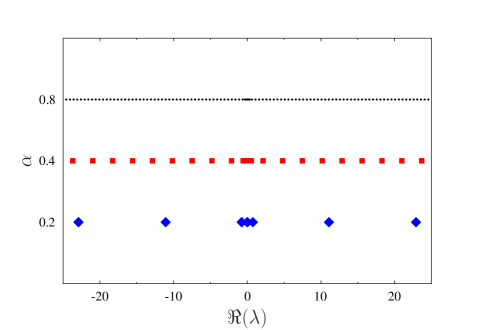
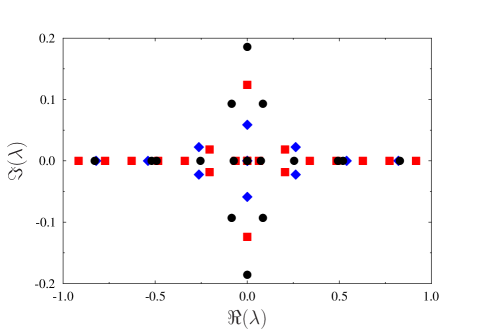
Figure 3: Spectra of eigenvalue problem (52) obtained for Norbury’s vortices with (a) $\alpha=0.2$ (blue diamonds), $\alpha=0.4$ (red squares), $\alpha=0.8$ (black circles) and (b) $\alpha=0.975$ (blue diamonds), $\alpha=1.2$ (red squares), $\alpha=1.39$ (black circles). In panel (a) all eigenvalues are purely real and, for clarity, the vertical axis is not scaled uniformly.

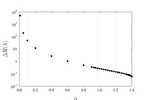
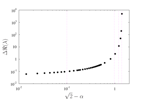
Figure 4: Dependence of the average difference $\Delta\Re(\lambda)$ between two consecutive purely real eigenvalues on (a) the parameter $\alpha$ with the linear scaling and (b) the quantity $(\sqrt{2}-\alpha)$ with the logarithmic scaling. The dotted vertical lines represent the values of $\alpha$ for which the unstable and certain neutrally stable eigenvectors are analyzed in figures 7, 8 and 9.

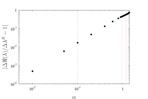
Figure 5: Dependence of the relative difference between the quantity $\Delta\Re(\lambda)$, cf. figure 4, and the quantity $\Delta\lambda^{R}$ characterizing the stability spectrum of Rankine’s vortex on the parameter $\alpha$. The dotted vertical lines represent the values of $\alpha$ for which the unstable and certain neutrally stable eigenvectors are analyzed in figures 7, 8 and 9.

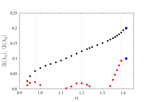
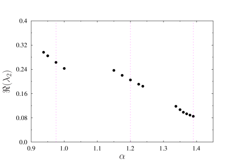
Figure 6: Dependence of (a) the imaginary parts of the unstable eigenvalues $\lambda_{1}$ (black circles) and $\lambda_{2}$ (red squares) and (b) the real part of the unstable eigenvalue $\lambda_{2}$ on the parameter $\alpha$. The blue diamonds in panel (a) represent the eigenvalues characterizing the stability of Hill’s vortex (Moffatt & Moore, 1978; Protas & Elcrat, 2016). Since due to the reasons discussed at the end of §4 the eigenvalue $\lambda_{2}$ could not be reliably determined when $\alpha=1.4$, it is not shown in these figures. The dotted vertical lines represent the values of $\alpha$ for which the unstable eigenvectors are analyzed in figures 7 and 8.

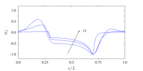
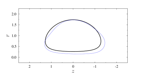
(a) $\alpha=0.975$

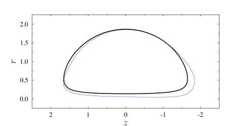
(b) $\alpha=1.2$

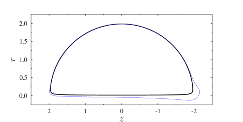
(c) $\alpha=1.39$

Figure 7: (a) Unstable purely real eigenvectors $u_{1}$ obtained for $\alpha=0.975,1.2,1.39$ presented as functions of the normalized arclength coordinate $s/L$ along the vortex boundary $\partial A$ (the arrow indicates the trend when $\alpha$ increases). (b–d) Deformations of the vortex boundary induced by the eigenvectors $u_{1}$ for the indicated values of $\alpha$ (the magnitude of the perturbation, given by $\epsilon$ in ansatz (18), is arbitrary). The thick lines represent the vortex boundaries $\partial{\mathcal{A}}$ in their equilibrium configurations. In this and in subsequent figures the eigenvectors are scaled such that $\max_{s\in[0,L]}|u(s)|=1$.

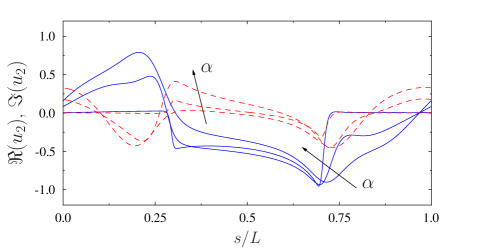
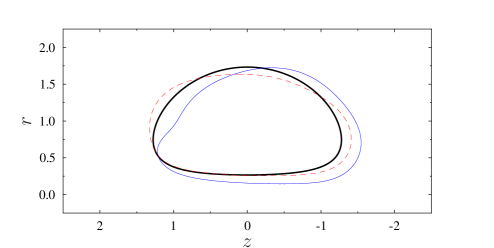
(a) $\alpha=0.975$

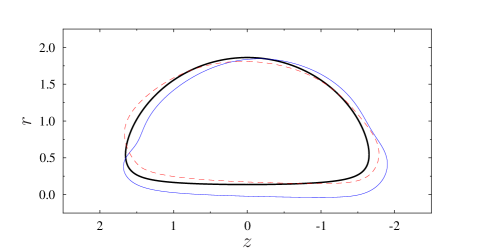
(b) $\alpha=1.2$

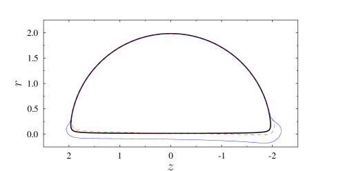
(c) $\alpha=1.39$

Figure 8: (a) Real parts (blue solid lines) and imaginary parts (red dashed lines) of the unstable eigenvectors $u_{2}$ obtained for $\alpha=0.975,1.2,1.39$ presented as functions of the normalized arclength coordinate $s/L$ along the vortex boundary $\partial A$ (the arrow indicates the trend when $\alpha$ increases). (b–d) Deformations of the vortex boundary induced by the real and imaginary parts of the eigenvectors $u_{2}$ for the indicated values of $\alpha$ (the magnitude of the perturbation, given by $\epsilon$ in ansatz (18), is arbitrary). The thick lines represent the vortex boundaries $\partial{\mathcal{A}}$ in their equilibrium configurations.

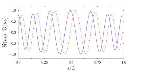
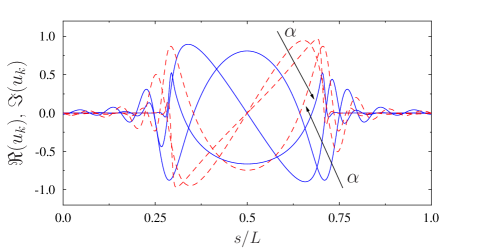
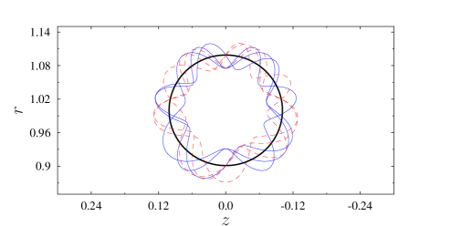
(a) $\alpha=0.1$

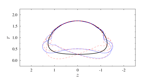
(b) $\alpha=0.975$

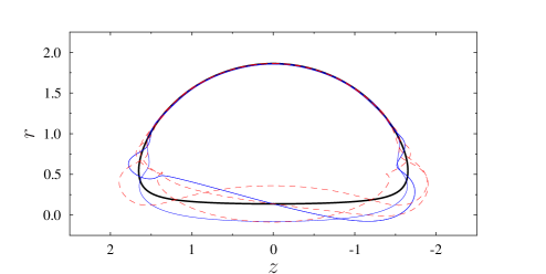
(c) $\alpha=1.2$

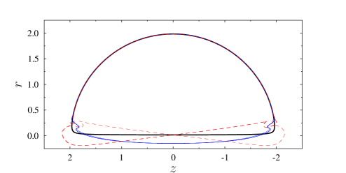
(d) $\alpha=1.39$

Figure 9: Real parts (blue solid lines) and imaginary parts (red dashed lines) of representative neutrally stable eigenvectors $u_{k}$ obtained for (a) $\alpha=0.1$ and (b) $\alpha=0.975,1.2,1.39$ presented as functions of the normalized arclength coordinate $s/L$ along the vortex boundary $\partial A$ (the arrows in panel (b) indicate the trends when $\alpha$ increases). The eigenvectors are associated with purely real eigenvalues $\lambda_{k}$ close to $\pm 0.05$. (c–f) Deformations of the vortex boundary induced by the real and imaginary parts of these neutrally stable eigenvectors for the indicated values of $\alpha$ (the magnitude of the perturbation, given by $\epsilon$ in ansatz (18), is arbitrary). The thick lines represent the vortex boundaries $\partial{\mathcal{A}}$ in their equilibrium configurations.

We now move on to discuss the eigenvectors of problem (28) focusing on how their structure depends on the parameter $\alpha$. We begin with the unstable eigenvectors corresponding to the eigenvalues $\lambda_{1}$ and $\lambda_{2}$, denoted $u_{1}$ and $u_{2}$, which we will consider for representative values of the parameter $\alpha$ chosen from each of the three subintervals of $\alpha$ where $\Im(\lambda_{2})\neq 0$, cf. figure 6(a). We remark that when ansatz (27) is used and the eigenvalue $\lambda$ turns out to be purely imaginary, then the imaginary part of the corresponding eigenvector $u$ is irrelevant for the stability analysis (in fact, in the present computations it vanishes identically in such cases). On the other hand, if the eigenvalue $\lambda$ is complex, then both the real and imaginary part of the eigenvector $u$ play a role in the stability analysis. We add that purely imaginary eigenvalues correspond to exponential in time growth of the normal perturbations $\rho(t,s)$ to the vortex boundary $\partial{\mathcal{A}}$, cf. ansätze (18) and (27), whereas for complex eigenvalues this exponential growth is combined with harmonic oscillations.

The unstable eigenvectors $u_{1}$ obtained for $\alpha=0.975,1.2,1.39$ are compared as functions of the normalized arclength coordinate $s/L$ measured counterclockwise along the vortex boundary $\partial A$ in figure 7(a) (the arclength coordinate is measured starting from the outer intersection of the vortex boundary $\partial A$ with the $r$-axis, cf. $\theta=0$ in figure 1, whereas $L:=\int_{\partial A}\,ds$ is the length of the vortex boundary). Deformations of the vortex boundary $\partial A$ induced by these eigenvectors are shown for the different values of $\alpha$ in figures 7(b–d). We note that for all considered values of $\alpha$ the deformation of the vortex boundary is concentrated near its rear (right) extremity and becomes more localized as $\alpha$ increases which is accompanied by the formation of a high-curvature region in the vortex boundary. We also observe that away from the rear extremity of the vortex the eigenvectors $u_{1}$ deform the boundary $\partial A$ in an opposite sense, which is a consequence of the constraint requiring the perturbations to preserve the circulation, cf. (23). The real and imaginary parts of the eigenvectors $u_{2}$ associated with the second eigenvalue $\lambda_{2}$ obtained for different values of $\alpha$ are shown in figure 8(a) as functions of the normalized arclength coordinate $s/L$, with the corresponding deformations of the vortex boundary $\partial A$ illustrated in figures 8(b–d). Here, for both the real and imaginary parts of the eigenvectors we observe properties qualitatively similar to what was already noted for the eigenvectors $u_{1}$ in figure 7 with the eigenvectors $u_{2}$ also becoming increasingly localized near the rear extremity of the vortex as $\alpha$ increases. We emphasize that this behavior is indeed consistent with the stability properties of Hill’s vortex, corresponding to $\alpha=\sqrt{2}$, where the unstable eigenvectors $u_{1}$ and $u_{2}$ were found to have the form of singular distributions localized at the rear stagnation point (Protas & Elcrat, 2016). The unstable eigenvectors $u_{2}$ also have the interesting property that while their real and imaginary parts deform the equilibrium contour in the same sense near the rear extremity of the vortex ring, they do so in an opposite sense near the front extremity. We add that since the eigenvalues with nonzero imaginary parts come in conjugate pairs, cf. figure 3(b), for each unstable mode there is a corresponding stable mode. These stable eigenvectors have the form $u_{1}(L-s)$ and $u_{2}(L-s)$ for $s\in[0,L]$, i.e., they are obtained from the unstable modes by reflecting them with respect to the symmetry axis of the vortex region $A$, such that they become localized near its front (left) extremity as $\alpha\rightarrow\sqrt{2}$.

Finally, we move on to discuss the dependence of the neutrally stable eigenvectors, denoted $u_{k}$, $k\neq 1,2$, associated with the purely real eigenvalues on the parameter $\alpha$. Extrapolating the data shown in figure 3(a), we note that for all values of $\alpha\in(0,\sqrt{2})$ there is a countable infinity of neutrally-stable eigenvectors, although only a finite subset of these eigenvectors may be resolved with computations performed with a finite resolution $M$. Thus, to fix attention, we will focus here on a few representative eigenvectors associated with eigenvalues $\lambda_{k}$ close to $\pm 0.05$. The real and imaginary parts of these eigenvectors obtained for Norbury’s vortices with $\alpha=0.1$ and $\alpha=0.975,1.2,1.39$ are shown as functions of the normalized arclength coordinate $s/L$ along the vortex boundary $\partial A$ in figures 9(a) and 9(b), respectively, whereas the deformations of the vortex boundaries induced by these eigenvectors are illustrated in figures 9(c–f). In figures 9(a) and 9(c) we see that for small values of $\alpha$, when the vortex region $A$ is nearly circular, cf. figure 2(a), the eigenvectors have the form of a nearly harmonic oscillation with a small modulation and with the real and imaginary parts differing only by a phase shift. In fact, in the thin-vortex limit $\alpha\rightarrow 0$ these eigenvectors approach Kelvin waves (i.e., purely harmonic oscillations) known to characterize the neutral stability of Rankine’s vortex (Lamb, 1932). On the other hand, for $\alpha\rightarrow\sqrt{2}$ the neutrally stable eigenvectors have the form of oscillations which are increasingly localized near the front (left) and rear (right) extremity of the vortex region, a behavior which in the limit is also consistent with the stability properties of Hill’s vortex (Protas & Elcrat, 2016). In general, for a given $\alpha$ the number of oscillations exhibited by the neutrally stable eigenvectors increases with $|\Re(\lambda_{k})|$.

6 Summary and Conclusions

In this final section we briefly summarize and discuss our results before pointing to some open questions. Recognizing that Norbury’s vortex rings are solutions to the free-boundary problem (1)–(2), their stability to axisymmetric perturbations was studied here using an approach based on the shape-differential calculus which allows one to rigorously account for the effect of perturbations to the shape of the vortex boundary in the linearization of the governing equations, cf. §3. In addition to axisymmetry, the perturbations are assumed not the change the circulation $\Gamma$ of the vortex ring from its equilibrium configuration. Such perturbations may be therefore regarded as resulting from the application of conservative forces to the vortex ring. Information about the stability of the vortex rings to such axisymmetric and circulation-preserving perturbations is then encoded in the spectrum of a singular integro-differential operator (24a) defined on the vortex boundary $\partial A$ in the meridional plane. After discretizing it with a spectrally-accurate numerical technique and imposing the constraint ensuring that perturbations preserve the circulation of the vortex ring, we obtain a constrained eigenvalue problem which is solved numerically. Developed and validated by Elcrat & Protas (2013), this approach was used earlier to solve an analogous stability problem for Hill’s vortex (Protas & Elcrat, 2016). The base states (Norbury’s vortex rings) were recomputed using Newton’s method based on shape-differentiation to ensure that they are determined with a much higher accuracy and for a broader range of the parameter $\alpha$ than in Norbury’s original work (Norbury, 1973). The data for these base states is provided as Supplementary Information accompanying this paper.

The results presented in §5 demonstrate that in terms of stability properties with respect to axisymmetric perturbations the continuous family of Norbury’s vortex rings represents a “bridge” connecting Rankine’s columnar vortex with Hill’s spherical vortex. Indeed, for small $\alpha\in(0,\alpha_{0}]$, Norbury’s vortex rings are neutrally stable with the eigenvectors and eigenvalues approaching Kelvin waves and their eigenvalues in the thin-vortex limit $\alpha\rightarrow 0$. The fact that the stability properties of Rankine’s vortex are recovered in this limit can be explained by the observation that in this case a thin vortex ring can be treated as an isolated columnar (Rankine) vortex and under the assumption of axisymmetry perturbations are allowed in the meridional plane only where they give rise to Kelvin waves. As $\alpha$ increases and the vortex rings grow fatter, they become unstable at $\alpha_{0}\approx 0.925$ which is marked by the emergence of two unstable eigenmodes. There seems to be no obvious change to the form of the vortex region ${\mathcal{A}}$ or to the corresponding flow pattern to which this change of stability could be attributed. However, as observed by O’Farrell & Dabiri (2012), the change of stability can be explained by the fact that as $\alpha$ increases parts of the vortex boundary approach the rear stagnation point (which is on the flow axis) such that the resulting shear becomes strong enough to amplify the perturbation. On the other hand, for thin vortex rings corresponding to small values of $\alpha$, the shear affecting the vortex boundaries is rather weak and perturbations are swept along the vortex perimeter without amplification. The most unstable mode $u_{1}$ is associated with a purely imaginary eigenvalue $\lambda_{1}$ whose imaginary part increases in magnitude monotonically with $\alpha$, cf. figure 6(a). Interestingly, the second unstable eigenmode $u_{2}$ is present only for certain values of the parameter $\alpha\in[\alpha_{0},\sqrt{2})$. It is associated with the eigenvalue $\lambda_{2}$ with a nonvanishing real part whose magnitude deceases with $\alpha$, cf. figure 6(b). As a result, in the fat-vortex limit $\alpha\rightarrow\sqrt{2}$ the two unstable eigenvalues $\lambda_{1}$ and $\lambda_{2}$ converge to the eigenvalues associated with the two unstable eigenvectors of Hill’s vortex, while the corresponding eigenvectors $u_{1}$ and $u_{2}$ become increasingly localized near the rear extremity of the vortex. In the limit $\alpha\rightarrow\sqrt{2}$ this high-curvature region becomes the rear stagnation point of Hill’s vortex. The two unstable eigenmodes of Hill’s vortex have the form of singular distributions localized at that point (Protas & Elcrat, 2016) and can be therefore regarded as the limits the unstable eigenvectors $u_{1}$ and $u_{2}$ of Norbury’s vortices converge to as $\alpha\rightarrow\sqrt{2}$, cf. figures 7(a) and 8(a). We add that analogous results concerning the stability of Hill’s vortex to axisymmetric circulation-preserving perturbations had been earlier obtained using different techniques by Moffatt & Moore (1978). At the same time, the set of purely real eigenvalues converges to the continuous spectrum which was also reported for Hill’s vortex, although the convergence is rather slow, cf. figure 4(b). Finally, we add that the properties of the stability spectra obtained here for Norbury’s vortex rings with different values of $\alpha$, cf. figures 3(a) and 3(b), are consistent with the Hamiltonian structure of the governing Euler equations, in the sense that in all cases the sum of the eigenvalues is zero.

The stability results summarized above are consistent with the responses of Norbury’s vortex rings to axisymmetric perturbations computed in the nonlinear regime by O’Farrell & Dabiri (2012), see also Ye & Chu (1995). More specifically, for thin vortex rings O’Farrell & Dabiri (2012) found that small perturbations to the vortex boundary travel around the vortex perimeter, which is consistent with the neutral stability reported in this regime in the present study. On the other hand, for fat vortex rings they observed that prolate perturbations of the shape of the vortex boundary are amplified and evolve into protrusions near the rear extremity of the vortex ring which then move upstream to become thin filaments. This behavior too is consistent with the results of our analysis which predicts that fat vortex rings are linearly unstable to axisymmetric perturbations and in fact the deformation of the vortex boundary near the rear extremity of the vortex ring characterizing the most unstable eigenmodes, cf. figure 7, can be viewed as a precursor of the filament observed at later stages of the evolution by O’Farrell & Dabiri (2012). Moreover, the value of the parameter $\alpha$ demarcating the two regimes reported by O’Farrell & Dabiri (2012) was $\alpha=0.7$, not too far from $\alpha_{0}=0.925$ found here.

We reiterate that the physical significance of the results reported here is clearly restricted by the assumption of axisymmetry introduced to simplify the problem, which limits the class of admissible perturbations. More specifically, while the present analysis indicates that thin vortex rings are neutrally stable, they are in fact known to be linearly unstable and develop a bending instability when subject to perturbations depending on the azimuthal coordinate (Fukumoto & Hattori, 2005, see Introduction for more discussion). In the same spirit, for Hill’s vortex the studies of Fukuyu et al. (1994); Rozi (1999) demonstrated that perturbations with dependence on the azimuthal angle $\phi$ which are still localized near the rear stagnation point have in fact larger growth rates than the unstable modes with axial symmetry discussed by Moffatt & Moore (1978); Protas & Elcrat (2016). Thus, the ultimate goal of this research program is to address this limitation and provide a complete understanding of the stability of inviscid vortex rings with respect to general perturbations; the present results are a stepping stone in this direction. This more general stability problem can be studied using methods analogous to the approach developed in §3, except that the perturbation $\rho$ will now also depend on the azimuthal angle $\phi$ and the standard form of the Biot-Savart kernel will need to be used in lieu of ${\bf K}$ in (18)–(19). Consequently, the eigenvalue problem corresponding to (28) will have both $\theta$ and $\phi$ as independent variables. Solving this problem will be our next step and results will be reported in the near future.

Appendix A Evaluation of Improper Integrals $C_{k}(\theta)$ and $S_{k}(\theta)$

In this appendix we derive expressions (40a) and (40b) for the improper integrals $C_{k}(\theta)$ and $S_{k}(\theta)$. Since these integrals can be evaluated using standard techniques when $k=0$, here we focus on the case when $k\geq 1$ and consider $C_{k}(\theta)$. The integral is first transformed using standard trigonometric identities as

$$C_{k}(\theta) =\int_{0}^{2\pi}\cos(k\theta^{\prime})\ln\sin^{2}\left(\frac{\theta-\theta^{\prime}}{2}\right)\,d\theta^{\prime}$$

$$=\frac{1}{2}\int_{0}^{2\pi}e^{ik\theta^{\prime}}\ln\left[\frac{e^{\frac{i(\theta-\theta^{\prime})}{2}}-e^{-\frac{i(\theta-\theta^{\prime})}{2}}}{2i}\right]^{2}\,d\theta^{\prime}+\frac{1}{2}\int_{0}^{2\pi}e^{-ik\theta^{\prime}}\ln\left[\frac{e^{\frac{i(\theta-\theta^{\prime})}{2}}-e^{-\frac{i(\theta-\theta^{\prime})}{2}}}{2i}\right]^{2}\,d\theta^{\prime}$$

$$=:{\xi}_{k}(\theta)+\chi_{k}(\theta).$$ (53)

Since evidently $\chi_{k}(\theta)=\overline{{\xi}}_{k}(\theta)$, where the overbar denotes complex conjugation, below we need to consider only ${\xi}_{k}(\theta)$. This integral is mapped to the unit circle $C:=\left\{w\in{\mathbb{C}},\ |w|=1\right\}$ in the complex plane using the substitutions $w=e^{\i\theta}$ and $-idw=e^{i\theta}\,d\theta$

$${\xi}_{k}(\theta)=-\frac{i}{2}\oint_{C}w^{\prime(k-1)}\ln\left[-\frac{(w-w^{\prime})^{2}}{4ww^{\prime}}\right]\,dw^{\prime}$$

$$=\frac{i}{2k}\oint_{C}\frac{w^{\prime k}+w^{\prime(k-1)}w}{w^{\prime}-w}\,dw^{\prime}=-\frac{\pi w^{k}}{k},$$ (54)

where the second equality follows from the integration by parts (since $w,w^{\prime}\in C$, the branch cut in the complex logarithm does not intersect the unit circle so that this operation is allowed), whereas the final result is obtained by applying Plemelj’s identity to the Cauchy-type singular integral (Muskhelishvili, 2008). Finally, using (53) and returning to the original variable $\theta$, we arrive at

$$C_{k}(\theta)={\xi}_{k}(\theta)+\overline{{\xi}}_{k}(\theta)=-\frac{\pi w^{k}}{k}-\frac{\pi\overline{w}^{k}}{k}=-\frac{2\pi}{k}\cos(k\theta).$$ (55)

Identity (40b) for $S_{k}(\theta)$ is determined following analogous steps.

References

- Akhmetov (2009) Akhmetov, D. G. 2009 Vortex Rings. Berlin, Heidelberg: Springer-Verlag.
- Alekseenko et al. (2007) Alekseenko, S.V., Kuibin, P.A. & Okulov, V.L. 2007 Theory of Concentrated Vortices: An Introduction. Springer Berlin Heidelberg.
- Arvidsson et al. (2016) Arvidsson, Per M., Kovács, Sándor J., Töger, Johannes, Borgquist, Rasmus, Heiberg, Einar, Carlsson, Marcus & Arheden, Håkan 2016 Vortex ring behavior provides the epigenetic blueprint for the human heart. Scientific Reports 6, 22021 EP –, article.
- Baker (1990) Baker, G. R. 1990 A study of the numerical stability of the method of contour dynamics. Phil. Trans. Roy. Soc. 333, 391–400.
- Berezovskii & Kaplanskii (1992) Berezovskii, A.A. & Kaplanskii, F.B 1992 Dynamics of thin vortex rings in a low-viscosity fluid. Fluid Dynamics 27, 643–649.
- Boyd (2001) Boyd, J. P. 2001 Chebyshev and Fourier Spectral Methods. Dover.
- Brooke Benjamin (1975) Brooke Benjamin, T. 1975 The alliance of practical and analytical insights into the nonlinear problems of fluid mechanics. In Proc. Symp. on Applications of Methods of Functional Analysis to Problems in Mechanics, , vol. 503. Springer.
- Dabiri (2009) Dabiri, J. O. 2009 Optimal vortex formation as a unifying principle in biological propulsion. Annual Review of Fluid Mechanics 41 (1), 17–33.
- Delfour & Zolésio (2001) Delfour, M. C. & Zolésio, J.-P. 2001 Shape and Geometries — Analysis, Differential Calculus and Optimization. SIAM.
- Dritschel (1985) Dritschel, D. G. 1985 The stability and energetics of corotating uniform vortices. J. Fluid Mech. 157, 95–134.
- Dritschel (1990) Dritschel, D. G. 1990 The stability of elliptical vortices in an external straining flow. J. Fluid Mech. 210, 223–261.
- Dritschel (1995) Dritschel, D. G. 1995 A general theory for two–dimensional vortex interactions. J. Fluid Mech. 293, 269–303.
- Dritschel & Legras (1991) Dritschel, D. G. & Legras, B. 1991 The elliptical models of two-dimensional vortex dynamics. II: Disturbance equations. Phys. Fluids A 3, 855–869.
- Elcrat et al. (2005) Elcrat, A., Fornberg, B. & Miller, K. 2005 Stability of vortices in equilibrium with a cylinder. J. Fluid Mech. 544, 53–68.
- Elcrat & Protas (2013) Elcrat, A. & Protas, B. 2013 A framework for linear stability analysis of finite-area vortices. Proceedings of the Royal Society A 469, 20120709.
- Fraenkel (1970) Fraenkel, L. E. 1970 On steady vortex rings of small cross-section in an ideal fluid. Proceedings of the Royal Society of London A: Mathematical, Physical and Engineering Sciences 316 (1524), 29–62.
- Fukumoto & Hattori (2005) Fukumoto, Yasuhide & Hattori, Yuji 2005 Curvature instability of a vortex ring. Journal of Fluid Mechanics 526, 77–115.
- Fukumoto & Kaplanski (2008) Fukumoto, Y. & Kaplanski, F. B. 2008 Global time evolution of an axisymmetric vortex ring at low reynolds numbers. Phys. Fluids 20, 053103.
- Fukumoto & Moffatt (2000) Fukumoto, Y. & Moffatt, H. K. 2000 Motion and expansion of a viscous vortex ring. part 1. a higher-order asymptotic formula for the velocity. J. Fluid Mech. 417, 1–45.
- Fukumoto & Moffatt (2008) Fukumoto, Y. & Moffatt, H. K. 2008 Kinematic variational principle for motion of vortex rings. Physica D 237, 2210–2217.
- Fukuyu et al. (1994) Fukuyu, A., Ruzi, T. & Kanai, A. 1994 The response of Hill’s vortex to a small three dimensional disturbance. J. Phys. Soc. Japan 63, 510–527.
- Gallay & Smets (2018) Gallay, Th. & Smets, D. 2018 Spectral stability of inviscid columnar vortices. ArXiv:1805.05064.
- Giannuzzi et al. (2016) Giannuzzi, P. M., Hargather, M. J. & Doig, G. C. 2016 Explosive-driven shock wave and vortex ring interaction with a propane flame. Shock Waves 26 (6), 851–857.
- Golub (1973) Golub, G. 1973 Some modified matrix eigenvalue problems. SIAM Review 15 (2), 318–334.
- Graber (2015) Graber, Curtis E. 2015 Vortex cannon with enhanced ring vortex generation. US Patent US9217392B2.
- Gumowski et al. (2008) Gumowski, K., Miedzik, J., Goujon-Durand, S., Jenffer, P. & Wesfreid, J. E. 2008 Transition to a time-dependent state of fluid flow in the wake of a sphere. Phys. Rev. E 77, 055308.
- Guo et al. (2004) Guo, Y., Hallstrom, Ch. & Spirn, D. 2004 Dynamics Near an Unstable Kirchhoff Ellipse. Commun. Math. Phys. 245, 297–354.
- Hackbusch (1995) Hackbusch, W. 1995 Integral Equations: Theory and Numerical Treatment. Birkhäuser.
- Hattori & Fukumoto (2003) Hattori, Y. & Fukumoto, Y. 2003 Short-wavelength stability analysis of thin vortex rings. Physics of Fluids 15 (10), 3151–3163.
- Hattori & Hijiya (2010) Hattori, Y. & Hijiya, K. 2010 Short-wavelength stability analysis of Hill’s vortex with/without swirl. Phys Fluids 22, 074104.
- Hicks (1899) Hicks, W. M. 1899 Ii. researches in vortex motion. —part iii. on spiral or gyrostatic vortex aggregates. Philosophical Transactions of the Royal Society of London A: Mathematical, Physical and Engineering Sciences 192, 33–99.
- Hill (1894) Hill, M. J. M. 1894 On a spherical vortex. Philos. Trans. Roy. Soc. London A185, 213–245.
- Kamm (1987) Kamm, J. R. 1987 Shape and stability of two–dimensional vortex regions. PhD thesis, Caltech.
- Kaplanski & Rudi (2005) Kaplanski, F. B. & Rudi, Y. A. 2005 A model for the formation of "optimal" vortex ring taking into account viscosity. Phys. Fluids 17, 087101–087107.
- Kelvin (1867) Kelvin, Lord 1867 The traslatory velocity of a circular vortex ring. Phil. Mag. 33, 511––512.
- Kelvin (1880) Kelvin, Lord 1880 Vibrations of a columnar vortex. Phil. Mag. 10, 155–168.
- Kheradvar & Pedrizzetti (2012) Kheradvar, A. & Pedrizzetti, G. 2012 Vortex Formation in the Cardiovascular System. Springer.
- Lamb (1932) Lamb, H. 1932 Hydrodynamics. Dover, New York.
- Laub (2005) Laub, A. J. 2005 Matrix Analysis for Scientists and Engineers. SIAM.
- Lifschitz (1995) Lifschitz, A. 1995 nstabilities of ideal fluids and related topics. Z. Angew. Math. Mech. 75, 411.
- Lifschitz & Hameiri (1991) Lifschitz, A. & Hameiri, E. 1991 Local stability conditions in fluid dynamics. Phys. Fluids A 3, 2644–2651.
- Llewellyn Smith & Ford (2001) Llewellyn Smith, S. G. & Ford, R. 2001 Three-dimensional acoustic scattering by vortical flows. Part I: General theory. Phys. Fluids 13, 2876–2889.
- Love (1893) Love, A. E. H. 1893 On the stability of certain vortex motions. Proc. London Math. Soc. s1–25, 18–43.
- Maxworthy (1977) Maxworthy, T. 1977 Some experimental studies of vortex rings. Journal of Fluid Mechanics 81 (3), 465–495.
- Moffatt & Moore (1978) Moffatt, H. K. & Moore, D. W. 1978 The response of Hill’s spherical vortex to a small axisymmetric disturbance. J. Fluid Mech. 87, 749–760.
- Mohseni (2001) Mohseni, K. 2001 Statistical equilibrium theory for axisymmetric flow: Kelvin’s variationalprinciple and an explanation for the vortex ring pinch–off process. Phys. Fluids 13, 1924.
- Moore & Saffman (1975) Moore, D. W. & Saffman, P. G. 1975 The instability of a straight vortex filament in a strain field. Proceedings of the Royal Society of London A: Mathematical, Physical and Engineering Sciences 346 (1646), 413–425.
- Muskhelishvili (2008) Muskhelishvili, N. I. 2008 Singular Integral Equations. Boundary Problems of Function Theory and Their Application to Mathematical Physics, 2nd edn. Dover.
- Norbury (1972) Norbury, J. 1972 A steady vortex ring close to Hill’s spherical vortex. Proc. Cambridge Phil. Soc. 72, 253–282.
- Norbury (1973) Norbury, J. 1973 A family of steady vortex rings. J. Fluid Mech. 57, 417–431.
- O’Farrell & Dabiri (2012) O’Farrell, Clara & Dabiri, John O. 2012 Perturbation response and pinch-off of vortex rings and dipoles. Journal of Fluid Mechanics 704, 280–300.
- Olver et al. (2010) Olver, F. W. J., Lozier, D. W., Boisvert, R. F. & Clark, C. W., ed. 2010 NIST Handbook of Mathematical Functions. New York, NY: Cambridge University Press.
- Pozrikidis (1986) Pozrikidis, C. 1986 The nonlinear instability of Hill’s vortex. J. Fluid Mech. 168, 337 – 367.
- Protas & Elcrat (2016) Protas, Bartosz & Elcrat, Alan 2016 Linear stability of Hill’s vortex to axisymmetric perturbations. Journal of Fluid Mechanics 799, 579–602.
- Pullin (1992) Pullin, D. I. 1992 Contour dynamics methods. Annual Review of Fluid Mechanics 24, 89–115.
- Rozi (1999) Rozi, T. 1999 Evolution of the Surface of Hill’s Vortex Subjected to a Small Three-Dimensional Disturbance for the Cases of and 4. J. Phys. Soc. Japan 68, 2940.
- Rozi & Fukumoto (2000) Rozi, T. & Fukumoto, Y. 2000 The Most Unstable Perturbation of Wave-Packet Form Inside Hill’s Vortex. J. Phys. Soc. Japan 69, 2700–2701.
- Saffman (1970) Saffman, P. G. 1970 The velocity of viscous vortex rings. Studies in Applied Math. 49, 371.
- Saffman (1992) Saffman, P. G. 1992 Vortex Dynamics. Cambridge, New York: Cambridge University Press.
- Shariff et al. (2008) Shariff, K., Leonard, A. & Ferziger, J. H. 2008 A contour dynamics algorithm for axisymmetric flow. Journal of Computational Physics 227, 9044–9062.
- Trefethen (2000) Trefethen, L. N. 2000 Spectral Methods in Matlab. SIAM.
- Trefethen (2013) Trefethen, N. 2013 Approximation Theory and Approximation Practice. SIAM.
- Tung & Ting (1967) Tung, C. & Ting, L. 1967 Motion and decay of a vortex ring. Phys. Fluids 10, 901–910.
- Wakelin & Riley (1996) Wakelin, S. L. & Riley, N. 1996 Vortex ring interactions ii. inviscid models. Quarterly Journal of Mechanics and Applied Mathematics 49, 287–309.
- Wan (1988) Wan, Y. H. 1988 Variational principles for Hill’s spherical vortex and nearly spherical vortices. Trans. Amer. Math. Soc. 308, 299–312.
- Widnall et al. (1974) Widnall, Sheila E., Bliss, Donald B. & Tsai, Chon-Yin 1974 The instability of short waves on a vortex ring. Journal of Fluid Mechanics 66 (1), 35–47.
- Widnall et al. (1973) Widnall, Sheila. E., Sullivan, J. P. & Owen, Paul Robert 1973 On the stability of vortex rings. Proceedings of the Royal Society of London. A. Mathematical and Physical Sciences 332 (1590), 335–353.
- Widnall et al. (1977) Widnall, Sheila. E., yin Tsai, Chon & Stuart, John Trevor 1977 The instability of the thin vortex ring of constant vorticity. Philosophical Transactions of the Royal Society of London. Series A, Mathematical and Physical Sciences 287 (1344), 273–305.
- Wu et al. (2006) Wu, J.-Z., Ma, H.-Y. & Zhou, M.-D. 2006 Vorticity and vortex dynamics. Berlin, Heidelberg, New York: Springer-Verlag.
- Ye & Chu (1995) Ye, Qu-Yuan & Chu, C. K. 1995 Unsteady evolutions of vortex rings. Physics of Fluids 7 (4), 795–801.