An introduction to Bootstrap for nuclear physics

Abstract

This guide aims at providing a general introduction to bootstrap methods. By using simple examples taken from nuclear physics, I discuss how such a method can be used to quantify error bars of an estimator. I also investigate the use of bootstrap to estimate parameters of a simple liquid drop model. In particular, I investigate how the method compares with standard techniques based on likelihood estimator and how to take into account correlations to better evaluate confidence interval of parameters.

I Introduction

In statistics, an estimator is a rule that applied to the sample data returns information on the underlying population. Common estimators are the mean and the variance.

Following Ref. R.J.Barlow (1989), a good estimator should obey three criteria: consistency, efficiency and being unbiased.

• Consistent: in the limit of a sample size approching the whole population, the estimator get closer and closer to the true value.

• Efficient: the variance of the estimator, i.e. the fluctuations around the true value, should be small.

• Unbiased: for any sample size N, the estimator should on average always produce an answer close to the true value.

For example, I can define the following estimators to determine the average height of a given population provided a sample of size $N$

• $\hat{a}_{1}$: add up all the heigths and divide by N.

• $\hat{a}_{2}$: select one random observable. Ignore the rest.

• $\hat{a}_{3}$:add up all the heigths and divide by N-1.

One notices that only estimator $\hat{a}_{1}$ from the previous list respects all the three criteria at once. $\hat{a}_{2}$ is not consistent, while $\hat{a}_{3}$ is biased.

A common method used to define an estimator is the Maximum Likelihood Estimator (MLE). The MLE finds the set of parameters one wants to estimate that maximise the likelihood function given that specific data-set. The estimator built from MLE is usually efficient and consistent, but in most cases biased R.J.Barlow (1989). As a consequence it is important to evaluate the bias and thus use it to correct predictions.

An essential ingredient for the MLE construction is to assume an underlying distribution for the data of the sample. In most cases a Gaussian assumption is reasonable, but not necessary always the most appropriate. For example, in the case of a rare radioactive decay, a Poisson distribution would be more suitable in describing data than a Gaussian. A well-known estimator built from a Gaussian MLE is the least-square (LS) estimator. LS is widely used to determine the parameters of a given model using informations extracted from data. In Ref. Dobaczewski et al. (2014), the authors have illustrated in much detail all the main features of the MLE and how to use it to derive errors. The latter are obtained by performing a second derivative of the likelihood function with respect to a given parameter. Although the procedure looks quite simple, in reality there are some important numerical issues in how performing numerical derivatives at good level of accuracy and at reasonable computational cost Roca-Maza et al. (2015).

In this guide, I will discuss bootsrap method as a statistical tool to evaluate the bias and confidence intervals of statistical estimators R.J.Barlow (1989) without the explicit use of a likelihood function. Efron in 1979 Efron (1979) introduced the basic idea behind bootstrap: given a data-set and a particular estimator; one builds new series of data-sets by resampling the original one. This defines a bootstrap sample. By applying the estimator at each of these bootstrap samples, one obtains its empirical distribution. The main hypothesis is that such a distribution is very close to the true one, so one can use it to obtain informations about the bias and the errors of the estimator. I refer to the vast available literature on the subject Efron (1979); Efron and Tibshirani (1994); Davison and Hinkley (1997); Chernick et al. (2011); Manly (2006); Chernick (2008) to demonstrate the validity of such a statement, . The procedure I described is usually referred to as Non-Parametric Bootstrap (NPB), to differentiate it from the case where some prior knowledge on the underlying distribution of a given estimator is given. One defines in this case a Parametric-Bootstrap (PB): the new data-sets are randomly extracted from the postulated distribution as done in Ref. Pérez et al. (2014) and not from the original data-set.

Bootstrap has been rarely used in theoretical nuclear physics Nieves (2000); Pérez et al. (2014); Bertsch and Bingham (2017); Muir et al. (2018); Pasquini et al. (2018), despite its simplicity and high potential.The aim of the present guide is to introduce the basic formalism and apply it to simple models in nuclear physics.

The guide is organised as follow: in Sec.II, I introduce the basic idea behind bootstrap and I use it to evaluate confidence intervals of the mean and of the Pearson coefficients in two different scenario. In Sec.III, I discuss NPB application to parameter estimates of a simple Liquid Drop model with and without explicit correlations in the data-set. I present my conclusions in Sec.IV.

II Bootstrap: basic concepts

NPB is based on the simple assumption that any experimental data-set contains informations on its parent distribution. As a consequence, if the data-set is sufficiently large, it is possible to replace the original parent distribution via the empirical one obtained via Monte Carlo methods Efron (1979).

In a more precise way, let’s assume I have a data-set formed by $n$ independent vectors $X=\left(x_{1},x_{2},\dots,x_{n}\right)$ and a real-valued estimator of the parameter $\hat{\theta}$. The origin of the data is not specified and thus they may be the result of a real experiment or of a simulation. I now resample them to create a series of new data-sets named $X^{*}$ and I apply the estimator $\hat{\theta}^{*}$. For the sake of simplicity I consider $n=5$. A possible outcome may look as

$$X^{*}_{1} = \left(x_{1},x_{1},x_{5},x_{2},x_{3}\right)\;,$$

$$X^{*}_{2} = \left(x_{2},x_{1},x_{5},x_{1},x_{4}\right)\;,$$

$$X^{*}_{3} = \left(x_{1},x_{3},x_{4},x_{3},x_{5}\right)\;,$$

$$X^{*}_{4} = \left(x_{2},x_{2},x_{2},x_{2},x_{5}\right)\;.$$

Notice that the resampling allows for repetitions. By applying the estimator at each one of the four bootstrap samples, $N_{\text{boot}}=4$, I obtain the experimental distribution. From the resulting histogram, I extract confidence intervals of $\hat{\theta}$ by defining the 68%quantile . The resampling assumes that the observables $x_{i}$ are independent. Applying NPB to correlated data destroys correlations and may lead to wrong conclusions. I will discuss in Sec.III.2 an extension of the technique to take into account the case of strongly correlated data-sets.

Concerning the size of the original sample, there is a strong debate in the literature and I refer the reader to Ref. Chernick (2008) for more details.The role of the size of the sample can be understood by considering the number of possible combinations one can build out of a given sample

$$\left(\begin{array}[]{c}2n-1\\ n\end{array}\right)=\frac{(2n-1)!}{n!(n-1)!}\;,$$ (3)

for a small sample of $n=10$, the number of possible bootstrap combinations is 92378. For $n=50$ the number of combinations grows to $\approx 10^{30}$. This number need to be as big as possible so that one can consider negligible the probability of drawing two times exactly the same sample and thus make sure all possible combinations can be extracted with equal probability. As a rule of thumb one needs at least a sample of size $~{}50$, but several authors consider safe using NPB applied to sample sizes of $\approx 10-20$ Fisher and Hall (1990); Chernick et al. (2011). In the following, I will make use of estimator that are not sensitive to the particular order of the observables in the data-set, as for example the mean. For such a reason I used Eq.3 to estimate the number of possible combinations. In the case of an estimator for which order matters, than one the number of possible sets is $n^{n}$.

The number of bootstrap samples should also be large to avoid introducing undesired bias. Using central limit theorem (for large samples), I assume that the difference between the empirical and real distribution follows a Gaussian distribution and the variance decreases as $\approx 1/N_{\text{boot}}$, where $N_{\text{boot}}$ is the number of bootstrap samplings. In the present article, due to the low computational cost of Monte-Carlo sampling, I will use typically $N_{\text{boot}}\approx 10^{4}$ and thus neglect the bias.

Before moving forward, it is important mentioning a tecnique very similar to NPB and named jackknife Miller (1974). In this case instead of resampling the full data-set one leaves out $m$ observables at the time and then one uses the remaining $N-m$ data to evaluate the estimator. Although it looks very similar to NPB, the mathematical hypothesis behind it are very different Tukey (1958). Jackknife is computationally less expensive than NPB, but it is specialised to obtain the variance of the estimator, while NPB gives access to the complete empirical distribution.

II.1 Example: confidence interval of the mean

I illustrate the power of bootstrap by applying it to the well-known case of the estimator of the mean $\hat{\mu}$ of a data-set $\{X_{1},X_{2},\dots,X_{N}\}$ of length $N$. In this example, I will consider a sample of size $N=10$ extracted from an exponential distribution with mean $\frac{1}{\lambda}=\frac{1}{2}$. In Tab.1, I report the values used for this example.

value	0.068	1.649	0.058	0.165	0.522	0.040	1.078	0.512	0.354	0.449
position	1	2	3	4	5	6	7	8	9	10

Table 1: Random values extracted from exponential distribution with mean $\frac{1}{\lambda}=\frac{1}{2}$.

To calculate the mean of the parent distribution, I use the estimator

$$\hat{\mu}=\frac{1}{N}\sum_{i=1}^{N}X_{i}\;.$$ (4)

In this particular case I obtain $\hat{\mu}=0.489$. The estimator is efficient, consistent and unbiased R.J.Barlow (1989), moreover for this particular case (knowing the distribution of the estimator) it is possible to calculate the resulting error bars using the formula

$$\sigma_{M}=\frac{\sigma}{\sqrt{N}}\;,$$ (5)

where $\sigma$ is the root mean square of the data-set. I obtain $\sigma_{M}=0.154$.

I now repeat the same analysis using NPB. In this case I perform a random sampling ($N_{boot}=10^{4}$) and I apply the estimator $\mu^{*}$. I group the results using an histogram as illustrated in Fig.1. On this figure, I also show the confidence interval of the NPB estimates by considering the lower (upper) quantiles defining 68% of the total counts.

The average value of the different means calculated via NPB is $\bar{\mu^{*}}=0.489_{-0.146}^{0.159}$. As expected the values coincide since, it is known that the estimator in Eq.4 has no bias. The error bars are not symmetric (since I assume no prior Gaussian distribution), but they are extremely close to the estimated value, thus showing that NPB is a reliable method.

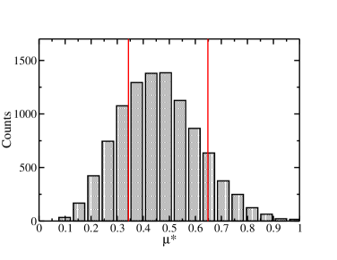
Figure 1: (Colors online) Confidence interval of the mean: distribution of occurrences of the value $\mu^{*}$ for the mean, Eq. 4, obtained from various NPB samples. The vertical lines indicate the confidence interval defining 68% of the total counts.

II.2 Example: confidence interval on Pearson coefficient

In this section, I consider another estimator, i.e. the Pearson coefficient R.J.Barlow (1989). The standard formulas to estimate errors of the Pearson coefficient are based on the Fisher transformation Corey et al. (1998). The latter is valid under the assumption of normally distributed data, so in case of outliers it is possible to obtain inconsistent results.

As an example, I consider the possible correlation between the slope of the symmetry energy $L_{0}$ and the neutron skin thickness $\Delta r_{np}$ of heavy nuclei Centelles et al. (2009); Roca-Maza et al. (2011).

In Fig.2, I show the neutron skin thickness in ²⁰⁸Pb as a function of $L_{0}$ extracted from several nuclear models. The data-set is composed by 63 nuclear functionals grouped in 3 big families: zero-range Skyrme functionals Perlińska et al. (2004); finite-range Gogny Dechargé and Gogny (1980) and Relativistic Lagrangians Bender et al. (2003); Nikšić et al. (2008) . For completeness, I report the models used in the calculation in Tab.5 with all relevant infinite nuclear matter properties.

The neutron skin thickness is extracted from the full quantal calculation using two point Fermi function (2pF) as detailed in Ref. Warda et al. (2010). The two horizontal lines represent the region compatible with the most recent experimental measurement of neutron skin thickness in ²⁰⁸Pb Tarbert et al. (2014) with its corresponding experimental error bars. To study the possible correlation between $L_{0}$ and $\Delta r_{np}$, I calculate the Pearson coefficient as

$$\hat{r}=\frac{\sum_{i=1}^{N}(X_{i}-\bar{X})(Y_{i}-\bar{Y})}{\sigma_{X}\sigma_{Y}}$$ (6)

where $\bar{X},\bar{Y}$ represent the mean values and $\sigma_{X,Y}$ the root mean square of the sample.

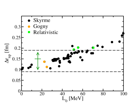
Figure 2: (Colors online) Neutron skin thickness in ²⁰⁸Pb as a function of $L_{0}$ for various nuclear models. The horizontal dashed line represent the experimental confidence interval as taken from Ref. Tarbert et al. (2014). See text for details.

For the present case I obtain $\hat{r}=0.91^{0.03}_{-0.05}$ where the error bars represent 95% confidence interval obtained using Fisher transformation. Performing NPB on the same data, I obtain a distribution of Pearson coefficient $r^{*}$ as shown in Fig.3. The vertical lines represent the region including the 95% counts.

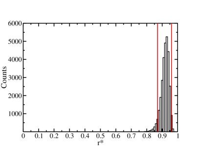
Figure 3: (Colors online) Confidence interval of the Pearson coefficient: distribution of occurrences of the values of $r^{*}$, Eq.6, obtained using various bootstrap data sets in ²⁰⁸Pb. The vertical lines represent the region including 95% of the counts.

The average value of the correlation coefficient extracted from NPB is

$$\bar{r}^{*}=0.92^{0.04}_{-0.04}\;.$$ (7)

The results are in excellent agreement between the two methods and with Refs Centelles et al. (2009); Roca-Maza et al. (2011). I conclude that the correlation in this data-set is very robust and very little dependent on the particular choice of the data used. This can be understood by looking at the distribution in Fig.3 and keeping in mind that not all data are used in every bootstrap resampling.

I repeat the previous analysis, but considering a different data-set to evaluate the impact of possible outliers when extracting statistical informations.

In Fig.4, I show the neutron skin thickness of ²⁰⁸Pb calculated with the same data-set reported in Tab.5, with an addition of extra 5 points (triangles). These points correspond to 5 Skyrme functionals with very large values of $L_{0}$: SEFM68 Dutra et al. (2012), SGOII  Shen et al. (2009), SKI1-2-5 Reinhard and Flocard (1995). These functionals produce a value of $L_{0}$ which is way too large compared to the acceptable values of $L_{0}$ Dutra et al. (2012). In this guide, I assume for simplicity that each observables can be resambles with the same probability. Given the prior knowledge on the acceptable values of $L_{0}$ Dutra et al. (2012), one may use instead the Bayesian version of bootstrap. I refer the reader to Refs. Rubin (1981); Boos and Monahan (1986) for more details on the method.

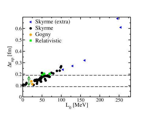
Figure 4: (Colors online) Same as Fig.2, but with 5 additional Skyrme functional (triangles).

I performed the same NPB analysis as before in ²⁰⁸Pb, but for this extended data-set. I obtain from NPB the value $\bar{r}^{*}=0.96^{0.03}_{-0.03}$. The distribution of $r^{*}$ reseambles very much the one reported in Fig.3, although much more narrow. The extra points do not change the conclusion of the previous section.

II.3 Example: confidence interval on Pearson coefficient with outliers

I now consider a different close shell nucleus: ¹⁰⁰Sn. In a previous study Muir et al. (2018), the authors have shown that there is no real correlation within $\Delta r_{np}$ and $L_{0}$ in the case of a close shell nucleus with equal number of neutrons and protons, since the possible presence of a proton skin is mainly driven by Coulomb interaction more than by symmetry energy properties.

This case is quite suitable to illustrate how the presence of outliers may lead to wrong conclusions when using the Pearson coefficient and the Fisher transformation to estimate error bars. In Fig.5, I show the neutron skin thickness of ¹⁰⁰Sn calculated with the same data-set reported in Tab.5, with an addition of extra 5 points (triangles). I use the same data set used to produce Fig.4.

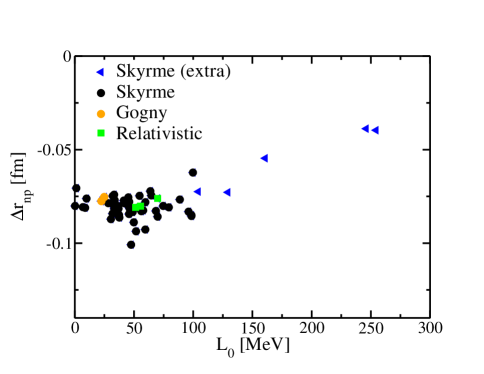
Figure 5: (Colors online) Neutron skin thickness in ¹⁰⁰Sn as a function of $L_{0}$ for various models. See text for details.

The Pearson coefficient calculated with these extra 5 Skyrme functionals leads to $\hat{r}=0.68^{0.11}_{-0.15}$. The correlation coefficient is smaller than the one obtained in ²⁰⁸Pb, but I can exclude with statistical significance the null-hypothesis of a non-correlated set.

In this case NPB may be very useful due to its random resampling nature: if the data are contaminated by few outliers, during random sampling most likely one will produce new data-sets with no outliers and thus getting strong variation on the estimator. Similar results would also be obtained using a much simpler jackknife method as illustrated in Ref. Efron (1979); Efron and Stein (1981). Actually this is a quite common procedure used to validate how the conclusions of a statistical analysis depend on the particular choice of the data sample.

In Fig.6, I report the empirical distribution of the Pearson estimators $r^{*}$ calculated using $N_{boot}=3\times 10^{4}$ Monte-Carlo samplings. Contrary to Fig.3, the distribution appears to be much more broad. The calculated mean value with 95% confidence error bar is $\bar{r}^{*}=0.58^{0.25}_{-0.59}$. Although the mean value of the estimator obtained with bootstrap is in good agreement with the direct calculation of the Pearson coefficient on the original the data-set, I observe that the error bars are much larger. As a consequence it is not possible to exclude the null-hypothesis of non-correlated data with a good statistical significance.

In this example, NPB is not used to identify which point is an outlier, but inspecting Fig.6, I can clearly observe a very large variance in the resulting estimator depending on the very specific choice of the observables of the data-set. This outcome should be used as a signal for a further investigation of the observables contained in the data-set.

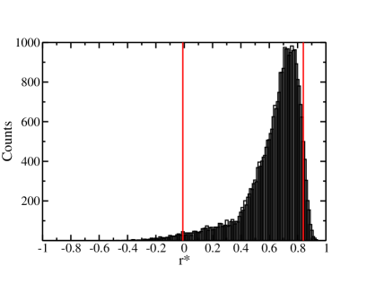
Figure 6: (Colors online) Confidence interval of the Pearson coefficient: distribution of occurrences of the values of $r^{*}$, Eq.6, obtained using various bootstrap data sets in ¹⁰⁰Sn. The vertical lines represent the region including 95% of the counts.

In this specific case, I decided to exclude the extra 5 points as done in Ref. Muir et al. (2018), by advokating the criteria on $L_{0}$ given in Ref Dutra et al. (2012). I obtain a result with a much more narrow distribution and centred on $r^{*}=0\pm 0.3$. It is important to stress the crucial role of error bars in this example. In both cases (with and without the 5 extra points) although the mean Pearson coefficient is very different, the error bars obtained via NPB lead always to the same conclusion: one can not exclude the null-hypothesis of non-correlated data.

III Regression analysis

Most of the models currently applied in theoretical nuclear physics rely on some adjustable parameters, usually obtained via LS minimisation Dobaczewski et al. (2014). In more general terms, the model function $M(\mathbf{x},\mathbf{p})$ depends on some input variables $\mathbf{x}$ and parameters $\mathbf{p}$. This function is derived under some assumptions and it contains our knowledge of a particular (physical) phenomenon. The least-square estimator is used to determine the optimal set of parameters $\mathbf{p}_{0}$ to maximise (minimise) the likelihood function of the parameters assuming an underlying Gaussian distribution.

Given the observable $Y(\mathbf{x})$, I have the following equation

$$Y(\mathbf{x})=M(\mathbf{x},\mathbf{p}_{0})+\mathcal{E}(\mathbf{x})\;,$$ (8)

where $\mathcal{E}(\mathbf{x})$ represents a residual error. The standard assumption is that the residuals are uncorrelated and they follow a normal distribution with zero mean.

In this article, I discuss how to use NPB to estimate the parameters $\mathbf{p}_{0}$ and their error bars in both cases of non-correlated and strongly correlated residuals. The main advantage of NPB compared to the method presented in Ref. Dobaczewski et al. (2014) is that having access to the empirical distribution, I can extract error bars on parameters directly from the histogram without performing numerical derivatives in parameter space Roca-Maza et al. (2015); Jodon (2014).

Since the present article aims at illustrating the methodology, I will consider the simple liquid drop (LD) model to calculate binding energies, $B$, for various nuclei as a function of neutron ($N$) and proton ($Z$) number. The binding energy is calculated as

$$B_{th}(N,Z)=a_{v}A-a_{s}A^{2/3}-a_{c}\frac{Z(Z-1)}{A^{1/3}}-a_{a}\frac{(N-Z)^{2}}{A}-\delta\frac{\text{mod}(Z,2)+\text{mod}(N,2)-1}{A^{1/2}}\;,$$ (9)

where $A=N+Z$. The set of parameters I want to determine is $\mathbf{p}=\{a_{v},a_{s},a_{c},a_{a},\delta\}$. These parameters are named volume ($a_{v}$), surface ($a_{s}$), Coulomb ($a_{c}$), asymmetry ($a_{a}$) and pairing term ($\delta$) and they refer to specific physical properties of the underlying nuclear system. I refer to Ref. Krane and Halliday (1988), for a more detailed discussion on the physical meaning of these parameters. This model has a linear dependence on the parameters, so in principle, it is possible to perform least-square minimisation analytically by simple matrix inversion R.J.Barlow (1989). I will not use such a specific feature of the model, since I want to keep the discussion as general as possible. The experimental nuclear binding energies ,$B_{exp}(N,Z)$, are extracted from Ref. Wang et al. (2012). In my calculation I exclude all nuclei with $A<14$, since Eq.9 is not suitable to describe very light systems. I define the penalty function as

$$\chi^{2}=\sum_{N,Z\in\text{data-set}}\frac{(B_{exp}(N,Z)-B_{th}(N,Z))^{2}}{\sigma^{2}(N,Z)}\;.$$ (10)

Moreover, I will consider in my calculation only measured binding energies with an experimental error lower than $100$ keV. So in first approximation I set $\sigma^{2}(N,Z)=1$, thus assuming equal weight to all data.

The LS fit provides the values reported in Tab.2. Following Refs. Dobaczewski et al. (2014); Pérez et al. (2015), the penaly function given in Eq.10 normalised by the number of degrees of freedom should be equal to one at the minimum. This is not the case here, I have thus introduced a global scaling constant, usually named Birge factor Klüpfel et al. (2009), corresponding to the root mean square deviation of the residuals presented in Fig.7. The errors are obtained by taking the square root of the diagonal part of the variance matrix.

Parameter	[MeV]	Error [MeV]
$a_{v}$	15.69	$\pm$0.025
$a_{s}$	17.75	$\pm$0.08
$a_{c}$	0.713	$\pm$0.002
$a_{a}$	23.16	$\pm$0.06
$\delta$	11.8	$\pm$0.9

Table 2: Parameters of LD model obtained using least square fitting. On the last column I report the error on the fitted parameters.

	$a_{v}$	$a_{s}$	$a_{c}$	$a_{a}$	$\delta$
$a_{v}$	1
$a_{s}$	0.993	1
$a_{c}$	0.984	0.960	1
$a_{a}$	0.913	0.897	0.879	1
$\delta$	0.036	0.035	0.038	0.036	1

Table 3: Correlation matrix for LD parameters obtained from LS fitting.

As already stated in Ref. Bertsch and Bingham (2017), the errors obtained from LS under the assumption of non-correlated observables are quite unrealistic compared to the structure of the residuals $\mathcal{E}(N,Z)$ shown in Fig.7.

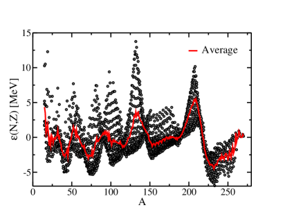
Figure 7: (Colors online) Residuals $\mathcal{E}(N,Z)$ for LD model obtained using least square minimisation. The solid line represents the average residual for fixed values of A as defined in Eq.12.

The variance of the residuals is quite large ($\approx$ few MeV). I tested that the null hypothesis that the residuals are distributed according to a normal distribution is rejected at the 5% level based on the Kolmogorov-Smirnov test  R.J.Barlow (1989). This means that there is a strong signal left in the residuals and Eq.8 is not valid. In this case, I conclude that the model given in Eq.9 is not satisfactory and extra terms should be included to improve the fit Pomorski and Dudek (2003).

III.1 Uncorrelated Bootstrap

I now illustrate how to apply NPB to estimate the parameters of the model in Eq.9 The crucial aspect of NPB is to generate a new series of residuals $\mathcal{E}^{*}(A)$ from random sampling the original one $\mathcal{E}(A)$ and use them to generate a new set of observables (in this case the binding energy) as

$$B^{*}_{exp}(N,Z)=B_{exp}(N,Z)+\mathcal{E}^{*}(N,Z)\;,$$ (11)

and then use $B_{exp}(N,Z)^{*}$ as a new input for a LS minimisation. This is only one possible variant of NPB, for more details I refer to Ref. Efron and Tibshirani (1994). By performing $5000$ bootstrap samplings I derived the empirical distribution of all parameters. I show in Fig.8 the two and one dimensional distribution of the parameters obtained with NPB. This figure is in excellent agreement with the marginalised likelihood obtained with Markov-Chain Monte Carlo in Ref.Shelley et al. (2018). From the one dimensional histogram I extract the 68% quantile. For the first term of Eq.9, I obtain $a_{v}=15.69_{-0.023}^{0.024}$, these values are in good agreement with the error bars provided in Tab.2. Similarly for the other parameters, the error bars obtained with LS and NPB are in agreement. This means NPB provides the same level of accuracy of a standard LS fitting as already spotted in in Ref. Bertsch and Bingham (2017).

The two-dimensional histograms inform us on possible correlations among parameters. Getting a cigar-shape along the diagonal of the figure means strong correlations, while a circle means low or no correlation. I observe that all LD parameters $a_{v},a_{s},a_{c},a_{a}$ are strongly correlated among each other, while the pairing term $\delta$ is not. In this model, $\delta$ is less constrained compared to other parameters as one can also see from the typical error bars obtained in Tab.2. These results can be compared with the one given in Tab.3. Using the data illustrated in Fig.8, I have been able to extract the full covariance matrix which is in perfect agreement with the one calculated using the Hessian matrix of the $\chi^{2}$ R.J.Barlow (1989). This means I did not make use of any explicit numerical derivative in parameter space.

The covariance matrix it not only useful to provide indication concerning error bars and correlations, but it can also be used to extract useful informations about the geometrical properties of the $\chi^{2}$ surface around the minimum. NPB by construction explores the vicinity of the minimum of Eq.10, thus producing the corner plot shown in fig.8. By analysing this figure, it is possible to assess qualitatively which directions in parameter space are more stiff. I refer to Refs Gutenkunst et al. (2007); Nikšić and Vretenar (2016) for a more detailed discussion on the topic.

$\begin{array}[]{ccccc}\includegraphics[width=78.04842pt,angle={0}]{plots/h1.pdf}&&&&\\ \includegraphics[width=78.04842pt,angle={0}]{plots/f11.pdf}&\includegraphics[width=78.04842pt,angle={0}]{plots/h2.pdf}&&&\\ \includegraphics[width=78.04842pt,angle={0}]{plots/f12.pdf}&\includegraphics[width=78.04842pt,angle={0}]{plots/f21.pdf}&\includegraphics[width=78.04842pt,angle={0}]{plots/h3.pdf}&&\\ \includegraphics[width=78.04842pt,angle={0}]{plots/f13.pdf}&\includegraphics[width=78.04842pt,angle={0}]{plots/f22.pdf}&\includegraphics[width=78.04842pt,angle={0}]{plots/f31.pdf}&\includegraphics[width=78.04842pt,angle={0}]{plots/h4.pdf}&\\ \includegraphics[width=78.04842pt,angle={0}]{plots/f14.pdf}&\includegraphics[width=78.04842pt,angle={0}]{plots/f23.pdf}&\includegraphics[width=78.04842pt,angle={0}]{plots/f32.pdf}&\includegraphics[width=78.04842pt,angle={0}]{plots/f41.pdf}&\includegraphics[width=78.04842pt,angle={0}]{plots/h5.pdf}\\ \end{array}$

Figure 8: One and two dimensional histograms of the LD model parameters obtained with NPB assuming uncorrelated residuals. The colour code of the 2-dimensional histogram is an heat-map. The total number of counts is fixed for all the plots $N_{Boot}=5000$. See text for details.

III.2 Block-Bootstrap

As seen in Fig.7, ignoring the autocorrelation between residuals is quite a major approximation. In this section, I illustrate how to correct the NPB to take into account correlations in a simple way.

As a first step, I observe that the variation in the direction N+Z is much more important than in the direction N-Z, so I define an average residual as

$$\mathcal{E}_{A}(A)=\frac{1}{N_{A}}\sum_{Z+N=A}\mathcal{E}(N,Z)\;.$$ (12)

The result is reported in Fig.7 as a solid line. The averaging is not washing out the signal in the data and it is used to simplify the bootstrap treatment. The information along the variation in the N-Z is kept in as an isotopic-dependent variance function defined as

$$\sigma^{2}_{A}=\frac{1}{N_{A}}\sum_{Z+N=A}\left(\mathcal{E}(N,Z)-\mathcal{E}_{A}(A)\right)^{2}\;.$$ (13)

I start determining the degree of correlation between data, by drawing a lag-plot. This is a well know technique to analyse correlation in time series Brockwell and Davis (2013). The lag-plot of lag-$p$ consists in plotting the series against itself, but shifted by $p$ units. In case of non-correlated residues the lag-plot should not show any pattern, i.e one should observe a cloud of points. In Fig. 9 (left panel), I show the lag-1 plot of the averaged residuals. I observe the residuals cluster around the diagonal thus showing a strong autocorrelation.

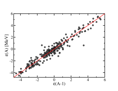
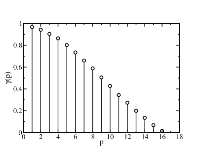
Figure 9: (Colors online) Left panel: lag-plot of order 1 . Right panel: evolution of the self-correlation coefficient defined in Eq.14 for different values of the lag.

To quantify the correlation, I define a self-correlation coefficient as Brockwell and Davis (2013)

$$\gamma(p)=\frac{\sum_{i}(X_{i}-\bar{X})(Y_{i}-\bar{Y})}{\sigma_{x}\sigma_{y}}\;,$$ (14)

where $Y_{i}=X_{i-p}$ is the delayed series. In Fig.9 (right panel), I present the value of such a coefficients for different lags. I observe that there is a non-negligible correlation (i.e. $\gamma(p)\geq 0.5$) up to $p\approx 8$; this means that the residual of a nucleus $A$ is strongly correlated with all other residuals within the interval $[A-8,A+8]$. This is in contradiction with the assumption made in Eq.10, where the $\sigma^{2}$ matrix is assumed to be diagonal.

To take into account the presence of a signal in the residuals, one needs to introduce a minor modification to NPB. Following Ref. Kreiss and Lahiri (2012), instead of resampling individual residuals, I do re-sample blocks of fixed size to preserve the correlations between data. This procedure is named Block Bootstrap (BB).

Given a data-set composed by $n$ elements $\{X_{1},X_{2},\dots,X_{n}\}$, I consider an integer $l$ satisfying $1\leq l\leq n$. I define $\mathcal{B}_{N}$ overlapping blocks of length $l$ as

$$\mathcal{B}_{1} = (X_{1},X_{2},\dots,X_{l})$$

$$\mathcal{B}_{1} = \phantom{X_{1}}(X_{2},X_{3},\dots,X_{l+1})$$

$$\dots = \phantom{(X_{1},X_{2},\dots,X_{l})}\dots$$

$$\mathcal{B}_{N} = \phantom{(X_{1},X_{2},\dots,X_{l}),\dots}(X_{n-l+1},\dots,X_{n})$$

where $N=n-l+1$. The uncorrelated version of bootstrap discussed in previous section is a particular case of BB when $l=1$. In this case there is no overlap between blocks and one should not use BB terminology for such a case. I now treat the different blocks $\mathcal{B}_{N}$ as independent and I thus apply the standard bootstrap algorithm to them. Once the new residuals are produced, I restore the explicit ($N,Z$) dependence by adding an additional error extracted from a Gaussian distribution with variance $\sigma^{2}(A)$ and defined in Eq.13. This is the same procedure followed in Ref. Bertsch and Bingham (2017) in the case of Frequency Domain Bootstrap (FDB).

The choice of $l$ is somehow arbitrary, but in the present case case, I use the lag-plot as indication: I observe that data are correlated over an extension of at least 8 units. I have performed a test on the LD model using BB and various values of the length $l$ of the block.

In Fig.10, I report the experimental distribution obtained using BB for the $a_{v}$ parameter as a function of the size of the block.

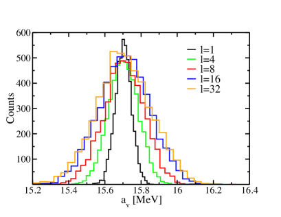
Figure 10: (Colors online) Distribution of the $a_{v}$ parameter obtained using BB and different length of the block. See text for details.

By increasing the size of the blocks, I observe that the distributions gets wider and wider thus showing that I’m taking into account the effect of correlations. I see that $l=8$ captures quite well the correlations, and beyond $l=16$ the distribution does not change anymore. This is due to the fact that the size of the blocks is getting bigger than the size of the correlations. Such a result confirms the outcomes of the lag-plot shown in Fig.9.

From the distributions, I now extract the new error bars of the parameters using the 68% quantile definition. The results are reported in Tab.4. For simplicity I defined the errors to be symmetric around the mean value. This is a minor approximation that has no effect on my conclusions.

Parameter	[MeV]	Error [MeV]
$a_{v}$	15.70	$\pm$0.14
$a_{s}$	17.82	$\pm$0.44
$a_{c}$	0.713	$\pm$0.009
$a_{a}$	23.20	$\pm$0.35
$\delta$	11.78	$\pm$0.80

Table 4: Parameters of LD models obtained using BB and $l=16$.

I observe that the errors are more important using this method and they are most likely more realistic than the one obtained in Tab.2. The only exception is the error on $\delta$ parameter which remains more or less constant. This is related to the fact that it is weakly correlated with the other terms. See Tab.3. The BB does not change the structure of correlations, the results of a corner plot for BB case are quite similar to the ones shown in Fig.8. These results are in good agreement with the one reported in Ref. Bertsch and Bingham (2017) using FDB. Since the covariance matrix changes due to the effect of correlation, this affects the error propagation of the model. For example the error on the binding energy of ²⁰⁸Pb when I use standard bootstrap is $\pm 110$ keV, while when I use BB I obtain $\pm 670$ keV, thus a factor of 6 larger. It would be now interesting to apply BB to more realistic models as the ones presented in Refs Pomorski and Dudek (2003); Duflo and Zuker (1995) to study how error propagation Toivanen et al. (2008); McDonnell et al. (2015) of model parameters is affected.

IV Conclusions

In the present article, I have discussed in detail bootstrap methods and how they can be used to quantify uncertainties for statistical estimators. In particular, I have shown how the minimal hypothesis behind NPB provides a better understanding of the data-set under investigation. The NPB is consistent with findings based on other methods, but it has the remarkable advantage of being able to spot possible outliers in the data-set in a very simple way, without visual investigation of the data. This feature may have interesting application in the case of automatised statistical analysis.

In Se.III, I have shown how NPB can be used to fit parameters of a model, giving at the same time a reasonable estimation of errors and correlations without performing explicitly derivative in parameter space. Contrary to the standard parabolic approximation used to derive errors in a MLE method, the NPB explores the surroundings of the minimum in hyper-parameter space, thus having the possibility of finding possible defects in the hyper-surface.

To take properly into account correlations, I have also discussed a variant of NPB named Block Bootstrap. I have proved that such a method has the same quality of results of Frequency Domain Bootstrap  Bertsch and Bingham (2017), but having the advantage on not using an explicit Fourier transformation of the data and thus potentially being computationally faster. I have also highlighted that the main feature of BB and FDB is that they do not require an explicit modelling of correlations by introducing an ad-hoc covariance matrix into the fit.

Appendix A Infinite matter properties

I report here the explicit nuclear models used in my analysis together with their basic infinite nuclear matter properties. I refer the reader to Refs. Dutra et al. (2012); Sellahewa and Rios (2014); Dutra et al. (2014); Davesne et al. (2016) for more details on the definition of infinite matter properties and how they relate to the parameters of the functionals.

	$\rho_{0}$ [fm-3]	$J_{0}$ [MeV]	$L_{0}$ [MeV]		$\rho_{0}$ [fm-3]	$J_{0}$ [MeV]	$L_{0}$ [MeV]
BSK16 Chamel et al. (2008)	0.159	30.00	34.88	SKA25S20 Dutra et al. (2012)	0.161	33.78	63.82
BSK18 Chamel and Goriely (2010)	0.159	30.00	36.22	SKB Köhler (1976)	0.155	23.89	47.56
BSK19 Goriely et al. (2010)	0.160	30.00	31.9	SKM Krivine et al. (1980)	0.160	30.75	49.36
BSK20 Goriely et al. (2010)	0.160	30.00	37.39	SKM* Bartel et al. (1982)	0.160	30.03	45.78
BSK21 Goriely et al. (2010)	0.158	30.13	46.97	SKRA Rashdan (2000)	0.159	31.32	53.05
BSK22 Goriely et al. (2013)	0.158	32.00	68.49	SKS1 Gómez et al. (1992)	0.161	28.75	30.52
BSK23 Goriely et al. (2013)	0.158	31.00	57.77	SKS3 Gómez et al. (1992)	0.161	28.84	51.74
BSK24 Goriely et al. (2013)	0.158	30.00	46.40	SLYMR1 Sadoudi et al. (2013)	0.155	33.34	49.84
BSK25 Goriely et al. (2013)	0.159	29.00	36.90	SKSC10 Onsi et al. (1994)	0.161	28.11	0.21
BSK26  Goriely et al. (2013)	0.159	30.00	37.49	SKT Ko et al. (1974)	0.148	24.90	28.27
F+ Lesinski et al. (2006)	0.162	32.00	41.54	SKT1 Tondeur et al. (1984)	0.161	32.02	56.19
F-  Lesinski et al. (2006)	0.162	32.00	43.79	SKT1A Dutra et al. (2012)	0.161	32.02	56.20
F0  Lesinski et al. (2006)	0.162	32.00	42.41	SKT5 Tondeur et al. (1984)	0.164	37.00	98.50
KDE  Agrawal et al. (2005)	0.164	31.97	41.42	SKT5A Dutra et al. (2012)	0.164	37.00	98.50
KDE0V  Agrawal et al. (2005)	0.161	32.98	45.21	SKT9 Tondeur et al. (1984)	0.160	29.76	33.77
KDE0V1 Agrawal et al. (2005)	0.165	34.58	54.69	SKT9A Dutra et al. (2012)	0.160	29.76	33.77
LNS1 Gambacurta et al. (2011)	0.162	29.91	30.93	SKX Brown (1998)	0.155	31.11	33.23
MSK1 Tondeur et al. (2000)	0.157	30.00	33.92	SKXCE Brown (1998)	0.155	30.21	33.67
MSK2 Tondeur et al. (2000)	0.157	30.00	33.35	SKXM Brown (1998)	0.159	31.20	32.09
MSK3 Tondeur et al. (2000)	0.158	27.99	6.83	SLY230A Chabanat et al. (1997)	0.160	31.99	44.33
NRAPR Steiner et al. (2005)	0.161	32.78	59.63	SLY230B Chabanat et al. (1997)	0.160	32.01	45.97
RATP Rayet et al. (1982)	0.160	29.26	32.43	SLY4 Chabanat et al. (1997)	0.160	32.00	45.96
SEFM074 Dutra et al. (2012)	0.160	33.40	88.71	SLY5 Chabanat et al. (1997)	0.161	32.01	48.15
SEFM081 Dutra et al. (2012)	0.161	30.76	79.38	SQMC750	0.171	33.75	64.67
SEFM09 Dutra et al. (2012)	0.161	27.78	69.95	SV Beiner et al. (1975)	0.155	32.82	96.07
SEFM1 Dutra et al. (2012)	0.161	24.81	59.55	V100 Pearson and Goriely (2001)	0.157	28.00	8.73
SGII Van Giai and Sagawa (1981)	0.158	26.83	37.66	D1M  Goriely et al. (2009)	0.164	28.50	24.85
SGOI  Shen et al. (2009)	0.168	45.20	99.76	D1S  Dechargé and Gogny (1980)	0.163	31.12	22.46
SI Vautherin (1972)	0.155	29.25	1.29	DD-PC1 Nikšić et al. (2008)	0.152	33.00	70.00
SIII Giannoni and Quentin (1980)	0.145	28.16	9.91	DD-ME1 Lalazissis et al. (2005)	0.152	33.06	55.53
SKA Köhler (1976)	0.155	32.91	74.62	DD-ME2 Lalazissis et al. (2005)	0.152	32.31	51.39
SN2LO1 Becker et al. (2017)	0.162	31.96	48.89

Table 5: Infinite matter properties of the data-set used in the current analysis.

References

- R.J.Barlow (1989) R.J.Barlow, A Guide to the Use of Statistical Methods in the Physical Sciences (John Wiley, 1989).
- Dobaczewski et al. (2014) J. Dobaczewski, W. Nazarewicz, and P. Reinhard, Journal of Physics G: Nuclear and Particle Physics 41, 074001 (2014).
- Roca-Maza et al. (2015) X. Roca-Maza, N. Paar, and G. Colò, Journal of Physics G: Nuclear and Particle Physics 42, 034033 (2015).
- Efron (1979) B. Efron, Annals of Statistics 7, 1 (1979).
- Efron and Tibshirani (1994) B. Efron and R. J. Tibshirani, An introduction to the bootstrap (CRC press, 1994).
- Davison and Hinkley (1997) A. C. Davison and D. V. Hinkley, Bootstrap methods and their application, vol. 1 (Cambridge university press, 1997).
- Chernick et al. (2011) M. R. Chernick, W. González-Manteiga, R. M. Crujeiras, and E. B. Barrios, in International encyclopedia of statistical science (Springer, 2011), pp. 169–174.
- Manly (2006) B. F. Manly, vol. 70 (CRC press, 2006).
- Chernick (2008) M. R. Chernick, Bootstrap methods: a guide for practitioners and researchers, vol. 1 (Wiley-Interscience, 2008).
- Pérez et al. (2014) R. N. Pérez, J. Amaro, and E. R. Arriola, Physics Letters B 738, 155 (2014).
- Nieves (2000) E. Nieves, J.and Ruiz Arriola, The European Physical Journal A 8, 377 (2000), ISSN 1434-601X.
- Bertsch and Bingham (2017) G. Bertsch and D. Bingham, Physical review letters 119, 252501 (2017).
- Muir et al. (2018) D. Muir, A. Pastore, J. Dobaczewski, and C. Barton, Acta Physica Polonica B 49 (2018).
- Pasquini et al. (2018) B. Pasquini, P. Pedroni, and S. Sconfietti, Physical Review C 98, 015204 (2018).
- Fisher and Hall (1990) N. I. Fisher and P. Hall, Geophysical Journal International 101, 305 (1990).
- Miller (1974) R. G. Miller, Biometrika 61, 1 (1974).
- Tukey (1958) J. Tukey, Ann. Math. Statist. 29, 614 (1958).
- Corey et al. (1998) D. M. Corey, W. P. Dunlap, and M. J. Burke, The Journal of general psychology 125, 245 (1998).
- Centelles et al. (2009) M. Centelles, X. Roca-Maza, X. Viñas, and M. Warda, Phys. Rev. Lett. 102, 122502 (2009), URL http://link.aps.org/doi/10.1103/PhysRevLett.102.122502.
- Roca-Maza et al. (2011) X. Roca-Maza, M. Centelles, X. Viñas, and M. Warda, Phys. Rev. Lett. 106, 252501 (2011), URL http://link.aps.org/doi/10.1103/PhysRevLett.106.252501.
- Perlińska et al. (2004) E. Perlińska, S. Rohoziński, J. Dobaczewski, and W. Nazarewicz, Physical Review C 69, 014316 (2004).
- Dechargé and Gogny (1980) J. Dechargé and D. Gogny, Physical Review C 21, 1568 (1980).
- Bender et al. (2003) M. Bender, P.-H. Heenen, and P.-G. Reinhard, Reviews of Modern Physics 75, 121 (2003).
- Nikšić et al. (2008) T. Nikšić, D. Vretenar, and P. Ring, Physical Review C 78, 034318 (2008).
- Warda et al. (2010) M. Warda, X. Viñas, X. Roca-Maza, and M. Centelles, Phys. Rev. C 81, 054309 (2010), URL http://link.aps.org/doi/10.1103/PhysRevC.81.054309.
- Tarbert et al. (2014) C. Tarbert, D. Watts, D. Glazier, P. Aguar, J. Ahrens, J. Annand, H. Arends, R. Beck, V. Bekrenev, B. Boillat, et al., Physical review letters 112, 242502 (2014).
- Dutra et al. (2012) M. Dutra, O. Lourenço, J. S. Sá Martins, A. Delfino, J. R. Stone, and P. D. Stevenson, Phys. Rev. C 85, 035201 (2012), URL http://link.aps.org/doi/10.1103/PhysRevC.85.035201.
- Shen et al. (2009) Q.-b. Shen, Y.-l. Han, H.-r. Guo, et al., Physical Review C 80, 024604 (2009).
- Reinhard and Flocard (1995) P.-G. Reinhard and H. Flocard, Nuclear Physics A 584, 467 (1995).
- Rubin (1981) D. B. Rubin, The annals of statistics pp. 130–134 (1981).
- Boos and Monahan (1986) D. D. Boos and J. F. Monahan, Biometrika 73, 77 (1986).
- Efron and Stein (1981) B. Efron and C. Stein, The Annals of Statistics pp. 586–596 (1981).
- Jodon (2014) R. Jodon, Ph.D. thesis, Université de Lyon (2014).
- Krane and Halliday (1988) K. S. Krane and D. Halliday, Introductory nuclear physics, vol. 465 (Wiley New York, 1988).
- Wang et al. (2012) M. Wang, G. Audi, A. Wapstra, F. Kondev, M. MacCormick, X. Xu, and B. Pfeiffer, Chinese Physics C 36, 1603 (2012).
- Pérez et al. (2015) R. N. Pérez, J. Amaro, and E. R. Arriola, Journal of Physics G: Nuclear and Particle Physics 42, 034013 (2015).
- Klüpfel et al. (2009) P. Klüpfel, P.-G. Reinhard, T. Bürvenich, and J. Maruhn, Physical Review C 79, 034310 (2009).
- Pomorski and Dudek (2003) K. Pomorski and J. Dudek, Physical Review C 67, 044316 (2003).
- Shelley et al. (2018) M. Shelley, P. Becker, A. Gration, and A. Pastore, arXiv preprint arXiv:1811.09130 (2018).
- Gutenkunst et al. (2007) R. N. Gutenkunst, J. J. Waterfall, F. P. Casey, K. S. Brown, C. R. Myers, and J. P. Sethna, PLoS computational biology 3, e189 (2007).
- Nikšić and Vretenar (2016) T. Nikšić and D. Vretenar, Physical Review C 94, 024333 (2016).
- Brockwell and Davis (2013) P. J. Brockwell and R. A. Davis, Time series: theory and methods (Springer Science & Business Media, 2013).
- Kreiss and Lahiri (2012) J.-P. Kreiss and S. N. Lahiri, in Handbook of statistics (Elsevier, 2012), vol. 30, pp. 3–26.
- Duflo and Zuker (1995) J. Duflo and A. Zuker, Physical Review C 52, R23 (1995).
- Toivanen et al. (2008) J. Toivanen, J. Dobaczewski, M. Kortelainen, and K. Mizuyama, Physical Review C 78, 034306 (2008).
- McDonnell et al. (2015) J. McDonnell, N. Schunck, D. Higdon, J. Sarich, S. Wild, and W. Nazarewicz, Physical review letters 114, 122501 (2015).
- Sellahewa and Rios (2014) R. Sellahewa and A. Rios, Physical Review C 90, 054327 (2014).
- Dutra et al. (2014) M. Dutra, O. Lourenço, S. Avancini, B. Carlson, A. Delfino, D. Menezes, C. Providência, S. Typel, and J. Stone, Physical Review C 90, 055203 (2014).
- Davesne et al. (2016) D. Davesne, A. Pastore, and J. Navarro, Astronomy & Astrophysics 585, A83 (2016).
- Chamel et al. (2008) N. Chamel, S. Goriely, and J. Pearson, Nuclear Physics A 812, 72 (2008).
- Chamel and Goriely (2010) N. Chamel and S. Goriely, Physical Review C 82, 045804 (2010), ISSN 0556-2813.
- Köhler (1976) H. Köhler, Nuclear Physics A 258, 301 (1976).
- Goriely et al. (2010) S. Goriely, N. Chamel, and J. M. Pearson, Phys. Rev. C 82, 035804 (2010), URL https://link.aps.org/doi/10.1103/PhysRevC.82.035804.
- Krivine et al. (1980) H. Krivine, J. Treiner, and O. Bohigas, Nuclear Physics A 336, 155 (1980).
- Bartel et al. (1982) J. Bartel, P. Quentin, M. Brack, C. Guet, and H.-B. Håkansson, Nuclear Physics A 386, 79 (1982).
- Rashdan (2000) M. Rashdan, Modern Physics Letters A 15, 1287 (2000).
- Goriely et al. (2013) S. Goriely, N. Chamel, and J. Pearson, Physical Review C 88, 024308 (2013).
- Gómez et al. (1992) J. Gómez, C. Prieto, and J. Navarro, Nuclear Physics A 549, 125 (1992).
- Sadoudi et al. (2013) J. Sadoudi, M. Bender, K. Bennaceur, D. Davesne, R. Jodon, and T. Duguet, Physica Scripta 2013, 014013 (2013).
- Onsi et al. (1994) M. Onsi, H. Przysiezniak, and J. Pearson, Physical Review C 50, 460 (1994).
- Ko et al. (1974) C. Ko, H. Pauli, M. Brack, and G. Brown, Nuclear Physics A 236, 269 (1974).
- Lesinski et al. (2006) T. Lesinski, K. Bennaceur, T. Duguet, and J. Meyer, Physical Review C 74, 044315 (2006).
- Tondeur et al. (1984) F. Tondeur, M. Brack, M. Farine, and J. Pearson, Nuclear Physics A 420, 297 (1984).
- Agrawal et al. (2005) B. Agrawal, S. Shlomo, and V. K. Au, Physical Review C 72, 014310 (2005).
- Gambacurta et al. (2011) D. Gambacurta, L. Li, G. Colo, U. Lombardo, N. Van Giai, and W. Zuo, Physical Review C 84, 024301 (2011).
- Brown (1998) B. A. Brown, Physical Review C 58, 220 (1998).
- Tondeur et al. (2000) F. Tondeur, S. Goriely, J. Pearson, and M. Onsi, Physical Review C 62, 024308 (2000).
- Chabanat et al. (1997) E. Chabanat, P. Bonche, P. Haensel, J. Meyer, and R. Schaeffer, Nuclear Physics A 627, 710 (1997).
- Steiner et al. (2005) A. W. Steiner, M. Prakash, J. M. Lattimer, and P. J. Ellis, Physics reports 411, 325 (2005).
- Rayet et al. (1982) M. Rayet, M. Arnould, G. Paulus, and F. Tondeur, Astronomy and Astrophysics 116, 183 (1982).
- Beiner et al. (1975) M. Beiner, H. Flocard, N. Van Giai, and P. Quentin, Nuclear Physics A 238, 29 (1975).
- Pearson and Goriely (2001) J. Pearson and S. Goriely, Physical Review C 64, 027301 (2001).
- Van Giai and Sagawa (1981) N. Van Giai and H. Sagawa, Physics Letters B 106, 379 (1981).
- Goriely et al. (2009) S. Goriely, S. Hilaire, M. Girod, and S. Péru, Physical review letters 102, 242501 (2009).
- Vautherin (1972) D. Vautherin, Phys. Rev. C 5, 626 (1972).
- Giannoni and Quentin (1980) M. Giannoni and P. Quentin, Physical Review C 21, 2076 (1980).
- Lalazissis et al. (2005) G. Lalazissis, T. Nikšić, D. Vretenar, and P. Ring, Physical Review C 71, 024312 (2005).
- Becker et al. (2017) P. Becker, D. Davesne, J. Meyer, J. Navarro, and A. Pastore, Physical Review C 96, 044330 (2017).