Non-adiabatic mass-correction functions and rovibrational states of ⁴He${}_{2}^{+}$ ($X\ ^{2}\Sigma_{\text{u}}^{+}$)

Abstract

The mass-correction functions in the second-order non-adiabatic Hamiltonian are computed for the ⁴He${}^{+}_{2}$ molecular ion using the variational method, floating explicitly correlated Gaussian functions, and a general coordinate-transformation formalism. When non-adiabatic rovibrational energy levels are computed using these (coordinate-dependent) mass-correction functions and a highly accurate potential energy and diagonal Born–Oppenheimer correction curve, significantly improved theoretical results are obtained for the nine rotational and two rovibrational intervals known from high-resolution spectroscopy experiments.

I Introduction

Precision spectroscopy measurements challenge theoretical and computational methodologies to go much beyond the current state of the art and to study various possible subtle effects, which have been overlooked or considered to be negligible in the past. The search for “small effects” is usually triggered by a disagreement between the most accurate experimental and the best possible theoretical results, when this disagreement is larger than the error bars on the experimental and computed datasets. A famous example for a decades-long, hand-in-hand race of theory and experiment is the dissociation energy of molecular hydrogen Liu et al. (2009); Sprecher et al. (2011), which started at the advent of quantum mechanics and has reached by now a level of sophistication when experts propose to use the hydrogen molecule’s spectral lines to test fundamental physical constants and search for new physical theories Beyer et al. (2018); Altmann et al. (2018), thereby cultivating a renaissance for molecular physics.

The present work is motivated by the sizeable disagreement between the recently measured rotational intervals of ⁴He${}_{2}^{+}$ Semeria et al. (2016) and adiabatic rotational-vibrational computations using a highly accurate potential energy curve, including the diagonal Born–Oppenheimer corrections (DBOC), obtained with variationally optimized floating explicitly correlated Gaussian (fECG) functions in Ref. Tung et al. (2012). The deviation of the experimental and computational results increases with the rotational quantum number, $N^{+}$, the energy of which is measured from the $N^{+}=1$ rotational state (in the electronic and vibrational ground state). The deviation becomes as large as $0.069$ cm^-1 (2.1 GHz) for the $\tilde{\nu}(N^{+}=19)-\tilde{\nu}(N^{+}=1)$ interval, which is almost twice as large as the estimated relativistic and radiative corrections. Semeria, Jansen, and Merkt proposed Semeria et al. (2016) that the neglect of the coordinate-dependence of the effective masses, which would account for non-adiabatic effects, could be responsible for the “missing” part of the deviation between experiment and theory.

The second-order non-adiabatic Hamiltonian for a single isolated electronic state, which includes a kinetic-energy-correction term that can be written as a correction to the mass tensor, has been discovered and re-discovered in various contexts in the past Fisk and Kirtman (1964); Herman and Asgharian (1966); Bunker and Moss (1977, 1980); Bunker et al. (1977); Weigert and Littlejohn (1993); Aubert-Frecon et al. (1994); Braun et al. (1996); Herman and Ogilvie (1998); Ogilvie (1998); Schwenke (2001a, b); Sauer et al. (2005); Bak et al. (2005); Pachucki and Komasa (2008, 2009); Holka et al. (2011); Pachucki and Komasa (2012); Panati et al. (2007); Scherrer et al. (2017)—for a hopefully nearly complete summary see the Introduction of Ref. Ma (1) (henceforth Paper I). These derivations and discoveries have remained somewhat isolated yet, and the rigorous computation of the mass-correction tensor is rarely carried out, whereas the DBOC, which appears at the same order in the Hamiltonian, is almost routinely computed for a variety of poly-electronic and poly-atomic molecules Handy et al. (1986); Handy and Lee (1996); Ioannou et al. (1996); Valeev and Sherrill (2003). In the present work, we use the general curvilinear formalism and our in-house developed variational fECG code Ma (1) to obtain the rigorous mass-correction functions for the ⁴He${}_{2}^{+}$ molecular ion in its $X\ ^{2}\Sigma_{\text{u}}^{+}$ ground electronic state, and compute its non-adiabatic rovibrational bound and long-lived resonance states.

II Theoretical and computational details

In Paper I we have re-written the second-order non-adiabatic Hamiltonian, $\hat{H}^{\text{(2)}}$, of Ref. Panati et al. (2007), using a general curvilinear coordinate formalism and considered the time-independent Schrödinger equation:

$$\left(-\frac{1}{2}\tilde{g}^{-1/2}\partial_{\mu}\tilde{g}^{1/2}\tilde{G}^{\mu\nu}\partial_{\nu}+U+V\right)\phi=E\phi$$ (1)

where $U$ is the diagonal Born–Oppenheimer correction to the BO potential energy, $V$, and the effective $\tilde{G}^{\mu\nu}$ tensor was written as:

$$\tilde{G}^{\mu\nu} =\frac{1}{{m_{\text{n}}}}g^{\mu\alpha}(\boldsymbol{S}\boldsymbol{I}_{6}\boldsymbol{S}^{\text{T}})_{\alpha\beta}g^{\beta\nu}-\frac{1}{{m_{\text{n}}}^{2}}g^{\mu\alpha}(\boldsymbol{S}\bar{\mathcal{A}}\boldsymbol{S}^{\text{T}})_{\alpha\beta}g^{\beta\nu}$$

$$=\left[\frac{1}{{m_{\text{n}}}}\delta^{\mu}\,_{\beta}-\frac{1}{{m_{\text{n}}}^{2}}\mathcal{A}^{\mu}\,_{\beta}\ \right]g^{\beta\nu}.$$ (2)

In Eq. (2), $g^{\alpha\beta}$ is the $(\alpha,\beta)$th element of the contravariant metric tensor of the curvilinear coordinates and we defined the transformation matrix

$$\boldsymbol{S}=\boldsymbol{J}^{\text{T}}\boldsymbol{O}.$$ (3)

In Eq. (3) $\boldsymbol{J}$ is the Jacobian matrix for the curvilinear coordinates and $\boldsymbol{O}$ is a rotation matrix which connects the laboratory frame and the frame of the atomic nuclei used to compute the elements of the $\bar{\mathcal{A}}$ mass-correction tensor from electronic-structure theory. For a body-fixed frame selected for the atomic nuclei ($R_{ia},\ i=1,\ldots,N$ and $a=x(1),y(2),z(3)$) $\bar{\mathcal{A}}$ is computed as

$$\bar{\mathcal{A}}_{ia,jb}(\boldsymbol{R}) =2\langle\partial_{R_{ia}}\psi|(\hat{H}_{\text{el}}-E)^{-1}(1-\hat{P})\partial_{R_{jb}}\psi\rangle_{\text{el}}$$

$$\approx 2\sum_{n=1}^{N_{\text{aux}}}\sum_{m=1}^{N_{\text{aux}}}\langle\partial_{R_{ia}}\psi|f_{n}\rangle_{\text{el}}\left(\boldsymbol{F}^{-1}\right)_{nm}\langle f_{m}|\partial_{R_{jb}}\psi\rangle_{\text{el}}$$ (4)

with

$$(\boldsymbol{F})_{nm}(E)=\langle f_{n}|(\hat{H}_{\text{el}}-E)(1-\hat{P})|f_{m}\rangle_{\text{el}},$$ (5)

and we have introduced the $\{f_{n},n=1,\ldots N_{\text{aux}}\}$ auxiliary basis set to compute the resolvent. $1-\hat{P}$ is a projector to the space orthogonal to the electronic state $\psi$, which is an “isolated” eigenstate of the $\hat{H}_{\text{el}}$ electronic Hamiltonian, for further details see Paper I.

Derivatives of the electronic wave functions are computed by finite differences with a step size of $\Delta=10^{-4}$ bohr along each Cartesian directions and using the rescaling idea for the fECG centers upon a small change of the nuclear positions Cencek and Kutzelnigg (1997); Ma (1). Instead of directly computing $\boldsymbol{F}^{-1}$, we solve the system of linear equations for $\boldsymbol{x}_{m,j_{b}}$

$$[\boldsymbol{F}(E+\text{i}\varepsilon)\ \boldsymbol{x}_{j_{b}}]_{m}=\langle f_{m}|\partial_{R_{jb}}\psi\rangle_{\text{el}},$$ (6)

where instead of using $E$, we have $E+\text{i}\varepsilon$ which allows us to avoid the implicit or explicit inversion of a near singular matrix ($E$ is a tight variational upper bound to an eigenvalue of the electronic Hamiltonian, $\hat{H}_{\text{el}}$). For the present applications, $\text{i}\varepsilon=\text{i}10^{-3}-\text{i}10^{-5}$ E${}_{\text{h}}$ ensured numerically stable results (mass-correction values) over the $\rho\in[1,10]$ bohr internuclear distance interval to at least 4 significant digits (for $\rho>10$ bohr we have approximated the mass-correction functions with their asymptotic value, see Fig. 1).

For homonuclear diatomic molecules, it is natural to replace the six Cartesian coordinates with the three polar coordinates, $(\rho,\theta,\phi)$ and the three Cartesian coordinates of the nuclear center of mass (NCM). This transformation and the particular expressions for the effective $\tilde{G}^{\mu\nu}$ tensor have been worked out in detail in Paper I, so we only repeat the final expression (“.” means “0” in the matrix):

$$\tilde{G}^{\mu\nu} ={\tiny\left(\begin{array}[]{@{}c@{}c@{}c | c@{}c@{}c @{}}\frac{2}{m_{\text{n}}}\left[1-\frac{\mathcal{A}^{\rho}\,_{\rho}}{m_{\text{n}}}\right]&.&.&.&.&.\\ .&\frac{2}{m_{\text{n}}}\left[1-\frac{\mathcal{A}^{\theta}\,_{\theta}}{m_{\text{n}}}\right]\frac{1}{\rho^{2}}&.&.&.&.\\ .&.&\frac{2}{m_{\text{n}}}\left[1-\frac{\mathcal{A}^{\phi}\,_{\phi}}{{m_{\text{n}}}}\right]\frac{1}{\rho^{2}\sin^{2}\theta}&.&.&.\\ \cline{1-6}\cr.&.&.&&&\\ .&.&.&\lx@intercol\hfil\frac{1}{2m_{\text{n}}}\left[1-\frac{\mathcal{A}^{\text{NCM}}\ _{\text{NCM}}}{{m_{\text{n}}}}\right]\boldsymbol{I}_{3}\hfil\lx@intercol\\ .&.&.&&&\\ \end{array}\right)}$$ (13)

It is important to re-iterate that not only in the BO, $\hat{H}^{\text{(0)}}$, but also in $\hat{H}^{\text{(2)}}$, the translation of the nuclear center of mass (always) exactly separates from the translationally invariant (TI), i.e., rotational-vibrational, part of the problem (in $\tilde{G}^{\mu\nu}$ the TI-NCM block is rigorously zero) Scherrer et al. (2017), hence we consider only the rovibrational part by subtracting the translational kinetic energy of the center of mass (which also gains a correction term in $\hat{T}^{\text{(2)}}$). Furthermore, the kinetic energy operator of diatomic molecules ($\hat{T}^{(0)}$ or $\hat{T}^{(2)}$) does not contain any mixed derivatives between the radial and angular coordinates (note that the TI block in Eq. (13) is diagonal). Hence, the angular part of the second-order rovibrational Hamiltonian can be integrated with the $Y_{JM}(\theta,\phi)$ spherical harmonic functions (similarly to the standard solution of diatomics with $\hat{T}_{\text{rv}}^{(0)}$), and we are left with the numerical solution of the radial equation:

$$\left(-\frac{1}{2}\frac{1}{\rho^{2}}\frac{\partial}{\partial\rho}\rho^{2}\frac{2}{m_{\text{n}}}\left[1-\frac{\mathcal{A}^{\rho}\,_{\rho}}{m_{\text{n}}}\right]\frac{\partial}{\partial\rho}\right.$$

$$+\left.\frac{J(J+1)}{\rho^{2}}\frac{1}{m_{\text{n}}}\left[1-\frac{\mathcal{A}^{\Omega}\,_{\Omega}}{m_{\text{n}}}\right]+U(\rho)+V(\rho)\right)\varphi_{J}(\rho)=E_{J}\varphi_{J}(\rho)$$ (14)

where $\varphi_{J}$ is normalized using the volume element $\rho^{2}\text{d}\rho$. Instead of solving Eq. (14), we proceed similarly to Pachucki and Komasa Pachucki and Komasa (2009) and use the operator identity

$$\frac{1}{\rho^{2}}\frac{\partial}{\partial\rho}\rho^{2}X(\rho)\frac{\partial}{\partial\rho}=\frac{1}{\rho}\frac{\partial}{\partial\rho}X(\rho)\frac{\partial}{\partial\rho}\rho-\frac{1}{\rho}\frac{\partial X(\rho)}{\partial\rho}$$ (15)

to obtain

$$\left(-\frac{\partial}{\partial\rho}\frac{1}{m_{\text{n}}}\left[1-\frac{\mathcal{A}^{\rho}\,_{\rho}}{m_{\text{n}}}\right]\frac{\partial}{\partial\rho}\right.$$

$$\left.-\frac{1}{\rho}\frac{1}{m_{\text{n}}^{2}}\frac{\partial\mathcal{A}^{\rho}\,_{\rho}}{\partial\rho}+\frac{J(J+1)}{\rho^{2}}\frac{1}{m_{\text{n}}}\left[1-\frac{\mathcal{A}^{\Omega}\,_{\Omega}}{m_{\text{n}}}\right]+U(\rho)+V(\rho)\right)\chi_{J}(\rho)=E_{J}\chi_{J}(\rho),$$ (16)

where $\chi_{J}(\rho)=\rho\varphi_{J}(\rho)$ and $\chi_{J}$ is normalized with the volume element $\text{d}\rho$. To obtain rovibrational energies (including non-adiabatic corrections) and wave functions, we solve Eq. (16) using the discrete variable representation (DVR) and associated Laguerre polynomials, $L_{n}^{(\alpha)}$ with $\alpha=2$ for the radial (vibrational) degree of freedom. The DVR points are scaled to an $[R_{\text{min}},R_{\text{max}}]$ interval. The $n$ number of DVR points and functions, as well as $R_{\text{min}}$ and $R_{\text{max}}$ are determined as convergence parameters, and their typical value is around $n=300-1000$, $R_{\text{min}}=1$ bohr and $R_{\text{max}}=30-100$ bohr. Finally, we mention that the term including the $\partial\mathcal{A}^{\rho}\,_{\rho}/\partial\rho$ derivative has an almost negligible effect on the computed rotational-vibrational states ($<0.001$ cm^-1).

II.1 Mass-correction curves and non-adiabatic rovibrational energies

For the rovibrational computations, we used the highly accurate PES and DBOC curves computed by Tung, Pavanello, and Adamowicz Tung et al. (2012). The mass-correction functions have been evaluated in the present work using a modified version of our in-house developed pre-Born–Oppenheimer (preBO) code Mátyus et al. (2011a, b); Mátyus and Reiher (2012); Mátyus (2013, 2018), see also related developments in Refs. Simmen et al. (2013a, 2014, b); Muolo et al. (2018). The particular computational methodology for the mass-correction tensor is explained in Paper I, and the numerical details for the present system are described in the following paragraphs.

We optimized the floating ECG basis function parameters as well as the single parameter in the spin function of three electrons coupled to a doublet state Suzuki and Varga (1998) by minimizing the electronic energy at the internuclear distance $\rho=2$ bohr. The electronic energy was converged within $10\ \mu$$E_{\text{h}}$ ($\sim 2.2$ cm^-1) in comparison with earlier work Cencek and Rychlewski (1995); Tung et al. (2012). Starting out from the optimized electronic basis set corresponding to $\rho=2$ bohr, we have increased (and decreased) the internuclear distance step by step with $\Delta\rho=0.1$ bohr to cover the $\rho\in[1,10]$ bohr interval. At each step, we have rescaled the basis set origins Cencek and Kutzelnigg (1997) and performed an entire refinement cycle of the non-linear parameters. This rescaled and refined basis set was used for making the next step along the series of nuclear configurations (the refinement was necessary in order to maintain the accuracy of the results after making several nuclear displacements). The resulting basis sets provided us with an electronic energy accurate within ca. 10–15 $\mu$$E_{\text{h}}$ over the $\rho\in[1,10]$ bohr interval. We have carried out a variety of convergence tests for the mass correction functions with respect to (a) the convergence of the electronic state wave function, $\psi$; and (b) the size of the auxiliary basis set used to express the resolvent, Eqs. (4)–(5). A quick assessment of the auxiliary basis set was possible based on the observation that the mass correction terms were inaccurate if the insertion of the truncated resolution of identity in the derivative overlaps gave inaccurate results (see Sec. IVB of Paper I). The auxiliary basis set of increasing size was compiled from the basis sets optimized for the electronic wave functions at neighboring nuclear configurations: $\rho$, $\rho\pm 0.1$ bohr, $\rho\pm 0.2$ bohr, $\rho\pm 0.3$ bohr. The computed mass-correction functions for the radial and angular degrees of freedom, $\delta\tilde{m}_{\text{vib}}=\mathcal{A}^{\rho}\,_{\rho}$ and $\delta\tilde{m}_{\text{rot}}=\mathcal{A}^{\Omega}\,_{\Omega}$, respectively, are visualized in Figure 1 (the numerical values are deposited in the Supplementary Material).

The first nine rotational intervals measured from the $N^{+}=1$ rotational state (in the electronic and vibrational ground state) of ⁴He${}_{2}^{+}$ are given in Table 1 (in what follows, we adopt the notation of Ref. Semeria et al. (2016) and use $N^{+}$ for the rotational angular momentum quantum number of He${}_{2}^{+}$). For a direct comparison with the experimentally observed rotational intervals, we added to the non-adiabatic transition energies the estimated relativistic and radiative corrections Tung et al. (2012). According to the explanation in Ref. Semeria et al. (2016) these corrections were calculated by scaling the relativistic and radiative corrections of the rotational states of H₂ Piszczatowski et al. (2009) by a factor of 3.9.

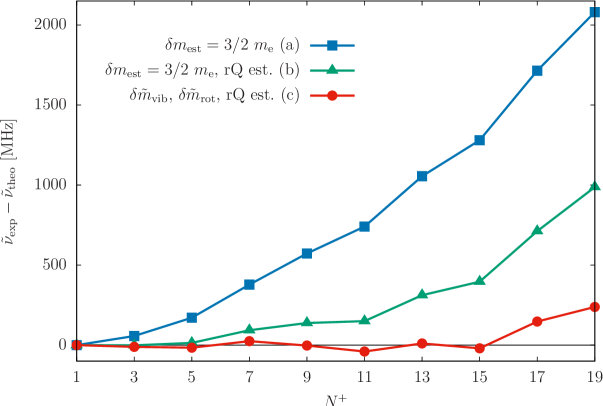
Figure 2: Deviation of the experimentally measured Semeria et al. (2016) and computed rotational transitions of the ⁴He${}_{2}^{+}$ molecular ion in its ground electronic and vibrational state ($X\ ^{2}\Sigma_{\text{u}}^{+}$, $v=0$). The rotational intervals were computed using the PES and DBOC curves of Ref. Tung et al. (2012) and (a) the $\delta m_{\text{est}}=3/2$ constant-mass correction model also used in Ref. Tung et al. (2012) (blue squares); (b) the same as (a) but including the relativistic and radiative estimates Tung et al. (2012), see text and Ref. Semeria et al. (2016) for details (green triangles); and (c) using the rigorous mass-correction functions computed in the present work and including the relativistic and radiative estimates (red circles).

The deviation of the computed rotational intervals from experiment is visualized in Figure 2. In particular for high rotational angular momentum values the explicit inclusion of the rotational and vibrational mass curves significantly improves the agreement with the experimental results in comparison with the naïve choice of an effective mass including the 3/2 mass of an electron (an equal share of the mass of the three electrons between the two atomic nuclei).

In order to attach error bars to our computational results, we can think about the following possible sources of errors and inaccuracies. By repeating the evaluation of the mass-correction functions using an increasing number of electronic and auxiliary basis functions, we estimate that the $\mathcal{A}^{\rho}\,_{\rho}$ and $\mathcal{A}^{\Omega}\,_{\Omega}$ values are converged to within about 0.1–0.5 % (see also Paper I for the numerical and convergence properties of the mass-correction functions of H${}_{2}^{+}$). A 1 % change of the rotational mass correction function ($1\pm 0.01$ $\mathcal{A}^{\Omega}\,_{\Omega}$) results in a $\pm 0.005$ cm^-1 change in the $\Delta\tilde{\nu}(N^{+}=19)-\tilde{\nu}(N^{+}=1)$ interval (for lower $N^{+}$ upper states the change is smaller). So, the uncertainty of the non-adiabatic rotational intervals with respect to the enlargement of the electronic and auxiliary basis sets is probably smaller than this value. The pure rotational intervals measured in Ref. Semeria et al. (2016) are not sensitive to inaccuracies in the vibrational mass correction function (a $\pm 50$ % change of $\mathcal{A}^{\rho}\,_{\rho}$ results in a $\mp 0.001$ cm^-1 change in $\Delta\tilde{\nu}=\tilde{\nu}(N^{+}=19)-\tilde{\nu}(N^{+}=1)$).

It is much more difficult for us to make an assessment about the error in the estimated relativistic and radiative corrections, and firm error bounds could be made by explicitly computing these corrections for the ⁴He${}_{2}^{+}$ molecular ion.

To finish with the discussion of the numerical results, we comment on the two earlier ⁴He${}_{2}^{+}$ measurements Maas et al. (1976); Carrington et al. (1995). Ref. Maas et al. (1976) reported predissociative features of ⁴He${}_{2}^{+}$. In the hope of being able to identify (and assign) the reported peaks we computed “all” bound and long-lived resonance states of ⁴He${}_{2}^{+}$ using the rigorous mass-correction curves computed in this work and the highly accurate PES and DBOC curves of Ref. Tung et al. (2012). Due to the low resolution and relatively large uncertainty of the experimental energy positions of Maas et al. (1976), we refrain here from giving any suggestions for the assignment, and just deposit the computed non-adiabatic rovibrational energies (and non-adiabatic corrections) in the Supplementary Material.

Using the high-resolution microwave electronic transitions reported in Ref. Carrington et al. (1995), two rovibrational energy intervals of the ground-electronic state can be deduced. These intervals were computed in Ref. Tung et al. (2012) with the constant $\delta m=3/2\ m_{\mathrm{e}}$ mass correction model, and we have also computed them with the coordinate-dependent mass functions (see Table 2). The $(v,N^{+})=(23,3)-(23,1)$ interval was obtained in excellent agreement with the experiments already with the constant mass model Tung et al. (2012) and a similarly excellent agreement is observed using the rigorous mass-correction functions. For the $(v,N^{+})=(23,3)-(22,5)$ interval the authors of Ref. Tung et al. (2012) observed a larger, 0.012 cm^-1, deviation from experiment. When using the rigorous mass functions, this deviation is reduced to $-0.003$ cm^-1, which is probably in the order of magnitude of the relativistic and radiative corrections, which (as explained earlier) should be addressed in future work.

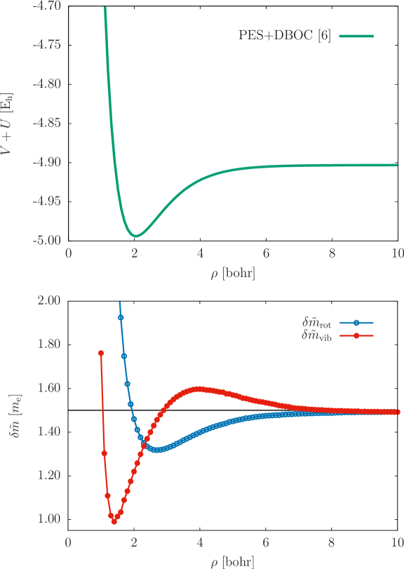
Figure 1: ⁴He${}_{2}^{+}$ molecular ion in its $X\ {{}^{2}\Sigma}_{\text{u}}^{+}$ (ground) electronic state: rotational, $\delta\tilde{m}_{\text{rot}}=\mathcal{A}^{\Omega}\,_{\Omega}$ and vibrational, $\delta\tilde{m}_{\text{vib}}=\mathcal{A}^{\rho}\,_{\rho}$ mass-correction functions computed in the present work. The thin line takes the constant value of $3/2=1.5\ m_{\text{e}}$, which corresponds to an equal share of the three electrons between the two atomic nuclei. The adiabatic PES curve (upper plot) is reproduced using the points of Ref. Tung et al. (2012) to show the value and change of the mass-correction functions with respect to the PES valley.

Table 1: Comparison of the experimentally measured and computed rotational intervals, in cm^-1, of the ⁴He${}_{2}^{+}$ ion in its electronic and vibrational ground state ($X\ {{}^{2}\Sigma}_{\text{u}}^{+}$, $v=0$). In all computations we used the highly accurate PES and DBOC curves computed by Tung et al. Tung et al. (2012). The nuclear mass for the ⁴He nucleus was $m_{\text{n}}=7\,294.299\,536\,3\ m_{\text{e}}$ (same as in Ref. Tung et al. (2012)) and $1~{}\mathrm{E}_{\mathrm{h}}=219\,474.6313\,702$ cm^-1 cod .

$N^{+}$	$\tilde{\nu}_{\text{exp}}$ ${}^{\text{a}}$	$\tilde{\nu}_{\text{na-est}}$	($\delta\tilde{\nu}_{\text{na-est}}$) ${}^{\text{b}}$		$\tilde{\nu}_{\text{na}}$	($\delta\tilde{\nu}_{\text{na}}$) ${}^{\text{c}}$		$\tilde{\nu}_{\text{na-rQest}}$	($\delta\tilde{\nu}_{\text{na,rQ-est}}$) ${}^{\text{d}}$
		$[\delta m_{\text{est}}=3/2m_{\text{e}}]$			$[\delta\tilde{m}_{\text{rot}},\delta\tilde{m}_{\text{vib}}]$			$[\delta\tilde{m}_{\text{rot}},\delta\tilde{m}_{\text{vib}},\text{rQ est.}]$
1	0	0			0			0
3	70.9379	70.936	(0.002)		70.936	(0.002)		70.938	(0.000)
5	198.3647	198.359	(0.006)		198.360	(0.005)		198.365	($-0.001$)
7	381.8346	381.822	(0.013)		381.824	(0.010)		381.834	(0.001)
9	620.7021	620.683	(0.019)		620.688	(0.014)		620.702	(0.000)
11	914.1367	914.112	(0.025)		914.118	(0.018)		914.138	($-0.001$)
13	1261.1242	1261.089	(0.035)		1261.099	(0.025)		1261.124	(0.000)
15	1660.4627	1660.420	(0.043)		1660.434	(0.029)		1660.463	($-0.001$)
17	2110.7932	2110.736	(0.057)		2110.755	(0.038)		2110.788	(0.005)
19	2610.5744	2610.505	(0.069)		2610.530	(0.044)		2610.566	(0.008)

${}^{\text{a}}$: Experimental results taken from Table I of Ref. Semeria et al. (2016).

${}^{\text{b}}$: Rotational intervals computed with constant effective nuclear masses corresponding to the qualitative reasoning that the electrons follow the nuclei: $m_{\text{est}}=m_{\text{n}}+\delta m_{\text{est}}$ (both for rotations and vibrations). These effective masses were used also in Ref. Tung et al. (2012) to compute rotation-vibration energy levels.

${}^{\text{c}}$: Rotational intervals computed with the rigorous mass-correction functions computed in the present work (see Figure 1).

${}^{\text{d}}$: Rotational transitions obtained in ${}^{\text{c}}$ corrected with the estimated relativistic and radiative effects for each rotational state according to Ref. Tung et al. (2012) (see also text and Ref. Semeria et al. (2016) for details).

Table 2: Comparison of rovibrational transition energies of ⁴He${}_{2}^{+}$ derived from experiment Carrington et al. (1995) and computed with the adiabatic potential energy curve of Ref. Tung et al. (2012) and constant effective masses ($\tilde{\nu}_{\text{na-est}}$) as well as with the rigorous mass-correction curves ($\tilde{\nu}_{\text{na}}$) computed in this work.

$(v^{\prime},{N^{+}}^{\prime})$	$(v^{\prime\prime},{N^{+}}^{\prime\prime})$	$\tilde{\nu}_{\text{exp}}$${}^{\text{a}}$	$\tilde{\nu}_{\text{na-est}}$ ($\delta\tilde{\nu}_{\text{na-est}}$) ${}^{\text{b}}$			$\tilde{\nu}_{\text{na}}$ ($\delta\tilde{\nu}_{\text{na}}$) ${}^{\text{c}}$
			$[\delta m_{\text{est}}=3/2m_{\text{e}}]$			$[\delta\tilde{m}_{\text{rot}},\delta\tilde{m}_{\text{vib}}]$
(23,3)	(22,5)	5.248	5.260	$(0.012)$		5.250	$(-0.002)$
(23,3)	(23,1)	2.001	2.002	$(0.001)$		1.999	$(0.002)$

${}^{\text{a}}$: Experimental results of Ref. Carrington et al. (1995).

${}^{\text{b}}$: See footnote (b) to Table 1.

${}^{\text{c}}$: See footnote (c) to Table 1.

III Summary and conclusions

We have computed the rigorous rotational and vibrational mass-correction functions in the second-order non-adiabatic Hamiltonian Panati et al. (2007) for the ⁴He${}_{2}^{+}$ molecular ion in its $X\ ^{2}\Sigma_{\text{u}}^{+}$ (ground) electronic state. The computations have been carried out using the variational method and floating explicitly correlated Gaussian functions and a general curvilinear formalism of the second-order kinetic-energy operator including the mass-correction tensor developed in Ref Ma (1). Solution of the rovibrational time-independent Schrödinger equation including the computed, rigorous, non-adiabatic mass-correction functions results in a promising improvement in comparison with experimental results. If estimates for the relativistic and radiative corrections Tung et al. (2012) are also included, deviation of the rotational intervals, $\tilde{\nu}(N^{+})-\tilde{\nu}(1)$ (with $N^{+}=3,5,$…,19) is reduced to less than 100 MHz for up to $N^{+}=15$, which increases to 240 MHz for $N^{+}=19$. In order to be able to attach rigorous error bars (and a possible improvement for $N^{+}\geq 17)$ to the theoretical results, it will be necessary to explicitly compute the relativistic and radiative corrections for ⁴He${}_{2}^{+}$. At the present stage, we may conclude that the highly accurate PES and DBOC points of Ref. Tung et al. (2012) and the series of high-precision rotational intervals measured in Semeria et al. (2016) made it possible to study and identify subtle non-adiabatic effects in one of the simplest poly-electronic molecule (molecular ion).

Note added at the revision stage
After submission of this work, we became aware of new measurements which determine rotational intervals for the first vibrational excitation ($v=1$) and the vibrational fundamental frequency of ⁴He${}_{2}^{+}$ JaS . The increasing experimental dataset will allow a more detailed study of the fine interplay of small effects earlier neglected in the theoretical description of this molecular ion.

Supplementary Material
The Supplementary Material contains 1) non-adiabatic rovibrational energies obtained with the rigorous mass-correction functions; 2) deviation of the rovibrational energies computed with the non-adiabatic mass-correction functions and constant masses (nuclear plus 3/2 electron mass); 3) non-adiabatic mass correction values to the rotational and vibrational degrees of freedom.

Acknowledgment
Financial support of the Swiss National Science Foundation through a PROMYS Grant (no. IZ11Z0_166525) is gratefully acknowledged. The author is thankful to Frédéric Merkt for discussions about the experimental observations and relativistic and radiative effects of the He${}_{2}^{+}$ molecular ion. We also thank Ludwik Adamowicz and co-workers for computing and sharing their highly accurate potential energy and DBOC points through Ref. Tung et al. (2012), which made it possible to study fine non-adiabatic phenomena.

References

- Liu et al. (2009) J. Liu, E. J. Salumbides, U. Hollenstein, J. C. J. Koelemeij, K. S. E. Eikema, W. Ubachs, and F. Merkt, J. Chem. Phys. 130, 174306 (2009).
- Sprecher et al. (2011) D. Sprecher, C. Jungen, W. Ubachs, and F. Merkt, Faraday Discuss. 150, 51 (2011).
- Beyer et al. (2018) M. Beyer, N. Hölsch, J. A. Agner, J. Deiglmayr, H. Schmutz, and F. Merkt, Phys. Rev. A 97, 012501 (2018).
- Altmann et al. (2018) R. Altmann, L. Dreissen, E. Salumbides, W. Ubachs, and K. Eikema, Phys. Rev. Lett. 120, 04320 (2018).
- Semeria et al. (2016) L. Semeria, P. Jansen, and F. Merkt, J. Chem. Phys. 145, 204301 (2016).
- Tung et al. (2012) W.-C. Tung, M. Pavanello, and L. Adamowicz, J. Chem. Phys. 136, 104309 (2012).
- Fisk and Kirtman (1964) G. A. Fisk and B. Kirtman, J. Chem. Phys. 41, 3516 (1964).
- Herman and Asgharian (1966) R. M. Herman and A. Asgharian, J. Mol. Spectrosc. 19, 305 (1966).
- Bunker and Moss (1977) P. R. Bunker and R. E. Moss, Mol. Phys. 33, 417 (1977).
- Bunker and Moss (1980) P. R. Bunker and R. E. Moss, J. Mol. Spectrosc. 80, 217 (1980).
- Bunker et al. (1977) P. R. Bunker, C. J. McLarnon, and R. E. Moss, Mol. Phys. 33, 417 (1977).
- Weigert and Littlejohn (1993) S. Weigert and R. G. Littlejohn, Phys. Rev. A 47, 3506 (1993).
- Aubert-Frecon et al. (1994) M. Aubert-Frecon, G. Hadinger, and S. Ya Umanskii, J. Phys. B 27, 4453 (1994).
- Braun et al. (1996) P. A. Braun, T. K. Rebane, and K. Ruud, Chem. Phys. 208, 299 (1996).
- Herman and Ogilvie (1998) R. M. Herman and J. F. Ogilvie, Adv. Chem. Phys. 103, 187 (1998).
- Ogilvie (1998) J. F. Ogilvie, The Vibrational and Rotational Spectrometry of Diatomic Molecules (Academic Press, 1998).
- Schwenke (2001a) D. W. Schwenke, J. Chem. Phys. 114, 1693 (2001a).
- Schwenke (2001b) D. W. Schwenke, J. Phys. Chem. A 105, 2352 (2001b).
- Sauer et al. (2005) S. P. A. Sauer, H. J. A. Jensen, and J. F. Ogilvie, Adv. Quant. Chem. 48, 319 (2005).
- Bak et al. (2005) K. L. Bak, S. P. A. Sauer, J. Oddershede, and J. F. Ogilvie, Phys. Chem. Chem. Phys. 7, 1747 (2005).
- Pachucki and Komasa (2008) K. Pachucki and J. Komasa, J. Chem. Phys. 129, 034102 (2008).
- Pachucki and Komasa (2009) K. Pachucki and J. Komasa, J. Chem. Phys. 130, 164113 (2009).
- Holka et al. (2011) F. Holka, P. G. Szalay, J. Fremont, M. Rey, K. A. Peterson, and V. G. Tyuterev, J. Chem. Phys. 134, 094306 (2011).
- Pachucki and Komasa (2012) K. Pachucki and J. Komasa, J. Chem. Phys. 137, 204314 (2012).
- Panati et al. (2007) G. Panati, H. Spohn, and S. Teufel, ESAIM: Mathematical Modelling and Numerical Analysis 41, 297 (2007).
- Scherrer et al. (2017) A. Scherrer, F. Agostini, D. Sebastiani, E. K. U. Gross, and R. Vuilleumier, Phys. Rev. X 7, 031035 (2017).
- Ma (1) ”Paper I:” E. Mátyus, Non-adiabatic mass correction to the rovibrational states of molecules. Numerical application for the H molecular ion (2018).
- Handy et al. (1986) N. C. Handy, Y. Yamaguchi, and H. F. Schaefer III, J. Chem. Phys. 84, 4481 (1986).
- Handy and Lee (1996) N. C. Handy and A. M. Lee, Chem. Phys. Lett. 252, 425 (1996).
- Ioannou et al. (1996) A. G. Ioannou, R. D. Amos, and N. C. Handy, Chem. Phys. Lett. 251, 52 (1996).
- Valeev and Sherrill (2003) E. F. Valeev and C. D. Sherrill, J. Chem. Phys. 118, 3921 (2003).
- Cencek and Kutzelnigg (1997) W. Cencek and W. Kutzelnigg, Chem. Phys. Lett. 266, 383 (1997).
- Mátyus et al. (2011a) E. Mátyus, J. Hutter, U. Müller-Herold, and M. Reiher, Phys. Rev. A 83, 052512 (2011a).
- Mátyus et al. (2011b) E. Mátyus, J. Hutter, U. Müller-Herold, and M. Reiher, J. Chem. Phys. 135, 204302 (2011b).
- Mátyus and Reiher (2012) E. Mátyus and M. Reiher, J. Chem. Phys. 137, 024104 (2012).
- Mátyus (2013) E. Mátyus, J. Phys. Chem. A 117, 7195 (2013).
- Mátyus (2018) E. Mátyus, Mol. Phys. p. arXiv:1801.05885 (2018).
- Simmen et al. (2013a) B. Simmen, E. Mátyus, and M. Reiher, Mol. Phys. 111, 2086 (2013a).
- Simmen et al. (2014) B. Simmen, E. Mátyus, and M. Reiher, J. Chem. Phys. 141, 154105 (2014).
- Simmen et al. (2013b) B. Simmen, E. Mátyus, and M. Reiher, J. Phys. B 48, 245004 (2013b).
- Muolo et al. (2018) A. Muolo, E. Mátyus, and M. Reiher, J. Chem. Phys. 148, 084112 (2018).
- Suzuki and Varga (1998) Y. Suzuki and K. Varga, Stochastic Variational Approach to Quantum-Mechanical Few-Body Problems (Springer-Verlag, Berlin, 1998).
- Cencek and Rychlewski (1995) W. Cencek and J. Rychlewski, J. Chem. Phys. 102, 2533 (1995).
- Piszczatowski et al. (2009) K. Piszczatowski, G. Lach, M. Przybytek, J. Komasa, K. Pachucki, and B. Jeziorski, J. Chem. Theory Comput. 5, 3039 (2009).
- Maas et al. (1976) J. G. Maas, N. P. F. B. Van Asselt, P. J. C. M. Nowak, J. Los, S. D. Peyerimhoff, and R. J. Buenker, Chem. Phys. 17, 217 (1976).
- Carrington et al. (1995) A. Carrington, C. H. Pyne, and P. J. Knowles, J. Chem. Phys. 102, 5979 (1995).
- (47) Codata 2006 recommended values of the fundamental constants. Last accessed on 14 June 2018 at http://physics.nist.gov/cuu/Constants (CODATA 2006).
- (48) P. Jansen, L. Semeria, and F. Merkt, Fundamental vibration frequency and rotational structure of the first excited vibrational level of the molecular helium ion (He) (2018).