Stochastic reachability of a target tube: Theory and computation

Abstract

Probabilistic guarantees of safety and performance are important in constrained dynamical systems with stochastic uncertainty. We consider the stochastic reachability problem, which maximizes the probability that the state remains within time-varying state constraints (i.e., a “target tube”), despite bounded control authority. This problem subsumes the stochastic viability and terminal hitting-time stochastic reach-avoid problems. Of special interest is the stochastic reach set, the set of all initial states from which it is possible to stay in the target tube with a probability above a desired threshold. We provide sufficient conditions under which the stochastic reach set is closed, compact, and convex, and provide an underapproximative interpolation technique for stochastic reach sets. Utilizing convex optimization, we propose a scalable and grid-free algorithm that computes a polytopic underapproximation of the stochastic reach set and synthesizes an open-loop controller. This algorithm is anytime, i.e., it produces a valid output even on early termination. We demonstrate the efficacy and scalability of our approach on several numerical examples, and show that our algorithm outperforms existing software tools for verification of linear systems.

Keywords Stochastic reachability  $\cdot$ chance constrained optimization  $\cdot$ convex optimization  $\cdot$ stochastic optimal control

1 Introduction

Guarantees of safety and performance are crucial when hard constraints must be maintained in stochastic dynamical systems, and have application to problems in robotics, biomedical applications, and spacecraft [39, 3, 43, 42, 28, 27, 19, 37]. Indeed, in safety-critical or expensive applications, it is often useful to pose the question: What are the initial set of states that can remain within a desired, time-varying set with at least a desired likelihood, despite bounded control authority?. Stochastic reachability provides a well established mathematical framework [3, 39] to address such questions. In this paper, we characterize the set-theoretic properties of stochastic reach sets, and use these properties to construct tractable computational approaches to compute this set and its corresponding control. We focus in particular on time-varying sets, i.e., stochastic reachability over a target tube, which subsumes stochastic viability and terminal hitting-time stochastic reach-avoid problems [3, 39].

The theoretical framework for stochastic reachability is based on dynamic programming [3, 39], in which stochastic reach sets are represented as superlevel sets of the optimal value function. The computational intractability associated with dynamic programming has spurred a variety of approaches to compute stochastic reach sets as well as the stochastic reach probability, including approximate dynamic programming [25, 29], abstraction-based techniques [37, 9, 38, 10], Gaussian mixtures [25], particle filters [29, 27, 35], convex chance constrained optimization [27, 44], Fourier transforms [42, 43], and semi-definite programming [16, 24]. The problem of robust reachability of a target tube [6, 5] is closely related, but restricts the uncertainty in the dynamics to lie in a bounded set. Set-theoretic (i.e., Lagrangian) approaches have been proposed for this problem using computational geometry [6, 19], however, reliance upon vertex-facet enumeration precludes computation on problems with large time horizons, or with target tubes that have small sets. Lastly, the stochastic model predictive control community has focused on a similar problem, synthesizing (sub)optimal controllers in stochastic systems via receding horizon framework  [12, 30, 17, 31, 44]. However, these approaches do not directly solve for the stochastic reach set, which is the focus of this paper.

In this paper, we exploit set-based properties to enable computational tractability for stochastic, linear time-varying dynamical systems with time-varying constraint sets. We employ upper semi-continuity and log-concavity to propose sufficient conditions for existence, convexity, and compactness of stochastic reach sets. While these approaches apply to nonlinear dynamical systems as well, computational tractability requires convexity associated with linear dynamics. Related work in well-posedness and existence of stochastic reach sets has been developed for the stochastic reach-avoid problem, using continuity of the stochastic kernel [15, 24, 42, 11, 47].

We use these set-based properties to construct a) underapproximations of stochastic reach sets, that can be computed in a grid-free manner, and b) a grid-free interpolation scheme, that enables memory-efficient scaling of pre-computed stochastic reach sets. In concert, these computational tools facilitate near run-time applications of stochastic reachability. The main contributions of this paper are: 1) characterization of sufficient conditions under which stochastic reachability of a target tube is well-defined, and the stochastic reach sets are closed, compact, and convex, 2) an underapproximative interpolation technique for stochastic reach sets, and 3) design of a scalable, grid-free, anytime algorithm that employs convex optimization to provide an open-loop controller-based underapproximation, and is assured to provide a valid solution, even if terminated early.

This paper builds upon our preliminary work [43], which focused on linear time-invariant systems and time-invariant constraint sets, and employed a computational approach based on Fourier transforms [42]. Here, we relax the reach-avoid constraints, consider time-varying dynamics that may be nonlinear, and generalize the computational approach, to include additional methods of chance constraint enforcement [27, 31, 44].

The rest of this paper is organized as follows. Section 2 describes the stochastic reachability problem and relevant properties from probability theory and real analysis. Section 3 presents sufficient conditions to guarantee existence, closedness, compactness, and convexity of the stochastic reach sets, and proposes an underapproximative interpolation technique based on the proposed convexity results. In Section 4, we construct open-loop controllers based on the underapproximation, and propose algorithms for underapproximative set computation and interpolation. We demonstrate our algorithms on several numerical examples in Section 5, and conclude in Section 6.

2 Preliminaries and problem formulation

We denote the set of natural numbers by $\mathbb{N}$, and the set of real numbers by $\mathbb{R}$, the Borel $\sigma$-algebra by $\mathscr{B}(\cdot)$, random vectors with bold case, non-random vectors with an overline, and a discrete-time time interval which inclusively enumerates all natural numbers in between $a$ and $b$ for $a,b\in\mathbb{N}$ and $a\leq b$ by $\mathbb{N}_{[a,b]}$. The indicator function of a non-empty set $\mathcal{E}$ is denoted by $1_{\mathcal{E}}(\overline{y})$, such that $1_{\mathcal{E}}(\overline{y})=1$ if $\overline{y}\in\mathcal{E}$ and is $0$ otherwise. For any non-negative $c\in\mathbb{R}$, the set $c\mathcal{E}=\{c\overline{y}:\overline{y}\in\mathcal{E}\}$. We denote the affine hull and the convex hull of a set $\mathcal{E}$ by $\mathrm{affine}(\mathcal{E})$ and $\mathrm{conv}(\mathcal{E})$, respectively. We denote the Minkowski sum operation using $\oplus$ — for any two sets $\mathcal{E}_{1},\mathcal{E}_{2}$, $\mathcal{E}_{1}\oplus\mathcal{E}_{2}=\{\overline{y}_{1}+\overline{y}_{2}:\overline{y}_{1}\in\mathcal{E}_{1},\overline{y}_{2}\in\mathcal{E}_{2}\}$. We denote the cardinality of a finite set $\mathcal{D}$ by $|\mathcal{D}|$.

2.1 Real analysis and probability theory

The relative interior of a set $\mathcal{E}\subseteq\mathbb{R}^{n}$ is defined as

$$\mathrm{relint}(\mathcal{E}) =\{\overline{x}\in\mathbb{R}^{n}:\exists r>0,\mathrm{Ball}(\overline{x},r)\cap\mathrm{affine}(\mathcal{E})\subseteq\mathcal{E}\}$$

where $\mathrm{Ball}(\overline{x},r)$ denotes a ball in $\mathbb{R}^{n}$ centered at $\overline{x}$ and of radius $r$ with respect to any Euclidean norm [8, Sec. 2.1.3]. The relative interior of a set is always non-empty. The relative boundary is $\partial\mathcal{E}=\mathrm{closure}(\mathcal{E})\setminus\mathrm{relint}(\mathcal{E})$. From the Heine-Borel theorem [40, Thm 12.5.7], $\mathcal{E}$ is compact if and only if it is closed and bounded.

A function $f:\mathbb{R}^{n}\rightarrow\mathbb{R}$ is upper semi-continuous (u.s.c.) if its superlevel sets $\{\overline{x}\in\mathbb{R}^{n}:f(\overline{x})\geq\alpha\}$ for every $\alpha\in\mathbb{R}$ are closed [34, Defs. 2.3 and 2.8]. A non-negative function $f:\mathbb{R}^{n}\rightarrow[0,\infty)$ is log-concave if $\log f$ is concave with $\log 0\triangleq-\infty$ [8, Sec. 3.5.1]. Since log-concave functions are quasiconcave [8, Sec. 3.5.1], their superlevel sets are convex. Many standard distributions are log-concave, for example, Gaussian, uniform, and exponential [8, Eg. 3.40]. The indicator function of a closed and convex set is u.s.c. and log-concave respectively [8, Eg. 3.1 and Sec. 3.1.7].

2.2 System description

Figure 1: The target tube $\mathscr{T}={\{\mathcal{T}_{k}\}}_{k=0}^{N}$, the stochastic evolution of (1) or (3) under a maximal reach policy $\pi^{\ast}$, and the stochastic reach set $\mathcal{L}^{\pi^{\ast}}_{0}(\alpha,\mathscr{T})$ (7) for $\alpha=\frac{2}{3}$. Problem (6) subsumes the terminal hitting-time reach-avoid problem [39] ($\forall k\in\mathbb{N}_{[0,N-1]},\mathcal{T}_{k}=\mathcal{S},\mathcal{T}_{N}=\mathcal{R}$) and the viability problem [1, 3] ($\forall k\in\mathbb{N}_{[0,N]},\mathcal{T}_{k}=\mathcal{S}$) for Borel safe and terminal sets, $\mathcal{S}$ and $\mathcal{R}$.

Consider the discrete-time linear time-varying system,

$$\boldsymbol{x}_{k+1} =A_{k}\boldsymbol{x}_{k}+B_{k}\overline{u}_{k}+\boldsymbol{w}_{k}$$ (1)

with state $\boldsymbol{x}_{k}\in\mathcal{X}=\mathbb{R}^{n}$, input $\overline{u}_{k}\in\mathcal{U}\subseteq\mathbb{R}^{m}$, disturbance $\boldsymbol{w}_{k}\in\mathcal{W}\subseteq\mathbb{R}^{n}$, a time horizon of interest $N\in\mathbb{N},N>0$, time-varying state and input matrices $A_{k}\in\mathbb{R}^{n\times n}$ and $B_{k}\in\mathbb{R}^{n\times m}$ are defined for $k\in\mathbb{N}_{[0,N-1]}$, and an initial state $\overline{x}_{0}\in\mathcal{X}$. We assume the input space $\mathcal{U}$ is compact.

We assume that the disturbance process ${\{\boldsymbol{w}_{k}\}}_{k=0}^{N-1}$ in (1) is an independent, time-varying random process. We associate with the random vector $\boldsymbol{w}_{k}$ a probability space $(\mathcal{W},\mathscr{B}(\mathcal{W}),\mathbb{P}_{\boldsymbol{w},k})$. Here, $\mathscr{B}(\mathcal{W})$ is the collection of Borel measurable sets of $\mathcal{W}$, and $\mathbb{P}_{\boldsymbol{w},k}$ is the probability measure associated with $\boldsymbol{w}_{k}$. The concatenated disturbance random vector $\boldsymbol{W}={[\boldsymbol{w}_{0}^{\top}\ \boldsymbol{w}_{1}^{\top}\ \cdots\ \boldsymbol{w}_{N-1}^{\top}]}^{\top}$ is defined in the probability space $(\mathcal{W}^{N},\mathscr{B}(\mathcal{W}^{N}),\mathbb{P}_{\boldsymbol{W}})$ with $\mathbb{P}_{\boldsymbol{W}}=\prod_{k=0}^{N-1}\mathbb{P}_{\boldsymbol{w},k}$.

The system (1) can be equivalently described by a controlled Markov process with a stochastic kernel that is a time-varying Borel-measurable function $Q_{k}:\mathscr{B}(\mathcal{X})\times\mathcal{X}\times\mathcal{U}\rightarrow[0,1]$. The stochastic kernel assigns a probability measure on the Borel space $(\mathcal{X},\mathscr{B}(\mathcal{X}))$ for the next state $\boldsymbol{x}_{k+1}$, parameterized by the current state $\boldsymbol{x}_{k}$ and current action $\overline{u}_{k}$. In other words, for any $\mathcal{G}\in\mathscr{B}(\mathcal{X})$, $\overline{x}\in\mathcal{X}$, and $\overline{u}\in\mathcal{U}$, $\int_{\mathcal{G}}Q_{k}(d\overline{y}|\overline{x},\overline{u})=\mathbb{P}_{\boldsymbol{x}}\left\{\boldsymbol{x}_{k+1}\in\mathcal{G}\middle|\boldsymbol{x}_{k}=\overline{x},\overline{u}_{k}=\overline{u}\right\}$. For $\boldsymbol{w}_{k}$ described by a probability density function $\psi_{\boldsymbol{w},k}$,

$$Q_{k}(d\overline{y}|\overline{x},\overline{u}) =\psi_{\boldsymbol{w},k}(\overline{y}-A_{k}\overline{x}-B_{k}\overline{u})d\overline{y}.$$ (2)

We define a Markov policy $\pi=(\mu_{0},\mu_{1},\ldots,\mu_{N-1})\in\mathcal{M}$ as a sequence of Borel-measurable state-feedback laws $\mu_{k}:\mathcal{X}\rightarrow\mathcal{U}$ [3, Defn. 2]. For a fixed policy $\pi$, the random vector $\boldsymbol{X}=[\boldsymbol{x}^{\top}_{1}\ \boldsymbol{x}^{\top}_{2}\ \cdots\ \boldsymbol{x}^{\top}_{N}]^{\top}$, defined in $(\mathcal{X}^{N},\mathscr{B}(\mathcal{X}^{N}),\mathbb{P}_{\boldsymbol{X}}^{\overline{x}_{0},\pi})$, has a probability measure $\mathbb{P}_{\boldsymbol{X}}^{\overline{x}_{0},\pi}$ defined using $Q_{k}$ [7, Prop. 7.45].

We also consider a discrete-time nonlinear time-varying system,

$$\boldsymbol{x}_{k+1} =f_{k}(\boldsymbol{x}_{k},\overline{u}_{k},\boldsymbol{w}_{k})$$ (3)

with state $\boldsymbol{x}_{k}\in\mathcal{X}\subseteq\mathbb{R}^{n}$, input $\overline{u}_{k}\in\mathcal{U}\subseteq\mathbb{R}^{m}$, disturbance $\boldsymbol{w}_{k}\in\mathcal{W}\subseteq\mathbb{R}^{p}$, and a time-varying nonlinear function $f_{k}:\mathcal{X}\times\mathcal{U}\times\mathcal{W}\rightarrow\mathcal{X}$ defined for $k\in\mathbb{N}_{[0,N-1]}$. We require $f_{k}$ to be Borel-measurable for the state $\boldsymbol{x}_{k}$ to be a well-defined random process [13, Sec. 1.4, Thm. 4]. The system (3) can also be equivalently described by a controlled Markov process with a stochastic kernel $Q_{k}$,

$$\int_{\mathcal{G}}Q_{k}(d\overline{y}|\overline{x},\overline{u}) =\mathbb{P}_{\boldsymbol{w},k}\left\{f_{k}(\overline{x},\overline{u},\boldsymbol{w}_{k})\in\mathcal{G}\right\},$$ (4)

for any $\mathcal{G}\in\mathscr{B}(\mathcal{X})$, $\overline{x}\in\mathcal{X}$, and $\overline{u}\in\mathcal{U}$. We do not assume $\boldsymbol{w}_{k}$ has a probability density function, in contrast to (2). See [7, Ch. 8] for more details.

2.3 Stochastic reachability of a target tube

We define the target tube as $\mathscr{T}={\{\mathcal{T}_{k}\}}_{k=0}^{N}$ such that $\mathcal{T}_{k}\subseteq\mathcal{X}$ are Borel, i.e., $\mathcal{T}_{k}\in\mathscr{B}(\mathcal{X})$. These sets are pre-determined subsets of $\mathcal{X}$ that are deemed safe at each time instant within the time horizon. Define the reach probability of a target tube, $r_{\overline{x}_{0}}^{\pi}(\mathscr{T})$, for known $\overline{x}_{0}$ and $\pi$, as the probability that the evolution of (1) or (3) under policy $\pi$ lies within the target tube $\mathscr{T}$ for the entire time horizon. Similarly to [39, 3],

$$r_{\overline{x}_{0}}^{\pi}(\mathscr{T}) =\mathbb{P}_{\boldsymbol{X}}^{\overline{x}_{0},\pi}\left\{\forall k\in\mathbb{N}_{[0,N]},\ \boldsymbol{x}_{k}\in\mathcal{T}_{k}\right\}.$$ (5)

As in [39, Def. 10], we define a maximal reach policy as the Markov policy $\pi^{\ast}$, the optimal solution of (6),

$$r_{\overline{x}_{0}}^{\pi^{\ast}}(\mathscr{T})=\sup\limits_{\pi\in\mathcal{M}}r_{\overline{x}_{0}}^{\pi}(\mathscr{T}).$$ (6)

Problem (6) defines the problem of stochastic reachability of a target tube, which subsumes the stochastic viability and stochastic reach-avoid problems [3, 39, 1, 43]. The $\alpha$-level stochastic reach set,

$$\mathcal{L}^{\pi^{\ast}}_{0}(\alpha,\mathscr{T}) =\{\overline{x}_{0}\in\mathcal{X}:r_{\overline{x}_{0}}^{\pi^{\ast}}(\mathscr{T})\geq\alpha\},$$ (7)

is the set of initial states which admits a Markov policy that satisfies the objective of staying within the target tube with a probability of at least $\alpha$ (Figure 1).

The solution of (6) may be characterized via dynamic programming, a straightforward extension of stochastic reachability [39, Thm. 11] and viability [3, Thm. 2]. Define $V_{k}^{\ast}:\mathcal{X}\rightarrow[0,1],\ k\in\mathbb{N}_{[0,N]}$, by the backward recursion for $\overline{x}\in\mathcal{X}$,

$$V_{N}^{\ast}(\overline{x}) =1_{\mathcal{T}_{N}}(\overline{x})$$ (8a)

$$V_{k}^{\ast}(\overline{x}) =\sup\limits_{\overline{u}\in\mathcal{U}}1_{\mathcal{T}_{k}}(\overline{x})\int_{\mathcal{X}}V_{k+1}^{\ast}(\overline{y})Q_{k}(d\overline{y}|\overline{x},\overline{u}).$$ (8b)

Then, the optimal value to (6) is $r_{\overline{x}_{0}}^{\pi^{\ast}}(\mathscr{T})=V_{0}^{\ast}(\overline{x}_{0})$ which assigns to each initial state $\overline{x}_{0}\in\mathcal{X}$ the maximal reach probability. The maps $V_{k}^{\ast}(\cdot)$ are not probability density functions, since they do not integrate to $1$ over $\mathcal{X}$. From (8), we have the following bounds on $V_{k}^{\ast}(\cdot)$,

$$0\leq V_{k}^{\ast}(\overline{x})\leq 1_{\mathcal{T}_{k}}(\overline{x}),\quad\forall\overline{x}\in\mathcal{X},\ \forall k\in\mathbb{N}_{[0,N]}.$$ (9)

For $\alpha\in[0,1]$, we define the superlevel sets of $V_{k}^{\ast}(\cdot)$ as

$$\mathcal{L}^{\pi^{\ast}}_{k}(\alpha,\mathscr{T}) =\{\overline{x}\in\mathcal{X}:V_{k}^{\ast}(\overline{x})\geq\alpha\},$$ (10)

where the $\alpha$-level superlevel set of $V_{0}^{\ast}(\cdot)$ coincides with the $\alpha$-level stochastic reach set (7).

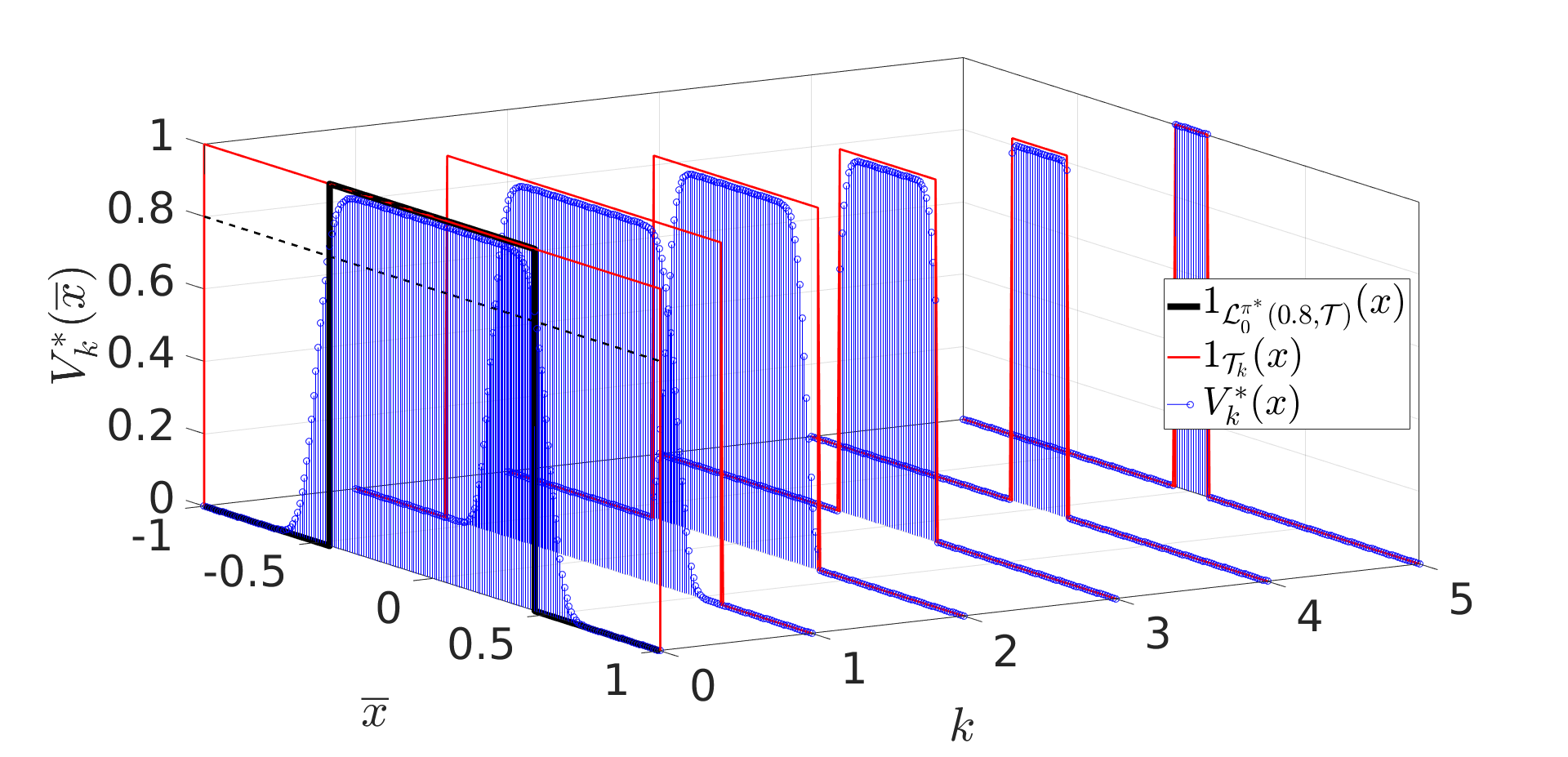
Figure 2: Dynamic programming (8) applied to example (11). We show the evolution of $V_{k}^{\ast}(x)$ and the construction of the stochastic reach set $\mathcal{L}^{\pi^{\ast}}_{0}(\alpha,\mathscr{T})$ for $\alpha=0.8$.

Illustrative example: Consider the one-dimensional system,

$$\boldsymbol{x}_{k+1} =\boldsymbol{x}_{k}+u_{k}+\boldsymbol{w}_{k}$$ (11)

with input $u_{k}\in[-0.1,0.1]$, and disturbance $\boldsymbol{w}_{k}\sim\mathcal{N}(0,0.001)$. Figure 2 shows the dynamic programming solution (8) for the target tube $\mathscr{T}={\{[-\ell^{k},\ell^{k}]\}}_{k=0}^{N}$ with $\ell=0.6$ and time horizon $N=5$. As prescribed by (8a), we set $V_{5}^{\ast}(x)=1_{\mathcal{T}_{5}}(x)$, and we compute $V_{k}^{\ast}(\cdot)$ using the backward recursion (8b) over a grid of $\{-1,-0.99,\ldots,0.99,1\}$. The $0.8$-level stochastic reach set is given by the superlevel set of $V_{0}^{\ast}(\cdot)$ at $0.8$. As expected, the states near the boundary of the target sets become increasingly unsafe as we go backward in time.

2.4 Problem formulation

Table 1: Sufficient conditions for various properties of $V_{k}^{\ast}(\cdot)$ and $\mathcal{L}^{\pi^{\ast}}(\cdot)$. See [1, Thm. 2] for Lipschitz continuity of $V_{k}^{\ast}(\cdot)$.

Property for $k\in\mathbb{N}_{[0,N]}$ $f_{k}$ over $\mathcal{X}\times\mathcal{U}\times\mathcal{W}$ $\mathcal{X}$ (Borel) $\mathcal{U}$ (Compact) $\mathcal{T}_{k}$ (Borel) $Q_{k}$ (Borel-measurable) Result $V_{k}^{\ast}(\cdot)$ over $\mathcal{X}$ $\mathcal{L}^{\pi^{\ast}}_{k}(\alpha,\mathscr{T})$ Measurability Exists $\forall\alpha\in[0,1]$ Measurable - - - Input-continuous Prop. 6a Piecewise continuity Continuous Prop. 6b Upper semi-continuity Closed $\forall\alpha\in[0,1]$ Continuous Closed - Closed - Prop. 7a Compact $\forall\alpha\in(0,1]$ Compact Prop. 7b Log-concavity Convex $\forall\alpha\in[0,1]$ Linear (1) $\mathbb{R}^{n}$ Convex Convex Input-continuous & Log-concave $\psi_{\boldsymbol{w},k}$ Thm. 8 Convex &
closed Log-concave $\psi_{\boldsymbol{w},k}$ Convex & compact $\forall\alpha\in(0,1]$ Linear (1) $\mathbb{R}^{n}$ Convex Convex &
compact Log-concave $\psi_{\boldsymbol{w},k}$ Prop. 10

Figure 3: Various assumptions introduced in Section 3, and the resulting set properties (italicized) of $\mathcal{L}^{\pi^{\ast}}_{k}(\alpha,\mathscr{T})$.

We propose grid-free and tractable algorithms to underapproximate $\mathcal{L}^{\pi^{\ast}}_{0}(\alpha,\mathscr{T})$ based on its set-theoretic properties, in lieu of a grid-based implementation of (8).

Problem 1.

Provide sufficient conditions under which $V_{k}^{\ast}(\cdot)$ is log-concave and the $\alpha$-superlevel set of $V_{k}^{\ast}(\cdot)$, $\mathcal{L}^{\pi^{\ast}}_{k}(\alpha,\mathscr{T})$, is convex for every $k\in\mathbb{N}_{[0,N]}$ and $\alpha\in[0,1]$.

We seek conditions under which the stochastic reachability problem is well-posed, and the stochastic reach set $\mathcal{L}^{\pi^{\ast}}_{k}(\alpha,\mathscr{T})$ is closed, bounded, and compact. Convexity and compactness together enable tight polytopic representations of $\mathcal{L}^{\pi^{\ast}}_{k}(\alpha,\mathscr{T})$. We also seek to exploit these set properties to obtain an underapproximative, grid-free interpolation scheme for real-time computation.

Problem 2.

For any $\beta\in[\alpha_{1},\alpha_{2}]$ such that $0<\alpha_{1}<\alpha_{2}\leq 1$, construct an underapproximative interpolation of $\mathcal{L}^{\pi^{\ast}}_{k}(\beta,\mathscr{T})$ using $\mathcal{L}^{\pi^{\ast}}_{k}(\alpha_{1},\mathscr{T})$ and $\mathcal{L}^{\pi^{\ast}}_{k}(\alpha_{2},\mathscr{T})$ for any $k\in\mathbb{N}_{[0,N]}$.

Problem 3.

Construct a scalable, grid-free, and anytime algorithm to compute an open-loop controller-based polytopic underapproximation to $\mathcal{L}^{\pi^{\ast}}_{k}(\alpha,\mathscr{T}),\ \forall k\in\mathbb{N}_{[0,N]},\ \forall\alpha\in(0,1]$.

3 Stochastic reachability: Properties of (6) & (7)

The relationship between various assumptions introduced in this section is shown in Figure 3, and the set properties are summarized in Table 1.

3.1 Existence, continuity, and compactness

We first adapt results from stochastic optimal control to obtain sufficient conditions under which the stochastic reach set exists, and is closed, bounded, and compact. For the nonlinear stochastic system (3) (and thereby the linear system (1)), these sufficient conditions guarantee the well-posedness of the stochastic reachability problem of a target tube (6). The proofs of Propositions 4, 6, and 7 follow from (9), the measurable selection theorem [23, Thm. 2] [7, Sec. 8.3], and properties of u.s.c. functions, respectively (see Appendix A.1–A.4 for the proofs).

Proposition 4 (Bounded).

Let $\mathcal{L}^{\pi^{\ast}}_{k}(\alpha,\mathscr{T})$ exist for some $k\in\mathbb{N}_{[0,N]}$ and $\alpha\in(0,1]$. Then, $\mathcal{L}^{\pi^{\ast}}_{k}(\alpha,\mathscr{T})\subseteq\mathcal{T}_{k}$, and bounded $\mathcal{T}_{k}$ implies bounded $\mathcal{L}^{\pi^{\ast}}_{k}(\alpha,\mathscr{T})$.

Definition 5 (Continuity of stochastic kernels).

[7, Defn. 7.12] A stochastic kernel $Q(\cdot|\overline{x},\overline{u})$ is said to be:

1. input-continuous, if $\int_{\mathcal{X}}h(\overline{y})Q(d\overline{y}|\overline{x},\overline{u})$ is continuous over $\mathcal{U}$ for each $\overline{x}\in\mathcal{X}$ for any bounded and Borel-measurable function $h:\mathcal{X}\rightarrow\mathbb{R}$.

2. continuous, if $\int_{\mathcal{X}}h(\overline{y})Q(d\overline{y}|\overline{x},\overline{u})$ is continuous over $\mathcal{X}\times\mathcal{U}$ for any bounded and Borel-measurable function $h:\mathcal{X}\rightarrow\mathbb{R}$.

From Definition 5, every continuous stochastic kernel is also input-continuous.

Proposition 6 (Existence).

Consider (6) where $f_{k}(\cdot),\ \forall k\in\mathbb{N}_{[0,N-1]}$ is Borel-measurable over $\mathcal{X}\times\mathcal{U}\times\mathcal{W}$, $\mathcal{U}$ is compact, and $\mathscr{T}={\{\mathcal{T}_{k}\}}_{k=0}^{N}$ such that $\mathcal{T}_{k}\subseteq\mathcal{X},\ \forall k\in\mathbb{N}_{[0,N]}$ are Borel. The following statements are true for every $k\in\mathbb{N}_{[0,N]}$ and $\alpha\in[0,1]$:

1. if $Q_{k}$ is input-continuous for every $k\in\mathbb{N}_{[0,N]}$, then $\pi^{\ast}$ and $\mathcal{L}^{\pi^{\ast}}_{k}(\alpha,\mathscr{T})$ exist, and $V_{k}^{\ast}(\cdot)$ is Borel-measurable.

2. if $Q_{k}$ is continuous for every $k\in\mathbb{N}_{[0,N]}$, then $V_{k}^{\ast}(\cdot)$ is additionally piecewise-continuous over $\mathcal{X}$ in the sense that $V_{k}^{\ast}(\cdot)$ is continuous over the relative interior and the complement of $\mathcal{T}_{k}$.

Proposition 7 (Closed/compact).

Consider (6) where $f_{k}(\cdot),\ \forall k\in\mathbb{N}_{[0,N-1]}$ is continuous over $\mathcal{X}\times\mathcal{U}\times\mathcal{W}$, $\mathcal{X}$ is closed, $\mathcal{U}$ is compact, and $\mathscr{T}={\{\mathcal{T}_{k}\}}_{k=0}^{N}$ such that $\mathcal{T}_{k}\subseteq\mathcal{X},\ \forall k\in\mathbb{N}_{[0,N]}$ are closed. The following statements are true for every $k\in\mathbb{N}_{[0,N]}$ and $\alpha\in[0,1]$:

1. $\pi^{\ast}$ and $\mathcal{L}^{\pi^{\ast}}_{k}(\alpha,\mathscr{T})$ exist, $V_{k}^{\ast}(\cdot)$ is u.s.c. over $\mathcal{X}$, and $\mathcal{L}^{\pi^{\ast}}_{k}(\alpha,\mathscr{T})$ is closed.

2. additionally, if $\mathcal{T}_{k}$ is bounded for some $k\in\mathbb{N}_{[0,N]}$, then $\mathcal{L}^{\pi^{\ast}}_{k}(\alpha,\mathscr{T})$ is compact.

The key difference between assumptions in Proposition 6 and 7 is the replacement of continuity requirements on $Q_{k}$, with stricter requirements on $f_{k}(\cdot)$, $\mathcal{X}$, and $\mathscr{T}{}$. These assumptions do not subsume each other in general, as illustrated in Figure 3.

3.2 Convexity and compactness: Polytopic representation of $\mathcal{L}^{\pi^{\ast}}_{k}(\alpha,\mathscr{T})$

An underapproximative polytope of a closed and convex set is the convex hull of a collection of points within the set [8, Sec. 2.1.4]. Using compactness, this underapproximation can be made tight by identifying the extreme points in the set [45, Thm 2.6.16]. Recall that extreme points of a set are points that cannot be expressed as a convex combination of any two distinct points in the set [45, Ch. 2]. The key benefit of demonstrating convexity of stochastic reach sets is that it enables a grid-free characterization.

Theorem 8 (Convex).

Consider (6) where the system is linear (1), $\mathcal{X}=\mathbb{R}^{n}$, $\mathcal{U}$ is convex and compact, $\mathscr{T}={\{\mathcal{T}_{k}\}}_{k=0}^{N}$ such that $\mathcal{T}_{k}\subseteq\mathcal{X},\ \forall k\in\mathbb{N}_{[0,N]}$ are convex, and $\psi_{\boldsymbol{w},k},\ \forall k\in\mathbb{N}_{[0,N]}$ is a log-concave probability density function. Further, let $Q_{k},\ \forall k\in\mathbb{N}_{[0,N-1]}$ be input-continuous, or the set $\mathcal{T}_{k},\ \forall k\in\mathbb{N}_{[0,N]}$ be closed. Then, $V_{k}^{\ast}(\cdot)$ is log-concave over $\mathcal{X}$ and $\mathcal{L}^{\pi^{\ast}}_{k}(\alpha,\mathscr{T})$ is convex, for every $k\in\mathbb{N}_{[0,N]}$ and $\alpha\in[0,1]$.

Proof: The hypothesis of Theorem 8 ensures that (6) is well-posed and an optimal Markov policy exists by Propositions 6 or 7.

Since $\mathcal{T}_{k}$ are convex, the indicator functions $1_{\mathcal{T}_{k}}(\cdot),\ \forall k\in\mathbb{N}_{[0,N]}$ are log-concave over $\mathcal{X}$. Hence, $V_{N}^{\ast}(\cdot)$ is log-concave over $\mathcal{X}$ by (8a). Next, we will show that $\int_{\mathcal{X}}V_{k+1}^{\ast}(\overline{y})Q_{k}(d\overline{y}|\overline{x},\overline{u})$ is log-concave over $\mathcal{X}\times\mathcal{U}$ for every $k\in\mathbb{N}_{[0,N-1]}$, from which the log-concavity of $V_{k}^{\ast}(\cdot)$ will follow. By (2), for every $k\in\mathbb{N}_{[0,N-1]}$,

$$\int_{\mathcal{X}}V_{k+1}(\overline{y})Q_{k}(d\overline{y}|\overline{x},\overline{u}) =\int_{\mathcal{X}}V_{k+1}(A_{k}\overline{x}+B_{k}\overline{u}+\overline{w})\psi_{\boldsymbol{w},k}(\overline{w})d\overline{w}.$$ (12)

Our proof is by induction. Consider the base case $k=N-1$. To show log-concavity of $\int_{\mathcal{X}}V_{N}(\overline{y})Q_{N-1}(d\overline{y}|\overline{x},\overline{u})$, first recall that compositions of log-concave functions with affine functions preserve log-concavity [8, Sec. 3.2.2]. Hence, $V_{N}(A_{N-1}\overline{x}_{N-1}+B\overline{u}_{N-1}+\overline{w}_{N-1})$ is log-concave over $\mathcal{X}\times\mathcal{U}\times\mathcal{W}$. The proof for log-concavity of $\int_{\mathcal{X}}V_{N}^{\ast}(\overline{y})Q_{N-1}(d\overline{y}|\overline{x},\overline{u})$ is complete with the observation that multiplication and partial integration preserve log-concavity [8, Sec. 3.5.2]. The proof of log-concavity of $V_{N-1}(\cdot)$ follows from the convexity of $\mathcal{U}$ and the fact that log-concavity is preserved under partial supremum over convex sets and multiplication [8, Secs. 3.2.5 and 3.5.2].

For the case $k=t$ with $t\in\mathbb{N}_{[0,N-2]}$, assume for induction that $V_{t+1}^{\ast}(\cdot)$ is log-concave over $\mathcal{X}$. The proofs for the log-concavity of $\int_{\mathcal{X}}V_{t+1}^{\ast}(\overline{y})Q_{t}(d\overline{y}|\overline{x},\overline{u})$ and $V_{t}^{\ast}(\cdot)$ follow by the same arguments as above.

For every $k\in\mathbb{N}_{[0,N]}$, the log-concavity (and thereby, quasiconcavity) of $V_{k}^{\ast}(\cdot)$ implies that the set $\mathcal{L}^{\pi^{\ast}}_{k}(\alpha,\mathscr{T})$ is convex for $\alpha\in[0,1]$.   

Recall that the probability density $\psi_{\boldsymbol{w},k}$ is log-concave if and only if $\boldsymbol{w}_{k}$ has a log-concave probability measure and full-dimensional support [14, Thm. 2.8]. Further, input-continuity of $Q_{k}$ in (2) is guaranteed if $\psi_{\boldsymbol{w},k}$ is a continuous function [7, Sec. 8.3].

Assumption 9.

The system model is linear (1), $\mathcal{X}=\mathbb{R}^{n}$, $\mathcal{U}$ is convex and compact, and $\mathscr{T}={\{\mathcal{T}_{k}\}}_{k=0}^{N}$ such that $\mathcal{T}_{k}\subseteq\mathcal{X}$ are convex and compact $\forall k\in\mathbb{N}_{[0,N]}$, and $\psi_{\boldsymbol{w},k}$ is a log-concave probability density function.

Proposition 10 (Convex and compact).

Under Assumption 9, $\mathcal{L}^{\pi^{\ast}}_{k}(\alpha,\mathscr{T})$ are convex and compact, for every $k\in\mathbb{N}_{[0,N]}$ and $\alpha\in(0,1]$.

Proof: By Proposition 7 and Theorem 8.   

Assumption 9 combines the assumptions in Theorem 8 and Proposition 7b. Theorem 8 and Proposition 10 solve Problem 1. Proposition 10 admits a tight polytopic representation of $\mathcal{L}^{\pi^{\ast}}_{k}(\alpha,\mathscr{T})$ for every $k\in\mathbb{N}_{[0,N]}$ and $\alpha\in(0,1]$. We lose the guarantee of boundedness, and thereby compactness, for $\alpha=0$ (Proposition 4).

3.3 Underapproximative interpolation

We now consider Problem 2. Given the stochastic reach sets at two different thresholds $\alpha_{1},\alpha_{2}\in(0,1]$, we wish to construct an underapproximative interpolation of the stochastic reach set at a desired threshold $\beta\in[\alpha_{1},\alpha_{2}]$.

Theorem 11 (Interpolation via Minkowski sum).

Let Assumption 9 hold, and let $k\in\mathbb{N}_{[0,N]}$ and $\alpha_{1},\alpha_{2}\in(0,1],\ \alpha_{1}<\alpha_{2}$. Then, for any $\beta\in[\alpha_{1},\alpha_{2}]$,

$$\gamma\mathcal{L}^{\pi^{\ast}}_{k}(\alpha_{1},\mathscr{T})\oplus(1-\gamma)\mathcal{L}^{\pi^{\ast}}_{k}(\alpha_{2},\mathscr{T})\subseteq\mathcal{L}^{\pi^{\ast}}_{k}(\beta,\mathscr{T}),$$ (13)

where

$$\gamma =\frac{\log(\alpha_{2})-\log(\beta)}{\log(\alpha_{2})-\log(\alpha_{1})}\in[0,1].$$ (14)

Proof: For any $k\in\mathbb{N}_{[0,N]}$ and $\gamma$ in (14), consider some $\overline{y}\in\gamma\mathcal{L}^{\pi^{\ast}}_{k}(\alpha_{1},\mathscr{T})\oplus(1-\gamma)\mathcal{L}^{\pi^{\ast}}_{k}(\alpha_{2},\mathscr{T})$. Specifically, there exists $\overline{y}_{1}\in\mathcal{L}^{\pi^{\ast}}_{k}(\alpha_{1},\mathscr{T})$ and $\overline{y}_{2}\in\mathcal{L}^{\pi^{\ast}}_{k}(\alpha_{2},\mathscr{T})$ such that $\overline{y}=\gamma\overline{y}_{1}+(1-\gamma)\overline{y}_{2}$, $V_{k}^{\ast}\left(\overline{y}_{1}\right)\geq\alpha_{1}>0$, and $V_{k}^{\ast}\left(\overline{y}_{2}\right)\geq\alpha_{2}>0$. Recall that $z^{\gamma}$ is nondecreasing over positive $z\in\mathbb{R}$. Consequently,

$${\left(V_{k}^{\ast}\left(\overline{y}_{1}\right)\right)}^{\gamma} \geq\alpha_{1}^{\gamma}>0$$ (15a)

$${\left(V_{k}^{\ast}\left(\overline{y}_{2}\right)\right)}^{(1-\gamma)} \geq\alpha_{2}^{(1-\gamma)}>0$$ (15b)

$${\left(V_{k}^{\ast}\left(\overline{y}_{1}\right)\right)}^{\gamma}{\left(V_{k}^{\ast}\left(\overline{y}_{2}\right)\right)}^{(1-\gamma)} \geq\alpha_{1}^{\gamma}\alpha_{2}^{(1-\gamma)}.$$ (15c)

By the definition of $\gamma$ in (14), $\alpha_{1}^{\gamma}\alpha_{2}^{(1-\gamma)}=\beta$. By log-concavity of $V_{k}^{\ast}(\cdot)$ (Theorem 8) and (15), we have $V_{k}^{\ast}\left(\overline{y}\right)\geq{\left(V_{k}^{\ast}\left(\overline{y}_{1}\right)\right)}^{\gamma}{\left(V_{k}^{\ast}\left(\overline{y}_{2}\right)\right)}^{(1-\gamma)}\geq\beta$. Thus, $\overline{y}\in\mathcal{L}^{\pi^{\ast}}_{k}(\beta,\mathscr{T})$, which completes the proof.   

Corollary 12.

Let Assumption 9 hold. Given $\alpha_{1},\alpha_{2}\in(0,1]$, let $\alpha_{1}<\alpha_{2}$, $\overline{x}_{1}^{(1)},\ldots,\overline{x}_{1}^{(K_{1})}\in\mathcal{L}^{\pi^{\ast}}_{k}(\alpha_{1},\mathscr{T})$ and $\overline{x}_{2}^{(1)},\ldots,\overline{x}_{2}^{(K_{2})}\in\mathcal{L}^{\pi^{\ast}}_{k}(\alpha_{2},\mathscr{T})$ for some $K_{1},K_{2}\in\mathbb{N},K_{1},K_{2}>0$, and $k\in\mathbb{N}_{[0,N]}$. For any $\beta\in[\alpha_{1},\alpha_{2}]$ and $\gamma$ defined in (14),

$$\underset{i\in\mathbb{N}_{[1,K_{1}]},j\in\mathbb{N}_{[1,K_{2}]}}{\mathrm{conv}}(\gamma\overline{x}_{1}^{(i)}+(1-\gamma)\overline{x}_{2}^{(j)})\subseteq\mathcal{L}^{\pi^{\ast}}_{k}(\beta,\mathscr{T}).$$

Using Theorem 11 and Corollary 12, we can interpolate stochastic reach sets with minimal computational effort. These interpolations also yield convex, underapproximative sets, since Minkowski sums preserve convexity [8, Sec. 2.1].

4 Underapproximative stochastic reachability of a target tube using open-loop controllers

Next, we address Problem 3. We use open-loop controllers to facilitate the computation of an underapproximation of the maximal reach probability (6) and the stochastic reach set (10). We propose a scalable, grid-free, and anytime algorithm to compute an underapproximative polytope. We use a convex chance constraints approach [44, 27] for highly efficient and scalable polytope computation, which also lowers the computation cost associated with the Fourier transform approach [43]. Finally, we use Corollary 12 to propose a tractable, underapproximative, grid-free, and polytopic interpolation to stochastic reach sets.

4.1 Formulation of the optimization problem

An open-loop policy $\rho:\mathcal{X}\rightarrow\mathcal{U}^{N}$ provides a sequence of inputs $\rho(\overline{x}_{0})={[\overline{u}_{0}^{\top}\ \overline{u}_{1}^{\top}\ \cdots\ \overline{u}_{N-1}^{\top}]}^{\top}$ for every initial condition $\overline{x}_{0}$. Note that all actions of this policy are contingent only on the initial state, and not the current state like in a Markov policy $\pi$. The random vector describing the extended state $\boldsymbol{X}$, under the action of $\overline{U}=\rho(\overline{x}_{0})$, lies in the probability space $(\mathcal{X}^{N},\mathscr{B}(\mathcal{X}^{N}),\mathbb{P}_{\boldsymbol{X}}^{\overline{x}_{0},\overline{U}})$. Under $\rho(\cdot)$, the open-loop reach probability is

$$r_{\overline{x}_{0}}^{\rho}(\mathscr{T}) \triangleq 1_{\mathcal{T}_{0}}(\overline{x}_{0})\mathbb{P}_{\boldsymbol{X}}^{\overline{x}_{0},\overline{U}}\left\{\boldsymbol{X}\in\bigtimes_{k=1}^{N}\mathcal{T}_{k}\right\}.$$ (16)

With optimal open-loop controller $\rho^{\ast}$, we define the maximal open-loop reach probability $W_{0}^{\ast}:\mathcal{X}\rightarrow[0,1]$ as

$$W_{0}^{\ast}(\overline{x}_{0}) \triangleq r_{\overline{x}_{0}}^{\rho^{\ast}}(\mathscr{T})=\sup_{\rho(\overline{x}_{0})=\overline{U}\in\mathcal{U}^{N}}r_{\overline{x}_{0}}^{\rho}(\mathscr{T}).$$ (17)

Similarly to (8), we define $W_{k}:\mathcal{X}\times\mathcal{U}^{N-k}\rightarrow[0,1]$ for every $k\in\mathbb{N}_{[0,N-1]}$,

$$W_{k}(\overline{x},\overline{U}_{k:N}) =1_{\mathcal{T}_{k}}(\overline{x})\int_{\mathcal{X}}W_{k+1}(\overline{y},\overline{U}_{k+1:N})Q_{k}(d\overline{y}|\overline{x},\overline{u}_{k})$$ (18a)

$$W_{0}^{\ast}(\overline{x}_{0}) =\sup_{\overline{U}\in\mathcal{U}^{N}}W_{0}(\overline{x}_{0},\overline{U})$$ (18b)

where $W_{N}(\overline{x},\overline{U}_{N:N})=1_{\mathcal{T}_{N}}(\overline{x})$. Here, for every $k\in\mathbb{N}_{[0,N-1]}$, $\overline{U}_{k:N}={[\overline{u}_{k}^{\top}\ \overline{u}_{k+1}^{\top}\ \cdots\ \overline{u}_{N-1}^{\top}]}^{\top}\in\mathcal{U}^{N-k}$ with $\overline{U}_{k:N}$, $\overline{U}_{N-1:N}=\overline{u}_{N-1}$, and $\overline{U}_{0:N}=\overline{U}$. Since $W_{0}(\overline{x}_{0},\overline{U})=r_{\overline{x}_{0}}^{\rho}(\mathscr{T})$ for $\rho(\overline{x}_{0})=\overline{U}$, the optimization problems (17) and (18b) are equivalent with identical objectives and constraints.

Similarly to (7), we define the $\alpha$-superlevel set of $r_{\overline{x}_{0}}^{\rho^{\ast}}(\mathscr{T})$,

$$\mathcal{K}^{\rho^{\ast}}_{0}(\alpha,\mathscr{T}) =\{\overline{x}_{0}\in\mathcal{X}:r_{\overline{x}_{0}}^{\rho^{\ast}}(\mathscr{T})\geq\alpha\}.$$ (19)

Proposition 13.

Let Assumption 9 hold. Then, the following statements are true:

1. $W_{0}^{\ast}(\cdot)$ is well-defined and u.s.c.over $\mathcal{X}$.

2. $W_{0}^{\ast}(\overline{x})\leq V_{0}^{\ast}(\overline{x}),\ \forall\overline{x}\in\mathcal{X}$, and $\mathcal{K}^{\rho^{\ast}}_{0}(\alpha,\mathscr{T})\subseteq\mathcal{L}^{\pi^{\ast}}_{0}(\alpha,\mathscr{T}),\ \forall\alpha\in[0,1]$.

3. (17) is a log-concave optimization problem, $W_{0}(\cdot,\cdot)$ is log-concave over $\mathcal{X}\times\mathcal{U}^{N}$, and $W_{0}^{\ast}(\cdot)$ is log-concave over $\mathcal{X}$.

4. $\mathcal{K}^{\rho^{\ast}}_{0}(\alpha,\mathscr{T}),\ \forall\alpha\in(0,1]$ is convex and compact.

The proof of Proposition 13 is given in Appendix A.5.

4.2 Construction of a polytopic underapproximation of $\mathcal{K}^{\rho^{\ast}}_{0}(\alpha,\mathscr{T})$ under Assumption 9

Given a finite set $\mathcal{D}\subset\mathcal{X}$ consisting of direction vectors $\bar{d}_{i}$, we compute a polytopic underapproximation of $\mathcal{K}^{\rho^{\ast}}_{0}(\alpha,\mathscr{T})$ in three steps (Figure 4):

1. find $\overline{x}_{\mathrm{anchor}}\in\mathcal{T}_{0}$, referred to as the anchor point, such that $W_{0}^{\ast}(\overline{x}_{\mathrm{anchor}})\geq\alpha$; if no such point exists, then $\mathcal{K}^{\rho^{\ast}}_{0}(\alpha,\mathscr{T})=\emptyset$; else, continue to step 2,

2. obtain relative boundary points of the set $\mathcal{K}^{\rho^{\ast}}_{0}(\alpha,\mathscr{T})$ via line searches from $\overline{x}_{\mathrm{anchor}}$ along the directions $\bar{d}_{i}\in\mathcal{D}$, and

3. compute the convex hull of the relative boundary points, i.e., the polytope $\underline{\mathcal{K}^{\rho^{\ast}}_{0}}(\alpha,\mathscr{T},\mathcal{D})$.

By [8, Sec. 2.1.4] and Proposition 13b,

$$\underline{\mathcal{K}^{\rho^{\ast}}_{0}}(\alpha,\mathscr{T},\mathcal{D})\subseteq\mathcal{K}^{\rho^{\ast}}_{0}(\alpha,\mathscr{T})\subseteq\mathcal{L}^{\pi^{\ast}}_{0}(\alpha,\mathscr{T}).$$ (20)

Thus, we can utilize the compactness and convexity of $\mathcal{K}^{\rho^{\ast}}_{0}(\alpha,\mathscr{T})$ (Proposition 13d) to obtain a polytopic underapproximation $\underline{\mathcal{K}^{\rho^{\ast}}_{0}}(\alpha,\mathscr{T},\mathcal{D})$. We have $\underline{\mathcal{K}^{\rho^{\ast}}_{0}}(\alpha,\mathscr{T},\mathcal{D})=\mathcal{K}^{\rho^{\ast}}_{0}(\alpha,\mathscr{T})$ when all of the extreme points of $\mathcal{K}^{\rho^{\ast}}_{0}(\alpha,\mathscr{T})$ are discovered in step 2. This is possible for a polytopic $\mathcal{K}^{\rho^{\ast}}_{0}(\alpha,\mathscr{T})$ [45, Thm. 2.6.16].

Figure 4: Components of Algorithm 1 using $\overline{x}_{\mathrm{anchor}}=\overline{x}_{\mathrm{max}}$. We solve (25) to compute $W_{0}^{\ast}(\overline{x}_{\mathrm{max}})$, and then solve (35) for each $\overline{d}_{i}\in\mathcal{D}$ to compute the vertices of $\underline{\mathcal{K}^{\rho^{\ast}}_{0}}(\alpha,\mathscr{T},\mathcal{D})$. We construct $\underline{\mathcal{K}^{\rho^{\ast}}_{0}}(\alpha,\mathscr{T},\mathcal{D})$ via the convex hull of the vertices.

First, we propose two possible anchor points $\overline{x}_{\mathrm{anchor}}$: 1) $\overline{x}_{\mathrm{max}}$, the maximizer of $W_{0}^{\ast}(\overline{x})$, and 2) $\overline{x}_{c}$, a Chebyshev center-like point. For the former, the point $\overline{x}_{\mathrm{max}}$ can be computed by solving the optimization problem,

$$\begin{array}[]{rl}\underset{\overline{x},\overline{U},\phi}{\mathrm{maximize}}&\phi\\ \mathrm{subject\ to}&\left\{\begin{array}[]{l}\overline{x}\in\mathcal{T}_{0},\ \overline{U}\in\mathcal{U}^{N},\ \phi\in[0,1],\\ W_{0}(\overline{x},\overline{U})\geq\phi\geq\alpha\\ \end{array}\right.\end{array}$$ (25)

Problem (25) is the epigraph form of the optimization problem $\sup_{\overline{x}_{0}\in\mathcal{K}^{\rho^{\ast}}_{0}(\alpha,\mathscr{T})}W_{0}^{\ast}(\overline{x}_{0})$ [8, Eq. 4.11].

For the latter, $\overline{x}_{c}$ can be computed by solving the following optimization problem, motivated by the Chebyshev centering problem [8, Sec. 8.5.1],

$$\begin{array}[]{rl}\underset{\overline{x},\overline{U},R}{\mathrm{maximize}}&R\\ \mathrm{subject\ to}&\left\{\begin{array}[]{l}\{\overline{x}\}\oplus\mathrm{Ball}(\overline{0},R)\subseteq\mathcal{T}_{0}\\ W_{0}(\overline{x},\overline{U})\geq\alpha,\ \overline{U}\in\mathcal{U}^{N},\ R\geq 0\\ \end{array}\right.\end{array}$$ (30)

Problem (30) seeks an anchor point “deep” inside $\mathcal{T}_{0}$, while ensuring $W_{0}(\overline{x},\overline{U})\geq\alpha$ for some $\overline{U}\in\mathcal{U}^{N}$. The centering constraint, $\{\overline{x}\}\oplus\mathrm{Ball}(\overline{0},R)\subseteq\mathcal{T}_{0}$, is equivalently expressed as $\overline{x}+\overline{s}\in\mathcal{T}_{0},\ \forall\overline{s}\in\mathrm{Ball}(\overline{0},R)$. For a polytopic $\mathcal{T}_{0}$, this is a second order-cone (convex) constraint, and can be enforced efficiently [8, Sec. 8.5.1].

Proposition 14.

Under Assumption 9, (25) and (30) are convex optimization problems.

Proof: We know $W_{0}(\overline{x},\overline{U})$ is a quasiconcave function over $\mathcal{X}\times\mathcal{U}$ by Proposition 13c and the fact that log-concave functions are quasiconcave [8, Sec. 3.5]. Therefore, $W_{0}(\overline{x},\overline{U})\geq\phi$ is a convex constraint involving $\overline{x},\overline{U}$, and $\phi$. Hence (25) and (30) are convex, since all other constraints and their respective objectives are convex.   

For non-empty sets $\mathcal{T}_{k}$ and $\mathcal{U}$, the optimization problems (25) or (30) are infeasible if and only if $\mathcal{K}^{\rho^{\ast}}_{0}(\alpha,\mathscr{T})$ is empty. However, $\mathcal{K}^{\rho^{\ast}}_{0}(\alpha,\mathscr{T})$ being empty does not imply $\mathcal{L}^{\pi^{\ast}}_{0}(\alpha,\mathscr{T})$ is empty, due to the underapproximative nature of our approach.

Next, we compute the relative boundary points of $\mathcal{K}^{\rho^{\ast}}_{0}(\alpha,\mathscr{T})$ by solving (35) for each $i\in\mathbb{N}_{[1,|\mathcal{D}|]}$,

$$\begin{array}[]{rl}\underset{\theta_{i},\overline{U}_{i}}{\mathrm{maximize}}&\theta_{i}\\ \mathrm{subject\ to}&\left\{\begin{array}[]{l}\overline{U}_{i}\in\mathcal{U}^{N},\quad\theta_{i}\in\mathbb{R},\quad\theta_{i}\geq 0\\ W_{0}(\overline{x}_{\mathrm{anchor}}+\theta_{i}\bar{d}_{i},\overline{U}_{i})\geq\alpha\\ \end{array}\right.\end{array}.$$ (35)

Problem (35) is a line search problem [8, Sec. 9.3]. By Proposition 14, (35) is a convex optimization problem under Assumption 9.

Denote the optimal solution of (35) as $\theta^{\ast}_{i}$ and $\overline{U}^{\ast}_{i}$. By construction, $W_{0}(\overline{x}_{\mathrm{anchor}}+\theta_{i}^{\ast}\bar{d}_{i},\overline{U}_{i}^{\ast})=\alpha$, and for any $\epsilon>0$, $W_{0}(\overline{x}_{\mathrm{anchor}}+(\theta_{i}^{\ast}+\epsilon)\bar{d}_{i},\overline{U}_{i}^{\ast})<\alpha$. Hence, $\overline{x}_{\mathrm{anchor}}+\theta_{i}^{\ast}\bar{d}_{i}$ is a relative boundary point of $\mathcal{K}^{\rho^{\ast}}_{0}(\alpha,\mathscr{T})$, and an open-loop controller that ensures $W_{0}(\overline{x}_{\mathrm{anchor}}+\theta_{i}^{\ast}\bar{d}_{i},\overline{U}_{i}^{\ast})\geq\alpha$ is $\rho^{\ast}(\overline{x}_{\mathrm{anchor}}+\theta_{i}^{\ast}\bar{d}_{i})=\overline{U}_{i}^{\ast}$. Note that $W_{0}(\overline{x}_{\mathrm{anchor}}+\theta_{i}^{\ast}\bar{d}_{i},\overline{U}_{i}^{\ast})$ is not necessarily equal to the maximal open-loop reach probability $W_{0}^{\ast}(\overline{x}_{\mathrm{anchor}}+\theta_{i}^{\ast}\bar{d}_{i})$, since we have only required that $W_{0}(\overline{x}_{\mathrm{anchor}}+\theta_{i}^{\ast}\bar{d}_{i},\overline{U}_{i}^{\ast})\geq\alpha$ in (35).

We construct the polytope $\underline{\mathcal{K}^{\rho^{\ast}}_{0}}(\alpha,\mathscr{T},\mathcal{D})$ via the convex hull of the computed relative boundary points $\overline{x}_{\mathrm{anchor}}+\theta_{i}^{\ast}\bar{d}_{i},\ \forall i\in\mathbb{N}_{[1,|\mathcal{D}|]}$. We have $\underline{\mathcal{K}^{\rho^{\ast}}_{0}}(\alpha,\mathscr{T},\mathcal{D})\subseteq\mathcal{K}^{\rho^{\ast}}_{0}(\alpha,\mathscr{T})$, since $\mathcal{K}^{\rho^{\ast}}_{0}(\alpha,\mathscr{T})$ is convex and compact, and the vertices of $\underline{\mathcal{K}^{\rho^{\ast}}_{0}}(\alpha,\mathscr{T},\mathcal{D})$ lie in $\partial\mathcal{K}^{\rho^{\ast}}_{0}(\alpha,\mathscr{T})$ [8, Sec. 2.1.4].

We summarize our approach in Algorithm 1, which solves Problem 3.

Algorithm 1 Compute polytope $\underline{\mathcal{K}^{\rho^{\ast}}_{0}}(\alpha,\mathscr{T},\mathcal{D})$, an underapproximation of the stochastic reach set $\mathcal{L}^{\pi^{\ast}}_{0}(\alpha,\mathscr{T})$

1:System (1), target tube $\mathscr{T}$, probability threshold $\alpha$, set of direction vectors $\mathcal{D}$

2:$\underline{\mathcal{K}^{\rho^{\ast}}_{0}}(\alpha,\mathscr{T},\mathcal{D})\subseteq\mathcal{K}^{\rho^{\ast}}_{0}(\alpha,\mathscr{T})\subseteq\mathcal{L}^{\pi^{\ast}}_{0}(\alpha,\mathscr{T})$

3:Solve (25) or (30) to compute $\overline{x}_{\mathrm{anchor}}$

4:if (25) or (30) is infeasible then

5:     $\underline{\mathcal{K}^{\rho^{\ast}}_{0}}(\alpha,\mathscr{T},\mathcal{D})\leftarrow\emptyset$

6:else

7:     for $\bar{d}_{i}\in\mathcal{D}$ do

8:         Solve (35) to compute a relative boundary point $\overline{x}_{\mathrm{anchor}}+\theta_{i}^{\ast}\bar{d}_{i}$ and an open-loop controller $\rho^{\ast}(\overline{x}_{\mathrm{anchor}}+\theta_{i}^{\ast}\bar{d}_{i})$

9:     end for

10:     $\underline{\mathcal{K}^{\rho^{\ast}}_{0}}(\alpha,\mathscr{T},\mathcal{D})\leftarrow\underset{i\in\mathbb{N}_{[1,|\mathcal{D}|]}}{\mathrm{conv}}(\overline{x}_{\mathrm{anchor}}+\theta_{i}^{\ast}\bar{d}_{i})$

11:end if

4.3 Implementation of Algorithm 1

Algorithm 1 is an anytime, parallelizable algorithm. The anytime property follows from the observation that the convex hull of the solutions of (35) for an arbitrary subset of $\mathcal{D}$ also yields a valid underapproximation, permitting premature termination. The parallelizability of Algorithm 1 is due to the fact that the computations along each of the directions $\bar{d}_{i}$ are independent.

Computing $\overline{x}_{\mathrm{anchor}}$ is a significant part of Algorithm 1. Using $\overline{x}_{c}$ may be advantageous because directions typically yield non-trivial relative boundary points, however, it is possible that $\overline{x}_{c}$ is a relative boundary point of $\underline{\mathcal{K}^{\rho^{\ast}}_{0}}(\alpha,\mathscr{T},\mathcal{D})$ (e.g., Figure 10, bottom). Additionally, solving (30) requires more computational effort due to the second-order cone constraint. However, the “best” choice may be problem-specific. Indeed, using multiple anchor points could be advantageous, as the convex hull of the union of the resulting underapproximations could yield a significantly larger underapproximative set. The implementation of Algorithm 1 in SReachTools provides all three of these options. SReachTools is an open-source MATLAB toolbox for stochastic reachability [41]. SReachTools has participated in several repeatability-evaluations including the recent ARCH initiative for stochastic modeling and verification [2].

Denoting the computation times to solve for $\overline{x}_{\mathrm{anchor}}$ ((25) or (30)) and (35) as $t_{\mathrm{anchor}}$ and $t_{\mathrm{line}}$, respectively, the computation time for Algorithm 1 is $\mathcal{O}(t_{\mathrm{anchor}}+t_{\mathrm{line}}|\mathcal{D}|)$. Since (25), (30), and (35) are convex problems, globally optimal solutions are assured with (potentially) low $t_{\mathrm{anchor}}$ and $t_{\mathrm{line}}$. However, the joint chance constraint $W_{0}(\overline{x},\overline{U})\geq\phi$ is not solver-friendly, since we do not have a closed-form expression for $W_{0}(\overline{x},\overline{U})$, or an exact reformulation into a conic constraint. In Section 4.5 (see Table 2), we discuss computationally efficient methods to enforce this constraint under additional assumptions.

The memory requirements of Algorithm 1 grow linearly with $|\mathcal{D}|$ and are independent of the system dimension. The choice of $\mathcal{D}$ influences the quality (in terms of volume) of underapproximation provided by Algorithm 1. In contrast, dynamic programming requires an exponential number of grid points in memory, leading to the curse of dimensionality [1]. Algorithm 1 is grid-free and recursion-free, and it scales favorably with the system dimension, as compared to dynamic programming.

Open-loop controller synthesis: As a side product of Algorithm 1, solving (35) provides valid open-loop controllers for the vertices of $\underline{\mathcal{K}^{\rho^{\ast}}_{0}}(\alpha,\mathscr{T},\mathcal{D})$ that satisfy (19). Denoting the vertices of $\underline{\mathcal{K}^{\rho^{\ast}}_{0}}(\alpha,\mathscr{T},\mathcal{D})$ as $\{\overline{v}_{i}\}_{i=1}^{|\mathcal{D}|}$, any initial state of interest $\overline{x}_{0}\in\underline{\mathcal{K}^{\rho^{\ast}}_{0}}(\alpha,\mathscr{T},\mathcal{D})$ can be expressed as the convex combination of the vertices, $\overline{x}_{0}=\sum_{i=1}^{|\mathcal{D}|}\gamma_{i}\overline{v}_{i}$ for some $\gamma_{i}\in[0,1]$ and $\sum_{i=1}^{|\mathcal{D}|}\gamma_{i}=1$ [45, Ch. 2]. Consequently, $\sum_{i=1}^{|\mathcal{D}|}\gamma_{i}\overline{U}_{i}^{\ast}$ is a good initial guess to solve (17) at $\overline{x}_{0}$.

4.4 Tractable underapproximative interpolation

In scenarios where stochastic reach sets $\underline{\mathcal{K}^{\rho^{\ast}}_{0}}(\cdot,\mathscr{T},\mathcal{D})$ must be computed at multiple probability thresholds, we propose a computationally efficient algorithm that combines Algorithm 1 and Corollary 12. Specifically, we utilize Algorithm 1 to compute the underapproximations at two specific probability thresholds $\alpha_{1},\alpha_{2}\in(0,1]$ with $\alpha_{1}<\alpha_{2}$, and then utilize Corollary 12 to obtain underapproximative interpolations for all probability thresholds $\beta\in[\alpha_{1},\alpha_{2}]$. We summarize this approach in Algorithm 2. Algorithm 2 enables real-time stochastic reachability by computing a few stochastic reach sets offline and then interpolating them online.

Algorithm 2 Underapproximative interpolation

1:Probability thresholds $\alpha_{1},\alpha_{2}\in(0,1]$ with $\alpha_{1}<\alpha_{2}$, sets of direction vectors $\mathcal{D}_{1}$ and $\mathcal{D}_{2}$, probability thresholds of interest $\beta_{i}\in[\alpha_{1},\alpha_{2}]$ for $i\in\mathbb{N}_{[1,N_{\beta}]}$

2:Polytope $\mathcal{S}_{i}\subseteq\mathcal{L}^{\pi^{\ast}}_{0}(\beta_{i},\mathscr{T})$ for $i\in\mathbb{N}_{[1,N_{\beta}]}$

3:Offline (independent of $\beta_{(\cdot)}$):

4:Compute sets $\underline{\mathcal{K}^{\rho^{\ast}}_{0}}(\alpha_{1},\mathscr{T},\mathcal{D}_{1})$ and $\underline{\mathcal{K}^{\rho^{\ast}}_{0}}(\alpha_{2},\mathscr{T},\mathcal{D}_{2})$ using Algorithm 1

5:Online (depends on $\beta_{(\cdot)}$):

1:for each $\beta_{i}$ do

2:     $\gamma_{i}=\frac{\log(\alpha_{2})-\log(\beta_{i})}{\log(\alpha_{2})-\log(\alpha_{1})}\in[0,1]$

3:     $\mathcal{S}_{i}\leftarrow\gamma_{i}\underline{\mathcal{K}^{\rho^{\ast}}_{0}}(\alpha_{1},\mathscr{T},\mathcal{D}_{1})\oplus(1-\gamma_{i})\underline{\mathcal{K}^{\rho^{\ast}}_{0}}(\alpha_{2},\mathscr{T},\mathcal{D}_{2})$

4:end for

4.5 Gaussian linear time-varying systems with polytopic input space and polytopic target tube

Assumption 15.

Presume Assumption 9, polytopic $\mathcal{U}$ and $\mathcal{T}_{k}$ for every $k\in\mathbb{N}_{[0,N]}$, and Gaussian $\boldsymbol{w}_{k}\sim\mathcal{N}(\overline{\mu}_{\boldsymbol{w},k},C_{\boldsymbol{w},k})$, $\overline{\mu}_{\boldsymbol{w},k}\in\mathbb{R}^{n},C_{\boldsymbol{w},k}\in\mathbb{R}^{n\times n}$.

The concatenated disturbance random vector is $\boldsymbol{W}\sim\mathcal{N}(\overline{\mu}_{\boldsymbol{W}},C_{\boldsymbol{W}})$, where $\overline{\mu}_{\boldsymbol{W}}={[\overline{\mu}_{\boldsymbol{w},0}^{\top}\ \cdots\ \overline{\mu}_{\boldsymbol{w},N-1}^{\top}]}^{\top}\in\mathbb{R}^{nN}$ and $C_{\boldsymbol{W}}=\mathrm{blkdiag}(C_{\boldsymbol{w},0},\ldots,C_{\boldsymbol{w},N-1})\in\mathbb{R}^{nN\times nN}$, with $\mathrm{blkdiag}(\cdot)$ indicating block diagonal matrix construction. Due to the linearity of the system (1), $\boldsymbol{X}$ is also Gaussian [21, Sec. 9.2]. Given an initial state $\overline{x}_{0}\in\mathcal{X}$ and an open-loop vector $\overline{U}\in\mathcal{U}^{N}$,

$$\boldsymbol{X} \sim\mathcal{N}(\overline{\mu}_{\boldsymbol{X}},C_{\boldsymbol{X}}),$$ (36a)

$$\overline{\mu}_{\boldsymbol{X}} =\mathscr{A}\overline{x}_{0}+H\overline{U}+G\overline{\mu}_{\boldsymbol{W}},$$ (36b)

$$C_{\boldsymbol{X}} =GC_{\boldsymbol{W}}G^{\top},$$ (36c)

where $\boldsymbol{X}=\mathscr{A}\overline{x}_{0}+H\overline{U}+G\boldsymbol{W}$. The matrices $\mathscr{A},H,G$ account for how the dynamics (1) influence the mean and the covariance of $\boldsymbol{X}$ (see [36] for details).

Algorithm 1 requires an efficient enforcement of joint chance constraints, $W_{0}(\overline{x},\overline{U})\geq\phi$ in (25), (30), and (35). Under Assumption 15, $W_{0}(\overline{x},\overline{U})$ is the integration of a Gaussian probability density function over a polytope.

Table 2: Enforcing $W_{0}(\overline{x}_{0},\overline{U})\geq\phi$ under Assumption 15.

Approach	Approximation	Solver
Convex chance constraints [27, 31, 44]	Convex restriction via Boole’s inequality	Linear program
Fourier transform [42, 43]	Approximates $W_{0}(\cdot)$ via Genz’s algorithm (quasi-Monte Carlo simulation [18])	Gradient-free optimization solver [26] (patternsearch)

Figure 5: Underapproximative steps taken to compute the polytopic underapproximation $\underline{\mathcal{K}^{\rho^{\ast}}_{0}}(\alpha,\mathscr{T},\mathcal{D})$ of the stochastic reach set $\mathcal{L}^{\pi^{\ast}}_{0}(\alpha,\mathscr{T})$ (Section 4.5) via chance constraints.

Table 2 describes two approaches to approximate $W_{0}(\overline{x},\overline{U})$. We implement convex chance constraints via risk allocation [27, 31, 44]. However, in contrast to solving a series of linear programs [31] or relying on nonlinear solvers [27], we use piecewise affine approximation to obtain a collection of linear constraints that conservatively enforce the constraint $W_{0}(\overline{x},\overline{U})\geq\phi$ at significantly lower computational costs [44]. This ensures that (25) and (35) are linear programs, (30) is a second order-cone program, and enables the use of standard conic solvers [20, 4]. In the Fourier transform approach, we initialize MATLAB’s patternsearch using the solution obtained with the chance constraints implementation. We use anchor points $\overline{x}_{c}$ with convex chance constraints and $\overline{x}_{\mathrm{max}}$ with the Fourier transform approach. Figure 5 summarizes the conservativeness introduced at different stages of the convex chance constraints approach.

5 Numerical results

All computations were performed on a standard laptop with an Intel i7-4600U CPU with 4 cores, 2.1GHz clock rate and 7.5 GB RAM. We used SReachTools [41] in a MATLAB 2018 environment, with MPT3 [22], CVX [20], and MOSEK [4] in the simulations. The code is available online at https://github.com/unm-hscl/abyvinod-SRTT-2020.git.

5.1 Integrator chain: Interpolation & scalability

Consider a chain of integrators,

$$\boldsymbol{x}_{k+1} =\left[{\begin{array}[]{ccccc}1&N_{s}&\frac{N_{s}^{2}}{2}&\cdots&\frac{N_{s}^{n-1}}{(n-1)!}\\ 0&1&N_{s}&\cdots&\\ \vdots&&&\ddots&\vdots\\ 0&0&0&\cdots&1\\ \end{array}}\right]\boldsymbol{x}_{k}+\left[\begin{array}[]{c}\frac{N_{s}^{n}}{n!}\\ \frac{N_{s}^{n-1}}{(n-1)!}\\ \vdots\\ N_{s}\end{array}\right]u_{k}+\boldsymbol{w}_{k}$$ (45)

with state $\boldsymbol{x}_{k}\in\mathbb{R}^{n}$, input $u_{k}\in\mathcal{U}\subset\mathbb{R}$, a Gaussian disturbance $\boldsymbol{w}_{k}\sim\mathcal{N}(\overline{0}_{n},0.01I_{n})$, sampling time $N_{s}=0.1$, and time horizon $N$. Here, $I_{n}$ refers to the $n$-dimensional identity matrix and $\overline{0}_{n}$ is the $n$-dimensional zero vector.

For the double integrator ($n=2$), we consider the stochastic viability problem [1], with $\mathcal{T}_{k}={[-1,1]}^{2}$, $k\in\mathbb{N}_{[0,N]}$ for $N=10$, and $\mathcal{U}=[-0.1,0.1]$. We compute $\underline{\mathcal{K}^{\rho^{\ast}}_{0}}(\alpha,\mathscr{T},\mathcal{D})$ using Algorithm 1 via convex chance constraints (SReachSetCcO in SReachTools) with $|\mathcal{D}|=32$, and compare it to $\mathcal{L}^{\pi^{\ast}}_{0}(\alpha,\mathscr{T})$ from grid-based dynamic programming (SReachDynProg in SReachTools), with grid spacing of 0.05 in the state and input spaces.

Figure 6a shows that Algorithm 1, which computes $\underline{\mathcal{K}^{\rho^{\ast}}_{0}}(\alpha,\mathscr{T},\mathcal{D})$, provides a good underapproximation of the true stochastic reach set $\mathcal{L}^{\pi^{\ast}}_{0}(\alpha,\mathscr{T})$. The advantage of using state-feedback $\pi^{\ast}$ over an open loop controller $\rho^{\ast}$ is seen in the underapproximation “gaps” between the polytopes (Proposition 13b). In Figure 6b, the interpolated polytopic underapproximation (from Corollary 12 and Algorithm 2) provides a good approximation of the true sets $\mathcal{L}^{\pi^{\ast}}_{0}(\beta,\mathscr{T})$ and $\mathcal{K}^{\rho^{\ast}}_{0}(\beta,\mathscr{T})$ at $\beta=0.85$.

To demonstrate scalability, we consider the stochastic reach-avoid problem with a $40$D integrator, with $N=5$, $\mathcal{T}_{k}={[-10,10]}^{40}$ for $k\in\mathbb{N}_{[0,N-1]}$, $\mathcal{T}_{N}={[-8,8]}^{40}$, and $\mathcal{U}=[-1,1]$. Dynamic programming is clearly not feasible for comparison. A $2$D slice of the polytopic underapproximation, at $\overline{x}_{0}={[x_{1}\ x_{2}\ 0\ 0\ \cdots\ 0]}^{\top}\in\mathbb{R}^{40}$, is shown in Figure 6c for $|\mathcal{D}|=8$, computed via Algorithm 1 with convex chance constraints. As shown in Figure 6d, that the underapproximative interpolation obtained from Algorithm 2 appears to be tight; the high ratio ($0.994$) of the volume of interpolated polytopic underapproximation to the volume of $\underline{\mathcal{K}^{\rho^{\ast}}_{0}}(\alpha,\mathscr{T},\mathcal{D})$ confirms this.

Table 3: Computation time (in seconds) for a chain of integrators.

	$n=2$ ($|\mathcal{D}|=32$)			$n=40$ ($|\mathcal{D}|=8$)
$\alpha$	$0.6$	$0.85$	$0.9$	$0.6$	$0.85$	$0.9$
Algorithm 1	$11.86$	$10.12$	$9.80$	$921.29$	$842.29$	$781.78$
Algorithm 2	–	$0.006$	–	–	$0.013$	–
Dyn. prog.	$5.94$			Not possible
Theorem 11	–	$0.035$	–

As expected, Algorithm 1 outperforms dynamic programming in computation time (Table 3). This is a direct consequence of the convexity, compactness, and underapproximative properties established in Section 4. The interpolation scheme provided in Algorithm 2 is faster than Algorithm 1 by three orders of magnitude in $2$D, and by four orders of magnitude in $40$D.

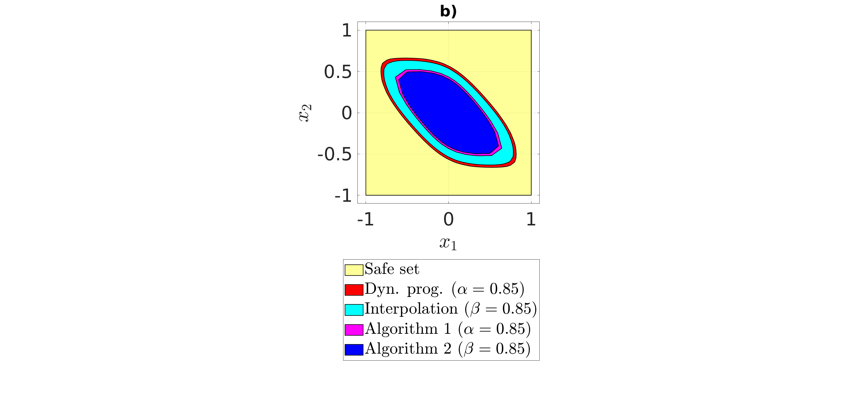
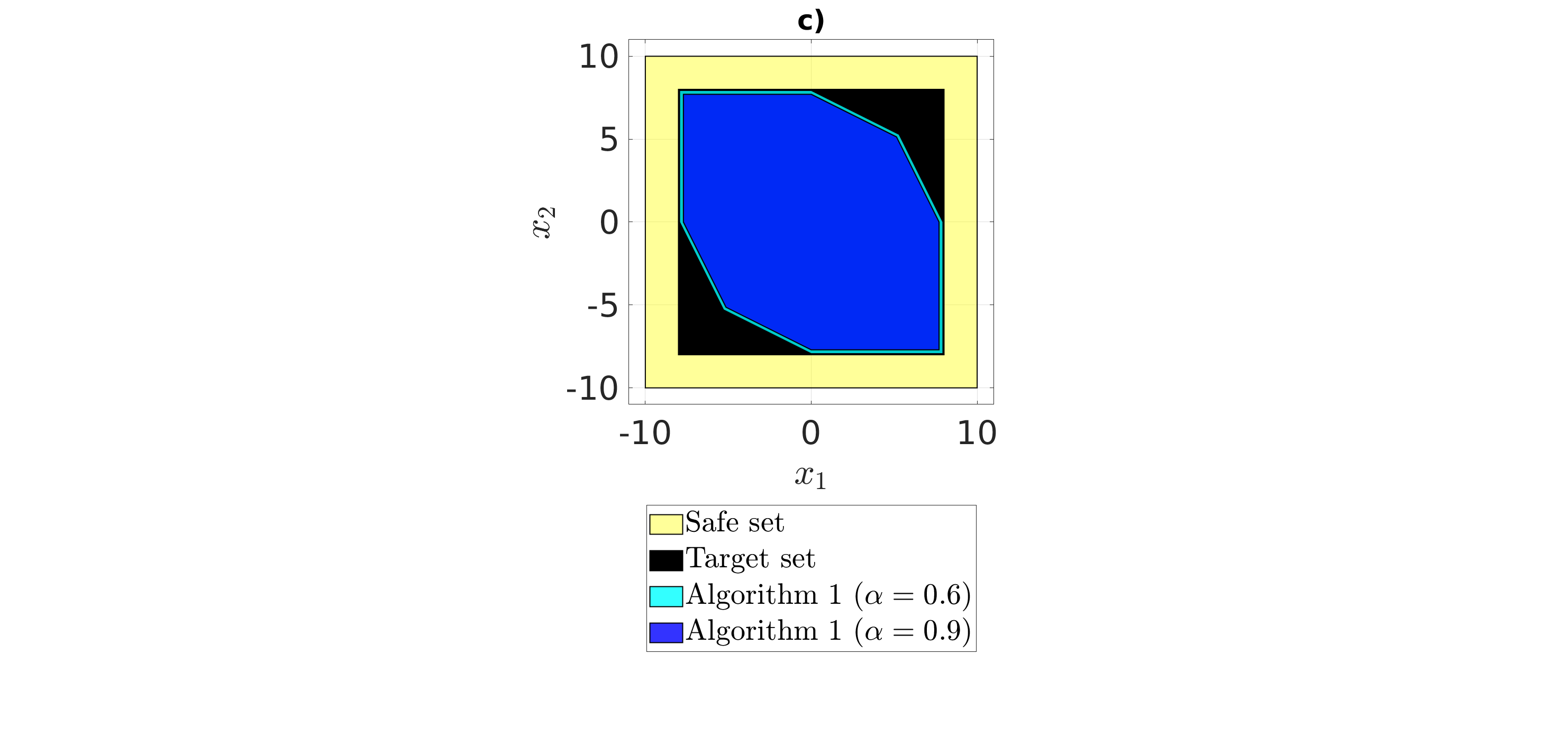
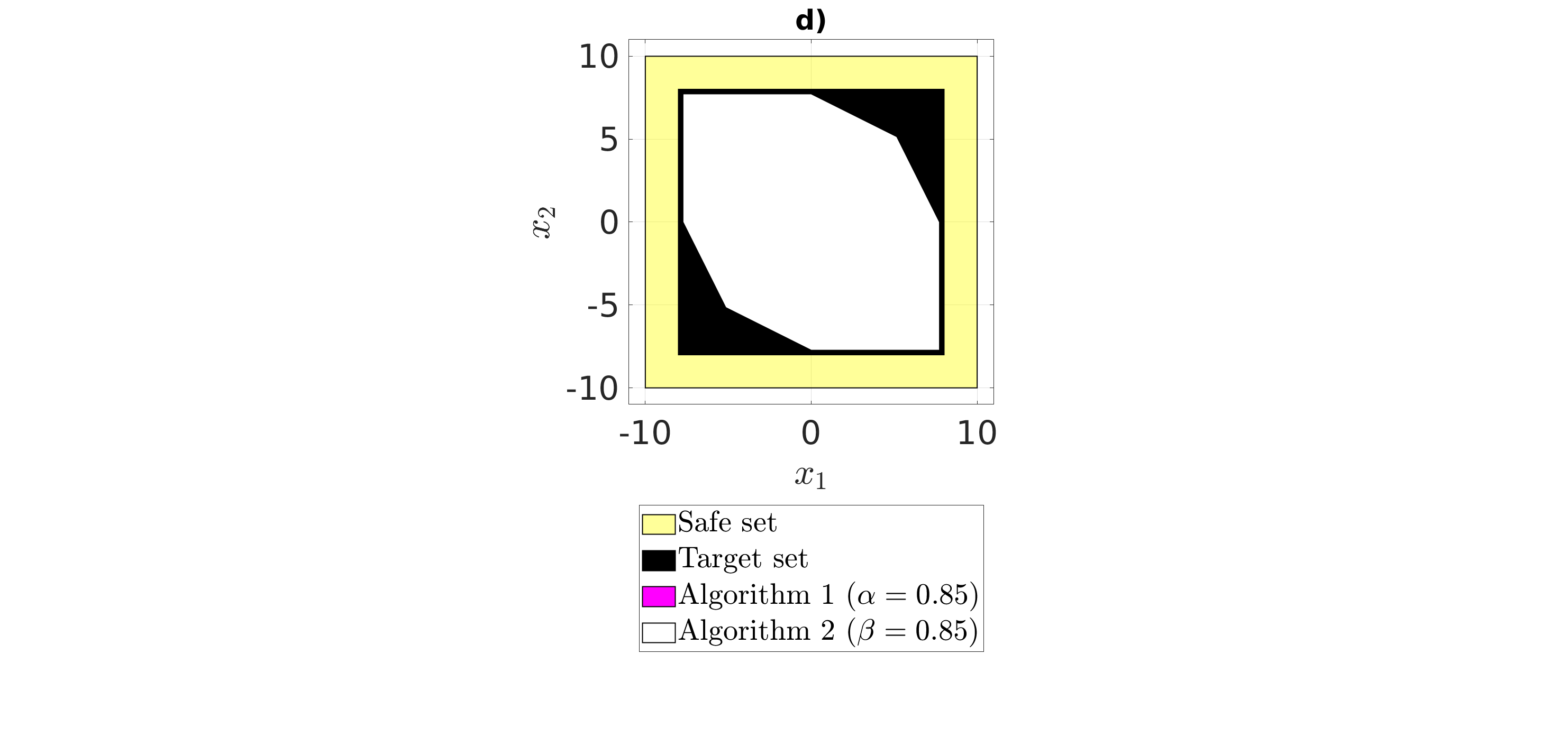
Figure 6: Stochastic reachable sets for a chain of integrators. Figures a) and c) show the stochastic reach sets and their underapproximations for $\alpha\in\{0.6,0.9\}$ for $n=2$ and $n=40$, respectively. Figures b) and d) show the underapproximative interpolations for $n=2$ and $n=40$, respectively. For $n=40$, the plots show the initial state $\overline{x}_{0}=[x_{1}\ x_{2}\ 0\ \cdots\ 0]^{\top}$. We choose $\overline{x}_{c}$ (30) for $\overline{x}_{\mathrm{anchor}}$.

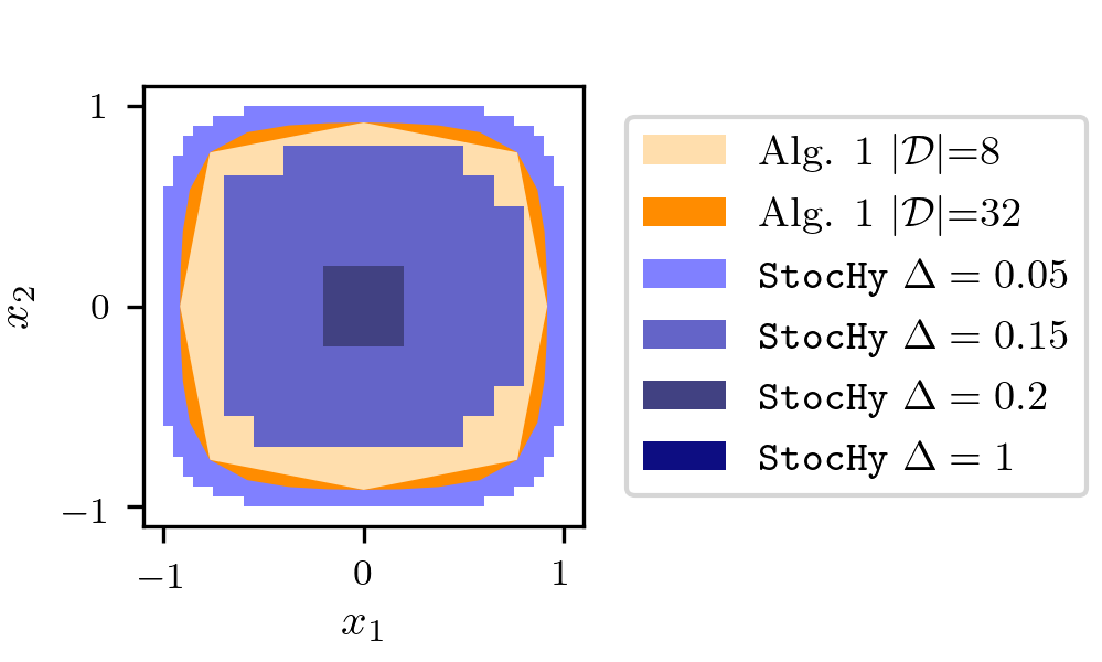
Figure 7: Stochastic reach sets for $\alpha=0.6$ and $n=2$. (Top) Algorithm 1 produced a larger underapproximation than StocHy for $\Delta\in\{1,0.2,0.15\}$, but a smaller underapproximation for $\Delta=0.05$. StocHy returned an empty set for $\Delta=1$. (Bottom) As expected, computational effort of Algorithm 1 and StocHy increases with higher fidelity.

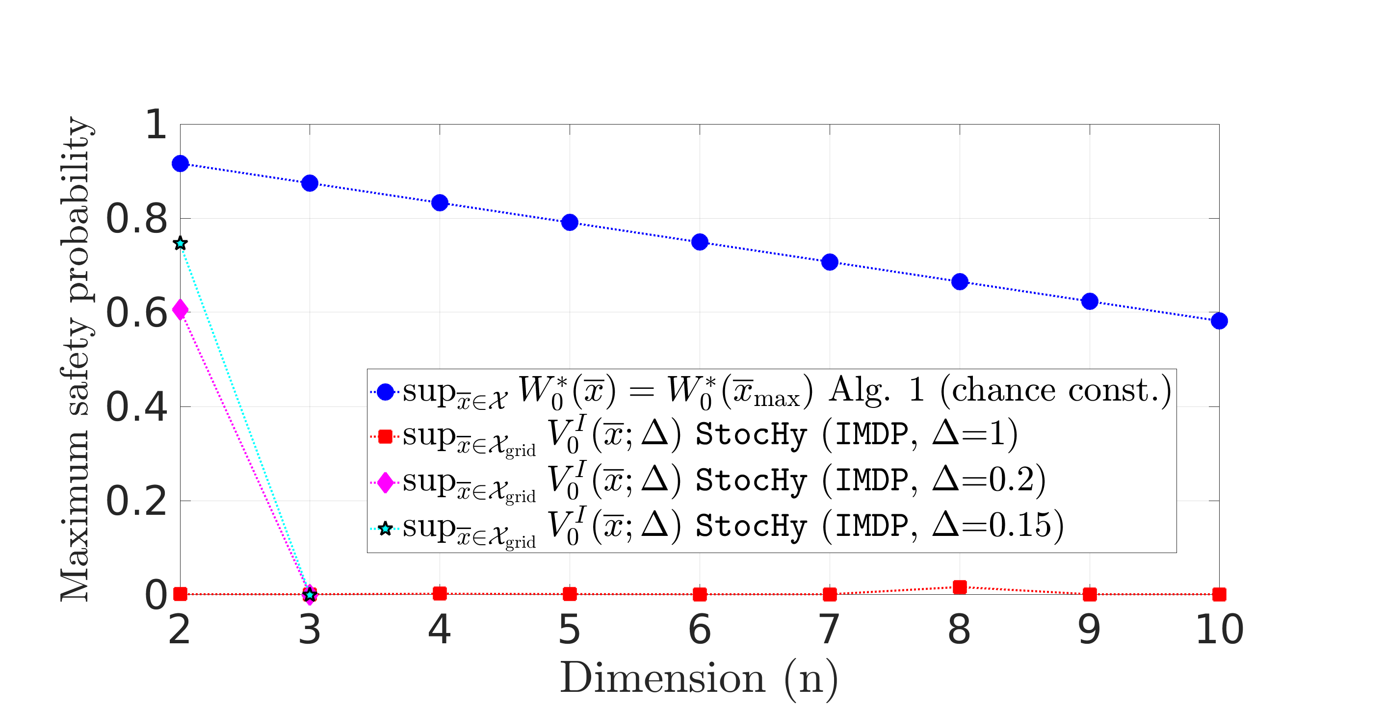
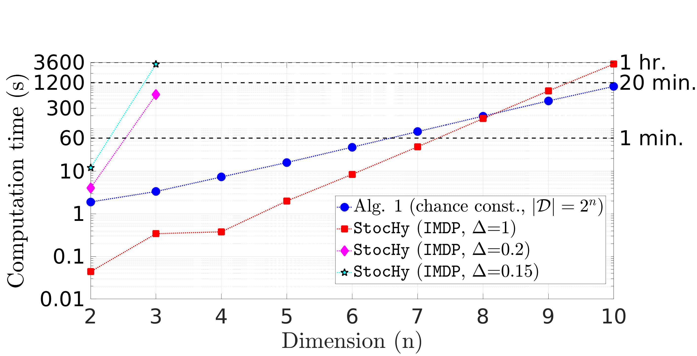
Figure 8: Comparison of Algorithm 1 with StocHy for various $n$. (Left) Algorithm 1 generates higher maximal safety probabilities than StocHy; for $n\geq 3$, StocHy returns trivial underapproximations, despite reductions in grid step size. (Right) Computation of Algorithm 1 with $|\mathcal{D}|=2^{n}$ scales significantly better than StocHy for fine grids, and comparably for coarse grids.

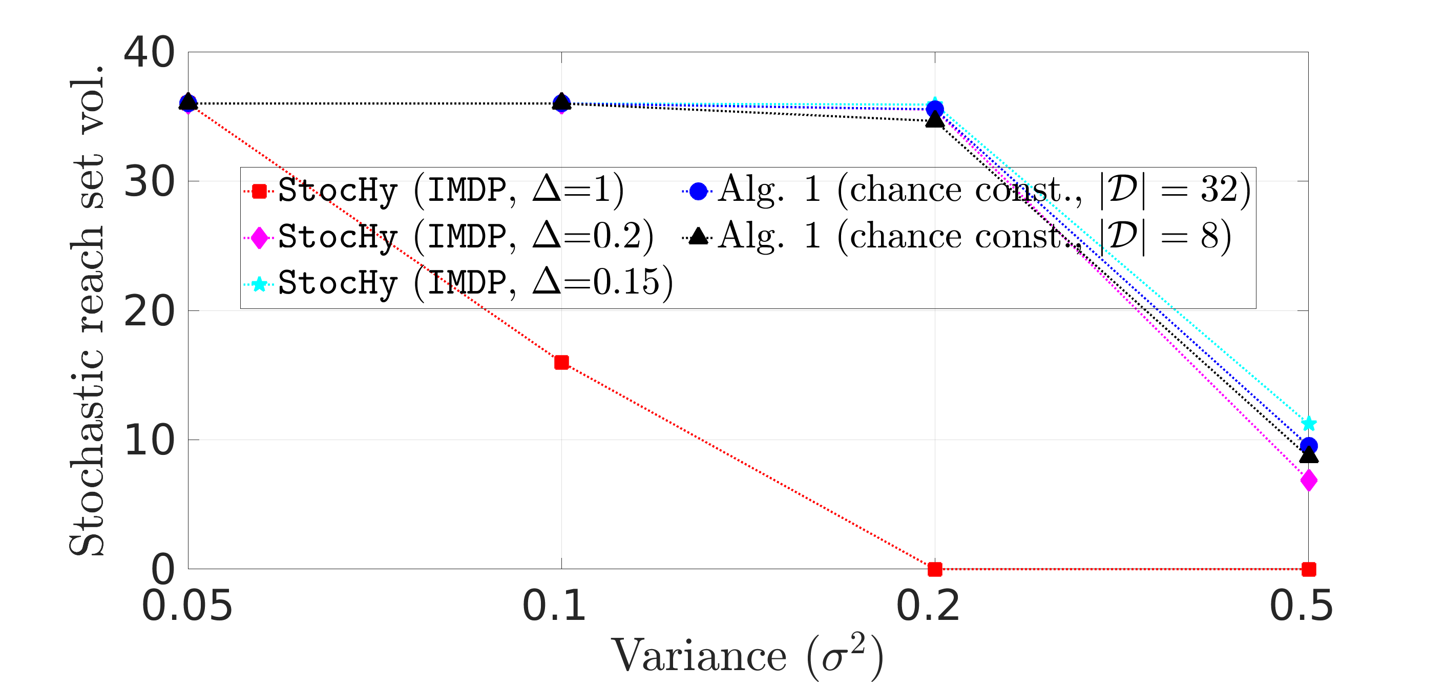
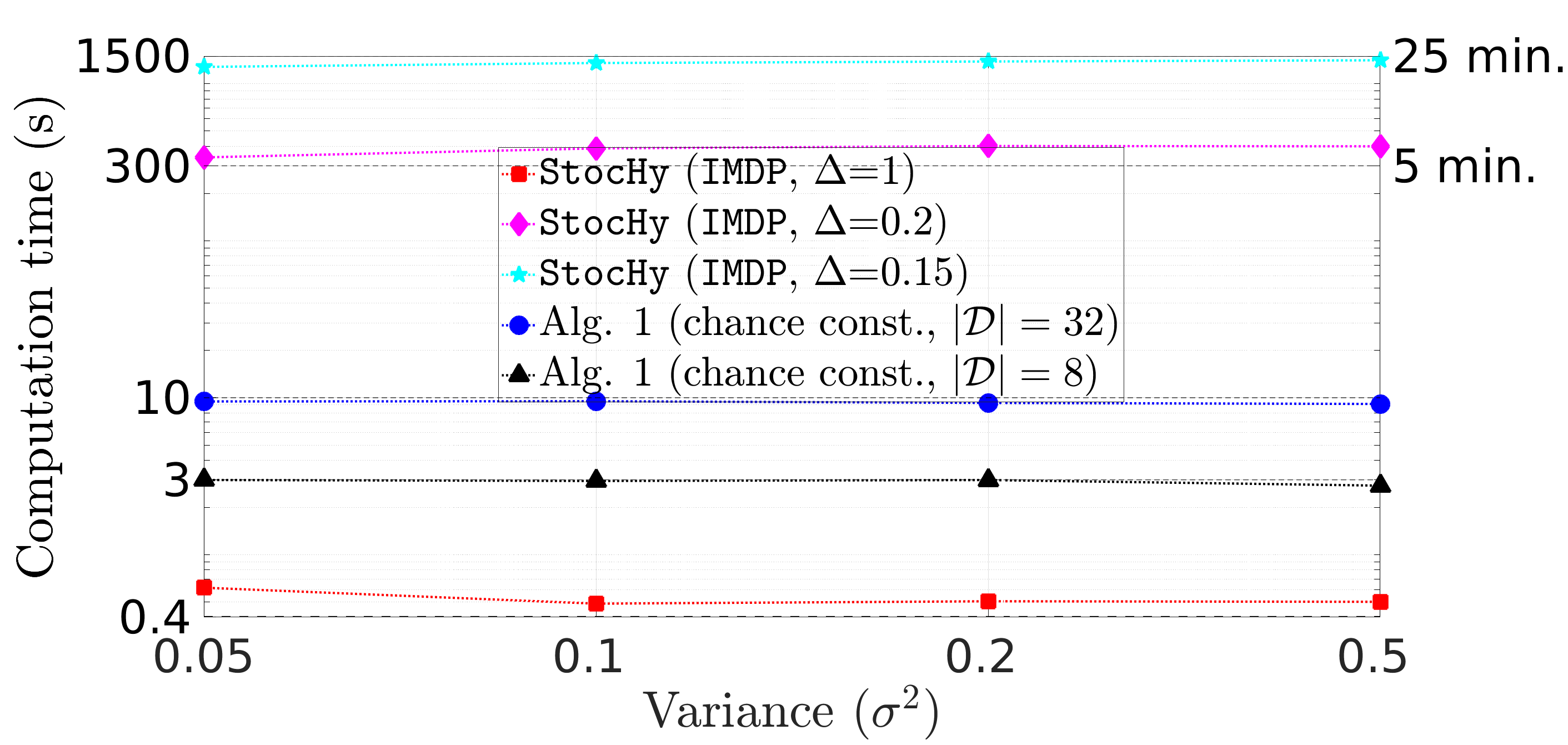
Figure 9: Comparison of Algorithm 1 with StocHy for various $\sigma^{2}$ and $n=2$. (Left) Algorithm 1 exhibits a lower degree of conservativeness (larger volume) than StocHy, except for a fine grid $\Delta=0.15$. (Right) The computational effort required by Algorithm 1 is two orders of magnitude ($3-10$ seconds as compared to $300-1500$ seconds) lower than StocHy for $\Delta\in\{0.15,0.2\}$.

5.2 Comparison of Algorithm 1 and StocHy

StocHy solves stochastic viability or reach-avoid problems for stochastic hybrid systems [9, 10] via abstraction and dynamic programming. StocHy computes look-up tables $V^{I}_{0}(x;\Delta):\mathcal{X}_{\mathrm{grid}}\to[0,1]$ defined over a grid $\mathcal{X}_{\mathrm{grid}}\subset\mathcal{X}$ with step size $\Delta>0$. We focus on the IMDP implementation of StocHy, since its solution $V^{I}_{0}(x;\Delta)$ lower bounds the true safety probability (5). The alternative implementation, FAUST² [38] scales more poorly and is slower than IMDP [10]. Table 4 summarizes the differences between SReachTools (which implements Algorithm 1) and StocHy. Because IMDP cannot accommodate continuous control input and time-varying target sets, we consider the uncontrolled system

$$\boldsymbol{x}_{k+1} =0.8\boldsymbol{x}_{k}+\boldsymbol{w}_{k}$$ (46)

with state $\boldsymbol{x}_{k}\in\mathbb{R}^{n}$ and disturbance $\boldsymbol{w}_{k}\sim\mathcal{N}(0,\sigma^{2}I_{n})$, and compute the $0.6$-stochastic viability set for $N=10$ and $\mathcal{T}_{k}=\mathcal{S}$.

Table 4: Capabilities of SReachTools and StocHy.

Property	SReachTools	StocHy
System model	Linear time-varying	Hybrid time- invariant
Specification	Reachability of target tube (6)	Viability or reach-avoid
Underapproximative verification	✓	✓
Underapproximative controller synthesis	✓
Controller type	Open-loop or affine feedback	Grid based state feedback

Advantage of grid-free approach: To compare the stochastic reach sets produced by Algorithm 1 (grid-free) to the sets produced by StocHy (grid-based), we chose $\sigma^{2}=0.05$, $n=2$, $\mathcal{S}=[-1,1]^{2}$, and varied the grid step size $\Delta\in\{0.05,0.15,0.2,1\}$. Figure 7 shows that the sets generated by Algorithm 1 are less conservative (larger volume) than StocHy, except when a very fine grid ($\Delta=0.05$) is used. However, StocHy was two orders of magnitude slower than Algorithm 1 for $\Delta=0.05$.

Scalability evaluation: We compared the maximal safety probabilities, $\sup_{\overline{x}\in\mathcal{X}}W_{0}^{\ast}(\overline{x})$ via Algorithm 1, and $\sup_{\overline{x}\in\mathcal{X}_{\mathrm{grid}}}V_{0}^{I}(\overline{x};\Delta)$ via StocHy, with $\sigma^{2}=0.05$ and $\mathcal{S}=[-1,1]^{n}$. Figure 8 (left) shows that StocHy is more conservative, as it consistently computes a lower maximal safety probability than Algorithm 1, despite reductions in grid size ($\Delta\in\{0.15,0.2\}$). Indeed, StocHy generated trivial underapproximations for $n\geq 3$, and for $n\geq 4$, the computational cost for $\Delta\in\{0.15,0.2\}$ was prohibitive (Figure 8 (right)). Computationally, Algorithm 1 scales comparably to StocHy for a coarse grid ($\Delta=1$), and significantly better than StocHy for finer grids ($\Delta\in\{0.15,0.2\}$). We used chance constraint approach with $|\mathcal{D}|=2^{n}$ and $\overline{x}_{\mathrm{max}}$ as $\overline{x}_{c}$ in Algorithm 1.

Effect of disturbance variance: We evaluate the volume of the stochastic reach set for $\sigma^{2}\in\{0.05,0.1,0.2,0.5\}$ for $n=2$ and $\mathcal{S}=[-3,3]^{2}$, via Algorithm 1 and StocHy, in Figure 9. As expected, the reach set volume decreases as the disturbance variance increases. Algorithm 1 produces stochastic reach sets of similar volume as that of StocHy at finer grids $\Delta\in\{0.15,0.2\}$, in significantly lower computation time. StocHy is faster than Algorithm 1 for $\Delta=1$, but is significantly more conservative.

In summary, we observe empirically that Algorithm 1 tends to be less conservative and computationally faster than StocHy.

5.3 Spacecraft rendezvous

We consider two spacecraft in the same elliptical orbit. One spacecraft, referred to as the deputy, must approach and dock with another spacecraft, referred to as the chief, while remaining in a line-of-sight cone, in which accurate sensing of the other vehicle is possible. The relative dynamics are described by the Clohessy-Wiltshire-Hill (CWH) equations [46] with an additive stochastic noise to account for model uncertainties,

$$\ddot{x}-3\omega x-2\omega\dot{y}=m_{d}^{-1}F_{x},\quad\ddot{y}+2\omega\dot{x}=m_{d}^{-1}F_{y}.$$ (47)

The chief is located at the origin, the position of the deputy is $x,y\in\mathbb{R}$, $\omega=\sqrt{\Gamma/R_{0}^{3}}$ is the orbital frequency, $\Gamma$ is the standard gravitational parameter, and $R_{0}$ is the orbital radius of the spacecraft. See [27, 19] for further details.

We define the state as $z=[x,y,\dot{x},\dot{y}]\in\mathbb{R}^{4}$ and input as $u=[F_{x},F_{y}]\in\mathcal{U}=[-u_{M},u_{M}]^{2}\subseteq\mathbb{R}^{2}$ for some $u_{M}>0$. We discretize the dynamics (47) in time to obtain

$$\overline{z}_{k+1}=A\overline{z}_{k}+B\overline{u}_{k}+\boldsymbol{w}_{k},$$

with a Gaussian disturbance $w_{k}\in\mathbb{R}^{4}$ with zero mean, and covariance $10^{-4}\times\mbox{diag}(1,1,5\times 10^{-4},5\times 10^{-4})$. For a time horizon of $N=5$, we define the target tube

$$\mathcal{T}_{5} =\left\{\overline{z}\in\mathbb{R}^{4}:|z_{1}|\leq 0.1,-0.1\leq z_{2}\leq 0,|z_{3}|\leq 0.01,|z_{4}|\leq 0.01\right\},\mbox{ and }$$

$$\mathcal{T}_{k} =\left\{\overline{z}\in\mathbb{R}^{4}:2\leq|z_{1}|\leq-z_{2},|z_{3}|\leq 0.5,|z_{4}|\leq 0.5\right\}$$

for $k\in\mathbb{N}_{[0,4]}$. We want to solve the stochastic reach-avoid problem for $\alpha=0.8$ with initial velocity $\dot{x}=\dot{y}=v_{\mathrm{const}}$ km/s for two scenarios: P1) $v_{\mathrm{const}}=0$ and $u_{M}=0.1$, and P2) $v_{\mathrm{const}}=0.01$ and $u_{M}=0.01$.

We construct underapproximative stochastic reach sets using Algorithm 1 with convex chance constraint and Fourier transform approaches. We compare these results with the grid-based approach proposed in [27]. In [27], the problem $\sup_{\overline{U}\in\mathcal{U}^{N}}W_{0}(\overline{x},\overline{U})$ is solved in a chance-constrained formulation using MATLAB’s fmincon for $\overline{x}\in\mathcal{X}_{\mathrm{grid}}$ (over the visible area) with grid step-size $\Delta=0.01$. Figure 10 shows the sets, and Table 5 shows the computation time, and the statistics of the approximation error of the open-loop maximal reach probability using Monte Carlo simulations with $10^{5}$ scenarios at the vertices of $\underline{\mathcal{K}^{\rho^{\ast}}_{0}}(\alpha,\mathscr{T},\mathcal{D})$. Due to the dimensionality, this problem is intractable via dynamic programming. This problem is also hard for abstraction-based techniques like StocHy [9], since $\mathcal{T}_{k}$ are not axis-aligned hypercubes.

Figure 10: Spacecraft rendezvous and docking problem. Comparison of Algorithm 1 using chance constraints and Fourier transform approaches and the grid-based solution [27]. Initial velocity is zero for case P1 (top), and non-zero for case P2 (bottom). We choose $|\mathcal{D}|=32$ and $\overline{x}_{c}$ (30) for $\overline{x}_{\mathrm{anchor}}$.

Table 5: Computation time (seconds) and approximation error in $W_{0}^{\ast}(\overline{x}_{\mathrm{anchor}}+\theta_{i}^{\ast}\overline{d}_{i})$ for each $i\in\mathcal{D}$. The approximation error is the difference of the open-loop reach probability estimated using Monte Carlo simulation ($10^{5}$ particles) and the optimal solution of (35) at each direction vector $\overline{d}_{i}$. Only the visible area in [27] is gridded for P2, to avoid time-out ($<3$ hours).

Fig.	Chance-constraint			Fourier transform			[27]
	Time	Error at vertex		Time	Error at vertex		Time
	(s)	mean	std.	(s)	mean	std.	(s)
10, top	$9.84$	$0.037$	$0.028$	$679.93$	$0.006$	$0.007$	$8369.84$
10, bottom	$10.98$	$0.017$	$0.004$	$842.77$	$0.015$	$0.006$	$764.92$
11	$32.19$	$0.128$	$0.036$

Algorithm 1 implemented using convex chance constraint approach (SReachSetCcO in SReachTools) is significantly faster (two orders of magnitude) than the Fourier transform approach (SReachSetGpO in SReachTools), since it relies on a standard conic solver (like MOSEK [4] or CVX) instead of a gradient-free nonlinear optimization solver (MATLAB’s patternsearch). On the other hand, the Fourier transform approach typically provides a larger underapproximative reach set. This is because it approximates $W_{0}(\cdot)$ directly, instead of relying using Boole’s inequality for an underapproximation, and we initialize MATLAB’s patternsearch with the solution obtained from the convex chance constraint implementation. Algorithm 1 with chance constraints is two to four orders of magnitude faster than [27], since it relies on convex solvers and does not require gridding, and is more computationally robust. We also used Monte-Carlo simulations from each of the vertices of the computed polytopes to validate that the safety prescriptions of Algorithm 1 implemented using convex chance constraints or Fourier transform is underapproximative (approximation error in Table 5 has a positive mean).

5.4 Dubin’s vehicle: Linear time-varying system with time-varying target

We consider the problem of driving a Dubin’s vehicle under a known turning rate sequence while staying within a target tube. When the turning rate sequence and the initial heading are known, the resulting sequence of heading angles can be constructed a priori. The corresponding linear time-varying vehicle dynamics are,

$$\boldsymbol{x}_{k+1} =\boldsymbol{x}_{k}+\left[\begin{array}[]{c}T_{s}\cos(\varphi_{0}+T_{s}\sum_{j=0}^{k-1}\omega_{j})\\ T_{s}\sin(\varphi_{0}+T_{s}\sum_{j=0}^{k-1}\omega_{j})\\ \end{array}\right]u_{k}+\boldsymbol{\eta}_{k}$$ (50)

with position $\boldsymbol{x}_{k}\in\mathbb{R}^{2}$, heading velocity $u_{k}\in[0,u_{M}]$, sampling time $T_{s}$, known initial heading $\varphi_{0}$, time horizon $N$, known sequence of turning rates $\{\omega_{k}\}_{k=0}^{N-1}$, and a Gaussian random process $\boldsymbol{\eta}_{k}\sim\mathcal{N}(\overline{\mu}_{\boldsymbol{\eta}},\Sigma_{\boldsymbol{\eta}})$. For some fraction $\delta\in(0,1]$, let ${\{\overline{c}_{k}\}}_{k=0}^{N-1}$ be the resulting nominal trajectory of (50) associated with a fixed heading velocity $u_{k}=u_{M}\delta,\ \forall k\in\mathbb{N}_{[0,N]}$.

We choose the parameters $N=50$, $T_{s}=0.1$, $\omega_{k}=0.2\pi\ \forall k\in\mathbb{N}_{[0,N-1]}$, $\varphi_{0}=0.1\pi$, $u_{M}=10$, $\delta=0.7$, $\overline{\mu}_{\boldsymbol{\eta}}=\overline{0}_{2}$, and $\Sigma_{\boldsymbol{\eta}}=10^{-3}I_{2}$. We wish to compute the $0.8$-level stochastic reach set of the target tube $\mathcal{T}_{k}=\mathrm{Box}\left(\overline{c}_{k},4\exp\left({\frac{-k}{N_{c}}}\right)\right),\ \forall k\in\mathbb{N}_{[0,N]}$ where $N_{c}=100$ is the decay time constant and $\mathrm{Box}(\overline{c}_{k},a)\subset\mathbb{R}^{2}$ is an axis-aligned box centered around $\overline{c}_{k}$ with side $2a,\ a>0$. StocHy [9] does not support time-varying dynamics.

Figure 11 shows the underapproximative open-loop stochastic reach set computed by Algorithm 1 (convex chance constrained approach). The computed open-loop controller contains the spread of the simulated trajectories within the target tube, as shown for one of the vertices of $\underline{\mathcal{K}^{\rho^{\ast}}_{0}}(\alpha,\mathscr{T},\mathcal{D})$. Due to the long time horizon and the large state space, grid-based dynamic programming is infeasible. Table 5 shows that the conservatism (approximation error has a positive and large mean) in the computed lower bounds at the vertices, due to Boole’s inequality.

Figure 11: Stochastic reach set of a Dubin’s vehicle with a target tube. The cyan polytopes show the spread of the trajectories ($10^{5}$ scenarios) in Monte Carlo simulation, under the open-loop controller from Algorithm 1. We choose $|\mathcal{D}|=16$ and $\overline{x}_{c}$ (30) for $\overline{x}_{\mathrm{anchor}}$.

6 Conclusions

In this paper, we have characterized the properties of the stochastic reachability problem of a target tube, that guarantee existence and closed, compact, and convex stochastic reach set. By establishing convexity properties, we constructed an underapproximation of the stochastic reach set via interpolation. Finally, we proposed a scalable, grid-free, and anytime algorithm that provides an open-loop controller-based polytopic underapproximation of the stochastic reach set.

Appendix A Proofs for Propositions 4, 6, 7, and 13

A.1 Proof of Proposition 4

For any $k\in\mathbb{N}_{[0,N]}$ and $\overline{x}\in\mathcal{L}^{\pi^{\ast}}_{k}(\alpha,\mathscr{T})$, $V_{k}^{\ast}(\overline{x})\geq\alpha$. By (9), we have $1_{\mathcal{T}_{k}}(\overline{x})\geq V_{k}^{\ast}(\overline{x})\geq\alpha>0\Rightarrow\overline{x}\in\mathcal{T}_{k}$, which implies $\mathcal{L}^{\pi^{\ast}}_{k}(\alpha,\mathscr{T})\subseteq\mathcal{T}_{k}$. The boundedness of $\mathcal{L}^{\pi^{\ast}}_{k}(\alpha,\mathscr{T})$ follows by definition [40, Defn. 12.5.3]. $\blacksquare$

A.2 Proof of Proposition 6

a) (By induction) By definition, the indicator functions $1_{\mathcal{T}_{k}}(\cdot)$ for all $k\in\mathbb{N}_{[0,N]}$ are Borel-measurable since $\mathcal{T}_{k}$ are Borel sets. Consequently, $V_{N}^{\ast}(\cdot)$ is Borel-measurable by (8a).

Consider the base case $k=N-1$. Since $V_{N}^{\ast}(\cdot)$ is Borel-measurable (by above) and bounded (by (9)) and the stochastic kernel is input-continuous, the function $\int_{\mathcal{X}}V_{N}^{\ast}(\overline{y})Q_{N-1}(d\overline{y}|\overline{x},\overline{u})$ is continuous over $\mathcal{U}$ for each $\overline{x}\in\mathcal{X}$ by Definition 5a. Since continuity implies upper semi-continuity [7, Lem. 7.13 (b)] and $\mathcal{U}$ is compact, an optimal Borel-measurable input map $\mu_{N-1}^{\ast}(\cdot)$ exists and $\int_{\mathcal{X}}V_{N}^{\ast}(\overline{y})Q_{N-1}(d\overline{y}|\overline{x},\mu_{N-1}^{\ast}(\overline{x}))$ is Borel-measurable over $\mathcal{X}$ by the measurable selection theorem [23, Thm. 2]. Finally, $V^{\ast}_{N-1}(\cdot)$ is Borel-measurable since the product operator preserves Borel-measurability [40, Cor. 18.5.7].

For the case $k\in\mathbb{N}_{[0,N-2]}$, assume for induction that $V_{k+1}^{\ast}(\cdot)$ is Borel-measurable. By the same arguments as above, a Borel-measurable $\mu_{k}^{\ast}(\cdot)$ exists and $V_{k}^{\ast}(\cdot)$ is Borel-measurable.

For every $k\in\mathbb{N}_{[0,N]}$, the set $\mathcal{L}^{\pi^{\ast}}_{k}(\alpha,\mathscr{T})$ is well-defined for $\alpha\in[0,1]$, since $V_{k}^{\ast}(\cdot)$ is well-defined.

b) Since continuous stochastic kernels are input-continuous, the results of Proposition 6a hold. We know that $V_{k}^{\ast}(\cdot)$ is zero (and thereby, continuous) in the complement of $\mathcal{T}_{k}$ from (8a) and (8b). Also, (8a) shows that $V_{N}(\cdot)$ is one (and thereby, continuous) in the relative interior of $\mathcal{T}_{N}$. We will show that $\int_{\mathcal{X}}V_{k+1}^{\ast}(\overline{y})Q_{k}(d\overline{y}|\overline{x},\mu_{k}^{\ast}(\overline{x}))$ is continuous over $\mathcal{X}$ for every $k\in\mathbb{N}_{[0,N-1]}$. Consequently, $V_{k}^{\ast}(\overline{x})$ is continuous over the relative interior of $\mathcal{T}_{k}$ for any $k\in\mathbb{N}_{[0,N-1]}$ by (8b), which completes the proof.

The function $\int_{\mathcal{X}}V_{k+1}^{\ast}(\overline{y})Q_{k}(d\overline{y}|\overline{x},\overline{u})$ is continuous over $\mathcal{X}\times\mathcal{U}$ for every $k\in\mathbb{N}_{[0,N-1]}$ by Definition 5b, continuous stochastic kernel $Q_{k}$, and Borel-measurability (Proposition 6a) and boundedness (9) of $V_{k+1}^{\ast}(\cdot)$. Using induction and [7, Prop. 7.32], we conclude the existence of $\mu_{k}^{\ast}(\cdot)$ for each $k\in\mathbb{N}_{[0,N-1]}$, such that $\int_{\mathcal{X}}V_{k+1}^{\ast}(\overline{y})Q_{k}(d\overline{y}|\overline{x},\mu_{k}^{\ast}(\overline{x}))$ is lower and upper semi-continuous (thereby, continuous) over $\mathcal{X}$.$\blacksquare$

A.3 A lemma used in the proof of Proposition 7

Lemma 16.

Let the system dynamics $f_{k}(\cdot),\ \forall k\in\mathbb{N}_{[0,N-1]}$ be continuous over $\mathcal{X}\times\mathcal{U}\times\mathcal{W}$, sets $\mathcal{X}$ and $\mathcal{U}$ be closed. For every bounded, non-negative, and u.s.c. function $h:\mathcal{X}\rightarrow\mathbb{R}$ and $k\in\mathbb{N}_{[0,N-1]}$, $\int_{\mathcal{X}}h(\overline{y})Q_{k}(d\overline{y}|\overline{x},\overline{u})$ is u.s.c. over $\mathcal{X}\times\mathcal{U}$.

Proof: By (4), we write $\int_{\mathcal{X}}h(\overline{y})Q_{k}(d\overline{y}|\overline{x},\overline{u})$ as the Lebesgue integral of $h(f_{k}(\overline{x},\overline{u},\overline{w}))$ over $\mathcal{W}$, with respect to the probability measure $\mathbb{P}_{\boldsymbol{w},k}$ [34, Sec. 1.23],

$$\int_{\mathcal{X}}h(\overline{y})Q_{k}(d\overline{y}|\overline{x},\overline{u})=\int_{\mathcal{W}}h(f_{k}(\overline{x},\overline{u},\overline{w}))d\mathbb{P}_{\boldsymbol{w},k}.$$ (51)

Note that $h(f_{k}(\overline{x},\overline{u},\overline{w}))$ is u.s.c. over $\mathcal{X}\times\mathcal{U}\times\mathcal{W}$, since the composition of a u.s.c. function with a continuous function is u.s.c.  [33, Ex. 1.4]. Additionally, $h(f_{k}(\overline{x},\overline{u},\overline{w}))$ is bounded and non-negative, since $h(\cdot)$ is bounded and non-negative. If $L\in\mathbb{R}$ is an upper bound of $h(\cdot)$, then $L-h(f_{k}(\overline{x},\overline{u},\overline{w}))$ is non-negative and lower semi-continuous over $\mathcal{X}\times\mathcal{U}$ for every $\overline{w}\in\mathcal{W}$. By Borel-measurability of $h$, $h(f_{k}(\overline{x},\overline{u},\boldsymbol{w}))$ is Borel-measurable with respect to $(\mathcal{X}\times\mathcal{U}\times\mathcal{W})$. From Fatou’s lemma [13, Sec. 6.2, Thm. 2.1] and the fact that $L-h(f_{k}(\overline{x},\overline{u},\overline{w}))$ is lower semi-continuous, Borel-measurable, and non-negative, we have

$$\liminf_{i}\int_{\mathcal{X}}(L-h(f_{k}(\overline{x}_{i},\overline{u}_{i},\overline{w})))d\mathbb{P}_{\boldsymbol{w},k} \geq\int_{\mathcal{X}}\liminf_{i}(L-h(f_{k}(\overline{x}_{i},\overline{u}_{i},\overline{w})))d\mathbb{P}_{\boldsymbol{w},k}$$

$$\geq\int_{\mathcal{X}}(L-h(f_{k}(\overline{x},\overline{u},\overline{w})))d\mathbb{P}_{\boldsymbol{w},k}$$ (52)

By linearity properties of the Lebesgue integral on (52) [40, Prop. 19.2.6c], $\limsup_{i}\int_{\mathcal{X}}h(f_{k}(\overline{x}_{i},\overline{u}_{i},\overline{w}))d\mathbb{P}_{\boldsymbol{w},k}$ is bounded from above by $\int_{\mathcal{X}}h(f_{k}(\overline{x},\overline{u},\overline{w}))d\mathbb{P}_{\boldsymbol{w},k}$, proving that $\int_{\mathcal{X}}h(\overline{y})Q_{k}(d\overline{y}|\overline{x},\overline{u})$ is u.s.c., as desired.   

A.4 Proof of Proposition 7

a) Since $\mathcal{T}_{k}$ and $\mathcal{X}$ are closed, $1_{\mathcal{T}_{k}}(\cdot),\ \forall k\in\mathbb{N}_{[0,N]}$ is u.s.c. over $\mathcal{X}$. Hence, $V_{N}^{\ast}(\cdot)$ is u.s.c. over $\mathcal{X}$.

Consider the base case $k=N-1$. Since $\mathcal{T}_{N}$ is closed, $V_{N}^{\ast}(\cdot)$ is u.s.c., and $V_{N}^{\ast}(\cdot)$ is bounded and non-negative by (9). Hence, $\int_{\mathcal{X}}V_{N}^{\ast}(\overline{y})Q_{N-1}(d\overline{y}|\overline{x},\overline{u})$ is u.s.c. over $\mathcal{X}\times\mathcal{U}$ by Lemma 16. By a selection result for semicontinuous cost functions [7, Prop. 7.33] and compactness of $\mathcal{U}$, an optimal Borel-measurable input map $\mu_{N-1}^{\ast}(\cdot)$ exists and $\int_{\mathcal{X}}V_{N}^{\ast}(\overline{y})Q_{N-1}(d\overline{y}|\overline{x},\mu_{N-1}^{\ast}(\overline{x}))$ is u.s.c. over $\mathcal{X}$. Since upper semicontinuity is preserved under multiplication [32, Props. B.1], $V_{N-1}^{\ast}(\cdot)$ is u.s.c. over $\mathcal{X}$ by (8b).

For the case $k\in\mathbb{N}_{[0,N-2]}$, assume for induction that $V_{k+1}^{\ast}(\cdot)$ is u.s.c.. By the same arguments as above, a Borel-measurable $\mu_{k}^{\ast}(\cdot)$ exists and $V_{k}^{\ast}(\cdot)$ is u.s.c..

For every $k\in\mathbb{N}_{[0,N]}$, the upper semi-continuity of $V_{k}^{\ast}(\cdot)$ implies that the set $\mathcal{L}^{\pi^{\ast}}_{k}(\alpha,\mathscr{T})$ is closed for $\alpha\in[0,1]$.

b) By Propositions 4 and 7a and Heine-Borel theorem. $\blacksquare$

A.5 Proof of Proposition 13

a) Similarly to the proof of Proposition 7 (Appendix A.4).

b) By induction, we have $W_{0}(\overline{x},\overline{U})\leq V_{0}^{\ast}(\overline{x})$ for every $\overline{x}\in\mathcal{X}$ and $\overline{U}\in\mathcal{U}^{N}$. Consequently, $W_{0}^{\ast}(\overline{x})=\sup_{\overline{U}\in\mathcal{U}^{N}}W_{0}(\overline{x},\overline{U})\leq V_{0}^{\ast}(\overline{x})$ by (18b) and the definition of the supremum. Consequently, $\mathcal{K}^{\rho^{\ast}}_{0}(\alpha,\mathscr{T})\subseteq\mathcal{L}^{\pi^{\ast}}_{0}(\alpha,\mathscr{T})$ for every $\alpha\in[0,1]$ by definition.

c) Similarly to the proof of Theorem 8, we can show by induction that $W_{0}(\overline{x}_{0},\overline{U})$ is log-concave in $\mathcal{X}\times\mathcal{U}^{N}$ when $\mathcal{T}_{k}$ is convex and $\psi_{\boldsymbol{w},k}$ is log-concave. Additionally, $\mathcal{U}^{N}$ is convex since $\mathcal{U}$ is convex [8, Sec. 2.3.2]. Hence, (18b) (and thereby (17)) is a log-concave optimization. Since partial supremum over convex sets preserves log-concavity [8, Sec. 3.2, 3.5], $W_{0}^{\ast}(\cdot)$ is log-concave over $\mathcal{X}$.

d) By Proposition 13a and 13c, $\mathcal{K}^{\rho^{\ast}}_{0}(\alpha,\mathscr{T})$ for every $\alpha\in(0,1]$ is convex and closed by (19). By Proposition 10, $\mathcal{L}^{\pi^{\ast}}_{0}(\alpha,\mathscr{T})$ for every $\alpha\in(0,1]$ is convex and compact. The proof follows from the fact that closed subsets of compact sets are compact [40, Cor. 12.5.6]. $\blacksquare$

References

- [1] A. Abate, S. Amin, M. Prandini, J. Lygeros, and S. Sastry. Computational approaches to reachability analysis of stochastic hybrid systems. In Proc. Hybrid Syst.: Comput. & Ctrl., pages 4–17, 2007.
- [2] A. Abate et al. ARCH-COMP20 category report: Stochastic modelling. In Proc. Int’l W. on App. Verification Cont. & Hybrid Syst., pages 76–106, 2020.
- [3] A. Abate, M. Prandini, J. Lygeros, and S. Sastry. Probabilistic reachability and safety for controlled discrete time stochastic hybrid systems. Automatica, 44(11):2724–2734, 2008.
- [4] MOSEK ApS. MOSEK optimization toolbox (9.1.9), 2020.
- [5] D. Bertsekas. Infinite time reachability of state-space regions by using feedback control. IEEE Trans. Autom. Ctrl., 17(5):604–613, 1972.
- [6] D. Bertsekas and I. Rhodes. On the minimax reachability of target sets and target tubes. Automatica, 7(2):233–247, 1971.
- [7] D. Bertsekas and S. Shreve. Stochastic optimal control: The discrete time case. Academic Press, 1978.
- [8] S. Boyd and L. Vandenberghe. Convex optimization. Cambridge Univ. Press, 2004.
- [9] N. Cauchi and A. Abate. StocHy: Automated verification and synthesis of stochastic processes. In Proc. Int’l Conf. Tools & Alg. Constr. & Analysis of Syst., pages 247–264, 2019. https://github.com/natchi92/stochy.
- [10] N. Cauchi, L. Laurenti, M. Lahijanian, A. Abate, M. Kwiatkowska, and L. Cardelli. Efficiency through uncertainty: Scalable formal synthesis for stochastic hybrid systems. In Proc. Hybrid Syst.: Comput. & Ctrl., pages 240–251, 2019.
- [11] D. Chatterjee, E. Cinquemani, and J. Lygeros. Maximizing the probability of attaining a target prior to extinction. Nonlinear Analysis: Hybrid Syst., 5(2):367–381, 2011.
- [12] D. Chatterjee, P. Hokayem, and J. Lygeros. Stochastic receding horizon control with bounded control inputs: A vector space approach. IEEE Trans. Autom. Ctrl., 56(11):2704–2710, 2011.
- [13] Y.S. Chow and H. Teicher. Probability Theory: Independence, Interchangeability, Martingales. Springer New York, 1997.
- [14] S. Dharmadhikari and K. Joag-Dev. Unimodality, convexity, and applications. Elsevier, 1988.
- [15] J. Ding, M. Kamgarpour, S. Summers, A. Abate, J. Lygeros, and C. Tomlin. A stochastic games framework for verification and control of discrete time stochastic hybrid systems. Automatica, 49(9):2665–2674, 2013.
- [16] D. Drzajic, N. Kariotoglou, M. Kamgarpour, and J. Lygeros. A semidefinite programming approach to control synthesis for stochastic reach-avoid problems. In Proc. Int’l W. on App. Verification Cont. & Hybrid Syst., pages 134–143, 2016.
- [17] M. Farina, L. Giulioni, and R. Scattolini. Stochastic linear model predictive control with chance constraints–a review. J. Process Ctrl., 44:53–67, 2016.
- [18] A. Genz. Numerical computation of multivariate normal probabilities. J. Comp. & Graph. Stat., 1(2):141–149, 1992.
- [19] J. Gleason, A. Vinod, and M. Oishi. Underapproximation of reach-avoid sets for discrete-time stochastic systems via Lagrangian methods. In Proc. IEEE Conf. Dec. & Ctrl., pages 4283–4290, 2017.
- [20] M. Grant and S. Boyd. CVX: MATLAB software for disciplined convex programming. http://cvxr.com/cvx.
- [21] J. Gubner. Probability and random processes for electrical and computer engineers. Cambridge Univ. Press, 2006.
- [22] M. Herceg, M. Kvasnica, C.N. Jones, and M. Morari. Multi-Parametric Toolbox 3.0. In Proc. Euro. Ctrl. Conf., pages 502–510, 2013. https://www.mpt3.org/.
- [23] C. Himmelberg, T. Parthasarathy, and F. VanVleck. Optimal plans for dynamic programming problems. Mathematics of Operations Research, 1(4):390–394, 1976.
- [24] N. Kariotoglou, M. Kamgarpour, T. Summers, and J. Lygeros. The linear programming approach to reach-avoid problems for markov decision processes. J. Artificial Intelligence Research, 60:263–285, 2017.
- [25] N. Kariotoglou, K. Margellos, and J. Lygeros. On the computational complexity and generalization properties of multi-stage and stage-wise coupled scenario programs. Syst. & Ctrl. Lett., 94:63–69, 2016.
- [26] T. Kolda, R. Lewis, and V. Torczon. Optimization by direct search: New perspectives on some classical and modern methods. SIAM review, 45(3):385–482, 2003.
- [27] K. Lesser, M. Oishi, and R. Erwin. Stochastic reachability for control of spacecraft relative motion. In Proc. IEEE Conf. Dec. & Ctrl., pages 4705–4712, 2013.
- [28] N. Malone, K. Lesser, M. Oishi, and L. Tapia. Stochastic reachability based motion planning for multiple moving obstacle avoidance. In Proc. Hybrid Syst.: Comput. & Ctrl., pages 51–60, 2014.
- [29] G. Manganini, M. Pirotta, M. Restelli, L. Piroddi, and M. Prandini. Policy search for the optimal control of Markov Decision Processes: A novel particle-based iterative scheme. IEEE Trans. Cybern., 46(11):2643 – 2655, 2015.
- [30] A. Mesbah. Stochastic model predictive control: An overview and perspectives for future research. IEEE Ctrl. Syst. Mag., 36(6):30–44, 2016.
- [31] M. Ono and B. Williams. Iterative risk allocation: a new approach to robust Model Predictive Control with a joint chance constraint. In Proc. IEEE Conf. Dec. & Ctrl., pages 3427–3432, 2008.
- [32] M. Putterman. Markov Decision Processes: Discrete Stochastic Dynamic Programming. John Wiley & Sons, 2005.
- [33] R. Rockafellar and R. Wets. Variational analysis, volume 317. Springer Science & Business Media, 2009.
- [34] W. Rudin. Real and complex analysis. Tata McGraw-Hill, 1987.
- [35] H. Sartipizadeh, A. Vinod, Behçet Açikmese, and M. Oishi. Voronoi partition-based scenario reduction for fast sampling-based stochastic reachability computation of LTI systems. In Proc. Amer. Ctrl. Conf., pages 37–44, 2019.
- [36] J. Skaf and S. Boyd. Design of affine controllers via convex optimization. IEEE Trans. Autom. Ctrl., 55(11):2476–87, 2010.
- [37] S. Soudjani and A. Abate. Probabilistic reach-avoid computation for partially degenerate stochastic processes. IEEE Trans. Autom. Ctrl., 59(2):528–534, 2014.
- [38] S. Soudjani, C. Gevaerts, and A. Abate. FAUST2: Formal Abstractions of Uncountable-STate STochastic processes. In Proc. Int’l Conf. Tools & Alg. Constr. & Analysis of Syst., pages 272–286, 2015.
- [39] S. Summers and J. Lygeros. Verification of discrete time stochastic hybrid systems: A stochastic reach-avoid decision problem. Automatica, 46(12):1951–1961, 2010.
- [40] T. Tao. Analysis II. Hindustan Book Agency, 2 edition, 2009.
- [41] A. Vinod, J. Gleason, and M. Oishi. SReachTools: A MATLAB Stochastic Reachability Toolbox. In Proc. Hybrid Syst.: Comput. & Ctrl., pages 33 – 38, 2019. https://sreachtools.github.io.
- [42] A. Vinod and M. Oishi. Scalable underapproximation for the stochastic reach-avoid problem for high-dimensional LTI systems using Fourier transforms. IEEE Lett.-Contr. Syst. Soc., 1(2):316–321, 2017.
- [43] A. Vinod and M. Oishi. Scalable underapproximative verification of stochastic LTI systems using convexity and compactness. In Proc. Hybrid Syst.: Comput. & Ctrl., pages 1–10, 2018.
- [44] A. Vinod, V. Sivaramakrishnan, and M. Oishi. Piecewise-affine approximation-based stochastic optimal control with Gaussian joint chance constraints. In Proc. Amer. Ctrl. Conf., pages 2942–2949, 2019.
- [45] R. Webster. Convexity. Oxford University Press, 1994.
- [46] W. Wiesel. Spaceflight Dynamics. McGraw-Hill, NY, 1989.
- [47] I. Yang. A dynamic game approach to distributionally robust safety specifications for stochastic systems. Automatica, 94:94–101, 2018.