Draft ]As accepted by PRL

BICEP2 / Keck Array X: Constraints on Primordial Gravitational Waves using Planck, WMAP, and New BICEP2/Keck Observations through the 2015 Season

Abstract

We present results from an analysis of all data taken by the BICEP2/Keck CMB polarization experiments up to and including the 2015 observing season. This includes the first Keck Array observations at 220 GHz and additional observations at 95 & 150 GHz. The $Q/U$ maps reach depths of 5.2, 2.9 and 26 $\mu{\mathrm{K}}_{\mathrm{\mbox{\tiny\sc cmb}}}$ arcmin at 95, 150 and 220 GHz respectively over an effective area of $\approx 400$ square degrees. The 220 GHz maps achieve a signal-to-noise on polarized dust emission approximately equal to that of Planck at 353 GHz. We take auto- and cross-spectra between these maps and publicly available WMAP and Planck maps at frequencies from 23 to 353 GHz. We evaluate the joint likelihood of the spectra versus a multicomponent model of lensed-$\Lambda$CDM+$r$+dust+synchrotron+noise. The foreground model has seven parameters, and we impose priors on some of these using external information from Planck and WMAP derived from larger regions of sky. The model is shown to be an adequate description of the data at the current noise levels. The likelihood analysis yields the constraint $r_{0.05}<0.07$ at 95% confidence, which tightens to $r_{0.05}<0.06$ in conjunction with Planck temperature measurements and other data. The lensing signal is detected at $8.8\sigma$ significance. Running maximum likelihood search on simulations we obtain unbiased results and find that $\sigma(r)=0.020$. These are the strongest constraints to date on primordial gravitational waves.

xyz

Introduction.—It is remarkable that our standard model of cosmology, known as $\Lambda$CDM, is able to statistically describe the observable universe with only six parameters (tensions between high and low redshift probes notwithstanding Planck Collaboration 2018 VI (2018)). Observations of the cosmic microwave background (CMB) Penzias and Wilson (1965) have played a central role in establishing this model and now constrain these parameters to percent-level precision (see most recently Ref. Planck Collaboration 2015 XIII (2016)).

The success of this model focuses our attention on the deep physical mysteries it exposes. Dark matter and dark energy dominate the present-day universe, but we lack understanding of both their nature and abundance. Perhaps most fundamentally, the standard model offers no explanation for the observed initial conditions of the universe: highly uniform and flat with small, nearly scale-invariant, adiabatic density perturbations. Inflation is an extension to the standard model that addresses initial conditions by postulating that the observable universe arose from a tiny, causally-connected volume in a period of accelerated expansion within the first fraction of a nanosecond, during which quantum fluctuations of the spacetime metric gave rise to both the observed primordial density perturbations and a potentially-observable background of gravitational waves (see Ref. Kamionkowski and Kovetz (2016) for a recent review and citations to the original literature).

Probing for these primordial gravitational waves through the faint $B$-mode polarization patterns that they would imprint on the CMB is recognized as one of the most important goals in cosmology today, with the potential to either confirm inflation, and establish its energy scale, or to powerfully limit the space of allowed inflationary models Abazajian et al. (2016). Multiple groups are making measurements of CMB polarization, some focused on the gravitational wave goal at larger angular scales, and others focused on other science at smaller angular scales—examples include Keisler et al. (2015); Louis et al. (2017); POLARBEAR Collaboration et al. (2017); Kusaka et al. (2018).

In principle $B$-mode polarization patterns offer a unique probe of primordial gravitational waves because they cannot be sourced by primordial density perturbations Seljak (1997); Kamionkowski et al. (1997); Seljak and Zaldarriaga (1997). However, in practice there are two sources of foreground: gravitational deflections of the CMB photons in flight leads to a lensing $B$-mode component Zaldarriaga and Seljak (1998), and polarized emission from our own galaxy can also produce $B$-modes. The latter can be separated out through their differing frequency spectral behavior, so extremely sensitive multi-frequency observations are needed to advance the leading constraints on primordial gravitational waves.

Our BICEP/Keck program first reported detection of an excess over the lensing $B$-mode expectation at 150 GHz in Ref. BICEP2 Collaboration I (2014). In a joint analysis using multi-frequency data from the Planck experiment it was shown that most or all of this is due to polarized emission from dust in our own galaxy (BICEP2/Keck and Planck Collaborations, 2015, hereafter BKP). We first started to diversify our own frequency coverage by adding data taken in 2014 with Keck Array at 95 GHz, yielding the tightest previous constraints on primordial gravitational waves (Keck Array and BICEP2 Collaborations VI, 2016, hereafter BK14).

In this letter [hereafter BK15], we advance these constraints using new data taken by Keck Array in the 2015 season including two 95 GHz receivers, a single 150 GHz receiver, and, for the first time, two 220 GHz receivers. This analysis thus doubles the 95 GHz dataset from two receiver-years to four, while adding a new higher frequency band that significantly improves the constraints on the dust contribution over what is possible using the Planck 353 GHz data alone. The constraint on primordial gravitational waves parametrized by tensor to scalar ratio $r$ is improved to $r_{0.05}<0.062$ (95%), disfavoring the important class of inflationary models represented by a $\phi$ potentialKamionkowski and Kovetz (2016); Abazajian et al. (2016).

Instrument and observations.—Keck Array consists of a set of five microwave receivers similar in design to the precursor BICEP2 instrument BICEP2 Collaboration II (2014); Keck Array and BICEP2 Collaborations V (2015). Each receiver employs a $\approx 0.25$ m aperture all cold refracting telescope focusing microwave radiation onto a focal plane of polarized antenna-coupled bolometric detectors BICEP2/Keck and Spider Collaborations (2015). The receivers are mounted on a movable platform (or mount) which scans their pointing direction across the sky in a controlled manner. The detectors are read out through a time-domain multiplexed SQUID readout system. Orthogonally-polarized detectors are arranged as coincident pairs in the focal plane, and the pair-difference timestream data thus traces out changes in the polarization signal from place to place on the sky. The telescopes are located at the South Pole in Antarctica where the atmosphere is extremely stable and transparent at the relevant frequencies. The data are recorded to disk and transmitted back to the US daily for analysis.

To date we have mapped a single region of sky centered at RA 0h, Dec. $-57.5^{\circ}$. From 2010 to 2013, BICEP2 and Keck Array jointly recorded a total of 13 receiver-years of data in a band centered on 150 GHz. Two of the Keck receivers were switched to 95 GHz before the 2014 season, and two more were switched to 220 GHz before the 2015 season. The BK15 data set thus consists of 4/17/2 receiver-years at 95/150/220 GHz respectively.

Maps and Power Spectra—We make maps and power spectra using the same procedures as used for BK14 and previous analyses BICEP2 Collaboration I (2014). Briefly: the telescope timestream data are filtered and then binned into sky pixels with the multiple detector pairs being co-added together using knowledge of their individual pointing directions as the telescope scans across the sky. Maps of the polarization Stokes parameters $Q$ and $U$ are constructed by also knowing the polarization sensitivity angle of each pair as projected onto the sky.

After apodizing to downweight the noisy regions around the edge of the observed area, the $Q/U$ maps are Fourier transformed and converted to the $E/B$ basis in which the primordial gravitational wave signal is expected to be maximally distinct from the standard $\Lambda$CDM signal.

Two details worth noting are the deprojection of leading order temperature to polarization leakage terms, and the adjustment of the absolute polarization angle to minimize the $EB$ cross spectrum. See Ref. BICEP2 Collaboration I (2014) for more information.

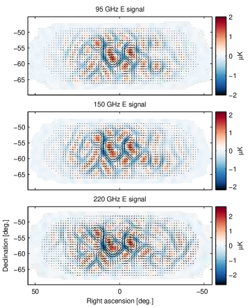
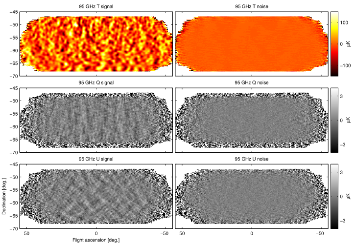
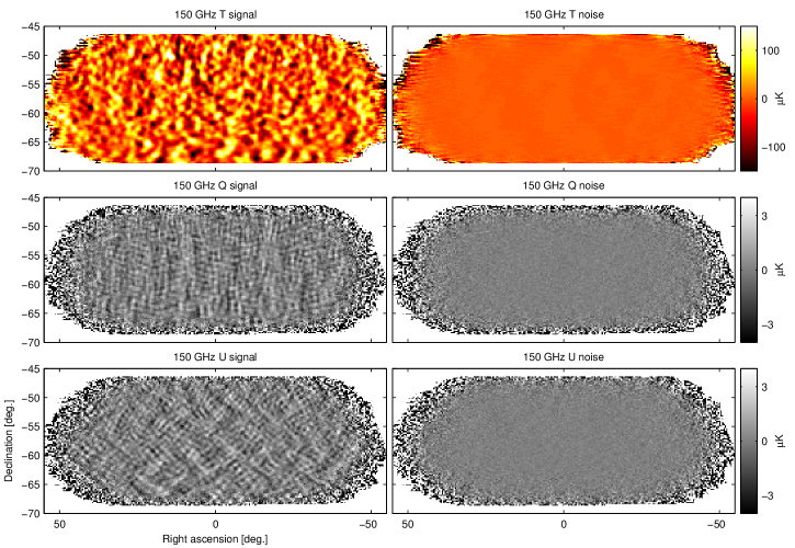
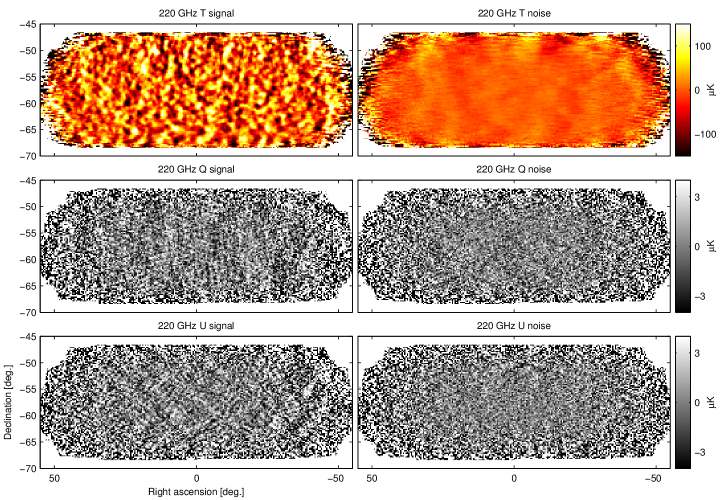
For illustration purposes we can inverse Fourier transform to form $E/B$ maps. Fig. 1 shows $E$-mode maps formed from the 2015 data alone—the data which is being added to the previous data in this analysis. The similarity of the pattern at all three frequencies indicates that $\Lambda$CDM $E$-modes dominate, and that the signal-to-noise is high. The effective area of these maps is $\sim 1$% of the full sky. (See Appendix A for the full set of $T/Q/U$ maps.)

Figure 1: Maps of degree angular scale $E$-modes ($50<\ell<120$) at three frequencies made using Keck Array data from the 2015 season only. The similarity of the pattern indicates that $\Lambda$CDM $E$-modes dominate at all three frequencies (and that the signal-to-noise is high). The color scale is in $\mu{\mathrm{K}}$, and the range is allowed to vary slightly to (partially) compensate for the decrease in beam size with increasing frequency.

To suppress $E$ to $B$ leakage we use the matrix purification technique which we have developed BICEP2 Collaboration I (2014); Keck Array and BICEP2 Collaobrations VII (2016). We then take the variance within annuli of the Fourier plane to estimate the angular power spectra. To test for systematic contamination we carry out our usual “jackknife” internal consistency tests on the new 95 GHz and 220 GHz data as described in Appendices B and C—the distributions of $\chi$ and $\chi^{2}$ PTE values are consistent with uniform showing no evidence for problems.

In this paper we use the three bands of BICEP2/Keck plus the 23 & 33 GHz bands of WMAP (Bennett et al., 2013) and all seven polarized bands of Planck (Planck Collaboration 2015 I, 2016). We take all possible auto- and cross-power spectra between these twelve bands—the full set of spectra are shown in Appendix D.

Fig. 2 shows the $EE$ and $BB$ auto- and cross-spectra for the BICEP2/Keck bands plus the Planck 353 GHz band which is important for constraining the polarized dust contribution. The spectra are compared to the “baseline” lensed-$\Lambda$CDM+dust model from our previous BK14 analysis. Note that the $BB$ spectra involving 220 GHz were not used to derive this model but agree well with it. The $EE$ spectra were also not used to derive the model but agree well with it under the assumption that $EE/BB=2$ for dust, as it is shown to be close to in Planck analysis of larger regions of sky Planck Collaboration Int. XXX (2016); Planck Collaboration 2018 XI (2018). (Note that many of the BICEP/Keck spectra are sample variance dominated.)

Figure 2: $EE$ and $BB$ auto- and cross-spectra calculated using BICEP2/Keck 95, 150 & 220 GHz maps and the Planck 353 GHz map. The BICEP2/Keck maps use all data taken up to and including the 2015 observing season—we refer to these as BK15. The black lines show the model expectation values for lensed-$\Lambda$CDM, while the red lines show the expectation values of the baseline lensed-$\Lambda$CDM+dust model from our previous BK14 analysis ($r=0$, $A_{\mathrm{d,353}}=4.3$ $\mu{\mathrm{K}^{2}}$, $\beta_{\mathrm{d}}=1.6$, $\alpha_{\mathrm{d}}=-0.4$), and the error bars are scaled to that model. Note that the model shown was fit to $BB$ only and did not use the 220 GHz points (which are entirely new). The agreement with the spectra involving 220 GHz and all the $EE$ spectra (under the assumption that $EE/BB=2$ for dust) is therefore a validation of the model. (The dashed red lines show the expectation values of the lensed-$\Lambda$CDM+dust model when adding strong spectral decorrelation of the dust pattern—see Appendix F for further information.)

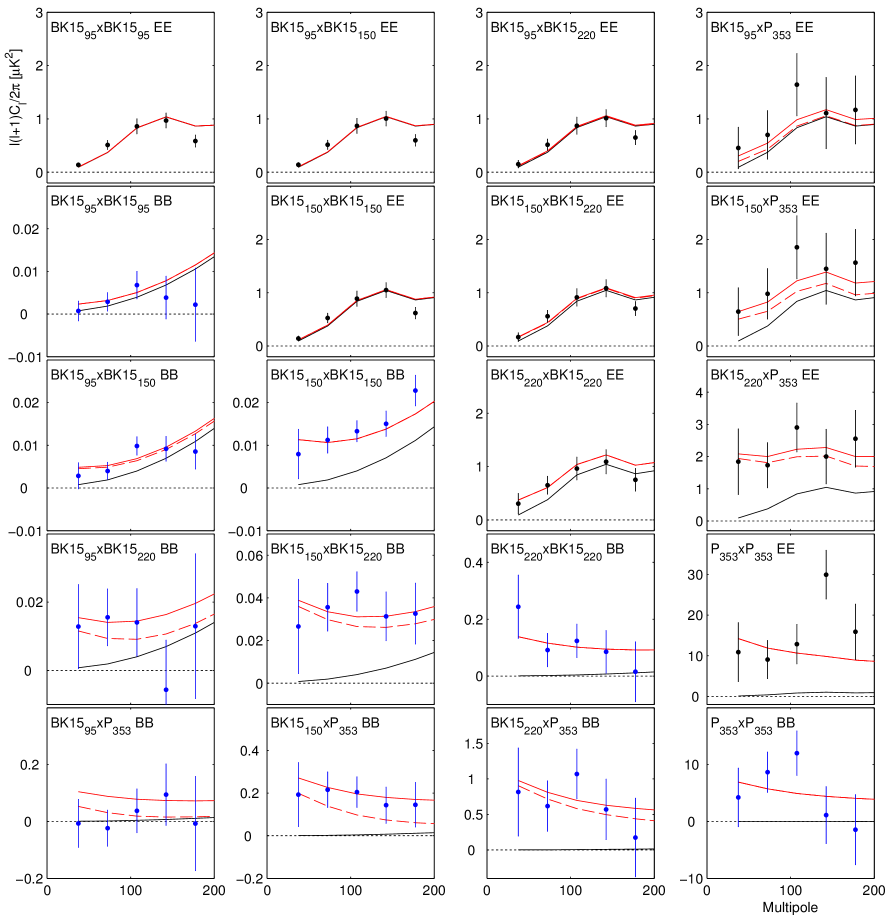
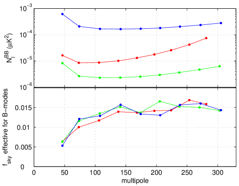
Fig. 3 upper shows the noise spectra (derived using the sign-flip technique BICEP2 Collaboration I (2014); van Engelen et al. (2012)) for the three BK15 bands after correction for the filter and beam suppression. The turn up at low-$\ell$ is partially due to residual atmospheric $1/f$ in the pair-difference data and hence is weakest in the 95 GHz band where water vapor emission is weakest. In an auto-spectrum the quantity which determines the ability to constrain $r$ is the fluctuation of the noise bandpowers rather than their mean. The lower panel therefore shows the effective sky fraction observed as inferred from the fractional noise fluctuation. Together, these panels provide a useful synoptic measure of the loss of information due to noise, filtering, and $EE/BB$ separation in the lowest bandpowers. We suggest that other experiments reproduce this plot for comparison purposes.

Figure 3: Upper: The noise spectra of the BK15 maps for 95 GHz (red), 150 GHz (green) and 220 GHz (blue) after correction for the filtering of signal which occurs due to the beam roll-off and timestream filtering. (Note that no $\ell^{2}$ scaling is applied.) Lower: The effective sky fraction as calculated from the ratio of the mean noise realization bandpowers to their fluctuation $f_{\mathrm{sky}}(\ell)=\frac{1}{2\ell\Delta\ell}\left(\frac{\sqrt{2}\bar{N_{b}}}{\sigma(N_{b})}\right)^{2}$, i.e. the observed number of $B$-mode degrees of freedom divided by the nominal full-sky number. The turn-down at low $\ell$ is due to mode loss to the timestream filtering and matrix purification.

Likelihood Analysis.—We perform likelihood analysis using the methods introduced in BKP and refined in BK14. We use the Hamimeche-Lewis approximation (Hamimeche and Lewis, 2008, hereafter HL) to the joint likelihood of the ensemble of 78 $BB$ auto- and cross-spectra taken between the BICEP2/Keck and WMAP/Planck maps. We compare the observed bandpower values for ${20<\ell<330}$ (9 bandpowers per spectrum) to an eight parameter model of lensed-$\Lambda$CDM+$r$+dust+synchrotron+noise and explore the parameter space using COSMOMC (Lewis and Bridle, 2002) (which implements a Markov chain Monte Carlo). As in our previous analyses the bandpower covariance matrix is derived from 499 simulations of signal and noise, explicitly setting to zero terms such as the covariance of signal-only bandpowers with noise-only bandpowers or covariance of BICEP/Keck noise bandpowers with WMAP/Planck noise bandpowers BICEP2/Keck and Planck Collaborations (2015). The tensor/scalar power ratio $r$ is evaluated at a pivot scale of 0.05 Mpc^-1, and we fix the tensor spectral index $n_{t}=0$. The COSMOMC module containing the data and model is available for download at http://bicepkeck.org. We make only one change to the “baseline” analysis choices of BK14, expanding the prior on the dust/sync correlation parameter. The following paragraphs briefly summarize.

We include dust with amplitude $A_{\mathrm{d,353}}$ evaluated at 353 GHz and ${\ell=80}$. The frequency spectral behavior is taken as a modified black body spectrum with ${T_{\mathrm{d}}=19.6}$ K and ${\beta_{\mathrm{d}}=1.59\pm 0.11}$, using a Gaussian prior with the given $1\sigma$ width, this being an upper limit on the patch-to-patch variation Planck Collaboration Int. XXII (2015); BICEP2/Keck and Planck Collaborations (2015). We note that the latest Planck analysis finds a slightly lower central value of ${\beta_{\mathrm{d}}=1.53}$ Planck Collaboration 2018 XI (2018) (well within our prior range) with no detected trends with galactic latitude, angular scale or $EE$ vs. $BB$. The spatial power spectrum is taken as a power law ${\mathcal{D}_{\ell}\propto\ell^{\alpha_{\mathrm{d}}}}$ marginalizing uniformly over the (generous) range ${-1<\alpha_{\mathrm{d}}<0}$ (where ${\mathcal{D}_{\ell}\equiv\ell\left(\ell+1\right)C_{\ell}/2\pi}$). Planck analysis consistently finds approximate power law behavior of both the $EE$ and $BB$ dust spectra with exponents $\approx-0.4$  Planck Collaboration Int. XXX (2016); Planck Collaboration 2018 XI (2018).

We include synchrotron with amplitude $A_{\mathrm{sync,23}}$ evaluated at 23 GHz (the lowest WMAP band) and $\ell=80$, assuming a simple power law for the frequency spectral behavior ${A_{\mathrm{sync}}\propto\nu^{\beta_{\mathrm{s}}}}$ with a Gaussian prior ${\beta_{\mathrm{s}}=-3.1\pm 0.3}$ (Fuskeland et al., 2014). We note that recent analysis of 2.3 GHz data from S-PASS in conjunction with WMAP and Planck finds $\beta_{\mathrm{s}}=-3.2$ with no detected trends with galactic latitude or angular scale Krachmalnicoff et al. (2018). The spatial power spectrum is taken as a power law ${\mathcal{D}_{\ell}\propto\ell^{\alpha_{\mathrm{s}}}}$ marginalizing over the range ${-1<\alpha_{\mathrm{s}}<0}$ Dunkley et al. (2009). The recent S-PASS analysis finds a value at the bottom end of this range ($\approx-1$) for $BB$ at high galactic latitude.

Finally we include sync/dust correlation parameter $\epsilon$ (called $\rho$ in some other papers Choi and Page (2015); Planck Collaboration 2018 XI (2018); Krachmalnicoff et al. (2018)). In BK14 we marginalized over the range ${0<\epsilon<1}$ but in this paper we extend to the full possible range ${-1<\epsilon<1}$. The latest Planck analysis does not detect sync/dust correlation at high galactic latitude and the $\ell$ range of interest Planck Collaboration 2018 XI (2018).

Results of the baseline analysis are shown in Fig. 4 and yield the following statistics: $r_{0.05}=0.020^{+0.021}_{-0.018}$ ($r_{0.05}<0.072$ at 95% confidence), $A_{\mathrm{d,353}}=4.6^{+1.1}_{-0.9}$ $\mu{\mathrm{K}^{2}}$, and $A_{\mathrm{sync,23}}=1.0^{+1.2}_{-0.8}$ $\mu{\mathrm{K}^{2}}$, ($A_{\mathrm{sync,23}}<3.7$ $\mu{\mathrm{K}^{2}}$at 95% confidence). For $r$, the zero-to-peak likelihood ratio is 0.66. Taking ${\frac{1}{2}\left(1-f\left(-2\log{L_{0}/L_{\rm peak}}\right)\right)}$, where $f$ is the $\chi^{2}$ CDF (for one degree of freedom), we estimate that the probability to get a likelihood ratio smaller than this is 18% if, in fact, $r=0$. As compared to the previous analysis, the likelihood curve for $r$ shifts down slightly and tightens. The $A_{\mathrm{d}}$ curve shifts up very slightly but remains about the same width (presumably saturated at sample variance), and the $A_{\mathrm{sync}}$ curve loses the second bump at zero.

Figure 4: Results of a multicomponent multi-spectral likelihood analysis of BICEP2/Keck+WMAP/Planck data. The red faint curves are the baseline result from the previous BK14 paper (the black curves from Fig. 4 of that paper). The bold black curves are the new baseline BK15 results. Differences between these analyses include adding Keck Array data taken during the 2015 observing season, in particular doubling the 95 GHz sensitivity and adding, for the first time, a 220 GHz channel. (In addition the $\epsilon$ prior is modified.) The upper limit on the tensor-to-scalar ratio tightens to $r_{0.05}<0.072$ at 95% confidence. The parameters $A_{\mathrm{d}}$ and $A_{\mathrm{sync}}$ are the amplitudes of the dust and synchrotron $B$-mode power spectra, where $\beta$ and $\alpha$ are the respective frequency and spatial spectral indices. The correlation coefficient between the dust and synchrotron patterns is $\epsilon$. In the $\beta$, $\alpha$ and $\epsilon$ panels the dashed lines show the priors placed on these parameters (either Gaussian or uniform). Broadening or tightening the uniform prior range on $\alpha_{s}$ and $\alpha_{d}$ results in very small changes, and negligible changes to the $r$ constraint.

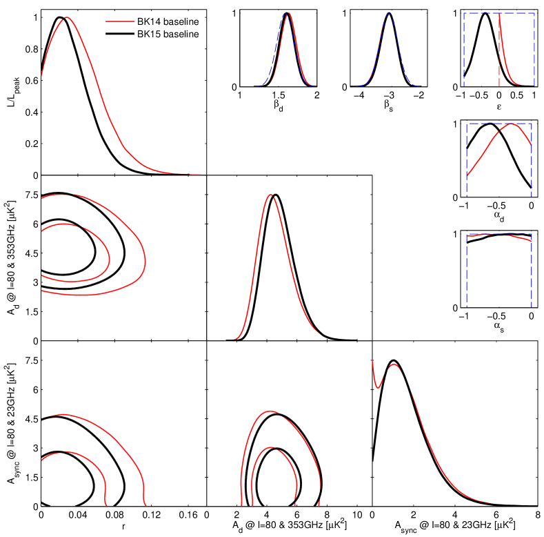
The maximum likelihood model (including priors) has parameters $r_{0.05}=0.020$, $A_{\mathrm{d,353}}=4.7$ $\mu{\mathrm{K}^{2}}$, $A_{\mathrm{sync,23}}=1.5$ $\mu{\mathrm{K}^{2}}$, $\beta_{\mathrm{d}}=1.6$, $\beta_{\mathrm{s}}=-3.0$, $\alpha_{\mathrm{d}}=-0.58$, $\alpha_{\mathrm{s}}=-0.27$, and $\epsilon=-0.38$. This model is an acceptable fit to the data with the probability to exceed (PTE) the observed value of $\chi^{2}$ being 0.19. Thus, while fluctuation about the assumed power law behavior of the dust component is in general expected to be “super-Gaussian” Planck Collaboration 2018 XI (2018), we find no evidence for this at the present noise level—see Appendix D for further details.

We have explored several variations from the baseline analysis choices and data selection and find that these do not significantly alter the results. Removing the prior on $\beta_{\mathrm{d}}$ makes the $r$ constraint curve slightly broader resulting in $r_{0.05}<0.079$ (95%), while using the BICEP/Keck data only shifts the peak position down to zero resulting in $r_{0.05}<0.063$. Concerns have been raised that the known problems with the LFI maps Planck Collaboration 2015 II (2016) might affect the analysis—excluding LFI the $r$ constraint curve peak position shifts down to $r=0.012^{+0.022}_{-0.012}$ ($r_{0.05}<0.065$, with zero-to-peak likelihood ratio of 0.90, and 32% probability to get a smaller value if $r=0$), while the constraint on $A_{\mathrm{sync,23}}$ becomes $2.4^{+1.9}_{-1.4}$ $\mu{\mathrm{K}^{2}}$. The shifts when varying the data set selection (e.g. omitting Planck) are not statistically significant when compared to shifts of lensed-$\Lambda$CDM+dust+noise simulations—see Appendices E.1 and E.2 for further details. Freeing the amplitude of the lensing power we obtain $A_{\rm L}=1.15^{+0.16}_{-0.14}$, and detect lensing at $8.8\sigma$ significance.

The results of likelihood analysis where the parameters are restricted to, and marginalized over, physical values only can potentially be biased. Running the baseline analysis on an ensemble of lensed-$\Lambda$CDM+dust+noise simulations with simple Gaussian dust we do not detect bias. Half of the $r$ constraint curves peak at zero and the CDF of the zero-to-peak likelihood ratios closely follows the idealized analytic expectation. When running maximum likelihood searches on the simulations with the parameters unrestricted we again obtain unbiased results and find that $\sigma(r)=0.020$. See Appendix E.3 for further details.

We extend the maximum likelihood validation study to a suite of third-party foreground models (Thorne et al., 2017; Hensley, 2015; Kritsuk et al., 2017). These models do not necessarily conform to the foreground parameterization which we are using, and when fit to it are in general expected to produce bias on $r$. However, for the models considered we find that such bias is small compared to the instrumental noise—see Appendix E.4.

Spatial variation of the frequency spectral behavior of dust will lead to a decorrelation of the dust patterns as observed in different frequency bands. Since the baseline parametric model assumes a fixed dust pattern as a function of frequency such variation will lead to bias on $r$. Dust decorrelation surely exists at some level—the question is whether it is relevant as compared to the current experimental noise. For the third-party foreground models mentioned above, decorrelation is very small. Since our previous BK14 paper Planck Intermediate Paper L Planck Collaboration Int. L (2017) appeared claiming a detection of relatively strong dust decorrelation between 217 and 353 GHz. This was followed up by Ref. (Sheehy and Slosar, 2018), which analyzed the same data and found no evidence for dust decorrelation, and Planck Intermediate Paper LIV (Planck Collaboration 2018 XI, 2018), which performed a more sophisticated multi-frequency analysis and again found no evidence. In the meantime we added a decorrelation parameter to our analysis framework. Including it only increases $\sigma(r)$ from 0.020 to 0.021, but for the present data set this parameter is partially degenerate with $r$ and including it results in a downward bias on $r$ in simulations—see Appendix F for more details.

By cross correlating against the Planck CO map we find that the contamination of our 220 GHz map by CO is equivalent to $r\sim 10^{-4}$.

Conclusions.—The previous BK14 analysis yielded the constraint $r_{0.05}<0.090$ (95%). Adding the Keck Array data taken during 2015 we obtain the BK15 result $r_{0.05}<0.072$. The distributions of maximum likelihood $r$ values in simulations where the true value of $r$ is zero give $\sigma(r_{0.05})=0.024$ and $\sigma(r_{0.05})=0.020$ for BK14 and BK15 respectively. The BK15 simulations have a median 95% upper limit of $r_{0.05}<0.046$.

Fig. 5 shows the constraints in the $r$ vs. $n_{s}$ plane for Planck 2015 plus additional data ($r_{0.05}<0.12$) and when adding in also BK15 ($r_{0.05}<0.062$). In contrast to the BK14 result the $\phi$ model now lies entirely outside of the 95% contour.

Figure 5: Constraints in the $r$ vs. $n_{s}$ plane when using Planck 2015 plus additional data, and when also adding BICEP2/Keck data through the end of the 2015 season—the constraint on $r$ tightens from $r_{0.05}<0.12$ to $r_{0.05}<0.06$. This figure is adapted from Fig. 21 of Ref. Planck Collaboration 2015 XIII (2016), with two notable differences: switching lowP to lowT plus a $\tau$ prior of $0.055\pm 0.009$ Ref. Planck Collaboration XLVI (2016), and the exclusion of JLA data and the $H_{0}$ prior.

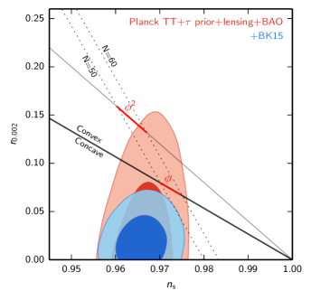
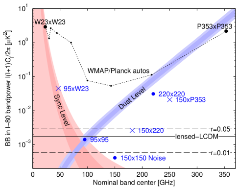
Fig. 6 shows the BK15 noise uncertainties in the $\ell\approx 80$ bandpowers as compared to the signal levels. Note that the new Keck 220 GHz band has approximately the same signal-to-noise on dust as Planck 353 GHz with two receiver-years of operation. In 2016 and 2017 we recorded an additional eight receiver-years of data which will reduce the noise by a factor of 5 & $\sqrt{5}$ for $220\times 220$ & $150\times 220$ respectively.

As seen in the lower right panel of Fig. 4 with four Keck receiver-years of data, our 95 GHz data starts to weakly prefer a non-zero value for the synchrotron amplitude for the first time. In 2017 alone BICEP3 recorded nearly twice as much data in the 95 GHz band as is included in the current result. We plan to proceed directly to a BK17 result which can be expected to improve substantially on the current results.

Figure 6: Expectation values and noise uncertainties for the $\ell\sim 80$ $BB$ bandpower in the BICEP2/Keck field. The solid and dashed black lines show the expected signal power of lensed-$\Lambda$CDM and $r_{0.05}=0.05$ & 0.01. Since CMB units are used, the levels corresponding to these are flat with frequency. The blue/red bands show the 1 and $2\sigma$ ranges of dust and synchrotron in the baseline analysis including the uncertainties in the amplitude and frequency spectral index parameters ($A_{\mathrm{sync,23}},\beta_{\mathrm{s}}$ and $A_{\mathrm{d,353}},\beta_{\mathrm{d}}$). The BICEP2/Keck auto-spectrum noise uncertainties are shown as large blue circles, and the noise uncertainties of the WMAP/Planck single-frequency spectra evaluated in the BICEP2/Keck field are shown in black. The blue crosses show the noise uncertainty of selected cross-spectra, and are plotted at horizontal positions such that they can be compared vertically with the dust and sync curves.

Dust decorrelation, and foreground complexity more generally, will remain a serious concern. With higher quality data we will be able to constrain the foreground behavior ever better, but of course we will also need to constrain it ever better. The BICEP Array experiment which is under construction will provide BICEP3 class receivers in the 30/40, 95, 150 and 220/270 GHz bands and is projected to reach $\sigma(r)<0.005$ within five years.

Appendix A Maps

Figures 7, 8 & 9 show the full sets of BK15 $T$/$Q$/$U$ maps at 95, 150 & 220 GHz. The right side of each figure shows realizations of noise created by randomly flipping the sign of data subsets while coadding the map—see Sec. V.B of Ref. BICEP2 Collaboration I (2014) for further details.

Figure 7: $T$, $Q$, $U$ maps at 95 GHz using data taken by two receivers of Keck Array during the 2014 & 2015 seasons—we refer to these maps as BK15₉₅. The left column shows the real data maps with $0.25^{\circ}$ pixelization as output by the reduction pipeline. The right column shows a noise realization made by randomly assigning positive and negative signs while coadding the data. These maps are filtered by the instrument beam (FWHM 43 arcmin Keck Array and BICEP2 Collaborations XI (shed)), timestream processing, and (for $Q$ & $U$) deprojection of beam systematics. Note that the horizontal/vertical and $45^{\circ}$ structures seen in the $Q$ and $U$ signal maps are expected for an $E$-mode dominated sky.

Figure 8: $T$, $Q$, $U$ maps at 150 GHz using all BICEP2/Keck data up to and including that taken during the 2015 observing season—we refer to these maps as BK15₁₅₀. These maps are directly analogous to the 95 GHz maps shown in Fig. 7 except that the instrument beam filtering is in this case 30 arcmin FWHM Keck Array and BICEP2 Collaborations XI (shed).

Figure 9: $T$, $Q$, $U$ maps at 220 GHz using data taken by two receivers of Keck Array during the 2015 season—we refer to these maps as BK15₂₂₀. These maps are directly analogous to the 95 GHz maps shown in Fig. 7 except that the instrument beam filtering is in this case 20 arcmin FWHM Keck Array and BICEP2 Collaborations XI (shed).

Appendix B 95 GHz and 220 GHz Internal Consistency Tests

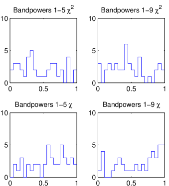
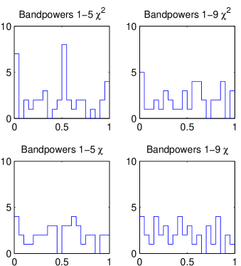
A powerful internal consistency test are data split difference tests which we refer to as “jackknives”. As well as the full coadd signal maps we also form many pairs of split maps where the splits are chosen such that one might expect different systematic contamination in the two halves of the split. The split halves are differenced and the power spectra taken. We then take the deviations of these from the mean of signal+noise simulations and form $\chi^{2}$ and $\chi$ (sum of deviations) statistics. In this section we perform tests of the 95 GHz and 220 GHz data sets which are exactly analogous to the tests of the 150 GHz data sets performed in Sec. VII.C of Ref. BICEP2 Collaboration I (2014) and Sec. 6.3 of Ref. Keck Array and BICEP2 Collaborations V (2015). (Since going from 8 to 9 receiver-years of Keck 150 GHz barely shifts the results we omit those tests for brevity.)

Tables B and B show the $\chi^{2}$ and $\chi$ statistics for the 95 GHz and 220 GHz jackknife tests respectively, while Figures 10 & 11 present the same results in graphical form. Note that these values are partially correlated—particularly the 1–5 and 1–9 versions of each statistic. We conclude that there is no evidence for corruption of the data at a level exceeding the noise.

Table 1: Jackknife PTE values from $\chi^{2}$ and $\chi$ (sum of deviations) tests for Keck Array 95 GHz data taken in 2014 and 2015. This table is analogous to Table I of Ref. Keck Array and BICEP2 Collaborations VI (2016) but extended to two seasons of data.

Jackknife	Band powers	Band powers	Band powers	Band powers
	1–5 $\chi^{2}$	1–9 $\chi^{2}$	1–5 $\chi$	1–9 $\chi$
Deck jackknife
EE	0.042	0.176	0.421	0.501
BB	0.132	0.186	0.852	0.952
EB	0.705	0.922	0.196	0.361
Scan Dir jackknife
EE	0.281	0.136	0.553	0.920
BB	0.154	0.100	0.980	0.968
EB	0.269	0.263	0.096	0.050
Tag Split jackknife
EE	0.194	0.377	0.743	0.930
BB	0.084	0.160	0.920	0.898
EB	0.685	0.870	0.259	0.319
Tile jackknife
EE	0.321	0.517	0.800	0.916
BB	0.862	0.978	0.832	0.792
EB	0.363	0.279	0.758	0.711
Phase jackknife
EE	0.858	0.800	0.627	0.621
BB	0.010	0.048	0.186	0.200
EB	0.337	0.423	0.721	0.758
Mux Col jackknife
EE	0.778	0.912	0.904	0.804
BB	0.651	0.497	0.419	0.880
EB	0.343	0.224	0.569	0.253
Alt Deck jackknife
EE	0.110	0.409	0.399	0.483
BB	0.335	0.487	0.569	0.677
EB	0.643	0.347	0.517	0.950
Mux Row jackknife
EE	0.459	0.557	0.599	0.896
BB	0.784	0.447	0.665	0.832
EB	0.697	0.621	0.132	0.042
Tile/Deck jackknife
EE	0.393	0.693	0.812	0.691
BB	0.267	0.309	0.303	0.333
EB	0.579	0.355	0.760	0.934
Focal Plane inner/outer jackknife
EE	0.617	0.419	0.906	0.992
BB	0.132	0.226	0.892	0.972
EB	0.984	0.629	0.683	0.806
Tile top/bottom jackknife
EE	0.595	0.020	0.593	0.407
BB	0.954	0.990	0.615	0.357
EB	0.289	0.505	0.954	0.840
Tile inner/outer jackknife
EE	0.305	0.605	0.158	0.090
BB	0.509	0.601	0.527	0.567
EB	0.449	0.447	0.375	0.096
Moon jackknife
EE	0.086	0.299	0.066	0.086
BB	0.900	0.852	0.291	0.325
EB	0.200	0.477	0.782	0.796
A/B offset best/worst
EE	0.090	0.034	0.766	0.295
BB	0.882	0.435	0.806	0.970
EB	0.613	0.902	0.611	0.561

Table 2: Jackknife PTE values from $\chi^{2}$ and $\chi$ (sum of deviations) tests for Keck Array 220 GHz data taken in 2015.

Jackknife	Band powers	Band powers	Band powers	Band powers
	1–5 $\chi^{2}$	1–9 $\chi^{2}$	1–5 $\chi$	1–9 $\chi$
Deck jackknife
EE	0.515	0.198	0.918	0.365
BB	0.024	0.028	0.008	0.178
EB	0.343	0.551	0.359	0.383
Scan Dir jackknife
EE	0.962	0.968	0.643	0.579
BB	0.154	0.261	0.579	0.754
EB	0.713	0.896	0.631	0.447
Tag Split jackknife
EE	0.030	0.014	0.715	0.976
BB	0.327	0.587	0.966	0.948
EB	0.483	0.840	0.234	0.431
Tile jackknife
EE	0.008	0.026	0.228	0.208
BB	0.242	0.469	0.846	0.850
EB	0.138	0.377	0.597	0.643
Phase jackknife
EE	0.549	0.858	0.966	0.928
BB	0.343	0.281	0.768	0.479
EB	0.447	0.271	0.669	0.727
Mux Col jackknife
EE	0.263	0.647	0.257	0.166
BB	0.567	0.693	0.116	0.257
EB	0.936	0.752	0.509	0.719
Alt Deck jackknife
EE	0.968	0.844	0.573	0.824
BB	0.030	0.172	0.409	0.539
EB	0.517	0.425	0.331	0.106
Mux Row jackknife
EE	0.695	0.611	0.166	0.094
BB	0.840	0.609	0.649	0.168
EB	0.509	0.311	0.605	0.347
Tile/Deck jackknife
EE	0.675	0.220	0.768	0.182
BB	0.968	0.990	0.681	0.834
EB	0.972	0.994	0.363	0.246
Focal Plane inner/outer jackknife
EE	0.020	0.038	0.010	0.016
BB	0.108	0.313	0.032	0.026
EB	0.012	0.040	0.509	0.433
Tile top/bottom jackknife
EE	0.210	0.108	0.076	0.028
BB	0.030	0.096	0.010	0.006
EB	0.709	0.581	0.685	0.549
Tile inner/outer jackknife
EE	0.503	0.637	0.503	0.828
BB	0.531	0.549	0.317	0.465
EB	0.477	0.471	0.826	0.723
Moon jackknife
EE	0.507	0.671	0.910	0.649
BB	0.942	0.894	0.281	0.267
EB	0.639	0.756	0.389	0.539
A/B offset best/worst
EE	0.561	0.854	0.066	0.082
BB	0.273	0.457	0.443	0.257
EB	0.531	0.569	0.425	0.441

Figure 10: Distributions of the jackknife $\chi^{2}$ and $\chi$ PTE values for the Keck Array 2014 & 2015 95 GHz data over the tests and spectra given in Table B. This figure is analogous to Fig. 12 of Ref. Keck Array and BICEP2 Collaborations VI (2016).

Figure 11: Distributions of the jackknife $\chi^{2}$ and $\chi$ PTE values for the Keck Array 2015 220 GHz data over the tests and spectra given in Table B.

Appendix C 95 GHz Spectral Stability

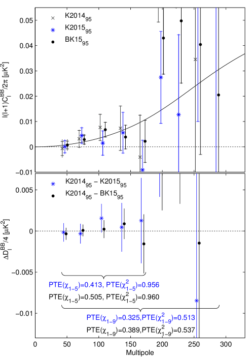
We next test the mutual compatibility of the 2014 and 2015 95 GHz spectra. We compare the differences of the real spectra to the differences of simulations which share the same underlying input skies. We perform the test in two ways: firstly by differencing the single season spectra (K2014₉₅ and K2015₉₅), and secondly by differencing the 2014 single season from the 2014+2015 season combined spectrum. Fig. 12 shows the results—the differences are seen to be consistent with noise fluctuation.

Figure 12: Upper: Comparison of the 95 GHz $BB$ auto-spectrum as previously published (K2014₉₅), for 2015 alone (K2015₉₅), and for the combination of the two (BK15₉₅). The inner error bars are the standard deviation of the lensed-$\Lambda$CDM+noise simulations, while the outer error bars include the additional fluctuation induced by the dust signal. Note that neither of these uncertainties are appropriate for comparison of the band power values—for this see the lower panel. (For clarity the sets of points are offset horizontally.) Lower: The difference of the pairs of spectra shown in the upper panel divided by a factor of four. The error bars are the standard deviation of the pairwise differences of signal+noise simulations which share common input skies (the simulations used to derive the outer error bars in the upper panel). Comparison of these points with null is an appropriate test of the compatibility of the spectra, and the PTE of $\chi$ and $\chi^{2}$ are shown. This figure is similar to Fig. 13 of Ref. Keck Array and BICEP2 Collaborations VI (2016).

Appendix D Additional Spectra

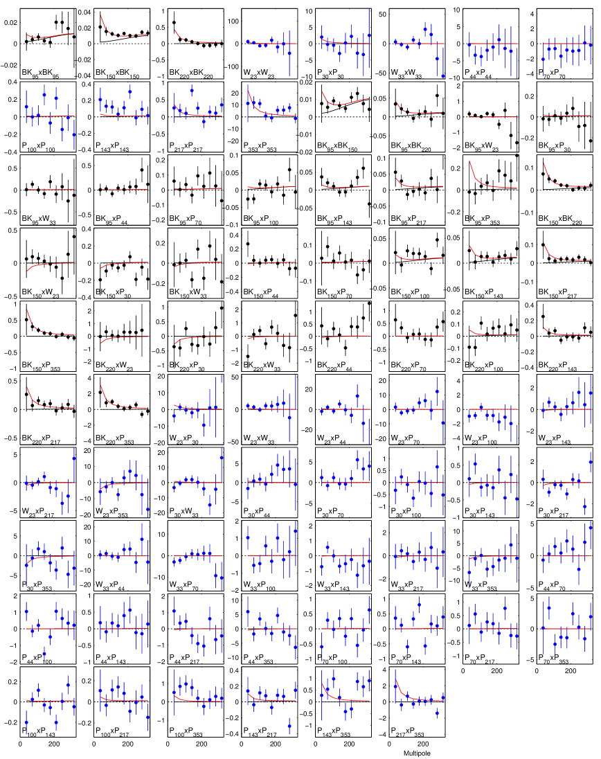
Fig. 2 shows only a small subset of the spectra which are used in the likelihood analysis and included in the COSMOMC input file. We are using three BICEP2/Keck bands, two WMAP bands, and seven Planck bands resulting in 12 auto- and 66 cross-spectra. In Fig. 13 we show all of these together with the maximum likelihood model from the baseline analysis whose parameters were quoted above. Most of the spectra not already shown in Fig. 2 have low signal-to-noise, although a few of them carry interesting additional information on the possible level of synchrotron as will be noted later.

The HL likelihood (Hamimeche and Lewis, 2008) we use for the primary analysis accounts for the full joint PDF of auto- and cross-spectral bandpowers which are derived from maps which are a combination of (correlated) signal and (mostly uncorrelated) noise. We choose to quantify the absolute goodness-of-fit of the data to the maximum likelihood model using a simple $\chi^{2}$ statistic which assumes that the bandpowers are normally distributed about their expectation values. We find that the distribution of this $\chi^{2}$ statistic for the standard (499) lensed-$\Lambda$CDM+dust+noise simulations versus their input model is significantly broader than the nominal theoretical distribution—presumably because of the non-normal distribution of the bandpowers. It is therefore most appropriate to compare the real data value to the simulated distribution.

For the $9\times 78=702$ bandpowers shown in Fig. 13, $\chi^{2}=(d-m)^{T}C^{-1}(d-m)=760$, where $d$ are the bandpower values, $m$ are the model expectation values, and $C$ is the bandpower covariance matrix. This has a nominal theory PTE of $0.06$ but a PTE versus the simulations of $0.19$. If instead we take the sum of the normalized deviations ($\sum{((d-m)/e)^{2}}$ where $e$ is the square-root of the diagonal of $C$) we find that the PTE versus the simulations is 0.23. We conclude that the parametric model which we have chosen—in combination with the approximation of Gaussian fluctuation of the dust (and synchrotron) sky patterns—is an adequate description of the presently available data.

Figure 13: The full set of $BB$ auto- and cross-spectra from which the joint model likelihood is derived. In all cases the quantity plotted is $100\ell C_{\ell}/2\pi$ ($\mu{\mathrm{K}^{2}}$). Spectra involving BICEP2/Keck data are shown as black points while those using only WMAP/Planck data are shown as blue points. The black lines show the expectation values for lensed-$\Lambda$CDM, while the red lines show the expectation values of the maximum likelihood lensed-$\Lambda$CDM+$r$+dust+synchrotron model ($r=0.020$, $A_{\mathrm{d,353}}=4.7$ $\mu{\mathrm{K}^{2}}$, $\beta_{\mathrm{d}}=1.6$, $\alpha_{\mathrm{d}}=-0.58$, $A_{\mathrm{sync,23}}=1.5$ $\mu{\mathrm{K}^{2}}$, $\beta_{\mathrm{s}}=-3.0$, $\alpha_{\mathrm{s}}=-0.27$, $\epsilon=-0.38$), and the error bars are scaled to that model.

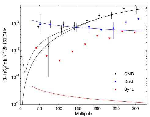
We also run a likelihood analysis to find the CMB and foreground contributions on a bandpower-by-bandpower basis. The baseline analysis is a single fit to all 9 bandpowers across 78 spectra with 8 parameters. Instead we now perform 9 separate fits—one for each bandpower—across the 78 spectra, with 6 parameters in each fit. These 6 parameters are the amplitudes of CMB, dust and synchrotron plus $\beta_{\mathrm{d}}$, $\beta_{\mathrm{s}}$ and $\epsilon$ with identical priors to the baseline analysis. The results are shown in Fig. 14—the resulting CMB values are consistent with lensed-$\Lambda$CDM while the dust values are consistent with the level of dust found in the baseline analysis. Synchrotron is tightly limited in all the multipole ranges, and not detected in any of them.

Figure 14: Spectral decomposition of the $BB$ data into synchrotron (red), CMB (black) and dust (blue) components at 150 GHz. The decomposition is calculated independently in each bandpower, marginalizing over $\beta_{\mathrm{d}}$, $\beta_{\mathrm{s}}$ and $\epsilon$ with the same priors as the baseline analysis. Error bars denote 68% credible intervals, with the point marking the most probable value. If the 68% interval includes zero, we also indicate the 95% upper limit with a downward triangle. (For clarity the sets of points are offset horizontally.) The solid black line shows lensed-$\Lambda$CDM with the dashed line adding on top an $r_{0.05}=0.02$ tensor contribution. The blue/red curves show sync/dust models consistent with the baseline analysis ($A_{\mathrm{d,353}}=4.6$ $\mu{\mathrm{K}^{2}}$, $\beta_{\mathrm{d}}=1.6$, $\alpha_{\mathrm{d}}=-0.4$ and $A_{\mathrm{sync,23}}=1.0$ $\mu{\mathrm{K}^{2}}$, $\beta_{\mathrm{s}}=-3.1$, $\alpha_{\mathrm{s}}=-0.6$ respectively).

Appendix E Likelihood Variation and Validation

E.1 Likelihood Evolution

We make only one model change versus the BK14 baseline analysis—we extend the range over which the sync/dust correlation parameter is marginalized from $0<\epsilon<1$ to the full possible range $-1<\epsilon<1$. This change was motivated by noting that the likelihood of this parameter peaked at zero in the BK14 analysis and following the philosophy of “allowing the data to select the model it prefers so long as this does not result in bias on $r$.” While we are not aware of any theoretical motivation to consider negative values, anti-correlation is presumably physically possible. Empirical evidence is sparse; Ref. Choi and Page (2015) reports a correlation of 0.2 for $30<\ell<200$, but the most recent Planck analysis detects (positive) sync/dust correlation only for $\ell<50$ Planck Collaboration 2018 XI (2018).

Fig. 15 shows the sequence of steps from the BK14 baseline analysis to the new baseline. Changing the $\epsilon$ marginalization range results in the change from green to magenta. Adding the 2015 data at 95 & 150 GHz causes the change from magenta to blue. Finally adding the new 220 GHz band results in the change from blue to black. The net result is a narrowing of the $r$ likelihood curve and a slight downward shift in the peak position. Note that we made the choice to change the $\epsilon$ prior based on the considerations above, and before looking at these real data results.

Figure 15: Evolution of the BK14 analysis to the “baseline” analysis as defined in this paper—see Appendix E.1 for details.

E.2 Likelihood Variation

Fig. 16 shows some variations from the baseline analysis choices. The HL likelihood (Hamimeche and Lewis, 2008) requires that one provide a “fiducial model”, but it is not supposed to matter very much what this model is so long as it is reasonably close to reality. Since the BKP paper we have used $A_{\mathrm{d,353}}=3.6$ $\mu{\mathrm{K}^{2}}$, $A_{\mathrm{sync}}=0$, $r=0$. Switching to $A_{\mathrm{d,353}}=5$ $\mu{\mathrm{K}^{2}}$, $A_{\mathrm{sync}}=0$, $r=0.05$ (blue) or $A_{\mathrm{d,353}}=5$ $\mu{\mathrm{K}^{2}}$, $A_{\mathrm{sync,23}}=2$ $\mu{\mathrm{K}^{2}}$, $r=0.05$ (red) makes little difference.

Figure 16: Likelihood results when varying the analysis choices—see Appendix E.2 for details.

Since BKP our baseline analysis has used a prior on the frequency spectral index of dust of $\beta_{\mathrm{d}}=1.59\pm 0.11$, using a Gaussian prior with the given $1\sigma$ width. These numbers are based on external information from Planck Planck Collaboration Int. XXII (2015); BICEP2/Keck and Planck Collaborations (2015) derived from other regions of the sky. In BK14 removing this prior resulted in a significant upshift in the $r$ constraint curve and a shift and broadening of the $A_{\mathrm{d}}$ curve. However, with the addition of the new Keck 220 GHz data we are now able to constrain $\beta_{\mathrm{d}}$ sufficiently well that changes when removing this prior are small (black to magenta). The $\beta_{\mathrm{d}}$ constraint curve (not shown) is close to Gaussian in shape with mean/$\sigma$ of 1.65/0.20. With further improvements in the data in the future we will no longer need the $\beta_{\mathrm{d}}$ prior and hence will be able to remove the uncertainty that comes from assuming that dust behavior in our sky patch is the same as the average behavior over larger regions of sky.

Our baseline prior on the frequency spectral index of synchrotron is $\beta_{\mathrm{s}}=-3.1\pm 0.3$ (Fuskeland et al., 2014), with a Gaussian shape with the given $1\sigma$ width. Relaxing to a uniform prior over the range $-4.5<\beta_{\mathrm{s}}<-2.0$ produces no significant changes (black to green). The data has little preference for the value of this parameter within the allowed range, which is not surprising since non-zero synchrotron amplitude is only weakly preferred.

Tightening the prior on the dust/sync correlation parameter from the baseline $-1<\epsilon<1$ to $\epsilon=0$ produces a small downshift in the $r$ constraint curve (black to cyan), as expected given what we already saw in Fig. 15. We show this case as we will invoke it when adding dust decorrelation to the model in Appendix F below. Putting a Gaussian prior on the dust/sync correlation with mean/$\sigma$ of 0.48/0.50 Planck Collaboration 2018 XI (2018) produces a smaller downshift in $r$ than setting $\epsilon=0$ (comparing yellow and cyan).

We explore the effect of uncertainty in the measured bandpasses for BICEP/Keck 95, 150 and 220 GHz channels. We expect such difference to be small and parameterize it as a fractional shift in the band center. We include one parameter for each frequency plus a correlated shift applied to all three channels. For each parameter, we use a Gaussian prior with mean/$\sigma$ of 0/0.02. These potential bandcenter shifts have little effect on the likelihood (black to dashed blue).

In the baseline analysis, the lensing amplitude is fixed to the $\Lambda$CDM expected value ($A_{\rm L}^{\rm BB}=1$). Relaxing this assumption we obtain the results shown in Fig. 17. With a unifrom prior, and marginalizing over all other parameters, we obtain $A_{\rm L}=1.15^{+0.16}_{-0.14}$. The zero-to-peak likelihood ratio is $1.3\times 10^{-17}$, and the probability to have a lower value is $5.8\times 10^{-19}$, which corresponds to a $8.8\sigma$ detection. This is the most significant detection of lensing using B-mode polarization to date. Due to the degeneracy between $r$ and $A_{\rm L}$, the $r$ likelihood curve shifts down. If we impose a prior from Planck, $A_{\rm L}=0.95\pm 0.04$ (Planck Collaboration 2015 XIII, 2016), the recovered $r$ likelihood curve is almost indistinguishable from the baseline case.

Figure 17: Likelihood results when allowing the lensing amplitude to be a free parameter—see Appendix E.2 for details.

Fig. 18 shows some variations of the data set selection. If we use the BICEP2/Keck data only (magenta) the $r$ constraint curve shifts down to peak at zero, while the $A_{\mathrm{d}}$ curve broadens slightly, and much larger values of $A_{\mathrm{sync}}$ become allowed. Bringing back WMAP (green) produces an even stronger downshift in $r$, and $A_{\mathrm{sync}}$ becomes better constrained. Switching LFI for WMAP (green to yellow) brings $r$ back up a bit and $A_{\mathrm{sync}}$ down (note the internal consistency problems of the LFI maps Planck Collaboration 2015 II (2016)). Adding HFI to BICEP/Keck+WMAP (green to red) brings $r$ up and leaves $A_{\mathrm{sync}}$ unchanged. BICEP/Keck+Planck (blue) has almost exactly the same $r$ curve as the baseline but a considerably wider $A_{\mathrm{sync}}$ curve. We can understand the behaviors in the $A_{\mathrm{sync}}$ curves, at least in part, by noting that in Fig. 13 the BK${}_{95}\times$W₂₃ bandpowers are positive while the BK${}_{95}\times$P₃₀ bandpowers are negative.

Figure 18: Likelihood results when varying the data set selection—see Appendix E.2 for details.

One additional variation which we explore is to include the $EE$ spectra (and hence also $EB$) in the fit under the assumption that $EE/BB=2$ for dust and synchrotron, as is shown to be close to the case in Refs Planck Collaboration 2018 XI (2018) and Krachmalnicoff et al. (2018). (While we have not included the $EE$ jackknife tests in this, or previous, papers they also produce distributions of $\chi$ and $\chi^{2}$ PTE values which are consistent with uniform.) As we can see in Fig. 2, $EE$ spectra such as BK${}_{220}\times$P₃₅₃ and P${}_{353}\times$P₃₅₃ certainly carry information on the amplitude of the dust emission and can presumably help indirectly to constrain $r$. In Fig. 18 adding $EE$ results in a small upshift in $r$ and significant tightening of the constraints on $A_{\mathrm{d}}$ and $A_{\mathrm{sync}}$. We will consider adding $EE$ to the baseline in future analyses, marginalizing over some range in the $EE/BB$ ratios.

At first glance it may appear surprising how large the shifts in the $r$ constraint are under the variations of the data selection shown in Fig. 18, and that many of the shifts are downward. However, when viewing the equivalent plots for the standard lensed-$\Lambda$CDM+dust+noise simulation realizations—which contain no tension between the data sets—the qualitative impression in many cases is similar. Note that while we verify in the next section that the baseline $r$ constraint is unbiased, we have not tested this for the data set variations explored here.

E.3 Likelihood Validation

The interpretation of $r$ likelihood curves such as the one shown in the upper left panel of Fig. 4 is not necessarily straightforward. Since the parameters are restricted to, and marginalized over, physical values only, biases can result. For instance, in a scenario where two parameters are fully degenerate, power will be assigned on average equally between them, and both will be biased low, with the curves for greater than 50% of realizations peaking at zero when the true values are zero. To investigate we make full COSMOMC runs on the ensemble of lensed-$\Lambda$CDM+dust+noise simulations. The left panel of Fig. 19 shows the resulting $r$ constraint curves, while the right panel shows that the CDF of the zero-to-peak likelihood ratios closely follows the simple analytic ansatz $\frac{1}{2}\left(1-f\left(-2\log{L_{0}/L_{\rm peak}}\right)\right)$ where $f$ is the $\chi^{2}$ CDF (for one degree of freedom). We find that 53% of the simulations peak at zero, and 19% have a lower zero-to-peak ratio than the real data—i.e. show more evidence for $r$ when the true value is in fact zero. This study provides powerful empirical evidence that the real data $r$ constraint curve can be taken at face value, provided the assumed foreground parameterization is an adequate description of reality.

Figure 19: Left: Likelihood curves for $r$ when running the baseline analysis on each of the lensed-$\Lambda$CDM+dust+noise simulations—half of them peak at zero. The real data curve is shown overplotted in heavy black. Right: The CDF of the zero-to-peak ratio (red) of the curves shown at right as compared to the simple analytic ansatz (solid black) $\frac{1}{2}\left(1-f\left(-2\log{L_{0}/L_{\rm peak}}\right)\right)$ where $f$ is the $\chi^{2}$ CDF (for one degree of freedom). About one fifth of the simulations offer more evidence for non-zero $r$ than the real data when the true value is actually zero (dashed black).

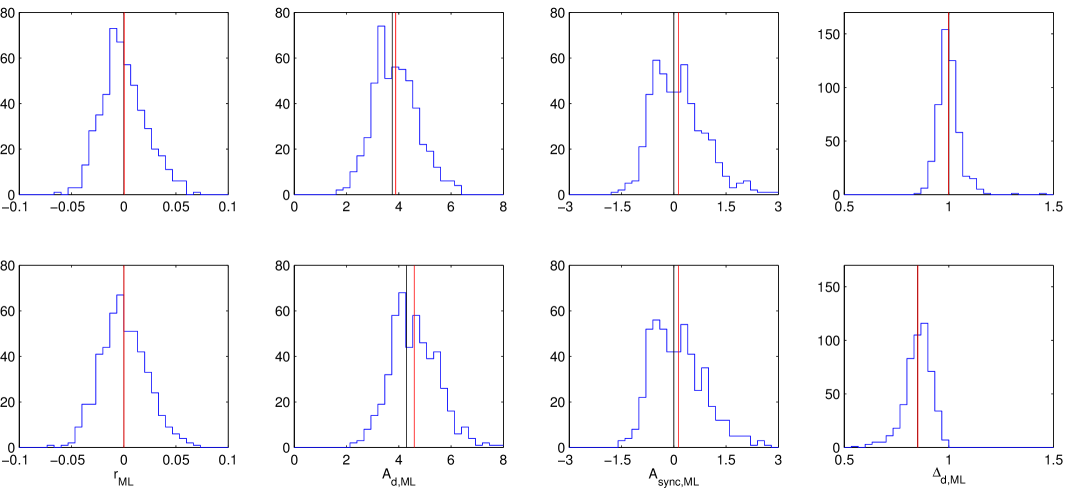
An alternate (and much faster) likelihood validation exercise is to run maximum likelihood searches, with non-physical parameter values allowed (such as negative $r$). When running on simulations generated according to the model being re-fit, we then have an a priori expectation that the input parameter values should be recovered in the mean. Fig. 20 shows the results when running on the standard lensed-$\Lambda$CDM+dust+noise simulations, with the same priors as for the baseline analysis—the input values are recovered in the mean. The first row of Table 3 summarizes: $\sigma(r)=0.020$, and bias in the mean value is small as compared to the noise. We prefer this $\sigma(r)$ measure of the intrinsic constraining power of the experiment since it is independent of the particular noise fluctuation that is present in the real data.

Figure 20: Results of a validation test running maximum likelihood search on simulations of a lensed-$\Lambda$CDM+dust+noise model with no synchrotron ($A_{\mathrm{d,353}}=3.75$ $\mu{\mathrm{K}^{2}}$, $\beta_{\mathrm{d}}=1.6$, $\alpha_{\mathrm{d}}=-0.4$, $A_{\mathrm{sync}}=0$). The baseline priors are applied on $\beta_{\mathrm{d}}$, $\beta_{\mathrm{s}}$, $\alpha_{\mathrm{d}}$, $\alpha_{\mathrm{s}}$ and $\epsilon$. The blue histograms are the recovered maximum likelihood values with the red lines marking their means and the black lines showing the input values. In the left panel $\sigma(r)=0.020$. See Appendix E.3 for details.

E.4 Exploration of Alternate Foreground Models

We now extend the maximum likelihood validation study to simulations using third-party foreground models. These models do not necessarily conform to our foreground parameterization and therefore when fit to it may potentially produce bias in $r$ at levels relevant compared to the noise. The second and subsequent rows of Table 3 summarize the results. The third-party models provide only a single realization of the foreground sky, and we add it on top of each of the lensed-$\Lambda$CDM+noise realizations that are used in the standard simulations.

Table 3: Uncertainty and bias on $r$ in simulations using Gaussian and 3rd party foreground models. (The numbers in parentheses suffer from disagreement between the priors and the model so bias is expected—see text for details.)

	$\overline{A_{d}}$	$\overline{A_{s}}$	$\sigma(r)$, $\overline{r}/\sigma(r)$
Model	($\mu{\mathrm{K}^{2}}$)	($\mu{\mathrm{K}^{2}}$)	$\beta_{\mathrm{d}}$ prior	$\beta_{\mathrm{d}}$ free	with decorr.
Gaussian	3.8	0.1	0.020, +0.1$\sigma$	0.023, 0.0$\sigma$	0.021, +0.0$\sigma$
PySM 1	10.9	1.1	0.026, +0.2$\sigma$	0.028, +0.2$\sigma$	0.028, +0.1$\sigma$
PySM 2	24.2	0.9	0.028, +0.1$\sigma$	0.029, +0.1$\sigma$	0.032, +0.1$\sigma$
PySM 3	12.1	1.1	(0.030, +0.4$\sigma$)	0.031, +0.1$\sigma$	(0.032, +0.2$\sigma$)
MHDv2	2.9	5.6	0.020, +0.2$\sigma$	0.027, –0.2$\sigma$	0.021, –0.1$\sigma$
G. Decorr.	4.6	0.1	(0.023, +1.5$\sigma$)	(0.026, +1.3$\sigma$)	0.022, +0.0$\sigma$

The PySM models 1, 2 and 3 are a1d1f1s1, a2d4f1s3 and a2d7f1s3 respectively, with the letters indicating AME (a), dust (d), free-free (f) & synchrotron (s), and the numbers referring to the various models of each as described in the PySM paper (Thorne et al., 2017). The a1 and f1 models are unpolarized and hence not relevant. The a2 model uses a Planck Commander Planck Collaboration 2015 X (2016) derived template and (dust) polarization angles together with a conservative 2% polarization fraction. No account for AME is made in our parametric model so this could potentially result in bias. The d1 model again uses Planck Commander derived templates for both the 353 GHz $Q/U$ patterns and the $T_{d}$ and $\beta_{\mathrm{d}}$ spectral parameters. The dust SED thus varies spatially, and this model therefore implements decorrelation of the dust pattern at some level (which in practice is found to be very small). Model d4 generalizes model d1 to the two temperature FDS model (Finkbeiner et al., 1999). Model d7 is a sophisticated physical model of dust grains as described in Ref. Hensley (2015) which does not necessarily conform to the modified blackbody SED. The s1 model takes the WMAP 23 GHz $Q/U$ maps and rescales them according to a power law using a spectral index map, and the s3 model adds on top of this a (spatially uniform) curvature of the synchrotron SED. The WMAP and Planck polarization templates are all noise dominated at smaller angular scales, so PySM filters out this noise and fills back in Gaussian realizations of foreground structure according to the recipe described in Sec. 3.1 of the PySM paper (Thorne et al., 2017).

We see in Table 3 that the PySM models predict considerably higher dust power in the BICEP/Keck field than is actually observed and that this pushes up $\sigma(r)$ somewhat as compared to the Gaussian results. The dust amplitude is sufficiently high in these models that $\beta_{\mathrm{d}}$ becomes well constrained for the noise levels and frequency range of the BK15 data—the prior on $\beta_{\mathrm{d}}$ can therefore be relaxed, and this is actually necessary for the PySM 3 model where the value of $\beta_{\mathrm{d}}$ preferred by the model is outside of the prior range, and bias on $r$ results if the prior is not relaxed.

The model labeled “MHDv2” is based on simulations of the Galactic magnetic field (Kritsuk et al., 2017) and naturally produces correlated dust and synchrotron emission. Since this model contains no explicit experimental data there is no noise issue, and the generated structure is non-Gaussian across the full range of $\ell$. This model gives a higher level of synchrotron than that which is preferred by the BICEP/Keck data ($A_{\mathrm{sync,23}}=5.6$ $\mu{\mathrm{K}^{2}}$ as compared to the maximum likelihood value of $1.5$ $\mu{\mathrm{K}^{2}}$ and 95% upper limit of $A_{\mathrm{sync,23}}<3.7$ $\mu{\mathrm{K}^{2}}$). This model also produces bias in the mean value of $r$ that is small compared to the noise level.

We conclude that none of the considered models produces relevant bias on $r$ when fitted to our foreground parameterization for the current experimental noise levels. These models span a variety of assumptions and methods and in some cases predict levels of foreground contamination much stronger than we actually observe in our field. However, there is no guarantee that the real foregrounds do not in fact produce greater bias than any of the considered models. We note that all of the above models produce dust decorrelation that is negligibly small compared to the current noise levels.

Appendix F Adding dust decorrelation

The simplest possible model of a given component of the polarized foreground emission (e.g. dust or synchrotron) is that it presents a fixed spatial pattern on the sky which scales with frequency according to a single SED. In this case the cross-spectrum between any two given frequencies is simply the geometric mean of the respective auto-spectra. In reality the morphology of the polarization pattern will inevitably vary as a function of frequency at some level. If $Q$ and $U$ at each given point on the sky deviate in sympathy away from the mean SED then the polarized intensity map will evolve as a function of frequency, but the polarization angles will remain constant. If $Q$ and $U$ deviate independently from the mean SED then both polarization intensity and angle will be functions of observing frequency. In either case the cross-spectra will be suppressed with respect to the geometric mean of the auto-spectra—a phenomenon which we refer to as decorrelation.

Planck Intermediate Paper XXX (Planck Collaboration Int. XXX, 2016) looked for suppression of the cross-spectral amplitudes in Figs. 6 & E.1 and did not find any evidence for decorrelation. However, that analysis was implicitly weighted towards lower $\ell$. Later Planck Intermediate Paper L (Planck Collaboration Int. L, 2017, hereafter PIPL) examined the cross-spectrum between 220 & 353 GHz as a function of $\ell$ and found evidence for a suppression effect which increased with $\ell$ and also when going to cleaner regions of sky (as determined by neutral hydrogen column density—see Fig. 3 of that paper). More recently, Ref. (Sheehy and Slosar, 2018) re-analyzed the now public Planck data and found no evidence for a detection of dust decorrelation. Finally the Planck team revisited the issue again in Planck Intermediate Paper LIV (Planck Collaboration 2018 XI, 2018, hereafter PIPLIV) and this time state that “We find no evidence for a loss of correlation.”

Decorrelation certainly exists at some level—the question is whether that level is relevant as compared to the current instrumental noise. To search for evidence of decorrelation in the BK15 data we add decorrelation of the dust pattern to our parametric model. We define the correlation ratio of the dust

$$\Delta_{\mathrm{d}}=\frac{\mathcal{D}_{80}(217\times 353)}{\sqrt{\mathcal{D}_{80}(217\times 217)\mathcal{D}_{80}(353\times 353)}},$$ (1)

where $\mathcal{D}_{80}$ is the dust power at $\ell=80$. This makes $\Delta_{\mathrm{d}}$ close to equivalent to $\mathcal{R}_{80}^{BB}$ as defined by PIPL and PIPLIV. We scale to other frequency combinations using the factor

$$f(\nu_{1},\nu_{2})=\frac{(\log(\nu_{1}/\nu_{2}))^{2}}{(\log(217/353))^{2}},$$ (2)

as suggested by PIPL.

Fig. 2 of PIPL suggests that decorrelation grows with increasing $\ell$, although in Sec. 4 they assume flat with $\ell$. In this paper we consider two possible scalings

$$g(\ell)=\left\{\begin{array}[]{ll}1&\,\text{flat case}\\ (\ell/80)&\,\text{linear case}\end{array}\right..$$ (3)

Since the $\ell$ range we are concerned with is not broad this choice turns out to make little practical difference.

The above scalings can produce extreme, and non-physical, behavior for widely separated frequencies and low/high $\ell$. We therefore re-map the nominal value using the following function

$$\Delta^{\prime}_{\mathrm{d}}(\nu_{1},\nu_{2},\ell)=\exp\left[\log(\Delta_{\mathrm{d}})\,f(\nu_{1},\nu_{2})\,g(\ell)\right],$$ (4)

such that $\Delta^{\prime}_{\mathrm{d}}$ remains in the range 0 to 1 for all values of $f$ and $g$. We note that for the frequency scaling this becomes the same as Eqn. 14 of Ref. (Vansyngel et al., 2017) which is shown in that paper to correspond to a Gaussian spatial variation in the foreground spectral index. (This is also used in PIPLIV.) For the moment we defer consideration of models which have both decorrelation of the dust pattern and correlation of the dust and synchrotron patterns simultaneously, setting $\epsilon=0$ whenever we allow $\Delta_{\mathrm{d}}\neq 1$. Note that in Fig. 16 we see that setting $\epsilon=0$ produces only small changes from the baseline analysis.

Fig. 2 shows the power spectra of the frequency bands which have the most power to constrain the dust contribution to the model. We can see visually that the (non-decorrelated) model from our previous BK14 analysis which is plotted there appears to be a good explanation of the observations (and in Appendix D it was shown formally that the new BK15 maximum likelihood model is compatible with the data). PIPL states that the mean neutral hydrogen column density in the BICEP2/Keck field is $\sim 1.6\times 10^{20}$ cm^-2 for which their Eqn. 6 gives a predicted correlation ratio value $\mathcal{R}_{50-160}^{BB}(217,353)=0.83$. To illustrate the effect of decorrelation in Fig. 2 we also re-plot the BK14 model modified with $\Delta_{\mathrm{d}}=0.85$ as the dashed red lines—this leaves the auto-spectra unchanged while suppressing the cross-spectra. The $150\times 353$ data appears to weakly disfavor the change while the $95\times 353$ weakly favors it. The above is simply for the purposes of illustration—we proceed below to include decorrelation and re-fit the model.

We expand the baseline likelihood analysis to include decorrelation and show results in Fig. 21. We consider several choices of prior on the $\Delta_{\mathrm{d}}$ parameter: i) Based on Table 1 of Ref. (Sheehy and Slosar, 2018) and Table 3 of Ref. Planck Collaboration 2018 XI (2018) we set a Gaussian prior with mean/$\sigma$ of 0.95/0.05 (truncated above 1), flat with $\ell$. ii) A Gaussian prior with mean/$\sigma$ of 1.00/0.05, linear with $\ell$. iii) A uniform prior 0 to 1, linear with $\ell$. All of these choices result in the $r$ likelihood curve shifting down and peaking at zero. However, note that introducing $\Delta_{\mathrm{d}}$ in a likelihood analysis which marginalizes only over the physically meaningful range $\Delta_{\mathrm{d}}\leq 1$ can result in a downward bias on $r$ even in the absence of a real decorrelation effect. For a given set of bandpowers it is possible to explain observed power in cross-spectra such as $150\times 353$ with a higher value of $A_{d}$ in combination with a lower value of $\Delta_{\mathrm{d}}$. The auto-spectra resist this preventing strong degeneracy, but a net bias still results. When we repeat the exercise of Fig. 19 running the full analysis on the standard lensed-$\Lambda$CDM+dust+noise simulations (which do not contain decorrelation), but include the decorrelation parameter in the analysis, we find that 72% of the $r$ curves peak at zero, and many of the $\Delta_{\mathrm{d}}$ curves peak below 1. We therefore choose not to include the decorrelation parameter in our baseline analysis at this time.

Figure 21: Likelihood results when allowing dust decorrelation—see Appendix F for details.

To check that the machinery remains unbiased when running maximum likelihood searches we repeat the exercise of Appendix E.3 but this time including the decorrelation parameter $\Delta_{\mathrm{d}}$ and allowing it to take values greater than one. To do this in a symmetrical manner we use

$$\Delta^{\prime}_{\mathrm{d}}(\nu_{1},\nu_{2},\ell)=2-\exp\left[\log(2-\Delta_{\mathrm{d}})\,f(\nu_{0},\nu_{1})\,g(\ell)\right].$$ (5)

In this exercise we take the linear $\ell$ scaling. Fig. 22 shows the results for the standard lensed-$\Lambda$CDM+dust+noise simulations which contain no decorrelation. We see that $\Delta_{\mathrm{d}}=1$ is recovered, and $r$ remains unbiased. We also show results for a toy highly decorrelated model which uses $\Delta_{\mathrm{d}}=0.85$ and linear scaling with $\ell$, following Eqns. 2–4. The input parameters of this model are also recovered in the mean. Finally we run the analysis with decorrelation on the third-party foreground models and give results for all the models in Table 3. As expected we see that the decorrelated simulations produce bias when re-analyzed without allowing decorrelation in the model.

Figure 22: Validation tests running the likelihood with the dust decorrelation parameter $\Delta_{\mathrm{d}}$ included. Upper row: Results for the same lensed-$\Lambda$CDM+dust+noise simulations shown in Fig. 20. Lower row: Results for the toy highly decorrelated dust model. The blue histograms are the recovered maximum likelihood values with the red lines marking their means and the black lines showing the input values. See Appendix F for details.

Running a maximum likelihood search including decorrelation on the real data we obtain $r_{0.05}=-0.012$, $A_{\mathrm{d,353}}=5.0$ $\mu{\mathrm{K}^{2}}$, $A_{\mathrm{sync,23}}=1.4$ $\mu{\mathrm{K}^{2}}$, $\beta_{\mathrm{d}}=1.6$, $\beta_{\mathrm{s}}=-3.1$, $\alpha_{\mathrm{d}}=-0.38$, $\alpha_{\mathrm{s}}=-0.52$, and $\Delta_{\mathrm{d}}=0.92$, i.e. $A_{\mathrm{d}}$ shifts up a bit, $r$ shifts down a bit, and $\Delta_{\mathrm{d}}$ is a little less than one. This model has a $\chi^{2}$ versus the data of 759 to be compared to the baseline model value of 760—the data shows little evidence for decorrelation of the dust pattern. As the data improves in the future the ability to constrain decorrelation while remaining unbiased on $r$ will improve.

Appendix G Definition of Multicomponent Model

The likelihood analysis uses a parametrized model to describe the bandpower expectation values as a combination of cosmological and foreground signals. The form of this model remains unchanged from BKP and BK14 except for the addition of foreground decorrelation (described in Appendix F). However, the choice of free parameters and priors has evolved over time due to improved BICEP/Keck data and new information from external sources. The previous papers describe the important features of the model but do not include a complete mathematical formulation, which we provide here.

Equation 6 describes contributions to the $BB$ cross-spectrum between maps at frequencies $\nu_{1}$ and $\nu_{2}$ (or auto-spectrum, if $\nu_{1}=\nu_{2}$) from dust, synchrotron, and the spatially-correlated component of dust and synchrotron. Parameter $A_{\mathrm{d}}$ specifies the dust power in units of $\mu\mathrm{K}_{\mathrm{\mbox{\tiny\sc cmb}}}^{2}$ at pivot frequency 353 GHz and angular scale $\ell=80$. Parameter $A_{\mathrm{sync}}$ specifies synchrotron power similarly, except with a pivot frequency of 23 GHz. The dust and synchrotron components scale as power laws in $\ell$ with slopes $\alpha_{\mathrm{d}}$ and $\alpha_{\mathrm{s}}$, respectively. Note that we define parameters $\alpha_{\mathrm{d}}$ and $\alpha_{\mathrm{s}}$ as the $\ell$ scaling of $\mathcal{D}_{\ell}\equiv\ell\left(\ell+1\right)C_{\ell}/2\pi$, not $C_{\ell}$ .

The level of spatial correlation between dust and synchrotron is set by parameter $\epsilon$. The correlated component scales with $\ell$ with a slope that is the average of $\alpha_{\mathrm{d}}$ and $\alpha_{\mathrm{s}}$, meaning that the correlation coefficient is assumed to be constant across all $\ell$.

Parameter $\Delta^{\prime}_{\mathrm{d}}$ accounts for decorrelation of the dust pattern between $\nu_{1}$ and $\nu_{2}$ and is defined in equation 4. Note that if $\nu_{1}=\nu_{2}$, then $\Delta^{\prime}_{\mathrm{d}}=1$ (perfect correlation). Parameter $\Delta^{\prime}_{\mathrm{s}}$ describes decorrelation of the synchrotron pattern but is not currently used. We currently do not include foreground decorrelation parameters in the dust–synchrotron correlated component. A complete foreground model would include the full set of correlations between dust and synchrotron fields at $\nu_{1}$ and the dust and synchrotron fields at $\nu_{2}$, but current data offer no guidance about the form of these correlations. For the time being, we consider dust decorrelation only as an extension to models with $\epsilon=0$, as noted in Appendix F.

Additional coefficients $f_{\mathrm{d}}$ and $f_{\mathrm{s}}$ capture the scaling of dust and synchrotron power from the pivot frequencies to the actual bandpasses of the maps labeled $\nu_{1}$ and $\nu_{2}$. This scaling includes the foreground SED as well as the conversion between $\mu{\mathrm{K}}_{\mathrm{\mbox{\tiny\sc cmb}}}$ units at the pivot frequency and at the target map bandpass. The SED model used for dust is a blackbody with temperature $T_{\mathrm{d}}=19.6\mathrm{K}$ multiplied by a power law with emissivity spectral index $\beta_{\mathrm{d}}$ Planck Collaboration Int. XXII (2015). The SED model used for synchrotron is a power law with spectral index $\beta_{\mathrm{s}}$ defined relative to a Rayleigh-Jeans spectrum. When integrating the SED and unit conversion factors over a map bandpass it is necessary to choose a bandpass convention. We define our bandpass functions to be proportional to the response as a function of frequency to a beam-filling source with uniform spectral radiance (the same convention as used by Planck Planck Collaboration IX (2014)).

$$\mathcal{D}_{\ell,BB}^{\nu_{1}\times\nu_{2}}=A_{\mathrm{d}}\Delta^{\prime}_{\mathrm{d}}f_{\mathrm{d}}^{\nu_{1}}f_{\mathrm{d}}^{\nu_{2}}\left(\frac{\ell}{80}\right)^{\alpha_{\mathrm{d}}}+A_{\mathrm{sync}}\Delta^{\prime}_{\mathrm{s}}f_{\mathrm{s}}^{\nu_{1}}f_{\mathrm{s}}^{\nu_{2}}\left(\frac{\ell}{80}\right)^{\alpha_{\mathrm{s}}}+\epsilon\sqrt{A_{\mathrm{d}}A_{\mathrm{sync}}}(f_{\mathrm{d}}^{\nu_{1}}f_{\mathrm{s}}^{\nu_{2}}+f_{\mathrm{s}}^{\nu_{1}}f_{\mathrm{d}}^{\nu_{2}})\left(\frac{\ell}{80}\right)^{(\alpha_{\mathrm{d}}+\alpha_{\mathrm{s}})/2}$$ (6)

The foreground contribution to $EE$ is similar, except that $A_{\mathrm{d}}$ and $A_{\mathrm{sync}}$ are scaled by the $EE/BB$ ratios for dust and synchrotron, respectively, which are both assumed to be equal to 2 Planck Collaboration 2018 XI (2018); Krachmalnicoff et al. (2018). The model for the $EB$ spectrum is zero, since neither CMB nor foreground signals are expected to break parity symmetry. We do not model the unpolarized foregrounds, nor include $TT/TE/TB$ spectra in the likelihood analysis.

Appendix H Summary of Simulations

We interpret the single realization of real data through comparison to several sets of simulations. With the exception of the alternate foreground models mentioned in Appendix E.4 above these have all been described and used in our previous papers BICEP2 Collaboration I (2014); BICEP2/Keck and Planck Collaborations (2015); Keck Array and BICEP2 Collaborations VI (2016).

We start by generating 499 pseudosimulations of noise by the sign-flip technique BICEP2 Collaboration I (2014); van Engelen et al. (2012). During the addition of multiple data subsets to form the final map we randomly flip the signs to cancel out sky signal. Each sequence is constructed to have equal weight in positives and negatives, and since the sequences are $>10^{4}$ in length the resulting noise realizations are found empirically to be uncorrelated. The mean spectra of these noise simulations are used to debias the real spectra (this being very important for the auto-spectra).

We also generate 499 realizations of lensed and unlensed $\Lambda$CDM by resampling timestream from simulated input maps and passing it through the full analysis pipeline (including filtering etc.) BICEP2 Collaboration I (2014). The unlensed simulations are useful to empirically determine the purity delivered by the matrix purification algorithm which is used to extract the $B$-mode signal in the presence of a much stronger $E$-mode.

From the simulated signal-cross-signal, noise-cross-noise and signal-cross-noise spectra we can construct the bandpower covariance matrix appropriate for any model containing a set of signal components with given SEDs BICEP2/Keck and Planck Collaborations (2015). When we do this we set to zero any term which has an expectation value of zero (under the assumption that signal and noise are uncorrelated) to reduce the Monte Carlo error in the resulting covariance matrix given the relatively modest number of realizations. We also set to zero the covariance between bandpowers that are separated by more than one bin in $\ell$, but, importantly, preserve the covariance between the the auto- and cross-spectra of the different frequency bands. This covariance matrix construction is used for the HL likelihood, and also to provide bandpower uncertainties shown, for example, in Fig. 13.

We also explicitly simulate simple dust input maps as power-law Gaussian realizations (with amplitude set to the observed dust amplitude in the BICEP/Keck patch) and pass these through the timestream sampling and pipeline re-mapping operation. They are then added to the lensed-LCDM and noise maps, and taken through to power spectra. We use these when it is important to match the fluctuations present in the real data in detail. One example is in the spectral stability tests shown in Fig. 12. Another example is when determining the PTE of the real data $\chi^{2}$ value in Appendix D.

Appendix I Lensing analysis

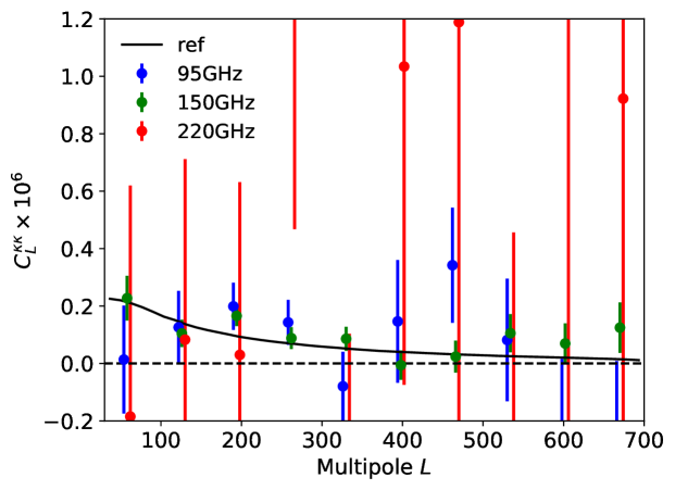
In Ref. Keck Array and BICEP2 Collaborations VIII (2016), we showed a detection of the gravitational lensing signal using the BK14 $E$- and $B$-modes at 150 GHz. We showed that the lensing signal is consistent with the standard $\Lambda$CDM model, and the BK14 $B$-mode spectrum at intermediate scales is dominated by lensing.

At 150 GHz, the sensitivity of BK15 to lensing is almost the same as that of BK14. Reconstructed lensing maps at 95 GHz and 220 GHz are still noisy. However, reconstructing lensing signals from BK15 data is important to test consistency of the data and simulation.

We reconstruct the lensing maps using BK15 data at 95 GHz, 150 GHz and 220 GHz based on the method described in Ref. Keck Array and BICEP2 Collaborations VIII (2016). Because the Planck lensing map has higher signal-to-noise than our reconstructed lensing maps, the BK15 lensing maps are then cross-correlated with the Planck lensing map provided by Ref. Ade et al. (2016). Fig. 23 shows the cross correlation of the reconstructed lensing signals between Planck and BK15 at each frequency. The amplitudes of the observed lensing spectra relative to the simulated spectra are found to be $A_{\rm L}^{\phi\phi}=1.24\pm 0.39$ (95 GHz), $1.14\pm 0.20$ (150 GHz) and $-1.13\pm 1.87$ (220 GHz), respectively. The data are consistent with our baseline simulation, and no spurious behavior is found in the lensing analysis.

Figure 23: Cross-correlation of the lensing reconstructions between Planck and BK15. We show the spectra for reconstruction using the BK15 95 GHz, 150 GHz and 220 GHz bands. The black solid line shows the theoretical lensing power spectrum.