Estimating menarcheal age distribution from partially recalled data

Abstract

In a cross-sectional study, adolescent and young adult females were asked to recall the time of menarche, if experienced. Some respondents recalled the date exactly, some recalled only the month or the year of the event, and some were unable to recall anything. We consider estimation of the menarcheal age distribution from this interval censored data. A complicated interplay between age-at-event and calendar time, together with the evident fact of memory fading with time, makes the censoring informative. We propose a model where the probabilities of various types of recall would depend on the time since menarche. For parametric estimation we model these probabilities using multinomial regression function. Establishing consistency and asymptotic normality of the parametric MLE requires a bit of tweaking of the standard asymptotic theory, as the data format varies from case to case. We also provide a non-parametric MLE, propose a computationally simpler approximation, and establish the consistency of both these estimators under mild conditions. We study the small sample performance of the parametric and non-parametric estimators through Monte Carlo simulations. Moreover, we provide a graphical check of the assumption of the multinomial model for the recall probabilities, which appears to hold for the menarcheal data set. Our analysis shows that the use of the partially recalled part of the data indeed leads to smaller confidence intervals of the survival function. Interval censoring, Informative censoring, Maximum likelihood estimation, Retrospective study, Current status data, Self consistency.

1 Introduction

In a recent survey conducted by the Indian Statistical Institute (ISI) in and around the city of Kolkata (Dasgupta, 2015), over four thousand randomly selected individuals, aged between 7 and 21 years, were sampled. In this retrospective and cross-sectional study, the subjects were interviewed on or around their birthdays. The data on female subjects contains age, menarcheal status, some physical measurements and information on some socioeconomic variables. If a subject had already experienced menarche, she was asked to recall the date of the onset of her menarche.

We considered a subset of the original data, consisting of respondents who came from a general caste family with monthly expenditure greater than or equal to Rs. 15000 and both parents graduate. Among the 289 females represented in the data set, 45 individuals did not have menarche, 68 individuals recalled the exact date of the onset of menarche, 43 and 30 individuals recalled the calendar month and the calendar year of the onset, respectively, and 103 individuals could not recall any range of dates. Thus, the data are interval-censored. A major goal of this study is to estimate the distribution of the age at onset of menarche.

This problem should be of interest to anyone working with incompletely recalled time-to-event data, of which there are many examples in the literature. The key variables in these studies include age at onset of menarche in adolescent and young adult females (Koo and Rohana, 1997), time-to-pregnancy (Joffe and others, 1995), time-to-weaning from breastfeeding (Gillespie and others, 2006), time-to-injury for victims injured during a year (Harel and others, 1994), time-to-employment (Mathiowetza and Ouncanb, 1988), and so on. In these studies, estimation of the time-to-event distribution is important for building a standard for individuals, comparing two populations or assessing the effect of a covariate. There is a possibility that the recalled time-to-event is inaccurate (Koo and Rohana, 1997; Mathiowetza and Ouncanb, 1988). In the ISI study, this problem was somewhat circumvented by allowing the respondents to report an interval in lieu of the exact age-at-menarche. The recalled intervals generally happened to be in terms of calendar months and years. We refer to this special type of incompleteness as partial recall.

Figure 1: Cumulative proportion of decreasing degrees of recall for different age ranges in menarcheal data

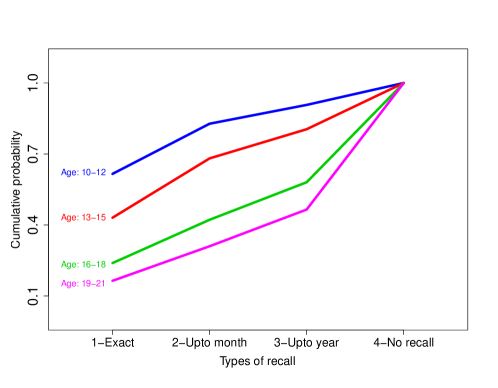
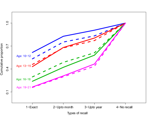
Figure 1 shows the cumulative proportions of successively less precise recall in different groups of ages at interview, for the respondents of the ISI study. It is seen that the lines do not cross and the age group order is preserved. Also, there is greater precision of recall at lower age group, i.e., memory fades with time. Thus, two subjects interviewed at the same age would have different chances of recalling their age at menarche, depending on which of them had experienced the event earlier. In other words, the censoring mechanism underlying such recall-based data is inherently informative. The natural question is: how can one model the different degrees of partial recall, so that the distribution of menarcheal age can be estimated?

There is no suitable model and method in the literature for estimating the time-to-event distribution from partially recalled data, though such data abound in various fields. Apart from the informative nature of censoring, the problem is complicated by the mismatch of the time scales of the partial recall information (expressed through calendar time) and the time-to-event (measured from a respondent-specific starting time, e.g., birth). Mirzaei and others (2015) and Mirzaei and Sengupta (2016) addressed the first issue by proposing a model for this type of informative censoring, but they bypassed the second issue by clubbing all the cases of partial recall with the cases of no recall.

In this paper we propose a realistic censoring model for estimating the time-to-event distribution from partially recalled data. We present our modelling framework in Section 2, and derive the appropriate likelihood under the proposed model. In Section 3 we express the likelihood as a product of densities in an appropriate space, and discuss asymptotic properties of a parametric maximum likelihood estimator (MLE). In Section 4 we derive the non-parametric maximum likelihood estimator (NPMLE) and an approximate MLE (AMLE), and also establish consistency of both these estimators. In Sections 5 and 6 we report the results of Monte Carlo simulations of small sample performance of the MLE and the AMLE, and present some diagnostic checks of adequacy of the model. We analyze the real data set in Section 7. We conclude with some discussion and indications of possible future extensions in Section 8. The proofs of all the theorems and the results of additional simulations and data analysis are given in the supplementary material.

2 Model and Likelihood

Consider a set of $n$ subjects having ages at occurrence of landmark events $T_{1},\ldots,T_{n}$, which are samples from the distribution $F$, with density $f$. Let these subjects be interviewed at ages $S_{1},\ldots,S_{n}$, respectively. Suppose the $S_{i}$s are samples from another distribution and are independent of the $T_{i}$s. Let $\delta_{i}$ be the indicator of $T_{i}\leq S_{i}$. This inequality means that the event for the $i$th subject had occurred on or before the time of interview.

In the case of current status data, one only observes $(S_{i},\delta_{i}),i=1,2,\ldots,n$. The corresponding likelihood, conditional on the times of interview, is

$$\prod_{i=1}^{n}[F(S_{i})]^{\delta_{i}}[\bar{F}(S_{i})]^{1-\delta_{i}},$$ (1)

where $\bar{F}(S_{i})=1-F(S_{i})$. For properties of the MLE based on the above likelihood, see Lee and Wang (2003).

The structure of recalled data is generally more complicated. Mirzaei and others (2015) proposed a simplistic model, where the subject may either recall the time of the event exactly or not remember it at all. They used an indicator, $\varepsilon_{i}$, to record whether an exact recall is possible. As the chance of recall may depend on the time elapsed since the event, they modeled the non-recall probability as a function of this time. According to this model,

$$P(\varepsilon_{i}=0|S_{i}=s,T_{i}=t)=\pi(s-t)\qquad\mbox{for}\quad 0<t<s,$$

for some non-recall probability function $\pi$. Thus, the likelihood is

$$\prod_{i=1}^{n}\left[\left(\int_{0}^{S_{i}}f(u)\pi(S_{i}-u)du\right)^{1-\varepsilon_{i}}\left[f(T_{i})(1-\pi(S_{i}-T_{i}))\right]^{\varepsilon_{i}}\right]^{\delta_{i}}[\bar{F}(S_{i})]^{1-\delta_{i}}.$$ (2)

Let us now consider the possibility that the $i$th subject can recall the date of the event only up to a calendar month or a calendar year, and define the recall status variable $\varepsilon_{i}$ for the $i$th subject as

$$\varepsilon_{i}=\left\{\begin{array}[]{ll}0&\text{if there is exact recall},\\ 1&\text{if the date is recalled up to the calendar month},\\ 2&\text{if the date is recalled up to the calendar year},\\ 3&\text{if the date is not recalled}.\end{array}\right.$$ (3)

The value of $\varepsilon_{i}$ concerns the state of recall. When $\delta_{i}=1$, $\varepsilon_{i}=0$ means that the exact date of the event is recalled. When $\delta_{i}=0$, $\varepsilon_{i}$ may be assigned the value 0, as no recall failure is expected in case the event is reported not to have happened.

We regard the four scenarios as outcomes of a multinomial selection, where allocation probabilities depend on the time elapsed since the occurrence of the event. Thus, for $0<t<s$, we model the allocation probabilities as

$$\begin{array}[]{l}P(\varepsilon_{i}=0|S_{i}=s,T_{i}=t)=\pi^{(0)}(s-t),\\ P(\varepsilon_{i}=1|S_{i}=s,T_{i}=t)=\pi^{(1)}(s-t),\\ P(\varepsilon_{i}=2|S_{i}=s,T_{i}=t)=\pi^{(2)}(s-t),\\ P(\varepsilon_{i}=3|S_{i}=s,T_{i}=t)=\pi^{(3)}(s-t).\end{array}$$ (4)

where $\sum_{k=0}^{3}\pi^{(k)}(s-t)=1$.

We refer to the set-up described in the first paragraph of this section, together with (3) and (4) as the proposed model. According to this model, contributions to the likelihood in different cases are as follows.

Case

(i) When $\delta_{i}=0$ (the event has not occurred till the time of observation), the contribution of the $i$th individual to the likelihood is $\bar{F}(S_{i})$.

Case

(ii): When $\delta_{i}=1$ and $\varepsilon_{i}=0$ (the event has occurred and the $i$th individual can remember the time), the contribution of the individual to the likelihood is $f(T_{i})\pi^{(0)}(S_{i}-T_{i})$.

Case

(iii): When $\delta_{i}=1$ and $\varepsilon_{i}=1$ (the event has occurred but the $i$th individual can only recall the calendar month of the event), the contribution of the individual to the likelihood is $\int_{M_{i1}}^{M_{i2}}f(u)\pi^{(1)}(S_{i}-u)du$, where $M_{i1}$ and $M_{i2}$ are the ages of the individual at the beginning and the end of the calendar month recalled by the individual.

Case

(iv): When $\delta_{i}=1$ and $\varepsilon_{i}=2$ (the event has occurred but the $i$th individual can only recall the calendar year of the event), the contribution of the individual to the likelihood is $\int_{Y_{i1}}^{Y_{i2}}f(u)\pi^{(2)}(S_{i}-u)du$, where $Y_{i1}$ and $Y_{i2}$ are the ages of the individual at the beginning and the end of the calendar year recalled by the individual.

Case

(v): When $\delta_{i}=1$ and $\varepsilon_{i}=3$ (the event has occurred but the $i$th individual cannot recall the time at all), the contribution of the individual to the likelihood is $\int_{0}^{S_{i}}f(u)\pi^{(3)}(S_{i}-u)du$.

Therefore, the overall likelihood is

$$\prod_{i=1}^{n}[\bar{F}(S_{i})] {}^{1-\delta_{i}}\Biggl{[}\left(f(T_{i})\pi^{(0)}(S_{i}-T_{i})\right)^{I_{(\varepsilon_{i}=0)}}\left(\int_{M_{i1}}^{M_{i2}}f(u)\pi^{(1)}(S_{i}-u)du\right)^{I_{(\varepsilon_{i}=1)}}\times$$

$$\left(\int_{Y_{i1}}^{Y_{i2}}f(u)\pi^{(2)}(S_{i}-u)du\right)^{I_{(\varepsilon_{i}=2)}}\left(\int_{0}^{S_{i}}f(u)\pi^{(3)}(S_{i}-u)du\right)^{I_{(\varepsilon_{i}=3)}}\Biggr{]}^{\delta_{i}}.$$ (5)

Note that when $\pi^{(1)}=\pi^{(2)}=0$, the likelihood (5) reduces to (2). When $\pi^{(1)}=\pi^{(2)}=0$ and $\pi^{(0)}$ is a constant, it becomes a constant multiple of the likelihood corresponding to non-informatively interval censored data. If $\pi^{(0)}=\pi^{(1)}=\pi^{(2)}=0$, it reduces to the current status likelihood (1).

While the proposed model is specific to the data at hand, it can easily be adjusted for arbitrary types of recall, which need not even be ordered.

The factors in the product likelihood (5) have different forms in different cases. We now show that they can be expressed as the common density of some random vector with respect to a suitable dominating measure.

The main challenge to obtaining a common format of the data lies in the fact that $M_{i1}$, $M_{i2}$, $Y_{i1}$ and $Y_{i2}$ are the ages of the $i$th individual at specified calendar times. We make use of the fact that these observables are functions of $T_{i}$ and the date of birth of the $i$th individual. Specifically, for the $i$th subject, let $m_{i}$ be the serial number of the month of birth within the year of birth and $d_{i}$ be the time (measured in years) from the beginning of the month of birth till the event of birth. For the sake of simplicity, we assume that every year has duration $1$ and every month has duration $1/12$.

When $\epsilon_{i}=1$, i.e., the month of the event is recalled, we write

$$\begin{array}[]{l}M_{i1}=\lfloor 12(d_{i}+T_{i})\rfloor/12-d_{i},\\ M_{i2}=M_{i1}+1/12,\end{array}$$ (6)

where $\lfloor\cdot\rfloor$ is the integer part of its argument. Thus, the variables $\lfloor 12(d_{i}+T_{i})\rfloor$, $m_{i}$ and $d_{i}$ can be obtained from $M_{i1}$, $M_{i2}$, $m_{i}$ and $d_{i}$ and vice versa. Likewise, when $\epsilon_{i}=2$, i.e., the year of the event is recalled, we write

$$\begin{array}[]{l}Y_{i1}=\lfloor\big{(}T_{i}+d_{i}+(m_{i}-1)/12\big{)}\rfloor-\big{(}d_{i}+(m_{i}-1)/12\big{)},\\ Y_{i2}=Y_{i1}+1.\end{array}$$ (7)

It is clear that the variables $\lfloor\big{(}T_{i}+d_{i}+(m_{i}-1)/12\big{)}\rfloor$, $m_{i}$ and $d_{i}$ are equivalent to $Y_{i1}$, $Y_{i2}$, $m_{i}$ and $d_{i}$. Therefore, we define the variable

$$V_{i}=\left\{\begin{array}[]{ll}T_{i}&\text{if $\varepsilon_{i}=0$ , $\delta_{i}=1$,}\\ \lfloor 12(d_{i}+T_{i})\rfloor/12&\text{if $\varepsilon_{i}=1$ , $\delta_{i}=1$,}\\ \lfloor\big{(}T_{i}+d_{i}+(m_{i}-1)/12\big{)}\rfloor&\text{if $\varepsilon_{i}=2$ , $\delta_{i}=1$,}\\ 0&\text{if $\varepsilon_{i}=3$, $\delta_{i}=1$, or if $\delta_{i}=0$,}\end{array}\right.$$ (8)

which captures the essential part of the occasionally observable variables $T_{i}$, $M_{i1}$, $M_{i2}$, $Y_{i1}$ and $Y_{i2}$, and subsequently work with the observable vector

$$Y_{i}=(S_{i},V_{i},\varepsilon_{i},\delta_{i},m_{i},d_{i}).$$ (9)

We have already assumed that the $T_{i}$s (time-to-event) are samples from the distribution $F$ and the $S_{i}$s (ages on interview date) are samples from another distribution. We now denote by $G_{1}$, $G_{2}$ and $G_{3}$ the distributions of $S_{i}$, $m_{i}$ and $d_{i}$, respectively, for every $i$. The distribution $G_{2}$ is defined over the set $\{1,2,\ldots,12\}$, and $G_{3}$ is defined over the interval $[0,1/12]$. The latter assumption disregards the fact that $d_{i}$ is known only up to days (measured as fixed fractions of a year), to keep the description simple.

Theorem 2.1 presented below gives the density of $Y_{i}$, after the subscript $i$ is dropped for simplicity. The dominating probability measure used for defining this density is $\mu=\vartheta_{1}\times\vartheta_{2}\times\vartheta_{3}\times\vartheta_{4}\times\vartheta_{5}\times\vartheta_{6}$ where $\vartheta_{1}$ is the measure with respect to which $G_{1}$ has a density (e.g., the counting or the Lebesgue measure, depending on whether $G_{1}$ is discrete or continuous), $\vartheta_{2}$ is the sum of the counting and the Lebesgue measures, each of $\vartheta_{3},\vartheta_{4}$ and $\vartheta_{5}$ is the counting measure and $\vartheta_{6}$ is the Lebesgue measure (Ash, 2000).

Theorem 2.1.

The density of $Y=(S,V,\varepsilon,\delta,m,d)$ with respect to the measure $\mu$ is

$$\hskip-25.0pth(s,v,\varepsilon,\delta,m,d)$$ (15)

$$= \left\{\begin{array}[]{ll}g_{1}(s)g_{2}(m)g_{3}(d)\bar{F}(s)&\text{if $\delta=0$},\\ g_{1}(s)g_{2}(m)g_{3}(d)f(v)\pi^{(0)}(s-v)I_{(v<s)}&\text{if $\varepsilon=0$ and $\delta=1$},\\ g_{1}(s)g_{2}(m)g_{3}(d)\int_{v-d}^{min(s,v+\frac{1}{12}-d}f(u)\pi^{(1))}(s-u)du&\text{if $\varepsilon=1$ and $\delta=1$},\\ g_{1}(s)g_{2}(m)g_{3}(d)\int_{v-d-\frac{m-1}{12}}^{min(s,v+1-d-\frac{m-1}{12})}f(u)\pi^{(2)}(s-u)du&\text{if $\varepsilon=2$ and $\delta=1$},\\ g_{1}(s)g_{2}(m)g_{3}(d)\int_{0}^{s}f(u)\pi^{(3)}(s-u)du&\text{if $\varepsilon=3$ and $\delta=1$},\end{array}\right.$$

where $g_{1}$, $g_{2}$ and $g_{3}$ are the densities of $G_{1}$, $G_{2}$ and $G_{3}$ with respect to the measures $\vartheta_{1}$, $\vartheta_{5}$ and $\vartheta_{6}$, respectively.

Theorem 2.1 implies that the likelihood (5) can be written as

$$\prod_{i=1}^{n}[\bar{F}(S_{i})]^{1-\delta_{i}}\Biggl{[}\left(f(V_{i})\pi^{(0)}(S_{i}\!-\!V_{i})\right)^{I_{(\varepsilon_{i}=0)}}\!\left(\int_{V_{i}-d_{i}}^{V_{i}-d_{i}+\frac{1}{12}}\!\!f(u)\pi^{(1)}(S_{i}\!-\!u)du\!\right)^{I_{(\varepsilon_{i}=1)}}$$

$$\times\!\left(\int_{V_{i}-d_{i}-\frac{m_{i}-1}{12}}^{V_{i}-d_{i}-\frac{m_{i}-1}{12}+1}\!\!f(u)\pi^{(2)}(S_{i}\!-\!u)du\!\right)^{I_{(\varepsilon_{i}=2)}}\!\!\!\left(\int_{0}^{S_{i}}\!\!f(u)\pi^{(3)}(S_{i}\!-\!u)du\!\right)^{I_{(\varepsilon_{i}=3)}}\Biggr{]}^{\delta_{i}}\!\!,$$

$$\qquad\qquad=\frac{\prod_{i=1}^{n}h(S_{i},V_{i},\varepsilon_{i},\delta_{i},m_{i},d_{i})}{\prod_{i=1}^{n}g_{1}(S_{i})g_{2}(m_{i})g_{3}(d_{i})},$$ (16)

where the $i$th factor is the conditional density of $(V_{i},\varepsilon_{i},\delta_{i})$ given $(S_{i},m_{i},d_{i})$.

3 Parametric estimation

Suppose the forms of the functions $\bar{F}$, $f$, $\pi^{(0)}$, $\pi^{(1)}$, $\pi^{(2)}$ and $\pi^{(3)}$ in the likelihood (5) are known up to a few parameters, and accordingly they are written as $\bar{F}_{\theta}$, $f_{\theta}$, $\pi^{(0)}_{\eta}$, $\pi^{(1)}_{\eta}$, $\pi^{(2)}_{\eta}$ and $\pi^{(3)}_{\eta}$, respectively. The MLE of the (possibly vector) parameters $\theta$ and $\eta$ are obtained by maximizing (5).

Since the equivalent likelihood (16) is identified as a product of conditional densities, standard results for consistency and asymptotic normality of the MLE become applicable. The regularity conditions for these results would then be specified in terms of the density of $Y_{i}$. In the first section of the supplementary material, we provide easily verifiable sufficient conditions that involve the density $f_{\theta}$ (the density of $T_{i}$) and the functions $\pi_{\eta}^{(0)},\pi_{\eta}^{(1)},\pi_{\eta}^{(2)}$ and $\pi_{\eta}^{(3)}$, which define the conditional probability distribution of the random variable $\varepsilon_{i}$ given $T_{i}$ and $S_{i}$.

4 Non-parametric estimation

4.1 Non-parametric MLE

Before embarking on the task of estimation, we establish the following result on the issue of identifiability.

Theorem 4.1.

The distribution functions $G_{1}$ and $F$, and recall probabilities $\pi^{(k)}$, $k=0,1,2,3$ are identifiable from $h$ in (15).

The likelihood (5) is difficult to maximize because of the integrals contained in the expression. In order to simplify it, we assume that the function $\pi^{(l)}$ in (5) is piecewise constant, having the form $\pi^{(l)}(x)=b_{l1}I(x_{1}<x\leq x_{2})+b_{l2}I(x_{2}<x\leq x_{3})+\ldots+b_{lL}I(x_{L}<x<\infty)$, $l=0,1,2,3$, where $0=x_{1}<x_{2}<\cdots<x_{L}$ are a chosen set of time-points and $b_{l1},b_{l2},\ldots,b_{lL}$ are unspecified parameters taking values in the range $[0,1]$ such that $\sum_{l=0}^{3}b_{lj}=1$ for $j=1,2,\ldots,L$. Then the likelihood (5) reduces to

$$L= \prod_{i=1}^{n}[\bar{F}(S_{i})]^{1-\delta_{i}}\Biggl{[}\left\{f(T_{i})\left(\sum_{l=1}^{L}b_{0l}I\big{(}W_{l+1}(S_{i})<T_{i}\leq W_{l}(S_{i})\big{)}\right)\right\}^{I_{(\varepsilon_{i}=0)}}$$

$$\hskip-20.0pt\times\!\left\{\sum_{\begin{subarray}{c}l=1\\ [W_{l+1}(S_{i}),W_{l}(S_{i})]\cap[M_{i1},M_{i2}]\neq\phi\end{subarray}}^{L}b_{1l}\Big{(}F\big{(}\min(W_{l}(S_{i}),M_{i2})\big{)}\!-\!F\big{(}\max(W_{l+1}(S_{i}),M_{i1})\big{)}\Big{)}\right\}^{I_{(\varepsilon_{i}=1)}}$$

$$\hskip-20.0pt\times\!\left\{\sum_{\begin{subarray}{c}l=1\\ [W_{l+1}(S_{i}),W_{l}(S_{i})]\cap[Y_{i1},Y_{i2}]\neq\phi\end{subarray}}^{L}b_{2l}\Big{(}F\big{(}\min(W_{l}(S_{i}),Y_{i2})\big{)}\!-\!F\big{(}\max(W_{l+1}(S_{i}),Y_{i1})\big{)}\Big{)}\right\}^{I_{(\varepsilon_{i}=2)}}$$

$$\hskip-20.0pt\times\!\left\{\sum_{l=1}^{L}b_{3l}\Big{(}F(W_{l}(S_{i}))-F(W_{l+1}(S_{i}))\Big{)}\right\}^{I_{(\varepsilon_{i}=3)}}\Biggr{]}^{\delta_{i}},$$ (17)

where $W_{l}(S_{i})=(S_{i}-x_{l})\vee t_{min}$ for $l=1,\ldots,L$ and $W_{L+1}(S_{i})=t_{min},i=1,2,\ldots,n$. The likelihood (17) involves probabilities assigned to intervals of the type $[t,t_{max}]$ or $(t,t_{max}]$, as per the baseline probability distribution. Since these intervals have overlap, we try to write them as unions of some disjoint intervals. Let ${\cal I}_{1}$, ${\cal I}_{2}$, ${\cal I}_{3}$, ${\cal I}_{4}$ and ${\cal I}_{5}$ be sets of indices $i$ (between 1 and $n$) that satisfy the conditions $\delta_{i}=0$, $\delta_{i}\varepsilon_{i}=1$, $\delta_{i}(1-\varepsilon_{i})=1$, $\delta_{i}\varepsilon_{i}=2$ and $\delta_{i}\varepsilon_{i}=3$. respectively. Consider the intervals

$$\begin{array}[]{r@{\hskip 3pt}c@{\hskip 3pt}ll}A_{i}\hskip 3.0&=\hfil\hskip 3.0&(S_{i},t_{max}]&\mbox{for }i\in{\cal I}_{1},\\[1.72218pt] A_{i}\hskip 3.0&=\hfil\hskip 3.0&[T_{i},t_{max}]&\mbox{for }i\in{\cal I}_{2},\\[1.72218pt] A_{i}^{\prime}\hskip 3.0&=\hfil\hskip 3.0&(T_{i},t_{max}]&\mbox{for }i\in{\cal I}_{2},\\[2.15277pt] A_{il}\hskip 3.0&=\hfil\hskip 3.0&\left\{\begin{matrix}(W_{l}(S_{i}),t_{max}],&l=1,\ldots,L,\\ [W_{l}(S_{i}),t_{max}],&l=k+1,\ \ \ \,\\ \end{matrix}\right.&\mbox{for}\ i\in{\cal I}_{2}\cup{\cal I}_{3},\\[8.61108pt] B_{il}\hskip 3.0&=\hfil\hskip 3.0&[W_{l+1}(S_{i})\vee M_{i1},W_{l+1}(S_{i})\wedge M_{i1}]&\mbox{for }i\in{\cal I}_{4}\ \&\ l=1,\ldots,L,\\[1.72218pt] C_{il}\hskip 3.0&=\hfil\hskip 3.0&[W_{l+1}(S_{i})\vee Y_{i1},W_{l+1}(S_{i})\wedge Y_{i1}]&\mbox{for }i\in{\cal I}_{5}\ \&\ l=1,\ldots,L,\\ \end{array}$$ (18)

and the sets

$$\begin{array}[]{r@{\hskip 3pt}c@{\hskip 3pt}l}{\cal A}_{1}\hskip 3.0&=\hfil\hskip 3.0&\{A_{i}:\ \ i\in{\cal I}_{1}\},\\[1.07639pt] {\cal A}_{2}\hskip 3.0&=\hfil\hskip 3.0&\{A_{i}\setminus A_{i}^{\prime}:\ \ i\in{\cal I}_{2}\},\\[1.07639pt] {\cal A}_{3}\hskip 3.0&=\hfil\hskip 3.0&\{A_{i}^{\prime}:\ \ i\in{\cal I}_{2}\},\\[1.07639pt] {\cal A}_{4}\hskip 3.0&=\hfil\hskip 3.0&\{A_{i(l+1)}\setminus A_{il}:\ \ 1\leq l\leq L\mbox{ and}\ i\in{\cal I}_{3}\},\\[1.07639pt] {\cal A}_{5}\hskip 3.0&=\hfil\hskip 3.0&\{B_{il}:\ \ 1\leq l\leq L\mbox{ and}\ i\in{\cal I}_{4}\},\\[1.07639pt] {\cal A}_{6}\hskip 3.0&=\hfil\hskip 3.0&\{C_{il}:\ \ 1\leq l\leq L\mbox{ and}\ i\in{\cal I}_{5}\}.\\ \end{array}$$ (19)

As $F$ is absolutely continuous, the elements of ${\cal A}_{2}$ and ${\cal A}_{3}$ are distinct with probability 1. Let $n_{i}$ be the cardinality of ${\cal I}_{i}$, $i=1,2,3,4,5$. We arrange the singleton elements of ${\cal A}_{2}$ in increasing order, and denote them as $B_{1},B_{2},\ldots,B_{n_{2}}$. We also arrange the elements of ${\cal A}_{3}$ in the corresponding order and denote them as $B_{n_{2}+1},B_{n_{2}+2},\ldots,B_{2n_{2}}$. We then collect the unique elements of ${\cal A}_{1}\cup{\cal A}_{4}\cup{\cal A}_{5}\cup{\cal A}_{6}$ that are distinct from $B_{1},B_{2},\ldots,B_{2n_{2}}$, and denote them as $B_{2n_{2}+1},B_{2n_{2}+2},\ldots,B_{M}$. Observe that the collection $B_{1},B_{2},\ldots,B_{M}$ consists of the distinct elements of $\bigcup_{i=1}^{6}{\cal A}_{i}$, arranged in a particular order. Denote the non-empty subsets of the index set $\{1,2,\ldots,M\}$ by $s_{1},s_{2},\ldots,s_{2^{M}-1}$. Define

$$I_{r}=\left\{\bigcap_{i\in s_{r}}B_{i}\right\}\bigcap\left\{\bigcap_{i\notin s_{r}}B_{i}^{c}\right\}\qquad\mbox{for }r=1,2,\ldots,2^{M}-1.$$ (20)

Some of the $I_{r}$s may be empty sets, denoted here by $\phi$. Let

$${\cal C} = \{s_{r}:\,I_{r}\neq\phi,\,1\leq r\leq 2^{M}-1\},$$ (21)

$${\cal A} = \{I_{r}:\,I_{r}\neq\phi,\,1\leq r\leq 2^{M}-1\}.$$ (22)

It can be verified that the elements of ${\cal A}$ are distinct and disjoint.

Note that each of the intervals $B_{1},\ldots,B_{M}$ is a union of disjoint sets that are members of ${\cal A}$. For any Borel set $A$, suppose $P(A)$ is the probability assigned to $A$ as per the probability distribution $F$. Let $p_{r}=P(I_{r})$, for $I_{r}\in\cal A$. Then the likelihood (17) reduces to

$$L= \prod_{i\in{\cal I}_{1}}\!\!\left(\sum\limits_{\begin{subarray}{c}r:I_{r}\subseteq A_{i}\\ s_{r}\in{\cal C}\end{subarray}}\!\!p_{r}\!\right)\!\times\!\!\prod_{i\in{\cal I}_{2}}\!\!\left(\!1-\sum_{l=1}^{L}(b_{1l}+b_{2l}+b_{3l})I_{(T_{i}\in A_{i(l+1)}\backslash A_{il})}\!\right)\!\cdot\!\left(\sum\limits_{\begin{subarray}{c}r:I_{r}\subseteq A_{i}\backslash A_{i^{\prime}}\\ s_{r}\in{\cal C}\end{subarray}}\!\!p_{r}\!\right)$$

$$\hskip-20.0pt\times\!\prod_{i\in{\cal I}_{3}}\!\left[\sum_{l=1}^{L}b_{3l}\!\!\left(\!\sum\limits_{\begin{subarray}{c}r:I_{r}\subseteq A_{i(l+1)}\backslash A_{il}\\ s_{r}\in{\cal C}\end{subarray}}\!\!p_{r}\!\right)\!\right]\!\times\!\prod_{i\in{\cal I}_{4}}\!\left[\sum\limits_{\begin{subarray}{c}l=1\\ [W_{l+1}(S_{i}),W_{l}(S_{i})]\cap[M_{i1},M_{i2}]\neq\phi\end{subarray}}^{L}\!\!b_{1l}\!\!\left(\sum\limits_{\begin{subarray}{c}r:I_{r}\subseteq B_{il}\\ s_{r}\in{\cal C}\end{subarray}}\!\!p_{r}\!\right)\!\right]$$

$$\hskip-20.0pt\times\prod_{i\in{\cal I}_{5}}\left[\sum\limits_{\begin{subarray}{c}l=1\\ [W_{l+1}(S_{i}),W_{l}(S_{i})]\cap[Y_{i1},Y_{i2}]\neq\phi\end{subarray}}^{L}b_{2l}\!\left(\sum\limits_{\begin{subarray}{c}r:I_{r}\subseteq C_{il}\\ s_{r}\in{\cal C}\end{subarray}}\!p_{r}\!\right)\right].$$ (23)

Thus, maximizing the likelihood (17) amounts to maximizing (23) with respect to $p_{r}$ for $s_{r}\in\cal C$.

There is a partial order among the members of ${\cal C}$ in the sense that some sets are contained in others. Consider the following subsets of ${\cal C}$.

$${\cal C}_{1} = \{s:\,s\in{\cal C};\ \mbox{there is another element $s^{\prime}\in{\cal C}$, such that $s\subset s^{\prime}$}\},$$

$${\cal C}_{2} = \{s:\,s\in{\cal C};\ \mbox{there is another element $s^{\prime}\in{\cal C}$, such that}$$

$$s^{\prime}\backslash(s\cap s^{\prime})\mbox{ consists of a singleton $j$ and }s\backslash(s\cap s^{\prime})=\{j+n_{2}\}\},$$

$${\cal C}_{0} = {\cal C}\backslash({\cal C}_{1}\cup{\cal C}_{2}).$$ (24)

We now present a result which shows that maximization of the likelihood can be restricted to ${\cal C}_{0}$.

Theorem 4.2.

Maximizing the likelihood (23) with respect to $p_{r}$ for $s_{r}\in\cal C$ is equivalent to maximizing it with respect to $p_{r}$ for $s_{r}\in{\cal C}_{0}$, i.e.,

$$\mathop{\max\limits_{p_{r}:p_{r}\in[0,1],\sum_{s_{r}\in\cal C}p_{r}=1}}L\ \ =\ \ \displaystyle\mathop{\max\limits_{p_{r}:p_{r}\in[0,1],\sum_{s_{r}\in{\cal C}_{0}}p_{r}=1}}L$$

It transpires from the above theorem that the likelihood has the same maximum value, irrespective of whether $s_{r}$ is chosen from the class ${\cal C}$ or ${\cal C}_{0}$. Therefore, we can replace ${\cal C}$ by ${\cal C}_{0}$ in (23).

Let us relabel the intervals $I_{j},$ $s_{j}\in{\cal C}_{0}$, by $J_{1},J_{2},\ldots,J_{\nu}$. Further, let ${\cal A}_{0}=\{J_{1},J_{2},\ldots,J_{\nu}\}$ and $q_{j}=P(J_{j})$ for $j=1,2,\ldots,\nu$. If the likelihood (23) is rewritten with the condition $s_{r}\in{\cal C}$ replaced by the equivalent condition $I_{r}\in{\cal A}$, then Theorem 4.2 shows that the latter condition can be replaced by $I_{r}\in{\cal A}_{0}$. In other words, maximizing the likelihood (23) is equivalent to maximizing

$$L(p,\eta)$$

$$=\prod_{i\in{\cal I}_{1}}\!\!\left(\sum_{j:J_{j}\subseteq A_{i}}\!\!q_{j}\!\!\right)\!\!\times\!\!\prod_{i\in{\cal I}_{2}}\!\!\left(\!1-\sum_{l=1}^{L}(b_{1l}+b_{2l}+b_{3l})I_{(T_{i}\in A_{i(l+1)}\backslash A_{il})}\!\right)\!\cdot\!\left(\sum_{j:J_{j}\subseteq A_{i}\backslash A_{i^{\prime}}}\!\!q_{j}\!\!\right)$$

$$\times\!\!\prod_{i\in{\cal I}_{3}}\!\!\left[\sum_{l=1}^{L}\!b_{3l}\!\!\left(\sum_{j:J_{j}\subseteq A_{i(l+1)}\backslash A_{il}}\!\!q_{j}\!\!\right)\!\!\right]\!\!\times\!\!\prod_{i\in{\cal I}_{4}}\!\!\left[\sum\limits_{\begin{subarray}{c}l=1\\ [W_{l+1}(S_{i}),W_{l}(S_{i})]\cap[M_{i1},M_{i2}]\neq\phi\end{subarray}}^{L}\!b_{1l}\!\!\left(\sum_{j:J_{j}\subseteq B_{il}}\!\!q_{j}\!\right)\!\!\right]$$

$$\times\prod_{i\in{\cal I}_{5}}\left[\sum\limits_{\begin{subarray}{c}l=1\\ [W_{l+1}(S_{i}),W_{l}(S_{i})]\cap[Y_{i1},Y_{i2}]\neq\phi\end{subarray}}^{L}b_{2l}\left(\sum_{j:J_{j}\subseteq C_{il}}q_{j}\right)\right]=\prod_{i=1}^{n}\left(\sum_{j=1}^{v}\alpha_{ij}q_{j}\right),$$ (25)

with respect to the vector parameters $p=(q_{1},q_{2},\ldots,q_{\nu})^{T}$ and $\eta=(b_{11},\ldots,$ $b_{1L},b_{21},\ldots,b_{2L},b_{31},\ldots,b_{3L})^{T}$, subject to the restrictions $\sum_{j=1}^{\nu}q_{j}=1$, $0\leq q_{1},\ldots,q_{\nu}\leq 1$, where

$$\alpha_{ij}=\left\{\begin{array}[]{ll}I_{(J_{j}\subseteq A_{i})}&\mbox{if}~{}~{}i\in{\cal I}_{1},\\ \left(1-\sum_{l=1}^{L}(b_{1l}+b_{2l}+b_{3l})I_{(T_{i}\in A_{i(l+1)}\backslash A_{il})}\right).I_{(J_{j}\subseteq A_{i}\backslash A^{\prime}_{i})}&\mbox{if}~{}~{}i\in{\cal I}_{2},\\ \sum_{l=1}^{L}b_{1l}.I_{(J_{j}\subseteq A_{i(l+1)}\backslash A_{il})}&\mbox{if}~{}~{}i\in{\cal I}_{3},\\ \sum_{l=1}^{L}b_{2l}.I_{(J_{j}\subseteq B_{il})}&\mbox{if}~{}~{}i\in{\cal I}_{4},\\ \sum_{l=1}^{L}b_{3l}.I_{(J_{j}\subseteq C_{il})}&\mbox{if}~{}~{}i\in{\cal I}_{5},\\ \end{array}\right.$$ (26)

for $i=1,\ldots,n,$ and $j=1,\ldots,\nu$.

Now consider the set ${\cal A}_{2}=\left\{\{T_{i}\},\ i\in{\cal I}_{2}\right\}$ defined in (19), with cardinality set $n_{2}$ (defined after (19)). The task of maximization is simplified further through the following result, which is interesting by its own right.

Theorem 4.3.

The set ${\cal A}_{2}$ is contained in the set ${\cal A}_{0}$ almost surely. Further, if $G$ is a discrete distribution with finite support, then the probability of ${\cal A}_{0}$ being equal to ${\cal A}_{2}$ goes to one as $n\rightarrow\infty$.

We are now ready for the next result regarding the existence and uniqueness of the NPMLE. The uniqueness is established probabilistically under the condition that $n_{2}$, the number of cases with exact recall, goes to infinity.

Theorem 4.4.

The likelihood (25) has a maximum. Further, if $G$ is a discrete distribution with finite support, then the probability that it has a unique maximum goes to one, as $n_{2}\rightarrow\infty$.

4.2 Self-consistency approach for estimation

We follow the footsteps of Efron (1967) and Turnbull (1976) to obtain the NPMLE through the self consistency approach. For $\ i=1,2,\ldots,n,$ let

$$L_{ij}=\left\{\begin{array}[]{ll}1&\mbox{if}~{}~{}T_{i}\in J_{j},\\ 0&\mbox{otherwise},\\ \end{array}\right.$$

When $i\in{\cal I}_{2}$, the value of $L_{ij}$ is known. If $i\notin{\cal I}_{2}$, its expectation with respect to the probability vector $p$ is given by

$$E(L_{ij})=\frac{\alpha_{ij}q_{j}}{\sum\limits_{j=1}^{\nu}\alpha_{ij}q_{j}}=\mu_{ij}(p),\hskip 11.38092pt\mbox{say.}$$ (27)

Thus, $\mu_{ij}(p)$ represents the probability that the $i$-th observation lies in $J_{j}$. The average of these probabilities across the $n$ individuals,

$$\frac{1}{n}\sum\limits_{i=1}^{n}\mu_{ij}(p)=\mathcal{\pi}_{j}(p),\hskip 11.38092pt\mbox{say,}$$ (28)

should indicate the probability of the interval $J_{j}$. Thus, it is reasonable to expect that the vector $p$ would satisfy the equation

$$q_{j}=\mathcal{\pi}_{j}(p)\hskip 11.38092pt\mbox{for}\quad 1\leq j\leq\nu.$$ (29)

An estimator of $p$ may be called self consistent if it satisfies (29). The form of these equations suggests the following iterative procedure.

Step I.

Obtain a set of initial estimates $q^{(0)}_{j}\hskip 5.69046pt(1\leq j\leq m)$.

Step II.

At the $n$th stage of iteration, use current estimate, ${p}^{(n)}$, to evaluate $\mu_{ij}(p^{(n)})$ for $i=1,2,\ldots,n,\ j=1,2,\ldots,\nu$ and $\mathcal{\pi}_{j}({p}^{(n)})$ for $j=1,2,\ldots,\nu$ from (27) and (28), respectively.

Step III.

Obtain updated estimates ${p}^{(n+1)}$ by setting $q^{(n+1)}_{j}=\mathcal{\pi}_{j}({p}^{(n)})$.

Step IV.

Return to Step II with ${p}^{(n+1)}$ replacing ${p}^{(n)}$.

Step V.

Iterate; stop when the required accuracy has been achieved.

The following theorem shows that equation (29) defining a self consistent estimator must be satisfied by an NPML estimator of $p$.

Theorem 4.5.

An NPML estimator of ${p}$ must be self consistent.

4.3 A computationally simpler estimator

The computational complexity of the NPMLE depends on the number of segments $(k)$ used in the piecewise constant formulation of the function $\pi_{\eta}$. One can conceive of a computational simplification on the basis of Theorem 4.2. According to this theorem, the NPMLE has mass only at points of exact recall of the event, when $n$ is large. In such a case, the likelihood (25) involves $J_{j}$s that are singletons only.

Formally, let $t_{1},\ldots,t_{n_{2}}$ be the ordered set of distinct ages at event that have been perfectly recalled, and $q_{1}^{*},\ldots,q_{n_{2}}^{*}$ be the probability masses allocated to them. The likelihood (25), subject to the constraint that $q_{j}=0$ whenever $J_{j}\notin{\cal A}_{2}$, is equivalent to the unconstrained maximization of

$$L(p^{*},\eta)=\prod_{i=1}^{n}\left[\sum_{j=1}^{n_{2}}\alpha_{ij}q^{*}_{j}\right],$$ (30)

with respect to the parameters $p^{*}=(q^{*}_{1},\ldots,q^{*}_{n_{2}})^{T}$ and $\eta$, over the set

$$\Re^{*}=\left\{(p^{*},\eta)|\sum_{j=1}^{n_{2}}q^{*}_{j}=1,\quad 0\leq q^{*}_{1},\ldots,q^{*}_{n_{2}}\leq 1,\ 0\leq b_{1}\leq\cdots\leq b_{k}\leq 1\right\}.$$

Let the likelihood (30) be maximized at $(\hat{p}^{*},\hat{\eta}^{*})$, where $\hat{p}^{*}=(\hat{q}^{*}_{1},\ldots,\hat{q}^{*}_{n_{2}})^{T}$. We define an approximate NPMLE (AMLE) of $F$ as

$$\tilde{F}_{n}(t)=\sum_{j:t_{j}\leq t}\hat{q}^{*}_{j}.$$ (31)

Both NPMLE and AMLE depend on $L$, the number of line segments in the descriptions of recall probabilities. One can use successively higher values of $L$ (e.g., higher powers of 2) and choose a value after which further increase does not add substantially to the details. A data analytic illustration of this principle in given in Section 7.

4.4 Consistency of the estimators

Let $\Theta$ be the set of all distribution functions over $[t_{min},t_{max}]$, i.e.,

$$\Theta= \{F\,:\,[t_{min},t_{max}]\rightarrow[0,1];\,F\mbox{ right continuous, nondecreasing};$$ (32)

$$\hskip 151.76744ptF(t_{min})=0;\,F(t_{max})=1\}.$$

and $\overline{\Theta}$ be the set of all sub-distribution functions, i.e.,

$$\overline{\Theta}= \{F\,:\,[t_{min},t_{max}]\rightarrow[0,1];\,F\mbox{ right continuous, nondecreasing};$$ (33)

$$\hskip 151.76744ptF(t_{min})=0;\,F(t_{max})\leq 1\}.$$

Note that, with respect to the topology of vague convergence, $\overline{\Theta}$ is compact by Helley’s selection theorem. Further, let $F_{0}$ denote the true distribution of the time of occurrence of landmark events with density $f_{0}$, and $F_{0}(t_{min})=0$.

For any given distribution $F\in\Theta$ having masses restricted to the set $\{t_{1},\ldots,t_{n_{2}}\}$, the log of the likelihood (30) can be rewritten as a function of $F$ (instead $q^{*}_{1},\ldots,q^{*}_{n_{2}}$) as

$$\ell(F)=\sum_{i=1}^{n}\log\left[\sum_{j=1}^{n_{2}}\alpha_{ij}\left\{F(t_{j})-F(t_{j^{-}})\right\}\right].$$ (34)

Define the set

$${\cal E}=\{F\,:\,F\in\Theta,\,E[\ell(F)-\ell(F_{0})]=0\},$$ (35)

which is an equivalence class of the true distribution $F_{0}$.

Strong consistency of the AMLE and weak consistency of the NPMLE are established by the following theorems.

Theorem 4.6.

In the above set-up, the AMLE $\{\tilde{F_{n}}\}$ converges almost surely to the equivalence class ${\cal E}$ of the true distribution $F_{0}$, in the topology of vague convergence.

Theorem 4.7.

In the set-up described before Theorem 4.6, the NPMLE $\{\hat{F_{n}}\}$ converges in probability to the equivalence class ${\cal E}$ of the true distribution $F_{0}$, in terms of the Lévy distance.

5 Simulation of performance

5.1 Parametric estimation

We consider the MLEs based on the current status likelihood (1) (described here as Current Status MLE), the likelihood (2) based on binary recall (described here as Binary Recall MLE) and the likelihood (5) based on partial recall (described here as Partial Recall MLE). Computation of the three MLEs is done through numerical optimization of likelihood using the Quasi-Newton method Nocedal and Wright (2006).

For the purpose of simulation, we generate samples of time-to-event from the Weibull distribution with shape and scale parameters $\theta_{1}$ and $\theta_{2}$, respectively. Thus, $\theta=(\theta_{1},\theta_{2})$. We generate the recall probabilities through the multinomial logistic model, $\log\Big{(}\pi_{\eta}^{(k)}(u)/\pi_{\eta}^{(0)}(u)\Big{)}=\alpha_{k}+\beta_{k}u$, $k=1,2,3$. Since $\sum_{k=0}^{3}\pi_{\eta}^{(k)}(u)=1,$ the probabilities can be written as

$$\begin{array}[]{l}\pi_{\eta}^{(0)}(u)=1/\big{(}1+\sum_{k=1}^{3}e^{\alpha_{k}+\beta_{k}u}\big{)},\\ \pi_{\eta}^{(k)}(u)=e^{\alpha_{k}+\beta_{k}u}/\left(1+\sum_{k=1}^{3}e^{\alpha_{k}+\beta_{k}u}\right),\quad\ k=1,2,3,\end{array}$$ (36)

where $\eta=(\alpha_{1},\alpha_{2},\alpha_{3},\beta_{1},\beta_{2},\beta_{3})$. Further, we generate the ‘age at interview’ from the discrete uniform distribution over [8,21].

We use the following sets of values of the parameters.

1. $\theta=(10,12)$ and $\eta=(-0.05,-0.05,-0.05,0.01,0.01,0.01)$,

2. $\theta=(10,12)$ and $\eta=(-2,-1,-0.4,0.05,0.3,0.02)$,

3. $\theta=(10,12)$ and $\eta=(-2,-0.7,-1,0.5,0.06,0.2)$,

4. $\theta=(10,12)$ and $\eta=(-2,-2,-2,0.3,0.08,0.08)$.

Note that for the chosen value of $\theta$, the median of the Weibull distribution turns out to be 11.6, which is in line with the median estimated from the data described in Section 1 under a simpler model (Mirzaei and others, 2015). Also, the chosen values of $\eta$ correspond to the following probabilities of different types of recall, five years after the event.

1. $\pi_{\eta}^{(0)}(5)=\pi_{\eta}^{(1)}(5)=\pi_{\eta}^{(2)}(5)=\pi_{\eta}^{(3)}(5)=0.25$,

2. $\pi_{\eta}^{(0)}(5)=0.28$, $\pi_{\eta}^{(1)}(5)=0.46,\pi_{\eta}^{(2)}(5)=0.21,\pi_{\eta}^{(3)}(5)=0.05$,

3. $\pi_{\eta}^{(0)}(5)=0.23$, $\pi_{\eta}^{(1)}(5)=0.15,\pi_{\eta}^{(2)}(5)=0.23,\pi_{\eta}^{(3)}(5)=0.38$,

4. $\pi_{\eta}^{(0)}(5)=0.5$, $\pi_{\eta}^{(1)}(5)=0.1,\pi_{\eta}^{(2)}(5)=0.1,\pi_{\eta}^{(3)}(5)=0.3$.

Choice (iv) is meant to favour the Binary Recall MLE, as the chances of partial recall are slim. Choice (ii) should favour the Partial Recall MLE. Choice (iii), with a high probability attached to ‘no recall’, gives Current Status MLE its best chance. Choice (i) does not favour any single method.

While computing the Binary Recall MLE, we assume the following form of the non-recall probability function $\pi_{\eta}$:

$$\log\Big{(}\pi_{\eta}(u)/1-\pi_{\eta}(u)\Big{)}=\alpha+\beta u.$$

We run 1000 simulations for each of the above combinations of parameters, for sample size $n=100,300,1000$, to compute the empirical bias, the standard deviation (Stdev) and the mean squared error (MSE) for the MLEs of the parameter $\theta=(\theta_{1},\theta_{2})$, the median time-to-event, and $\pi_{\eta}^{(0)}(5)$ (the exact recall probability 5 years after the event), based on the three likelihoods. These indicators of performance, for the combinations of parameter values given in case (i) to case (iv), are reported in Table 1 for $n=100$.

Table 1: Bias, standard deviation (Stdev) and MSE of estimated parameters for $n=100$

Case	Param	Current Status MLE			Binary Recall MLE			Partial Recall MLE
		Bias	Stdev	MSE	Bias	Stdev	MSE	Bias	Stdev	MSE
(i)	$\theta_{1}$	1.698	5.368	31.67	0.487	1.701	3.127	0.247	1.07	1.207
	$\theta_{2}$	-0.071	0.329	0.113	-0.023	0.233	0.055	-0.01	0.165	0.027
	Median	-0.047	0.338	0.116	-0.012	0.241	0.058	-0.003	0.172	0.029
	$\pi_{\eta}^{(0)}(5)$	-	-	-	-0.004	0.054	0.003	0.0001	0.054	0.002
(ii)	$\theta_{1}$	1.845	5.270	31.15	0.520	1.745	3.314	0.214	0.952	0.952
	$\theta_{2}$	-0.058	0.341	0.119	-0.01	0.341	0.051	-0.011	0.145	0.021
	Median	-0.031	0.347	0.121	-0.002	0.240	0.058	-0.005	0.152	0.023
	$\pi_{\eta}^{(0)}(5)$	-	-	-	-0.018	0.057	0.004	0.0007	0.053	0.003
(iii)	$\theta_{1}$	1.930	5.091	29.63	0.573	1.828	3.669	0.381	1.322	1.893
	$\theta_{2}$	-0.07	0.331	0.114	-0.024	0.243	0.059	-0.007	0.182	0.033
	Median	-0.037	0.337	0.115	-0.011	0.255	0.065	-0.002	0.193	0.037
	$\pi_{\eta}^{(0)}(5)$	-	-	-	-0.026	0.056	0.004	-0.003	0.060	0.004
(iv)	$\theta_{1}$	1.803	5.333	31.66	0.262	1.291	1.735	0.253	1.146	1.377
	$\theta_{2}$	-0.062	0.332	0.114	-0.018	0.191	0.04	-0.014	0.174	0.031
	Median	-0.036	0.340	0.117	-0.012	0.202	0.041	-0.008	0.185	0.034
	$\pi_{\eta}^{(0)}(5)$	-	-	-	-0.012	0.064	0.004	0.001	0.067	0.004

In cases (i)–(iii), it is found that the bias and the standard deviation (and consequently the MSE) of the Partial Recall MLE is generally less than (and sometimes comparable to) those of the other two estimators and its performance improves with increasing sample size. The Current Status MLE, which uses the least amount of information from the data, has the poorest performance even in case (iii), where a substantial proportion of the subjects are designed to have no recollection of the event date. The substantial gap between the performance of the Binary Recall MLE and the Partial Recall MLE shows that the later estimator is able to utilize the additional information available from partial recall data. Similar tables for $n=300$ and 1000 are given in the supplementary material, to save space. The conclusions are similar, though all the methods perform better when the sample size increases.

For sensitivity analysis, we consider the following mixture model for the time-to-event distribution

$$\gamma\log\mbox{Normal}+(1-\gamma)\mbox{Weibull},$$

with the parameters of $\log$ Normal $(\mu=2.45,\sigma^{2}=0.07)$ and $\gamma=0.2$ and 0.5. Note that for the chosen values of $\mu$ and $\sigma^{2}$, the median of the time-to-event distribution remains 11.6. The rest of the simulation set-up also remain the same as before. The sensitivity analysis is done for the sample size of $n=300$ with 1000 simulations runs, under the assumption $\gamma=0$, and reported in the supplementary material. The summary of the findings is that the miss-specification does not alter the relative order of the performances of the three estimators when $\gamma=0.2$. When $\gamma=0.5$, Partial Recall MLE has smaller MSE than Binary Recall MLE, as before, but both of these estimators are outperformed by the Current Status MLE.

5.2 Non-parametric estimation

We generate sample times-to-event ($T$) from the Weibull distribution with shape and scale parameters $\theta=(10,12)$ as before, but truncate the generated samples to the interval [8,16]. This truncated distribution has median of 11.6. The corresponding ‘time of interview’ ($S$) is generated from the discrete uniform distribution over $\{8,\ldots,21\}$. These choices are in line with the data set described in Section 1, and lead to about 29% cases of no-occurrence of the event till the time of interview ($S<T$). As for the recall probabilities, we use (4.1) with $L=4$, $x_{1}=0$, $x_{2}=3$, $x_{3}=6$, $x_{4}=9$ and three sets of values of the parameters, described bellow.

Case (a) $b_{0}=(0.15,0.10,0.08,0.05)$, $b_{1}=(0.28,0.2,0.15,0.1)$, $b_{2}=(0.22$, $0.25,0.17,0.1)$, $b_{3}=(0.35,0.45,0.6,0.75)$, which correspond to overall probabilities of exact recall $E[\pi^{(0)}(S{-}T)|S{>}T]=0.10$, recall up to calendar month $E[\pi^{(1)}(S{-}T)|S{>}T]=0.20$, recall up to calendar year $E[\pi^{(2)}(S{-}T)|S{>}T]=0.20$ and no recall $E[\pi^{(3)}(S{-}T)|S{>}T]=0.50$.

Case (b) $b_{0}=(0.69,0.55,0.49,0.31)$, $b_{1}=b_{2}=(0.08,0.05,0.03,0.02)$, $b_{3}=(0.15,0.35,0.45,0.65)$ which correspond to overall exact recall probability 0.55, calendar month recall probability 0.05, calendar year recall probability 0.05 and no-recall probability 0.35.

Case (c) $b_{0}=1-(b_{1}+b_{2}+b_{3})$, $b_{1}=b_{2}=b_{3}=(0.25,0.25,0.25,0.25)$, which correspond to equal probability (0.25) of each type of recall.

It has been observed by Mirzaei and Sengupta (2016) that in the special case of binary recall, the performances of AMLE and NPMLE are comparable. Therefore, we choose not to run simulation for NPMLE, which involves heavier computation. Instead, we compare the performance of the AMLE estimated from (31) (described here as Partial Recall AMLE) with those of the AMLE based on (2), proposed by Mirzaei and Sengupta (2016) (described here as Binary Recall AMLE), and the empirical estimate of $F$ (described here as EDF). The EDF is used only as a hypothetical benchmark of performance that could have been achieved with complete data.

The Partial Recall AMLE is implemented by using the correct value of $L,x_{1},x_{2},\ldots$, $x_{L}$ in (4.1), while the likelihood (30) is recursively maximized alternately with respect to the probability parameter $p^{*}$ and the nuisance parameter $\eta=(b_{0},b_{1},b_{2},b_{3})^{T}$.

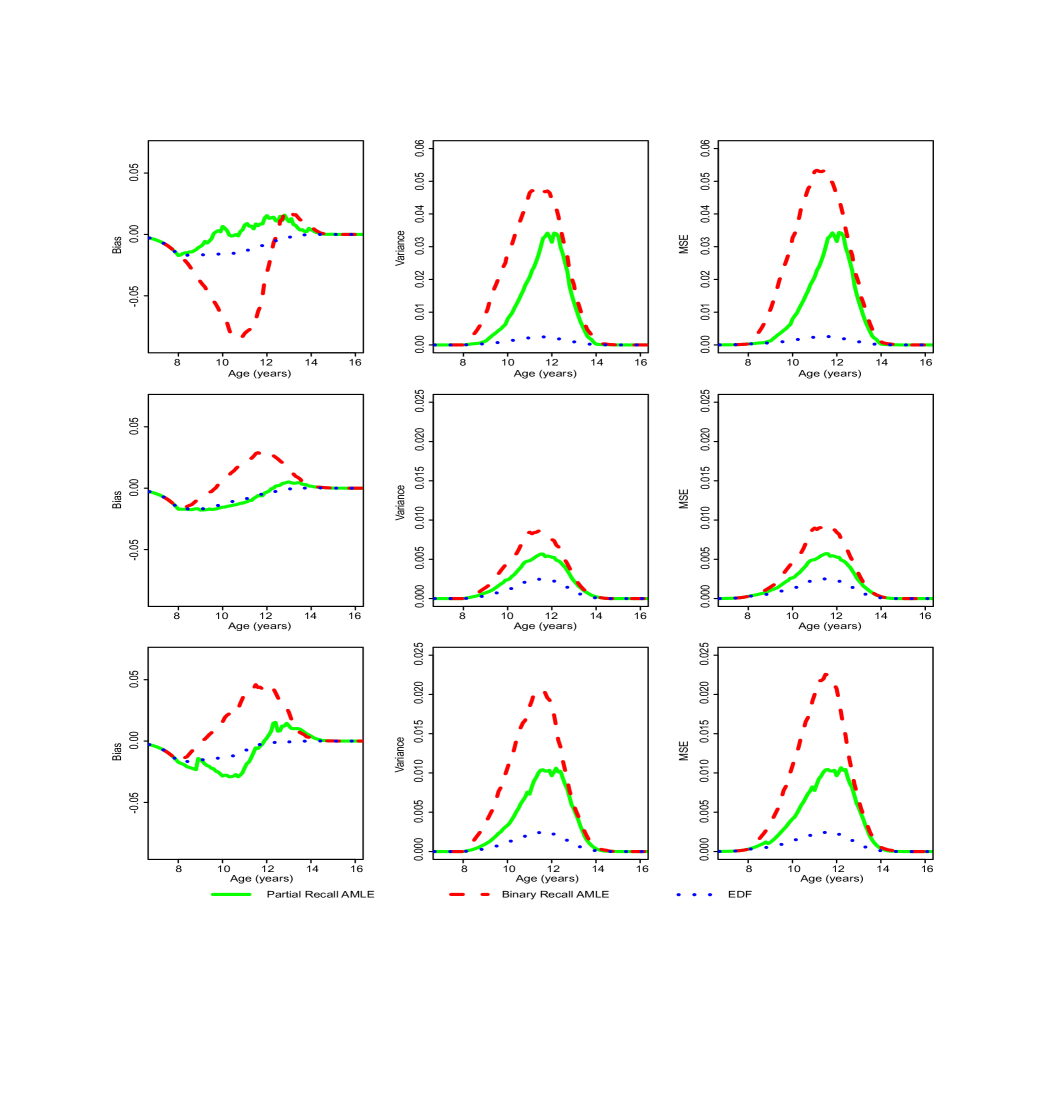
Figure 2 shows plots of the bias, the variance and the mean square error (MSE) of the three estimators for different ages, when $n=100$ and parameters of the recall functions (4.1) are chosen as in Cases (a), (b) and (c). The Partial Recall AMLE is found to have smaller bias, variance and MSE than the Binary Recall AMLE, although its performance is expectedly poorer than that of the EDF.

Plots similar to Figure 2 for $n=300$ and 1000 are given in the supplementary material. At those sample sizes, the performance parameters of partial AMLE are found to be closer to those of EDF than those of binary AMLE.

Figure 2: Comparison of bias, variance and MSE of the estimator for $n=100$ in cases (a) (top panel), (b) (middle panel) and (c) (bottom panel)

6 Adequacy of the Model

One can use the chi-square goodness of fit test to check how well the assumed parametric model actually fits the data. For this purpose, the data may be transformed to the vector $Y=(S,V,\varepsilon,\delta,m,d)$, and the support of the distribution of this vector may be appropriately partitioned, depending on the availability of data. An example is given in the next section.

Modeling of the recall probability functions is a critical issue. One has to choose suitable functional forms, and also strike a balance between a flexible model and a parsimonious one with fewer parameters. We provide below an exploratory technique for selecting the functional forms.

As we have seen in Section 4, use of the piecewise constant form (4.1) of the recall probabilities reduces the likelihood (5) to the likelihood (17). If the distribution of $T$ is known, one can obtain the MLE of the parameters $b_{l1},b_{l2},\ldots,b_{lk},\ l=0,1,2,3$. The conditional MLE of the piecewise constant functions $\pi^{(1)},\pi^{(2)},\pi^{(3)}$ and $\pi^{(0)}$, for any given $F_{\theta}$ can be obtained iteratively. By using a candidate parametric form $\pi_{\eta}^{(1)},\pi_{\eta}^{(2)},\pi_{\eta}^{(3)}$ and $\pi_{\eta}^{(0)}$, one can first estimate the MLEs $\hat{\theta}$ and $\hat{\eta}$ and then compare the plots of $\hat{\pi}_{\eta}^{(1)},\hat{\pi}_{\eta}^{(2)},\hat{\pi}_{\eta}^{(3)}$ and $\hat{\pi}_{\eta}^{(0)}$ with the plots of the conditional MLE of the piecewise constant versions of $\pi^{(1)},\pi^{(2)},\pi^{(3)}$ and $\pi^{(0)}$, with $F_{\theta}$ held fixed at $F_{\hat{\theta}}$. An example of this graphical check is given in the next section.

In addition, comparative plots of $F_{\hat{\theta}}$ computed for an assumed form of the recall probability functions and the piecewise constant forms mentioned in Section 4.1, can also serve as a graphical check of the adequacy of that assumed form. An example of this graphical check for the data set of next section is given in the supplementary material.

7 Data Analysis

For the data set described in Section 1, the landmark event is the onset of menarche in young and adolescent females. In a parametric analysis, we used the Weibull model for menarcheal age and the multinomial logistic model for the recall probabilities $\pi_{\eta}^{(0)},\pi_{\eta}^{(1)},\pi_{\eta}^{(2)}$ and $\pi_{\eta}^{(3)}$, as in Section 5.1. We used the three different methods mentioned in Section 5.1 for estimating the parameters $\theta_{1}$ and $\theta_{2}$ as well as the median of the age at menarche. Table 2 gives a summary of the findings. The Partial Recall MLEs have smaller standard errors than those of the other two estimators.

Table 2: Different estimates of parameters for the menarcheal data

Estimator	$\theta_{1}$ (Stdev)	$\theta_{2}$ (Stdev)	Median (Stdev)
Current Status MLE	19.05 (5.31)	11.65 (0.20)	11.42 (0.043)
Binary Recall MLE	10.32 (0.91)	12.27 (0.15)	11.84 (0.025)
Partial Recall MLE	9.432 (0.61)	12.25 (0.12)	11.78 (0.010)

Figure 3: Survival functions for the menarcheal data based on five methods

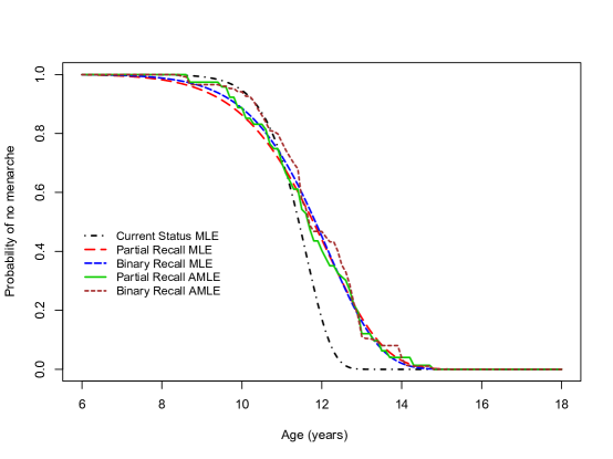
Figure 3 shows the survival functions estimated from the three parametric methods, the Partial Recall AMLE presented in Section 4.3 (with knot points of the recall probability functions chosen as in the first paragraph of Section 5.2) and Binary Recall AMLE (with the same knot points). The parametric MLEs are not very far from the non-parametric AMLEs. Though there appears to be little difference between the Partial Recall and Binary Recall MLEs, their standard errors are different (check Figure 3 of supplementary material).

In order to formally check how well the assumed parametric model fits the data, we use the chi-square goodness of fit test, by discretizing the range of the hexatuple $(S,V,\varepsilon,\delta,m,d)$. The range of $S$ is split into the intervals $[7,14]$ and $(14,21]$, the range of $d$ is split into the intervals $[0,1/24]$ and $(1/24,1/12]$, while the range of $V$ is split into the sets $[0,11.84]$ and $(11.84,21]$ ($11.84$ being the median of the observed non-zero values of $V$). The ranges of $\varepsilon$ and $\delta$ have four points ($0$, $1$, $2$ and $3$) and two points ($0$ and $1$), respectively, none of which are clubbed. The range of $m$ is the interval $[0,11]$, which is not split. When $\delta=0$, the value of $\varepsilon$ is irrelevant and $V=0$, i.e., there are four bins for the two groups of values of $S$ and two groups of $d$. When $\delta=1$ and $\varepsilon=3$, $V$ can only be zero and again there are only four bins. When $\delta=1$ and $\varepsilon=0,1$ or 2, in each case there are eight bins arising from two groups of values of $S$ and two groups of non-zero values of $V$ and $d$. Thus, we have a total of 32 bins.

In order to avoid small expected frequency in some cells we merge some bins where expected frequency is less than $5$. After this pruning, we have a reduced total of 21 bins. There are 8 parameters to estimate. Thus, the null distribution should be $\chi^{2}$ with 12 degrees of freedom. The p–value of the test statistic for the given data happens to be 0.169. Therefore, violation of the chosen model is not indicated.

Figure 4: Comparison of estimated logistic recall probabilities with estimated piecewise constant recall probabilities with (a) 4 pieces, (b) 8 pieces

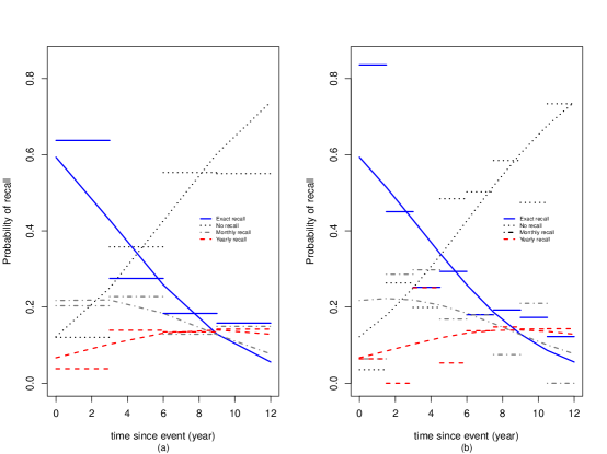
We now check the adequacy of the functional form of the $\pi_{\eta}^{(l)}$s by comparing the $\pi_{\hat{\eta}}^{(k)}$s with the conditional MLE of the corresponding piecewise constant function in (4.1), as indicated in the last section. For the given data, the largest value of $S_{i}-T_{i}$ in a perfectly recalled case happens to be 10.88 years. Therefore, we consider recall functions over the interval 0 to 12 years. With $F$ chosen as Weibull and $\theta_{1}$ and $\theta_{2}$ fixed at the values reported in the last row of Table 2, we obtained the conditional MLE of the values of $\pi_{\eta}^{(0)}$, $\pi_{\eta}^{(1)}$, $\pi_{\eta}^{(2)},\pi_{\eta}^{(3)}$ in different segments of equal length. Figure 4(a) shows the plots of the estimated recall probabilities under the logistic and the piecewise constant models, with number of segments $L=4$. The estimated functions are found to be close to each other for $l=0,1,2,3$. Figure 4(b) shows the same plots for $L=8$. The finer partition seems unnecessary. As another check of the functional form of the recall probability, we estimated the survival functions of time-to-event from the proposed parametric method using the multiple logistic regression model presented in Section 5.1 and the piecewise constant recall probability model introduced in Section 4.1 (with knot points of the recall probability functions chosen as in the first paragraph of Section 5.2). Figure 4 of supplementary material shows the two estimates of the survival function, which happen to be very close to each other.

We have seen the cumulative proportions of decreasing degrees of recall for different age ranges in the case of the menarcheal data in Figure 1. As an additional check for the assumed model, we consider the model based estimates of these cumulative proportions for ages $s=11,14,17$ and 20 (i.e., at the middle of the respective age intervals). We used the Partial Recall MLE of parameters $\hat{\theta}$ and $\hat{\eta}$ to calculate $f_{\hat{\theta}}$ and $\pi_{\hat{\eta}}^{(j)}$ for $j=0,1,2,3$ and then computed the requisite probabilities through numerical integration. Figure 5 shows the cumulative proportions in different age groups (solid lines) along with the corresponding model based estimates (dashed lines). The estimated probabilities are quite close to the empirical proportions.

Figure 5: Cumulative proportions (solid lines) and model based estimated probabilities (dashed lines) of decreasing degrees of recall in menarcheal data

8 Concluding Remarks

The aim of this paper has been to offer a realistic model for time-to-event based on partial recall information through an informative censoring model, where the range of relevant dates may depend on calendar time (rather than time elapsed since the event). The simulations and the data analysis of the menarcheal data set show that there is much to be gained from partial recall information in the form of the event falling in a calendar month or a calendar year. Many other forms of partial recall information may be handled in a similar way. As the simulations reported in Section 5 show, a particular category of partial recall (eg. recall up to a calendar month or year) is justified if that category is not very rare in the data.

The recalled time-to-event can sometimes be erroneous. Grouping of the uncertainly recalled event date by the calendar month or year may reduce the error to some extent. If one adopts this solution, the method presented in this paper provides a viable method of analysis. Skinner and Humphreys (1999), while working with data without instances of non-recall, has modeled erroneously recalled time-to-event as $t^{\prime}_{i}=t_{i}k_{i}$, where $t_{i}$ is the correct time-to-event and $k_{i}$ is a multiplicative error of recall that is independent of $t_{i}$. Since $k_{i}$s are unobservable, they have used a mixed-effects regression model to account for erroneous recalls. One may investigate whether a similar adjustment in the term $f_{\theta}(T_{i})$ of the likelihood (5), improves the analysis.

The Cox regression model has been adapted to the retrospective recall model for binary recall data (Mirzaei and Sengupta, 2015), and an adaptation to partial recall would be interesting. The multiple logistic regression model provides a framework for incorporating covariate effect on the recall probabilities also. These problems will be taken up in future.

9 Software

Software in the form of R code, together with the data set and complete documentation is available at GitHub (https://github.com/rahulfrodo/PartialRecall).

10 Supplementary Material

Supplementary material is available online at http://biostatistics.oxfordjournals.org.

11 Acknowledgements

This research is partially sponsored by the project “Physical growth, body composition and nutritional status of the Bengal school aged children, adolscents, and young adults of Calcutta, India: Effects of socioeconomic factors on secular trends”, funded by the Neys Van Hoogstraten Foundation of the Netherlands. The authors thank Professor Parasmani Dasgupta of the Biological Anthropology Unit of ISI, for making the data available for this research. The authors thank an anonymous referee and an associate editor for suggesting useful changes that improved the content and the presentation of the paper.

References

- Ash (2000) Ash, R. B. (2000). Probability and Measure Theory.. Burlington, MA: Harcourt/Academic Press.
- Dasgupta (2015) Dasgupta, P. (2015). Physical growth, body composition and nutritional status of bengali school aged children, adolescents and young adults of calcutta, india: Effects of socioeconomic factors on secular trends. (in collaboration with m. nubé, d. sengupta and m. de onis).
- Efron (1967) Efron, B. (1967). The two sample problem with censored data. Proceedings of the 5th Berkeley Symposium on Mathematical Statistics and Probability, 831–853.
- Gillespie and others (2006) Gillespie, B., dÁrcy, H., Schwartz, K., Bobo, J. K. and Foxma, B. (2006). Recall of age of weaning and other breastfeeding variables. International Breastfeeding Journal 1, 4.
- Harel and others (1994) Harel, Y., Overpeck, M. D., Jones, D. H., Scheidt, P. C., Bijur, P. E., Trumble, A. C. and Anderson, J. (1994). The effects of recall on estimating annual nonfatal injury rates for children and adolescents. American Journal of Public Health 84(4), 599–605.
- Joffe and others (1995) Joffe, M., Villard, .L, Li, Z., Plowman, R. and Vessey, M. (1995). A time to pregnancy questionnaire designed for long term recall: validity in oxford, england. Journal of Emidemiology and Community Health 49, 314–319.
- Koo and Rohana (1997) Koo, M. M. and Rohana, T. E. (1997). Accuracy of short-term recall of age at menarche. Annals of Human Biology 24, 61–64.
- Lee and Wang (2003) Lee, E. T. and Wang, J. W. (2003). Statistical Methods for Survival Data Analysis.. New York: John Wiley.
- Mathiowetza and Ouncanb (1988) Mathiowetza, N. A. and Ouncanb, G. J. (1988). Out of work, out of mind: Response errors in retrospective reports of unemployment. Journal of Business & Economic Statistics 6(2), 221–229.
- Mirzaei and Sengupta (2015) Mirzaei, S. S. and Sengupta, D. (2015). Regression under Cox’s model for recall-based time-to-event data in observational studies. Computational Statistics & Data Analysis, to be published, DOI:10.1016/j.csda.2015.07.005.
- Mirzaei and Sengupta (2016) Mirzaei, S. S. and Sengupta, D. (2016). Nonparametric estimation of time-to-event distribution based on recall data in observational studies. Lifetime Data Analysis 22, 473–503.
- Mirzaei and others (2015) Mirzaei, S. S., Sengupta, D. and Das, R. (2015). Parametric estimation of menarcheal age distribution based on recall data. Scandinavian Journal of Statistics 42, 290–305.
- Nocedal and Wright (2006) Nocedal, J. and Wright, S. J. (2006). Numerical Optimization. New York: Springer.
- Skinner and Humphreys (1999) Skinner, C. J. and Humphreys, K. (1999). Weibull regression for lifetimes measured with error. Lifetime Data Analysis 5, 23–37.
- Turnbull (1976) Turnbull, B. W. (1976). The empirical distribution function with arbitrarily grouped, censored and truncated data. Journal of the Royal Statistical Society, Series B 38, 290–295.