Common pulse retrieval algorithm: a fast and universal method to retrieve ultrashort pulses

Abstract

We present a common pulse retrieval algorithm (COPRA) that can be used for a broad category of ultrashort laser pulse measurement schemes including frequency-resolved optical gating (FROG), interferometric FROG, dispersion scan, time domain ptychography, and pulse shaper assisted techniques such as multiphoton intrapulse interference phase scan (MIIPS). We demonstrate its properties in comprehensive numerical tests and show that it is fast, reliable and accurate in the presence of Gaussian noise. For FROG it outperforms retrieval algorithms based on generalized projections and ptychography. Furthermore, we discuss the pulse retrieval problem as a nonlinear least-squares problem and demonstrate the importance of obtaining a least-squares solution for noisy data. These results improve and extend the possibilities of numerical pulse retrieval. COPRA is faster and provides more accurate results in comparison to existing retrieval algorithms. Furthermore, it enables full pulse retrieval from measurements for which no retrieval algorithm was known before, e.g., MIIPS measurements.

1 Introduction

Since the advent of ultrashort laser pulses there has been ongoing research on techniques to determine their temporal structure. Nowadays, there is quite literally a "zoo" of techniques available for that purpose [1].

The direct measurement of the temporal intensity of laser pulses using electrical detectors is limited to the picosecond range due to their relatively slow response time. Autocorrelation measurements [2, 3] were introduced to overcome this limitation and are still the most widely used pulse characterization methods. However, it is not possible to retrieve the full pulse information from a single autocorrelation measurement, as it is ambiguous with respect to the pulse amplitude and phase [4].

A prominent method, which enables the reconstruction of both the pulse amplitude and phase, is called frequency-resolved optical gating (FROG) [5, 6]. It extends the non-collinear intensity autocorrelation by measuring the spectrum of its nonlinear signal for every delay. The most common variant of FROG utilizes non-collinear second harmonic generation (SHG). The resulting two-dimensional measurement, a set of frequency-doubled spectra, is called the SHG-FROG trace. It is presumed to uniquely define both pulse amplitude and phase except for certain, so-called trivial, ambiguities [7, 8].

Several variants of FROG exist that use other nonlinear processes such as third-harmonic generation (THG), self-diffraction (SD) and polarization gating (PG) [6]. An interferometric variant of SHG-FROG that is based on the collinear autocorrelation is called interferometric FROG (iFROG) [9]. Recently it has been demonstrated by using THG as the nonlinear process [10, 11].

Reconstructing a pulse from a FROG trace measurement requires an iterative algorithm. One successful approach was inspired by projection on convex sets [12] and is called the generalized projections algorithm (GPA) [13]. An improved version that exploits the specific algebraic structure of a FROG trace for faster retrieval is called the principal components generalized projections algorithm (PCGPA) [14].

A more recent pulse measurement technique is dispersion scan (d-scan) which has become a valuable tool for few-cycle pulse measurement [15, 16]. In this method the pulses are chirped by inserting an adjustable dispersive element, e.g., a pair of glass wedges, into the beam path and their SHG spectrum is measured as a function of the induced chirp to form the d-scan trace. The pulse can then be retrieved from the trace by using a multi-dimensional optimization algorithm. The technique was also demonstrated using THG and inline SD as the nonlinear process [17, 18]. Recently a fast, iterative algorithm based on generalized projections was proposed to enable pulse retrieval from SHG and THG d-scan traces [19].

A third class of pulse measurement methods can be implemented using a pulse shaper. With this a set of spectral phase masks is applied to the pulses. Then the SHG spectrum for every phase mask is measured to obtain a two-dimensional measurement trace. The most prominent technique in this class is called multiphoton intrapulse interference phase scan (MIIPS) [20, 21], where sinusoidal phase patterns with varying shifts are applied. So far, only iterative spectral phase compensation has been demonstrated by using an algorithm that extracts an approximation to the second derivative of the spectral phase from the measurement. Other techniques represent adaptations of existing measurement schemes to the use with a pulse shaper [22, 23, 24, 25].

Time-domain ptychography (TDP) is a recently developed pulse measurement technique [26, 27, 28]. It is inspired by a coherent diffractive imaging technique of the same name [29]. It uses a correlation setup similar to FROG where the pulse in one arm is spectrally filtered. The pulse retrieval algorithms used for TDP are an adaption of the image retrieval algorithms in spatial ptychography [30, 31]. They have also been successfully applied to cross-correlation FROG (XFROG) [32] and SHG-FROG [33, 34].

Typically, each family of these pulse measurement methods comprises both a specific experimental setup and a taylored retrieval algorithm, which makes them difficult to compare. They are, however, structurally similar. For that reason, our paper starts in Sec. 2 by developing a common formalism for what we call parametrized nonlinear process spectra (PNPS) measurements. It allows to describe most self-referenced techniques for ultrashort pulse measurement using the same formalism. It forms the basis of our work and is used to develop all arguments in the following sections.

The main idea of our paper is presented in Sec. 3. We discuss PNPS pulse retrieval as a nonlinear least-squares problem. We propose this as the natural way to view the pulse retrieval problem and stress that the least-squares solution is ideal under the assumption of Gaussian noise.

The main result of our paper is the common pulse retrieval algorithm (COPRA) described in Sec. 4. It can be applied universally to all PNPS measurements. It is in general faster than general least-squares solvers and more accurate than other specialized pulse retrieval algorithms. It significantly extends the possibilities of numerical pulse retrieval because for some PNPS measurements no fast retrieval algorithm was known before (e.g., SD-dscan) and for some no phase and amplitude retrieval algorithm existed at all (e.g., MIIPS).

In Secs. 5 and 6 we describe the comprehensive numerical tests that were performed to verify and demonstrate the properties of COPRA. They included testing the retrieval for various PNPS measurements, test pulses and levels of noise. For SHG-FROG we compare it to PCGPA and ptychographic retrieval. We can show that those algorithms do not converge on a least-squares solution and, consequently, are much less accurate in the presence of Gaussian measurement noise. We also demonstrate that COPRA is able to retrieve pulses from incomplete traces. Furthermore, we evaluate the applicability of general minimization algorithms on the pulse retrieval problem. We find that gradient-based algorithms such as Levenberg-Marquadt are generally superior to gradient-free methods.

In Sec. 7 we summarize the results and give an outlook on future work. In the supplementary material we also give more details and technical aspects that facilitate the application and reimplementation of COPRA.

2 Concepts

In this section we introduce a unified description of most self-referenced pulse measurement methods. It is based on the observation that the measured quantity is the same for all methods mentioned in the introduction: a set of pulse spectra after a nonlinear process. Specifically, the nonlinear process is tunable by some parameter that forms the second measurement dimension. For example, for SHG-FROG the parameter is the pulse delay and the nonlinear process a non-collinear SHG. For SHG-d-scan the parameter is the insertion distance of a glass wedge and the nonlinear process is a collinear SHG.

We call these measurements parametrized nonlinear process spectra (PNPS) measurements. Other pulse measurement techniques exist that cannot be described in this way. Most prominently this pertains to spectral phase-interferometry for direct electric field reconstruction (SPIDER) [35] and other methods based on spectral interferometry. They do not require a retrieval algorithm and are not subject of this paper.

2.1 Continuous PNPS formalism

We work with the complex-valued pulse envelope $E(t)$ and its spectral counterpart $\tilde{E}(\omega)$, where $\omega=\varOmega-\varOmega_{0}$ is the centered frequency and $\varOmega_{0}$ the central frequency. Both are related by the Fourier transform and its inverse using the following convention

$$\tilde{E}(\omega) =\mathcal{F}\mathopen{}\left[E\right](\omega)=\frac{1}{2\pi}\int_{-\infty}^{\infty}E(t)\>\mathrm{e}^{\mathrm{i}\omega t}\mathrm{d}t,$$ (1)

$$E(t) =\mathcal{F}^{\raisebox{0.60275pt}{$\scriptscriptstyle-1$}}\mathopen{}\left[\tilde{E}\right](t)=\int_{-\infty}^{\infty}\tilde{E}(\omega)\>\mathrm{e}^{-\mathrm{i}t\omega}\mathrm{d}\omega.$$ (2)

All PNPS traces $T$ can be modeled by the following equation

$$T(\delta,\omega;\tilde{E})=\left|\mathcal{F}\mathopen{}\left\{\mathcal{S}\mathopen{}_{\delta}\left[\tilde{E}\right](t)\right\}(\omega)\right|^{2}.$$ (3)

$T$ depends on the pulse $\tilde{E}$ and is evaluated at the frequency $\omega$ and the parameter $\delta$. $\mathcal{S}\mathopen{}_{\delta}$ is the signal operator that describes a parametrized nonlinear process in the time domain. $\delta$ is a method-specific parameter that tunes the nonlinear process.

Depending on the structure of the signal operator we distinguish between non-collinear methods (e.g., FROG or TDP) and collinear methods (e.g., d-scan or iFROG). Examples of the signal operator in the former case can be found in Tab. 1. In the latter case we can decompose the signal operator in the following way

$$\mathcal{S}\mathopen{}_{\delta}[\tilde{E}](t)=\mathcal{N}\mathopen{}\left\{\mathcal{F}^{\raisebox{0.60275pt}{$\scriptscriptstyle-1$}}\mathopen{}\left[\tilde{H}_{\delta}\>\tilde{E}\right]\right\}(t).$$ (4)

$\tilde{H}_{\delta}(\omega)$ is the parametrization filter and describes a parametrized linear operation in the frequency domain. Examples are listed in Tab. 2. $\mathcal{N}\mathopen{}$ is the nonlinear process operator and describes the subsequent conversion of a pulse by a collinear nonlinear process. Expressions for the processes commonly used in pulse measurement can be found in Tab. 3.

PNPS traces do not uniquely define a pulse. For example, they are all ambiguous to the constant and linear phase of $\tilde{E}(\omega)$. Some methods (e.g., SHG-FROG and SHG-iFROG) leave the direction of time undetermined. Additionally, the relative phase of pulse components well-separated in frequency can be shown to be ambiguous, similar to how it was done for FROG [36]. Answering the underlying question if a PNPS trace is essentially unique, i.e., if it defines pulse amplitude and phase up to a set of known, so-called trivial ambiguities, is out of scope for this work. Even for the well-studied FROG method it is still a topic of ongoing research [7, 8, 37]. We will take a pragmatic approach and test for non-trivial ambiguities by numerically retrieving pulses from a large number of synthetic measurements.

Table 1: Signal operator for selected non-collinear schemes.

Method	$\mathcal{S}\mathopen{}_{\tau}[\tilde{E}]$
SHG-FROG	$\mathcal{F}\mathopen{}^{-1}\left[\mathrm{e}^{\mathrm{i}\tau\omega}\tilde{E}\right]\>\mathcal{F}\mathopen{}^{-1}\left[\tilde{E}\right]$
PG-FROG	$\left|\mathcal{F}\mathopen{}^{-1}\left[\mathrm{e}^{\mathrm{i}\tau\omega}\tilde{E}\right]\right|^{2}\>\mathcal{F}\mathopen{}^{-1}\left[\tilde{E}\right]$
TDPa	$\mathcal{F}\mathopen{}^{-1}\left[\mathrm{e}^{\mathrm{i}\tau\omega}\tilde{B}(\omega)\tilde{E}\right]\>\mathcal{F}\mathopen{}^{-1}\left[\tilde{E}\right]$

The pulse delay $\tau$ is the parameter $\delta$ in these methods. More examples can be found in the supplementary material. ^a$\tilde{B}(\omega)$ describes the transmission of a bandpass filter used in the scheme.

Table 2: Parametrization filter for selected collinear schemes.

Scheme	Parameter $\delta$	$\tilde{H}_{\delta}(\omega)$
d-scana	glass insertion $z$	$\exp[\mathrm{i}k(\omega+\varOmega_{0})z]$
MIIPSb	pattern shift $\delta$	$\exp[\mathrm{i}\alpha\cos(\gamma\omega-\delta)]$
iFROG	delay $\tau$	$1/2+\exp[\mathrm{i}\tau(\omega+\varOmega_{0})]/2$

More examples can be found in the supplementary material. ^a$k(\varOmega)$ depends on the material of the wedges and is usually defined by Sellmeier equations. ^b$\alpha$ and $\gamma$ are free parameters of the method and have to be adapted to the measured pulses.

Table 3: Nonlinear process operators for collinear schemes.

Process	SHG	THG	SD
$\mathcal{N}\mathopen{}[E]$	$E^{2}$	$E^{3}$	$\left|E\right|^{2}E$

2.2 Discrete PNPS formalism

To perform pulse retrieval we have to a introduce a discrete version of the PNPS formalism. We define equidistant simulation grids with $N$ points in time and frequency

$$t_{n} \equiv t_{0}+n\>\Delta t,\quad n=0,\ldots,N-1$$ (5)

$$\omega_{n} \equiv\omega_{0}+n\>\Delta\omega.$$ (6)

We set $E_{n}\equiv E(t_{n})$ and $\tilde{E}_{n}\equiv\tilde{E}(\omega_{n})$. We use $\mathbf{E}\equiv(E_{0},\ldots,E_{N-1})$ and $\mathbf{\tilde{E}}\equiv(\tilde{E}_{0},\ldots,\tilde{E}_{N-1})$ to denote the whole pulse. The Fourier transform is approximated by discrete evaluation of the integral and is denoted by

$$\tilde{E}_{n}=\mathrm{FT}_{{k}\shortrightarrow{n}\mathopen{}}(E_{k})\quad\text{and}\quad E_{k}=\mathrm{FT}_{{n}\shortrightarrow{k}\mathopen{}}^{\raisebox{0.60275pt}{$\scriptscriptstyle-1$}}(\tilde{E}_{n}).$$ (7)

We have $M$ spectra for the parameters $\delta_{0},\ldots,\delta_{M-1}$. There is no restriction on the number, spacing or position of the tuning parameters $\delta_{m}$, e.g., as it is required by PCGPA for FROG. The discrete PNPS signal $S_{mk}$ is defined by a discrete evaluation of the signal operator at $\delta_{m}$ and $t_{k}$:

$$S_{mk}\equiv S_{mk}(\mathbf{\tilde{E}})\approx\mathcal{S}\mathopen{}_{\delta_{m}}[\tilde{E}](t_{k}).\quad\begin{split}m&=0,\ldots,M-1\\ k&=0,\ldots,N-1\end{split}$$ (8)

Its counterpart in the frequency domain is denoted by

$$\tilde{S}_{mn}\equiv\tilde{S}_{mn}(\mathbf{\tilde{E}})=\mathrm{FT}_{{k}\shortrightarrow{n}\mathopen{}}(S_{mk}),\quad\begin{split}m&=0,\ldots,M-1\\ n&=0,\ldots,N-1\end{split}$$ (9)

Finally, we can calculate the discrete PNPS trace $T_{mn}$ by

$$T_{mn}\equiv T_{mn}(\mathbf{\tilde{E}})=|\tilde{S}_{mn}(\mathbf{\tilde{E}})|^{2}\approx T(\delta_{m},\omega_{n};\tilde{E}).$$ (10)

The measurement from which the pulse is reconstructed, the measured PNPS trace, is denoted by $T^{\mathrm{meas}}_{mn}$. More details on how the calculations are performed can be found in the supplementary material (Sec. S2).

3 Pulse retrieval problem

Figure 1: a) A diagram of the discrete PNPS formalism. b) First stage of COPRA: local iteration c) Second stage of COPRA: global iteration.

The discrete pulse retrieval problem is to find the pulse $\mathbf{\tilde{E}}$ that gives rise to a PNPS trace $T_{mn}$ that matches the measurement $T^{\mathrm{meas}}_{mn}$. As $T^{\mathrm{meas}}_{mn}$ is subject to measurement errors the retrieval will never be exact and we need to choose a metric to select the best solution.

In this work we view pulse retrieval as a nonlinear least-squares problem. It is a nonlinear inverse problem and solving such problems in the least-squares sense is very well-established and understood [38]. Under the assumption of Gaussian measurement errors the least-squares solution represents an optimal choice, namely the maximum-likelihood estimate [39] and a Gaussian distribution is usually a good model for noise in spectrometric measurements [40].

To explain why we put so much emphasis on finding a least-squares solution we have to anticipate a key result from Sec. 6.6.2. We found that retrieval algorithms based on generalized projections or ptychography do not converge onto a solution in the least-squares sense. These methods use the sum of squared residuals, e.g., the FROG error $G$, to assess and select a solution. However, they minimize it only approximately. In consequence, they under-perform in the presence of additive Gaussian noise. This fact has been noticed several times in the literature [25, 19, 11, 41], but the relation to the missing least-squares property was not reported so far.

With this in mind we state the pulse retrieval problem as fitting the $2N$ independent variables in $\mathbf{\tilde{E}}$ (real and imaginary parts) to $MN$ dependent variables in $T^{\mathrm{meas}}_{mn}$ by minimizing the sum of squared residuals $r$

$$r\equiv r(\mathbf{\tilde{E}})=\sum_{m,n}\left[T^{\mathrm{meas}}_{mn}-\mu T_{mn}(\mathbf{\tilde{E}})\right]^{2}.$$ (11)

Throughout the paper we use the trace error $R$ defined by

$$R\equiv R(\mathbf{\tilde{E}})=r^{1/2}/\bigl{[}MN\>(\operatorname*{max}_{m,n}T^{\mathrm{meas}}_{mn})^{2}\bigr{]}^{1/2}$$ (12)

to assess the convergence. $R$ is the normalized root-mean-square error (NRMSE) between $T^{\mathrm{meas}}_{mn}$ and $\mu T_{mn}$. The normalization facilitates the comparison of $R$ between different measurements and PNPS schemes. In the FROG literature $\max T^{\mathrm{meas}}=1$ is usually assumed implicitly and, thus, $R$ is then equivalent to the FROG error $G$.

The scaling factor $\mu$ in (11) accounts for different scales of the measured and computed traces. Its value can be obtained for every $\mathbf{\tilde{E}}$ from an analytical solution by

$$\mu=\sum_{m,n}\left[T^{\mathrm{meas}}_{mn}\>T_{mn}(\mathbf{\tilde{E}})\right]/\sum_{m,n}T_{mn}(\mathbf{\tilde{E}})^{2}.$$ (13)

A general solution strategy for the pulse retrieval problem is to minimize $r$ by employing a nonlinear minimization algorithm as demonstrated in Sec. 6.6.1. However, in general such an approach will be less efficient than a specialized algorithm like the one we present in the next section.

4 Common pulse retrieval algorithm

In the following we present a fast iterative pulse retrieval algorithm that is able to solve the PNPS pulse retrieval problem in the least-squares sense. We call it the common pulse retrieval algorithm (COPRA).

Once the algorithm is implemented it can easily be applied to a multitude of present and future PNPS methods. The only parts that actually depend on the measurement scheme are the calculation of $T_{mn}$ and of one gradient (see (16)). For collinear schemes only the expression for $\tilde{H}(\delta_{m},\omega_{n})$ has to be replaced.

Convergence on the global minimum is not guaranteed with COPRA. In principle, it has to be restarted repeatedly from different initial values. However, it was designed to achieve high retrieval probabilities even for totally random initial guesses. With an informed initial guess usually a single run of COPRA is sufficient (see Sec. 6.6.2).

In a setup step the trace error $R$ and the scaling factor $\mu$ from (13) are calculated for the initial guess. Furthermore, the maximum local gradient norm $g^{0}_{M-1}$ (see next section) has to be calculated here before the algorithm starts with the first of two stages.

4.1 Stage I: local iteration

In the first stage all steps are performed subsequently on one spectrum at a time, i.e., $m$ is constant below. Hence, we call this stage local iteration. The spectra are processed in random order, but for notations sake we assume that we start with $m=0$ and end with $M-1$. The corresponding one-dimensional measurement signal $S_{mk}$ and its spectrum $\tilde{S}_{mk}$ are calculated by Eqs. (8-9). Next a projection on the measured intensity is performed. For that the amplitude of $\tilde{S}_{mk}$ is replaced by the measured one from $T^{\mathrm{meas}}_{mn}$, followed by an inverse Fourier transform to obtain a new measurement signal $S_{mk}^{\prime}$:

$$S_{mk}^{\prime}=\mu\>\mathrm{FT}_{{n}\shortrightarrow{k}\mathopen{}}^{\raisebox{0.60275pt}{$\scriptscriptstyle-1$}}\left(\tilde{S}_{mn}/|\tilde{S}_{mn}|\sqrt{T^{\mathrm{meas}}_{mn}}\right).$$ (14)

Note the use of the scaling factor $\mu$ here. We define the distance $Z_{m}$ between $S_{mk}^{\prime}$ and $S_{mk}$ as

$$Z_{m}=\sum_{k}\left|S_{mk}^{\prime}-S_{mk}(\mathbf{\tilde{E}})\right|^{2},$$ (15)

and try to minimize it in terms of the current solution $\mathbf{\tilde{E}}$. To that end, in iteration $j$ a single gradient descent step is performed for every spectrum $m$

$$\tilde{E}_{n}^{\prime}=\tilde{E}_{n}-\gamma_{m}^{j}\>\nabla_{n}Z_{m}.$$ (16)

The expressions for the gradient $\nabla_{n}Z$ for all PNPS methods discussed here are given in the supplementary material (Sec. S3). They can be evaluated using one or two additional fast Fourier transforms (FFT) depending on the scheme.

The algorithm proceeds to the next spectrum using the updated solution $\mathbf{\tilde{E}}^{\prime}$. If all spectra are processed one local iteration of the algorithm is finished. Additionally, after every iteration $R$ is calculated from $S_{mk}$ and $\mu$ is updated. The local iteration is stopped when no improvement of $R$ was achieved for ten iterations.

The step size $\gamma$ is crucial to the convergence of the local iteration. For traces without or with very little noise we found the following to work very well

$$\gamma=Z_{m}/\sum_{n}|\nabla_{n}Z_{m}|^{2}.$$ (17)

In the presence of noise, however, this choice leads to poor convergence. We found that reliable convergence for all noise levels can be achieved by exchanging the denominator. For that we keep track of the maximum gradient norm in every iteration $j$

$$g^{j}_{m}=\mathrm{max}\bigr{(}g^{j}_{m-1},\sum_{n}|\nabla_{n}Z_{m}|^{2}\bigl{)}\quad\text{with}\quad g^{j}_{-1}=0.$$ (18)

The step size in iteration $j$ is then defined by

$$\gamma_{m}^{j}=Z_{m}/\mathrm{max}(g^{j}_{m},g^{j-1}_{M-1}),$$ (19)

where $g^{j}_{m}$ is the running estimate for the maximum gradient norm in the current iteration and $g^{j-1}_{M-1}$ is the maximum gradient norm encountered during the last iteration. Before the first local iteration $g^{0}_{M-1}$ has to be determined separately in the setup step which counts as the first iteration $j=0$.

4.2 Stage II: global iteration

In the second stage all spectra are processed simultaneously in every step and $m$ runs from $0$ to $M-1$ in the expressions below. Hence, we call this stage global iteration. It is seeded by the best solution of the local iteration stage.

A global iteration starts by calculating $S_{mk}$, $\tilde{S}_{mn}$, and $T_{mn}$ for the current guess $\mathbf{\tilde{E}}$ by Eqs. (8-10). Then the trace error $R$ and the scale factor $\mu$ are computed by Eqs. (12-13). An updated signal $S_{mk}^{\prime}$ is obtained by minimizing $r$ from (11) in terms of $S_{mk}$. This is done by a single gradient descent step

$$S_{mk}^{\prime} =S_{mk}-\eta_{r}\>\nabla_{mk}r,$$ (20)

with

$$\eta_{r} =\alpha\bigl{(}r/\sum_{lj}|\nabla_{lj}r|^{2}\bigr{)},$$ (21)

where the gradient is given by

$$\nabla_{mk}r=-4\mu\frac{\Delta t}{2\pi\Delta\omega} \mathrm{FT}_{{n}\shortrightarrow{k}\mathopen{}}^{\raisebox{0.60275pt}{$\scriptscriptstyle-1$}}\left[\bigl{(}T^{\mathrm{meas}}_{mn}-\mu T_{mn}\bigr{)}\tilde{S}_{mn}\right].$$ (22)

We follow up by adapting $\mathbf{\tilde{E}}$ to this new estimate $S_{mk}^{\prime}$. This is done as in the local iteration, but all spectra are processed simultaneously. With

$$Z=\sum_{m}Z_{m}=\sum_{mk}\left|S_{mk}^{\prime}-S_{mk}(\mathbf{\tilde{E}})\right|^{2},$$ (23)

we have

$$\nabla_{n}Z=\sum_{m}\nabla_{n}Z_{m}.$$ (24)

We obtain the next estimate by a single gradient descent step

$$\tilde{E}_{n}^{\prime} =\tilde{E}_{n}-\eta_{z}\nabla_{n}Z,$$ (25)

with

$$\eta_{z} =\alpha\bigl{(}Z/\sum_{k}|\nabla_{k}Z|^{2}\bigr{)}.$$ (26)

The constant $\alpha$ controls the step size both in (21) and (26). We use $\alpha=0.25$ for all results shown in this work.

In this work we simply performed COPRA for a fixed number of total iterations. However, an arbitrary convergence criterion can be used instead to terminate the global iteration. After the algorithm has terminated, the solution with the lowest trace error $R$ is returned.

4.3 Design considerations

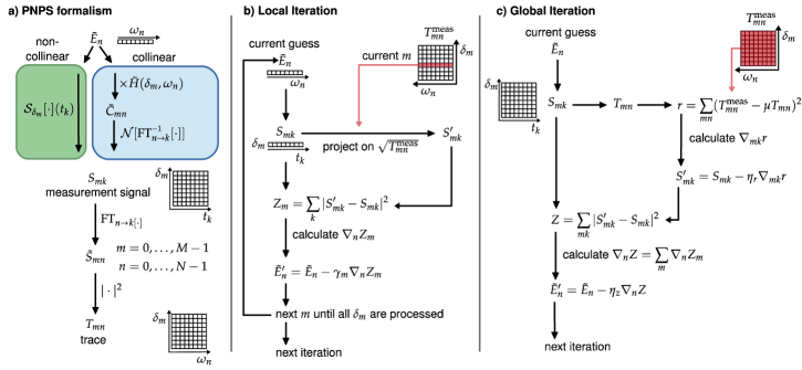
Fig. 1 summarizes the discrete PNPS formalism and shows diagrams of both stages of the algorithm. In the following we will discuss the overall design and implementation of the algorithm and how it relates to existing approaches.

The local iteration aims to provide an approximation of the solution in a rapid and reliable way. It is less likely to get stuck in a local minimum and the initial convergence is much faster than during the global iteration. For the noiseless case, i.e., on synthetic measurements, only this stage of COPRA is necessary. However, in the presence of noise it will fail to converge to a least-squares solution. This is why the global iteration has to be performed subsequently.

Our algorithm was inspired by GPA for FROG [13, 6]. For example, we minimize the same distance $Z$ in our algorithm. However, there are some key differences.

First of all, COPRA operates with the pulse spectrum $\mathbf{\tilde{E}}$ as the independent variable. Choosing the pulse field $\mathbf{E}$ would in general make the calculation of the PNPS trace and the required gradients more complicated.

Second, we found heuristically safe and divergence-free expressions for the step sizes. This avoids the overhead of determining them with a line search in every iteration.

Third, the local iteration processes one spectrum at a time. We found that this approach can increase the convergence speed and makes the algorithm less prone to stagnation.

Finally, the most important difference is that in the global iteration we replaced the projection on the measured intensity by a gradient descent step. This it what allows to obtain a least-squares solution which is not possible when using a projection on the measurement.

The local iteration is similar to ptychography-based algorithms for SHG-TDP [26] and SHG-FROG [33, 34], since the update step in ptychography is a gradient descent step [31]. However, the gradients used in ptychography are different, as the expression for SHG is seen as linear in two independent variables: the object and the probe pulse. Consequently, the gradient in ptychography is calculated with respect to one pulse only. This is only one of two terms used in our algorithm. This issue is discussed in detail in the supplementary material (Sec. S6).

5 Methods

For testing purposes we created an overall number of 100 random test pulses with a root-mean-square time-bandwidth product (TBP) of $2$. For comparison, the TBP of a Gaussian pulse with flat phase is $0.5$ in this definition. The pulses possess a complex amplitude and phase structure in both the time and frequency domain. The grid size was $N=256$. Retrieving such pulses represents a significant challenge for pulse retrieval algorithms and allows us to clearly assess the performance of our algorithm.

The specific central frequency ($\lambda_{0}=$800\text{\,}\mathrm{nm}$$) and the temporal grid spacing ($\Delta t=$5\text{\,}\mathrm{fs}$$) used in our simulations have no influence on the pulse retrieval. The results obtained here are applicable to other frequency and time scales, thus, we leave out the information on the frequency and time axes.

The algorithm was usually initialized by a Gaussian pulse with a duration of $50\text{\,}\mathrm{fs}$ (full width half maximum) and random spectral phase (uniformly distributed on $[-0.1\pi,0.1\pi]$). This matches realistic conditions where only rough knowledge about the pulse duration is available.

To test COPRA under stricter conditions we also used a completely random initial guess. Its spectral amplitude and phase were uniformly distributed on $[0,1]$ and $[0,2\pi]$ respectively. This makes no assumptions at all and allows for a fully unbiased estimation of the retrieval probability of the algorithm.

We quantified the retrieval accuracy by comparing the retrieved solution $\mathbf{\tilde{E}}$ to the test pulse $\mathbf{\tilde{E}}^{0}$ from which the synthetic measurement trace was generated. This was done by calculating the retrieval error $\varepsilon$, which is the NRMSE between both pulses. However, the ambiguity of the constant and linear spectral phase as well as the scaling have to be taken into account. This leads to the formal definition

$$\varepsilon(\mathbf{\tilde{E}}) \equiv\Bigl{[}\>\min_{\mu,\varphi_{0},\varphi_{1}}\sum_{n}|\tilde{E}_{n}^{0}-\mu\exp[\mathrm{i}(\varphi_{0}+\varphi_{1}\omega)]\tilde{E}_{n}|^{2}$$

$$\qquad/(N\>\max_{n}|\tilde{E}_{n}^{0}|^{2})\Bigr{]}^{1/2}.$$ (27)

Additionally, for some schemes the time-reversal ambiguity has to be considered, in which case $\varepsilon\equiv\min[\varepsilon(\mathbf{\tilde{E}}),\varepsilon(\mathbf{\tilde{E}}^{*})]$. The procedure of how $\varepsilon$ is calculated is described in the supplementary material (Sec. S4).

To investigate the influence of noise on the retrieval we added Gaussian noise to the synthetic measurement traces. The standard deviation $\sigma$ of the noise was chosen relative to the maximum intensity of the trace and is given in percent, e.g., $\sigma=1\%$. This noise model corresponds to a low intensity measurement with a CCD array spectrometer where signal-independent noise sources dominate [40]. Signal-dependent Gaussian noise requires to introduce a weighting in the pulse retrieval problem, which leads to small modifications in COPRA as is discussed in the supplementary material (Sec. S8).

In the noiseless case $R$ directly quantifies the convergence and is only limited by the accuracy of the trace computation. We assumed successful retrieval if a solution with $R<$110-4$$ was obtained. However, for noisy measurements $R$ will be on the order of the relative noise level, i.e., $\sigma=1\%$ leads to $R\approx 1\%$. To assess the convergence we compare it to the non-vanishing trace error of the test pulse $\mathbf{\tilde{E}}^{0}$ used to create the synthetic measurement

$$R_{0}\equiv R(\mathbf{\tilde{E}}^{0}).$$ (28)

This is an approximation of the expected trace error of the global least-squares solution. Specifically, we assume successful retrieval if $R<R_{0}+$110-4$$.

To assess the versatility of COPRA we tested it on a multitude of PNPS schemes, including common ones such as SHG-FROG, PG-FROG, SHG-TDP, SHG-d-scan, SHG-iFROG, as well as less common ones such as THG-d-scan, SD-d-scan and THG-iFROG. Furthermore, we included variants of MIIPS and iFROG, namely THG-MIIPS, SD-MIIPS and SD-iFROG, that to our knowledge have not yet been demonstrated experimentally. They serve to showcase COPRA’s universality.

For every scheme we selected an appropriate parameter set $\delta_{m}$. For FROG methods we chose to sample the delay $\tau$ like the pulse itself with $\tau_{m}=t_{m}$ and $M=N$. This is the common choice and the one required by PCGPA. For iFROG the same choice was used except when using SD as the nonlinear process. In this case we sampled $\tau$ at four times the frequency with $\Delta\tau=0.25\Delta t$ and $M=4N$. For the other schemes we sampled $\delta_{m}$ with $M=128$ points. For MIIPS the free parameters $\alpha$ and $\gamma$ had to be chosen appropriately. Details and the full list of parameters can be found in the supplementary material (Sec. S4).

For SHG-FROG we compare our algorithm to two other fast pulse retrieval algorithms: PCGPA and a recently proposed retrieval algorithm based on the ptychographic iterative engine (PIE) [33, 34]. We give details on this choice and their implementation in the supplementary material (Sec. S6).

6 Results

6.1 Nonlinear least-squares solvers

Figure 2: a) Synthetic SHG-FROG trace with $N=M=64$. b) Trace error obtained by four different minimization algorithms plotted over the number of full evaluations of the trace $T_{mn}$. Shown are the best out of ten runs for every algorithm.

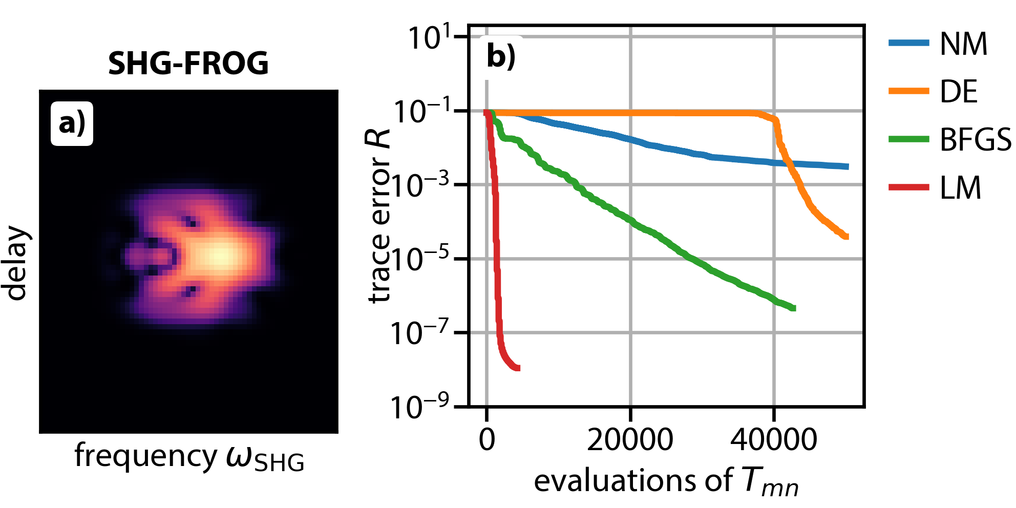
To demonstrate the applicability of general minimization algorithms to the pulse retrieval problem we created a simple SHG-FROG trace with $N=M=64$ belonging to a pulse with TBP 1 (see Fig. 2 a). Then we retrieved pulses by using four different minimization algorithms: Nelder-Mead (NM) and differential evolution (DE) are scalar, gradient-free minimization methods used to retrieve pulses from d-scan and iFROG measurements [15, 11, 41]. Broyden–Fletcher–Goldfarb–Shanno (BFGS) is a scalar, gradient-based algorithm, which was used to retrieve pulses from chirp scan and FROG measurements [25]. Furthermore, we tested the Levenberg-Marquadt (LM) algorithm, which is a specialized nonlinear least-squares solver. For both BFGS and LM numerical differentiation was used to approximate the derivatives. The additional trace evaluations required for that were factored into our comparison.

The convergence behavior in terms of trace evaluations for the best of the ten retrievals from random initial guesses is shown in Fig. 2 b). LM massively outperformed the other algorithms in terms of retrieval efficiency. For every run a solution ($R<$110-4$$) was found with an effort of less than $1500$ trace evaluations. NM and DE on the other hand showed slow convergence. This result is reasonable. Since $T(\omega,\delta;\mathbf{\tilde{E}})$ is smooth and differentiable in $\mathbf{\tilde{E}}$ gradient-based algorithms are favored.

This demonstrates that, in theory, there is no need for a specialized pulse retrieval algorithm for PNPS measurements. However, the run time of the LM approach scales badly [42]. In practice it becomes infeasible when retrieving complex pulses that require large simulation grid sizes ($N>256$) and many spectral measurements ($M\gtrsim N$). Retrieving a pulse may then take several hours on a normal workstation compared to the tens of seconds required for the measurement in Fig. 2.

More details can be found in the supplementary material (Sec. S4).

Figure 3: Pulse retrieval from different PNPS measurements using COPRA: a)-d) Synthetic measurement traces with added Gaussian noise ($\sigma=1\%$). e)-h) The retrieved pulses (blue: intensity, orange: phase) and the original pulse (in black). The retrieval error $\varepsilon$ quantifies the retrieval accuracy. The test pulse has a time-bandwidth product of 2.

6.2 COPRA

To assess the performance of COPRA we ran a large pulse retrieval simulation on synthetic PNPS measurements. We performed $10$ runs of COPRA for all $100$ test pulses for $7$ noise levels ($\sigma=$ $0\%$, $0.1\%$, $0.3\%$, $0.5\%$, $1\%$, $3\%$, $5\%$) for all PNPS schemes. For $\sigma=0\%$ only the local stage of COPRA with the step size from (17) was used. In all cases 300 iterations were performed. The retrieval was initialized with a Gaussian pulse with random phase (see Sec. 5).

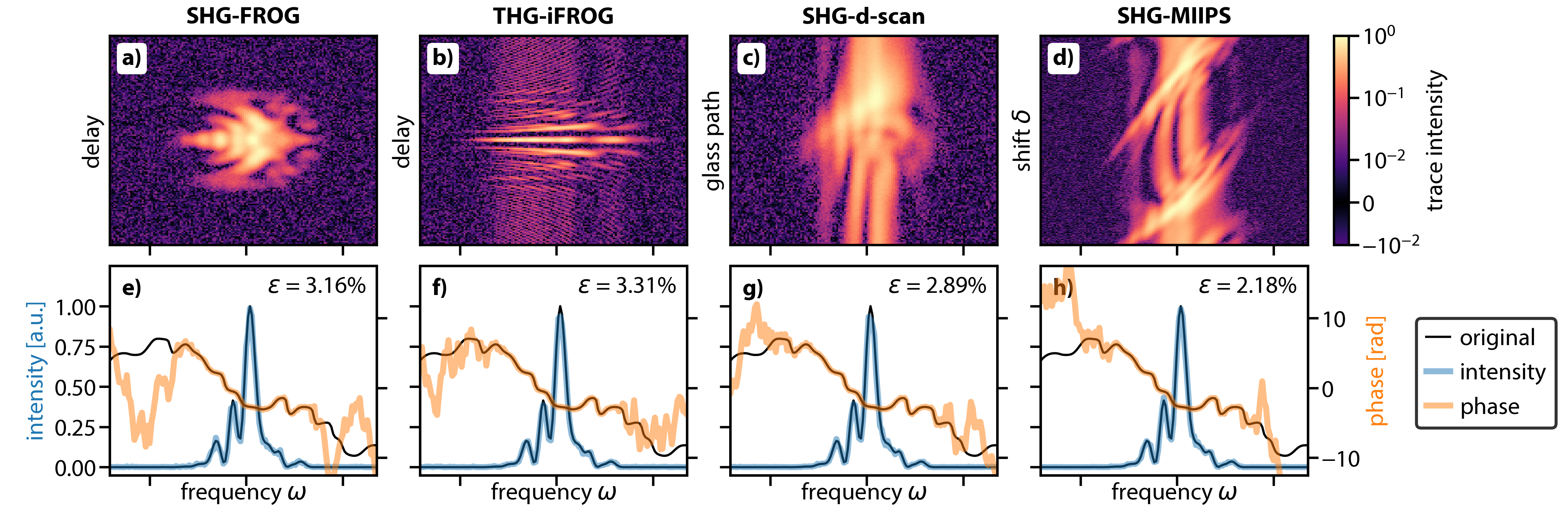
For illustration, four measurement traces with $\sigma=1\%$ and the pulses retrieved from them are shown in Fig. 3. In the following we will discuss the results in detail.

Convergence speed

Figure 4: Convergence behavior for $\sigma=0\%$. a) comparison of algorithms, b-d) comparison of PNPS methods when retrieving with COPRA. Shown is the median (bold line) and the interquartile range (shaded area) of the running minimum of $R$. Only the local iteration was used in COPRA.

Figure 5: Convergence behavior for noisy measurements ($\sigma=1\%$). a) comparison of algorithms, b-d) comparison of PNPS methods when retrieving with COPRA (solid: local iteration, dashed: global iteration). Shown is the median (bold line) and the interquartile range (shaded area) of the running minimum of $R$.

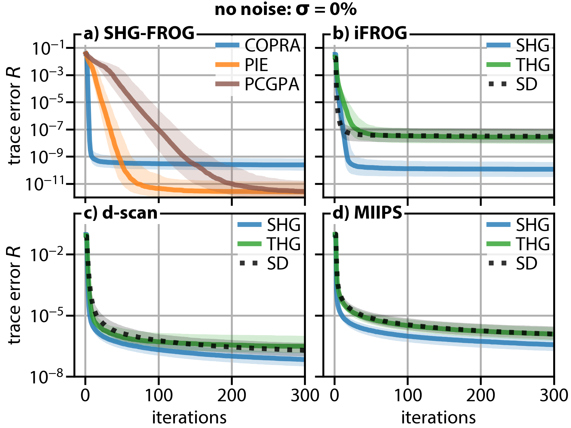
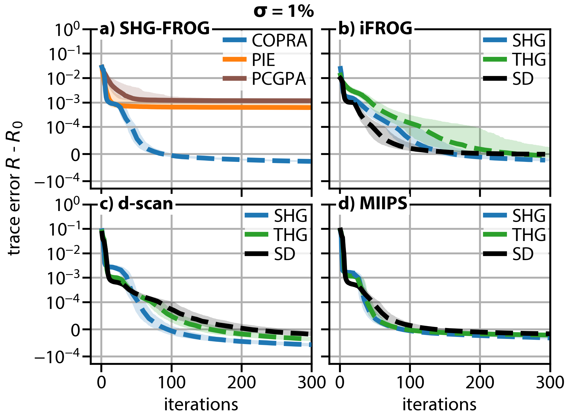
The typical convergence behavior of the local iteration for noiseless traces is shown in Fig. 4. It is important to note that the figures show the running minimum of the trace error, i.e., the best solution encountered. COPRA does not reduce the trace error in every step. For non-collinear schemes such as SHG-FROG we observed convergence to the accuracy limit of COPRA ($R\sim$110-9$$ for SHG) within just $20$ iterations, which is less than PCGPA and PIE require. For other PNPS schemes the initial convergence is just as fast, reaching the threshold of $R<$110-4$$ usually within tens of iterations.

For d-scan and MIIPS, especially for the variants using third-order nonlinearities, the convergence slows down at some point. We attribute this to the conditioning of the problem, which is known to directly affect the convergence speed of gradient descent methods [42]. However, usually this has no impact as stagnation sets in only below $R\sim$110-5$$ (see also Sec. 6.6.2).

The typical convergence behavior for noisy measurements is shown in Fig. 5. To quantify the convergence to the least-squares solution in this case the difference between the trace error $R$ and the trace error of the test pulse $R_{0}$ from (28) is used. The results demonstrate the role of the two stages in COPRA. The local iteration converges rapidly and then stagnates at roughly $R_{0}+$110-3$$. Afterwards, it is the global iteration that continues to minimize the squared sum of residuals $r$ and actually solves the pulse retrieval problem for noisy data in the least-squares sense.

In practice, COPRA converges very fast. For many PNPS measurements it finds a good solution with less than $100$ within iterations. For other PNPS methods a few hundred iterations are usually sufficient. Also, its actual run time compares favorably with other fast retrieval algorithms such as PCGPA and PIE and massively outperforms general minimization algorithms such as LM. For example, a single SHG-FROG retrieval with COPRA ($100$ iterations) on a grid with $N=256$ takes less than $3\text{\,}\mathrm{s}$ sec on a normal workstation. Furthermore, a single COBRA iteration requires only $5M$ to $7M$ 1D-FFTs with $N$ elements (depending on the scheme and the stage) and no operations with higher computational complexity. Hence, its computational complexity is approximately $MN\log N$.

Retrieval accuracy and retrieval probability

Figure 6: Robustness against additive Gaussian noise: a) synthetic SHG-FROG trace of a pulse with TBP 2. A high level of Gaussian noise was added ($\sigma=3\%$). b)-e) The pulses retrieved from the trace using different algorithms (blue: intensity, orange: phase) compared to the test pulse (black). $\varepsilon$ quantifies the retrieval accuracy.

Figure 7: The retrieval ratio (blue bar) and median retrieval error (inset number) of COPRA in dependence of the PNPS method and the noise level. A comparison with PCGPA and PIE for SHG-FROG is included. Successful retrieval was assumed if $R<R_{0}+$110-4$$.

In Fig. 5 we see that PCGPA and PIE do not achieve convergence in the least-squares sense. We found that, in general, no algorithm that incorporates the measurement trace solely by a projection has this property. This includes every algorithm based on generalized projections or the ptychographic engine. Both methods stagnate at roughly $R\sim R_{0}+$110-3$$ depending on the noise level – similar to the local iteration stage of COPRA.

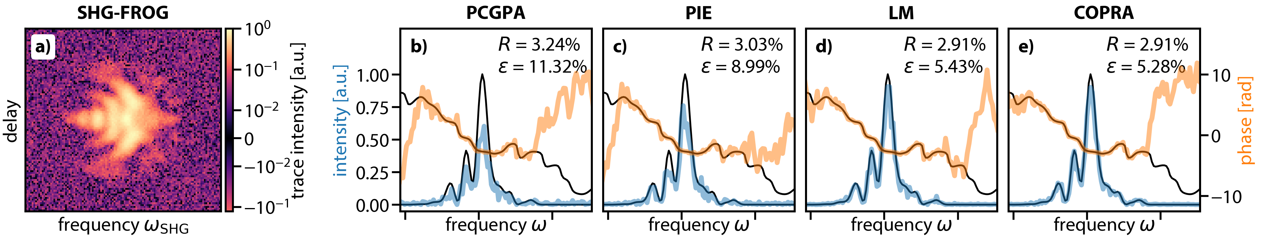
The impact of this can be seen in Fig. 6. It shows a comparison of the pulses retrieved from a very noisy SHG-FROG trace ($\sigma=3\%$) by using PCGPA, PIE, LM and COPRA. In each case the best solution after 10 runs of the algorithm is shown. The solutions obtained by PCGPA and PIE are clearly less accurate, having a retrieval error of $\varepsilon=11.32\%$ and $\varepsilon=8.99\%$ compared to $\varepsilon=5.43\%$ for COPRA. The pulse retrieved by LM confirms that COPRA does, in fact, obtain the least-squares solutions. At the same time one run of LM took $272\text{\,}\mathrm{s}$ to complete, compared to $7\text{\,}\mathrm{s}$ for COPRA.

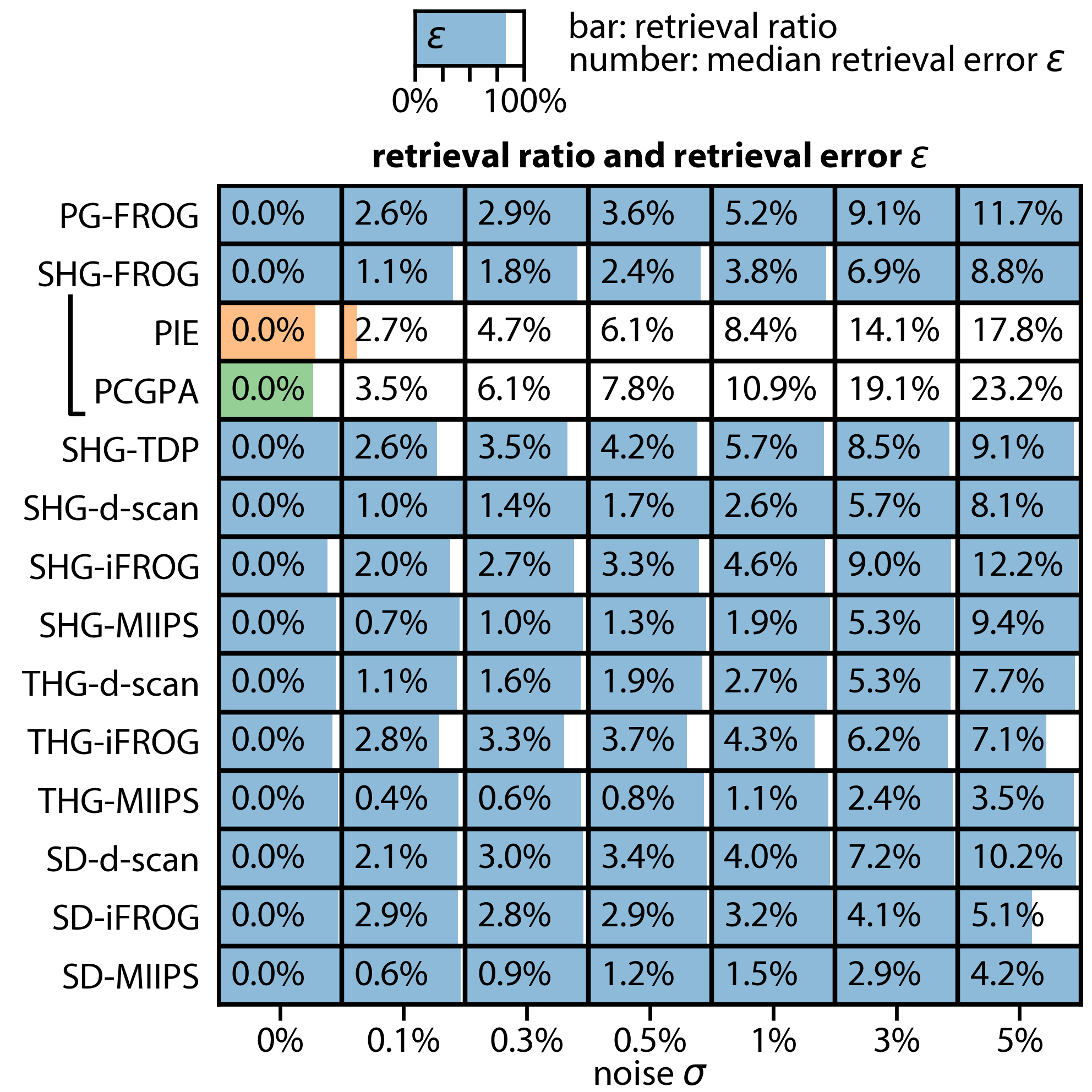
In Fig. 7 we show the retrieval ratio, i.e., the percentage of retrieved solutions that fulfill $R<R_{0}+$110-4$$, for all combinations of noise levels and PNPS schemes. The retrieval probability of COPRA is very high in all cases and usually above $90\%$. In practice a few repeated runs of COPRA from different initial guesses suffice. Also, we see that virtually none of the solutions obtained by PCGPA and PIE for noisy measurements fulfill our convergence criterion.

Additionally, Fig. 7 shows the retrieval errors achieved in the different cases. Shown is the median of the minimum retrieval error from $10$ runs achieved for each of the $100$ synthetic measurements. The results for SHG-FROG also show that PCGPA and PIE are less accurate than COPRA for all noise levels $\sigma>0\%$. This confirms the discussion from above.

We found that some PNPS schemes are more sensitive to noise and more susceptible to lack of convergence. E.g., SHG-iFROG measurements with $\sigma=1\%$ lead to $\varepsilon=4.5\%$ compared to $\varepsilon=2.6\%$ for SHG-d-scan. However, the actual dependence of $\varepsilon$ on the PNPS scheme, the trace error and the noise level is complex and a full description is out of scope for this work.

Uniqueness of the retrieved solutions

To verify the feasibility of the PNPS schemes as full pulse measurement methods we tested the uniqueness of the pulses retrieved by COPRA from noiseless, synthetic PNPS traces. To increase the search range we repeated the retrieval simulation starting COPRA from a random initial guess. Specifically, we searched for solutions of the retrieval problem that have a small trace error and simultaneously a large retrieval error, i.e., $R<$110-4$$ and $\varepsilon>1\%$. This would indicate the existence of a non-trivial ambiguity in one of these methods. To verify these solutions they were refined to high accuracy using the LM algorithm.

In this study we found no occurrence of an exact non-trivial ambiguity for any of the tested PNPS schemes. This is an indication that these measurements, in theory, define amplitude and phase of the pulse uniquely up to the trivial ambiguities. This includes MIIPS measurements, which to our knowledge have only been used for pulse compression so far.

However, we found that pulse retrieval from d-scan and MIIPS measurements may admit solutions with very low trace errors ($R\approx$110-5$$) that have additional weak satellite pulses at large delays. As those disappear after further refining of the solution to a level of $R<$110-9$$ the solutions do not constitute an ambiguity of the scheme in the strict sense. However, they will impact the retrieval from real, noisy measurements. This indicates that in general pulse retrieval from PNPS measurements should use some kind of regularization to select the correct solution. This can be done implicitly by starting COPRA with a temporally localized pulse, e.g., a Gaussian in the time domain. The satellite pulses only appeared as solutions for random initial guesses.

Notably COPRA performed well for many PNPS schemes even when using uninformed, random initial guesses. The retrieval ratio was mainly impacted for MIIPS measurements which admit several local solutions due to the periodicity of the applied phase patterns. The full results of the second retrieval simulation and further discussion of the satellite pulses in d-scan and MIIPS can be found in the supplementary material (Sec. S7).

6.3 Spectrally incomplete traces

Figure 8: Pulse retrieval from an incomplete THG-iFROG measurement. a) Synthetic measurement trace with added noise ($\sigma=1\%$). $25$ of $N=256$ spectral measurements were used for retrieval (indicated by color) b) The retrieved pulse (blue: intensity, orange: phase) and the test pulse (black). $\varepsilon$ quantifies the retrieval accuracy.

Sometimes it may be required to retrieve pulses from spectrally incomplete measurement traces. This may be due to, e.g., overlap with the fundamental spectrum or limitations of the spectrometer. The retrieval from spectrally incomplete traces was already demonstrated for d-scan and FROG [16, 33].

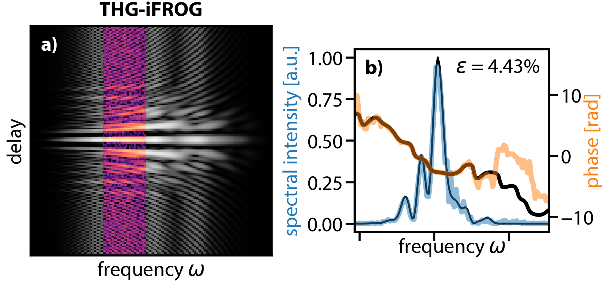
With small modifications COPRA can work with such traces. Mainly, Eqs. (14) and (22) have to be changed to include only the available $\omega_{n}$. Using this version of COPRA we found that retrieval from spectrally incomplete traces is possible for all PNPS schemes. Fig. 8 shows an example of an incomplete THG-iFROG measurement for which to our knowledge retrieval has not yet been demonstrated. The noisy measurement trace ($\sigma=1\%$) is the same as in Fig. 3 b) except that less than $10\%$ of the frequency range was selected (only $25$ spectral sampling points of $N=256$). Additionally, we included values of zero intensity in the measurement trace spanning the first and last $15\%$ of the simulation grid in frequency direction (not in the range shown in Fig. 8) which improved the retrieval accuracy by enforcing the localization of the pulse in the frequency domain. We can see that retrieval is possible with only a moderate loss of retrieval accuracy, i.e., the retrieval error is $\varepsilon=4.43\%$ compared to $\varepsilon=3.31\%$ for the complete trace from Fig. 3 b).

7 Conclusion

In conclusion, we showed that many self-referenced pulse measurement schemes are conceptually similar and can be described within a common mathematical framework. They measure the same quantity: sets of parametrized nonlinear process spectra (PNPS).

The PNPS pulse retrieval problem is naturally formulated as a nonlinear least-squares problem. Its solution is a maximum-likelihood estimate under the experimentally relevant assumption of Gaussian noise. This aspect was not fully appreciated before and methods that project on the measured intensity such as generalized projections and ptychography do not obtain a least-squares solution. Consequently, the accuracy of the retrieved solutions suffers unnecessarily in the presence of measurement noise.

The main result of the paper is the common pulse retrieval algorithm (COPRA), which can be directly applied to all PNPS measurements. We verified and demonstrated its capabilities numerically, by algorithmic testing of a large suite of synthetic PNPS traces generated from random pulses with increasing levels of noise. We found that COPRA is fast, robust, and accurate. It converges reliably onto the least-squares solution for all noise levels, even from fully random initial guesses. For noisy SHG-FROG measurements we compared COPRA to PCGPA and PIE and found COPRA to be far more accurate.

COPRA is universal and even applicable to PNPS measurements for which full amplitude and phase retrieval has not been shown before, e.g., MIIPS or SD-iFROG. Furthermore, COPRA is able to retrieve pulses from incomplete measurement traces, e.g., from iFROG traces with incomplete spectral sampling.

We anticipate that our algorithm will have great practical value. It was designed to be easy to implement and can be directly applied to a multitude of measurements. For FROG it does not impose any relation between the frequency and delay sampling, like it is required by PCGPA. For iFROG no calculation of a subtrace is necessary as COPRA works directly with the measurement data. For d-scan it offers a reliable and fast alternative to multi-dimensional optimization.

Some variants of COPRA remain subject of further work. For example, COPRA could be modified to work with XFROG and blind FROG. Simultaneous retrieval of the spectral response function of the measurement setup, like it was demonstrated for d-scan, could also be studied with COPRA.

Moreover, COPRA can be used as a universal and unbiased framework upon which the quality of a pulse measurement method may be judged. Which PNPS measurement is more suitable for a certain pulse can then be determined independently of the retrieval algorithm and solely based on the measurement method itself. COPRA may even be used to algorithmically engineer and optimize novel pulse retrieval methods.

In this sense, we hope that COPRA and the PNPS framework will help to give further insight in some fundamental questions of ultrashort pulse measurement: How much information is necessary for unique pulse retrieval? How large is the uncertainty in the retrieved pulse? Which PNPS method is most appropriate for certain kinds of pulses?

Funding

NCG acknowledges support by the German Federal Ministry of Education and Research under grant no 03ZZ0413 and grant no 03ZZ0467. TP acknowledges support by the German Research Foundation under grant no PE 1524/10-1. FE acknowledges support by the German Federal Ministry of Education and Research under grant no 13XP5053A.

Acknowledgement

NCG thanks JGG for providing the impetus to finally write up this manuscript.

See the supplementary material for supporting content.

References

- [1] I. A. Walmsley and C. Dorrer, “Characterization of ultrashort electromagnetic pulses,” \JournalTitleAdv. Opt. Photon. 1, 308–437 (2009).
- [2] E. P. Ippen and C. V. Shank, “Techniques for measurement,” in Ultrashort Light Pulses: Picosecond Techniques and Applications, S. L. Shapiro, ed. (Springer Berlin Heidelberg, 1977), pp. 83–122.
- [3] J.-C. M. Diels, J. J. Fontaine, I. C. McMichael, and F. Simoni, “Control and measurement of ultrashort pulse shapes (in amplitude and phase) with femtosecond accuracy,” \JournalTitleAppl. Opt. 24, 1270–1282 (1985).
- [4] J.-H. Chung and A. M. Weiner, “Ambiguity of ultrashort pulse shapes retrieved from the intensity autocorrelation and the power spectrum,” \JournalTitleIEEE Journal of Selected Topics in Quantum Electronics 7, 656–666 (2001).
- [5] D. J. Kane and R. Trebino, “Characterization of arbitrary femtosecond pulses using frequency-resolved optical gating,” \JournalTitleIEEE J. Quant. Electron. 29, 571–579 (1993).
- [6] R. Trebino, Frequency-Resolved Optical Gating: The Measurement of Ultrashort Laser Pulses (Springer US, 2000).
- [7] B. Seifert, H. Stolz, and M. Tasche, “Nontrivial ambiguities for blind frequency-resolved optical gating and the problem of uniqueness,” \JournalTitleJ. Opt. Soc. Am. B 21, 1089–1097 (2004).
- [8] T. Bendory, P. Sidorenko, and Y. C. Eldar, “On the uniqueness of FROG methods,” \JournalTitleIEEE Signal Processing Letters 24, 722–726 (2017).
- [9] G. Stibenz and G. Steinmeyer, “Interferometric frequency-resolved optical gating,” \JournalTitleOpt. Express 13, 2617–2626 (2005).
- [10] J. Hyyti, E. Escoto, and G. Steinmeyer, “Third-harmonic interferometric frequency-resolved optical gating,” \JournalTitleJ. Opt. Soc. Am. B 34, 2367–2375 (2017).
- [11] J. Hyyti, E. Escoto, and G. Steinmeyer, “Pulse retrieval algorithm for interferometric frequency-resolved optical gating based on differential evolution,” \JournalTitleReview of Scientific Instruments 88, 103102 (2017).
- [12] H. H. Bauschke and J. M. Borwein, “On projection algorithms for solving convex feasibility problems,” \JournalTitleSIAM Review 38, 367–426 (1996).
- [13] K. W. DeLong, B. Kohler, K. Wilson, D. N. Fittinghoff, and R. Trebino, “Pulse retrieval in frequency-resolved optical gating based on the method of generalized projections,” \JournalTitleOpt. Lett. 19, 2152–2154 (1994).
- [14] D. J. Kane, G. Rodriguez, A. J. Taylor, and T. S. Clement, “Simultaneous measurement of two ultrashort laser pulses from a single spectrogram in a single shot,” \JournalTitleJ. Opt. Soc. Am. B 14, 935–943 (1997).
- [15] M. Miranda, T. Fordell, C. Arnold, A. L’Huillier, and H. Crespo, “Simultaneous compression and characterization of ultrashort laser pulses using chirped mirrors and glass wedges,” \JournalTitleOpt. Express 20, 688–697 (2012).
- [16] M. Miranda, C. L. Arnold, T. Fordell, F. Silva, B. Alonso, R. Weigand, A. L’Huillier, and H. Crespo, “Characterization of broadband few-cycle laser pulses with the d-scan technique,” \JournalTitleOpt. Express 20, 18732–18743 (2012).
- [17] M. Hoffmann, T. Nagy, T. Willemsen, M. Jupé, D. Ristau, and U. Morgner, “Pulse characterization by THG d-scan in absorbing nonlinear media,” \JournalTitleOpt. Express 22, 5234–5240 (2014).
- [18] M. Canhota, F. Silva, R. Weigand, and H. M. Crespo, “Inline self-diffraction dispersion-scan of over octave-spanning pulses in the single-cycle regime,” \JournalTitleOpt. Lett. 42, 3048–3051 (2017).
- [19] M. Miranda, J. Penedones, C. Guo, A. Harth, M. Louisy, L. Neoričić, A. L’Huillier, and C. L. Arnold, “Fast iterative retrieval algorithm for ultrashort pulse characterization using dispersion scans,” \JournalTitleJ. Opt. Soc. Am. B 34, 190–197 (2017).
- [20] V. V. Lozovoy, I. Pastirk, and M. Dantus, “Multiphoton intrapulse interference. IV. Ultrashort laser pulse spectral phase characterization and compensation,” \JournalTitleOpt. Lett. 29, 775–777 (2004).
- [21] B. Xu, J. M. Gunn, J. M. D. Cruz, V. V. Lozovoy, and M. Dantus, “Quantitative investigation of the multiphoton intrapulse interference phase scan method for simultaneous phase measurement and compensation of femtosecond laser pulses,” \JournalTitleJ. Opt. Soc. Am. B 23, 750–759 (2006).
- [22] A. Galler and T. Feurer, “Pulse shaper assisted short laser pulse characterization,” \JournalTitleApplied Physics B 90, 427–430 (2008).
- [23] N. Forget, V. Crozatier, and T. Oksenhendler, “Pulse-measurement techniques using a single amplitude and phase spectral shaper,” \JournalTitleJ. Opt. Soc. Am. B 27, 742–756 (2010).
- [24] V. Loriot, G. Gitzinger, and N. Forget, “Self-referenced characterization of femtosecond laser pulses by chirp scan,” \JournalTitleOpt. Express 21, 24879–24893 (2013).
- [25] D. E. Wilcox and J. P. Ogilvie, “Comparison of pulse compression methods using only a pulse shaper,” \JournalTitleJ. Opt. Soc. Am. B 31, 1544–1554 (2014).
- [26] D. Spangenberg, E. Rohwer, M. H. Brügmann, and T. Feurer, “Ptychographic ultrafast pulse reconstruction,” \JournalTitleOpt. Lett. 40, 1002–1005 (2015).
- [27] D.-M. Spangenberg, M. Brügmann, E. Rohwer, and T. Feurer, “All-optical implementation of a time-domain ptychographic pulse reconstruction setup,” \JournalTitleAppl. Opt. 55, 5008–5013 (2016).
- [28] T. Witting, D. Greening, D. Walke, P. Matia-Hernando, T. Barillot, J. P. Marangos, and J. W. G. Tisch, “Time-domain ptychography of over-octave-spanning laser pulses in the single-cycle regime,” \JournalTitleOpt. Lett. 41, 4218–4221 (2016).
- [29] R. Hegerl and W. Hoppe, “Dynamische Theorie der Kristallstrukturanalyse durch Elektronenbeugung im inhomogenen Primärstrahlwellenfeld,” \JournalTitleBerichte der Bunsengesellschaft für physikalische Chemie 74, 1148–1154 (1970).
- [30] A. M. Maiden and J. M. Rodenburg, “An improved ptychographical phase retrieval algorithm for diffractive imaging,” \JournalTitleUltramicroscopy 109, 1256–1262 (2009).
- [31] A. Maiden, D. Johnson, and P. Li, “Further improvements to the ptychographical iterative engine,” \JournalTitleOptica 4, 736–745 (2017).
- [32] A. M. Heidt, D.-M. Spangenberg, M. Brügmann, E. G. Rohwer, and T. Feurer, “Improved retrieval of complex supercontinuum pulses from XFROG traces using a ptychographic algorithm,” \JournalTitleOpt. Lett. 41, 4903–4906 (2016).
- [33] P. Sidorenko, O. Lahav, Z. Avnat, and O. Cohen, “Ptychographic reconstruction algorithm for frequency-resolved optical gating: super-resolution and supreme robustness,” \JournalTitleOptica 3, 1320–1330 (2016).
- [34] P. Sidorenko, O. Lahav, Z. Avnat, and O. Cohen, “Ptychographic reconstruction algorithm for frequency resolved optical gating: super-resolution and extreme robustness: erratum,” \JournalTitleOptica 4, 1388–1389 (2017).
- [35] C. Iaconis and I. A. Walmsley, “Spectral phase interferometry for direct electric-field reconstruction of ultrashort optical pulses,” \JournalTitleOpt. Lett. 23, 792–794 (1998).
- [36] D. Keusters, H.-S. Tan, P. O’Shea, E. Zeek, R. Trebino, and W. S. Warren, “Relative-phase ambiguities in measurements of ultrashort pulses with well-separated multiple frequency components,” \JournalTitleJ. Opt. Soc. Am. B 20, 2226–2237 (2003).
- [37] T. Bendory, R. Beinert, and Y. C. Eldar, “Fourier phase retrieval: Uniqueness and algorithms,” in Compressed Sensing and its Applications, H. Boche, G. Caire, R. Calderbank, M. März, G. Kutyniok, and R. Mathar, eds. (Birkhäuser, 2017), pp. 55–91.
- [38] A. Tarantola, Inverse problem theory and methods for model parameter estimation (SIAM, 2005).
- [39] G. Seber and C. Wild, Nonlinear Regression (Wiley, 2003).
- [40] J. J. Davenport, J. Hodgkinson, J. R. Saffell, and R. P. Tatam, “Noise analysis for CCD-based ultraviolet and visible spectrophotometry,” \JournalTitleAppl. Opt. 54, 8135–8144 (2015).
- [41] E. Escoto, A. Tajalli, T. Nagy, and G. Steinmeyer, “Advanced phase retrieval for dispersion scan: a comparative study,” \JournalTitleJ. Opt. Soc. Am. B 35, 8–19 (2018).
- [42] J. Nocedal and S. J. Wright, Numerical Optimization (Springer, 2006), 2nd ed.