Rapid buildup of a magnetic flux rope during a confined X2.2 class flare in NOAA AR 12673

Abstract

Magnetic flux ropes (MFRs) are believed to be the core structure in solar eruptions, nevertheless, their formation remains intensely debated. Here we report a rapid buildup process of an MFR-system during a confined X2.2 class flare occurred on 2017 September 6 in NOAA AR 12673, three hours after which the structure erupted to a major coronal mass ejection (CME) accompanied by an X9.3 class flare. For the X2.2 flare, we do not find EUV dimmings, separation of its flare ribbons, or clear CME signatures, suggesting a confined flare. For the X9.3 flare, large-scale dimmings, separation of its flare ribbons, and a CME show it to be eruptive. By performing a time sequence of nonlinear force-free fields (NLFFFs) extrapolations we find that: until the eruptive flare, an MFR-system was located in the AR. During the confined flare, the axial flux and the lower bound of the magnetic helicity for the MFR-system were dramatically enhanced by about $86\%$ and $260\%$, respectively, although the mean twist number was almost unchanged. During the eruptive flare, the three parameters were all significantly reduced. The results evidence the buildup and release of the MFR-system during the confined and the eruptive flare, respectively. The former may be achieved by flare reconnection. We also calculate the pre-flare distributions of the decay index above the main polarity inversion line (PIL) and find no significant difference. It indicates that the buildup of the magnetic flux and helicity of the MFR-system may play a role in facilitating its final eruption.

1 INTRODUCTION

Magnetic flux ropes, consisting of twisted field lines winding around the main axis, are fundamental structures on the sun. It’s generally accepted that the main drivers of hazardous space weather - CMEs - are expulsions of MFRs (e.g., Amari et al. 2000, Cheng et al. 2017). Therefore, their properties, e.g., formation, evolution, stability, are long-standing topics. In most solar eruption models, the MFRs play key roles. In some ideal magnetohydrodynamic (MHD) models, pre-existing MFRs are required: once the background magnetic fields decrease fast enough (torus instability, Kliem & Török 2006), or the rope’s twist number reaches a critical value (kink instability, Török et al. 2004), the eruption happens. In some non-ideal models, MFRs can be formed during the eruption: magnetic reconnection happens below (tether-cutting model, Moore et al. 2001) or above (breakout model, Antiochos et al. 1999) the sheared magnetic arcades, then forms the MFR and initiates the eruption. In either kind of models, the eruption entity is the MFR.

Despite its pre-existence for an eruption, the MFR is proposed to be formed or strengthened mainly through two ways: one is its bodily emergence, supported by simulations (e.g., Fan 2001, Leake et al. 2013) and observations (e.g., Okamoto et al. 2008), though questioned by some work (Vargas Domínguez et al. 2012); the other is reconnection mechanism, in which the MFR is formed/strengthened through the reconnection (e.g., Cheng et al. 2011, Zhang et al. 2012, Wang et al. 2017), sometimes manifested as flux cancellation (e.g., Green et al. 2011). The twist numbers of interplanetary MFRs are usually larger than that of pre-eruption MFRs, suggesting that the latter may be strengthened by reconnection during the eruptions (Wang et al. 2016). Besides, photospheric flows/motions, e.g., shear/converging motions, sunspot rotations are reported to build up the MFRs effectively (e.g., Fan 2009, Yan et al. 2018).

In the reconnection formation scenario, the MFRs can even be formed during confined flares before successful eruptions as reported: Patsourakos et al. (2013) observed a limb event, showing the formation of an MFR during a confined C4.5 GOES class flare before its ejection in the subsequent M7.7 flare; Guo et al. (2013) suggested that an MFR can be built-up during a series of confined flares before a CME and a major flare; Chintzoglou et al. (2015) reported formation and strengthening of two MFRs during confined flares before two successive CMEs; James et al. (2018) also reported an MFR formation in a confined flare before its final eruption.

Nevertheless, the formation/buildup of MFRs during as intense as X-class flares is barely reported to our best knowledge. Here we present a buildup process of an MFR-system during a confined X2.2 flare (SOL2017-09-06T08:57) that occurred in NOAA active region (AR) 12673, which erupted to a major CME accompanied by an X9.3 flare (SOL2017-09-06T11:53) three hours later. We mainly focus on analyzing the properties of the source coronal magnetic fields (CMFs) based on a time-sequence of NLFFF extrapolations.

2 Data and Methods

Both analyzed flares occurred near S09W33. Their on-disk evolution is captured by SDO/AIA (Pesnell et al. 2012). The associated coronal outflows are observed by SOHO/LASCO (Domingo et al. 1995). The photospheric vector magnetic fields are recorded by SDO/HMI. Here a magnetic-field data product called SHARP (Bobra et al. 2014) is used. The three dimensional CMFs are reconstructed by an NLFFF extrapolation model (Wiegelmann 2004, Wiegelmann et al. 2012) and a potential fields (PFs) model (e.g., Sakurai 1989), using SHARP magnetograms as the bottom boundaries.

Based on the reconstructed CMFs, we may identify the MFR by combining the twist number $T_{w}$ and squashing factor $Q$ (Liu et al. 2016). $T_{w}$ measures the number of turns of a field line winding, and is calculated by $\displaystyle T_{w}=\frac{1}{4\pi}\int_{l}\alpha dl$. $\alpha$, $l$ and $dl$ denote the force-free parameter, the field line length, and the elementary length, respectively. $Q$ measures the change of the connectivity of the field lines. High $Q$ values indicate the positions of quasi-separatrix layers (QSLs) where the connectivity changes dramatically (e.g., Démoulin et al. 1996). For an MFR, its twisted fields lines are distinct from the surrounding fields, thus are wrapped by QSL. Its cross section displays a twisted region enclosed by high $Q$ lines.

Once the MFR is located, its toroidal (i.e., axial) flux can be calculated by $\Phi_{t}=\bf{B}\cdot\bf{S}$, where ${\bf S}=S\bf{n}$, $S$ and $\bf{n}$ denote the area and normal unit vector of its cross section. The flux-weighted mean twist number can be computed by $\displaystyle<|T_{w}|>=\frac{\Sigma|T_{w}B_{n}|dA}{\Sigma|B_{n}|dA}$, where $dA$ is the elementary area. Its magnetic helicity can be simply estimated by a twist number method (Priest & Forbes 2000, Guo et al. 2013, Yang et al. 2016, Guo et al. 2017) using $H_{twist}\approx T_{w}\Phi^{2}$. Magnetic helicity measures the geometrical complexity of the magnetic fields. For a single MFR, the aforementioned method is applicable when its writhe can be omitted, giving the lower bound of its helicity.

Additionally, the decay index measuring the decrease of the external PFs with height can be calculated by $\displaystyle n=-\frac{\rm\partial\,\ln B_{ex}(h)}{\rm\partial\,\ln h}$. $B_{ex}$ is the traverse component of PFs and $h$ is the height. As stated in torus instability theory, the background PFs play the major role in confining the eruption. Once the MFR reaches a region where $n$ is beyond a threshold, the torus instability will occur. The threshold value varies depending on the properties of the MFR (e.g., Démoulin & Aulanier 2010, Olmedo & Zhang 2010). We use 1.5 (Kliem & Török 2006) as a representative value here.

3 Observation and Analysis

3.1 Eruptiveness of the Flares

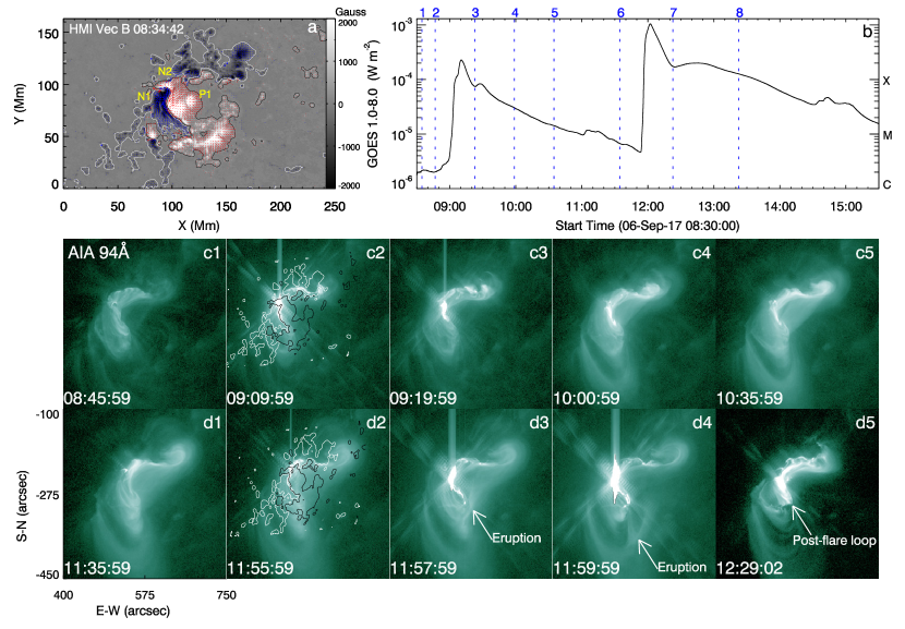
Figure 1: a: Photospheric magnetic fields of the AR. The background shows the vertical fields ($B_{z}$). N1 (P1, N2) refers to the main negative (main positive, northern negative) polarity. White (black) contours outline $B_{z}$ at -150 (150) Gauss (same in c2 and d2). The arrows refer to the horizontal fields ($B_{h}$). b: GOES 1–8 Å flux. The blue-dashed lines 1–8 indicate the instances used in Section 3.2. c1–c5 (d1–d5): Snapshots of the first (second) flare observed in 94 Å.

NOAA AR 12673 exhibited the fastest magnetic flux emergence ever observed at its early stage (Sun & Norton 2017), and had been relatively well-developed when producing the two flares (Figure 1a). The source of both flares involved the central main polarities (N1 and P1) and the northern negative polarity (N2). Before both flares, hot channels (HCs), which refer to the S-shaped structures appearing above the PILs in high-temperature AIA passbands (94 and 131 Å) and considered as the proxies of MFRs (e.g., Zhang et al. 2012), were visible in 94 Å (Figure 1c1 and d1). Although the one before the first flare was slightly diffuse, the HCs indicated the existence of MFRs. During the first flare, brightenings occurred along the HC, after which an HC was still found (Figure 1c2–c5). During the second flare, the eruption of the HC was observed; post-flare loops appeared later (Figure 1d2–d5). The observations hint that the first (second) flare may be confined (eruptive).

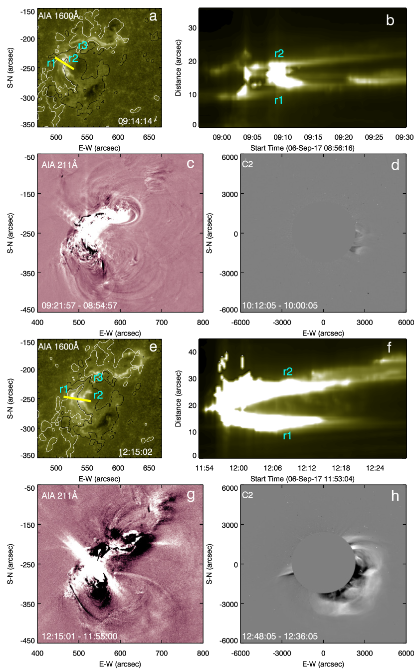
Figure 2: a–d: Details of the first flare. a: Flare ribbons in 1600 Å. Contours outline $B_{z}$. The letters r1 (r2, r3) denotes the ribbon in the polarity N1 (P1, N2). b: Time-distance plot of a slice (yellow line in a). c: Base-difference image at the 211 Å passband. d: Coronal outflow observed by LASCO/C2. e–h: Similar layouts as a–d but for the second flare. An animation, including the GOES 1–8 Å flux, $B_{z}$, observations in 1600, 304, 211, 94 Å and the coronagraph is available online.

In both flares, three ribbons (r1, r2 and r3 in Figure 2) appeared in 1600 Å passband. For the first flare, the two main ribbons (r1 and r2) did not separate as a function of time (Figure 2b), which is in contrast to that of an eruptive flare as stated in standard flare model (e.g., Carmichael 1964), also indicating a confined flare. No large-scale dimmings were observed in 211 Å (Figure 2c). Careful inspection of the observations in 304 Å neither finds ejection signs. The associated faint and narrow coronal outflow (Figure 2d) might not be enough to be defined as a CME. For the second flare, Figure 2f clearly shows that the ribbons separated as the flare evolved. Clear dimmings were seen in 211 Å passband after the flare (Figure 2g), indicating mass depletion. The appeared bright, halo CME (Figure 2h) further confirmed the second flare being eruptive.

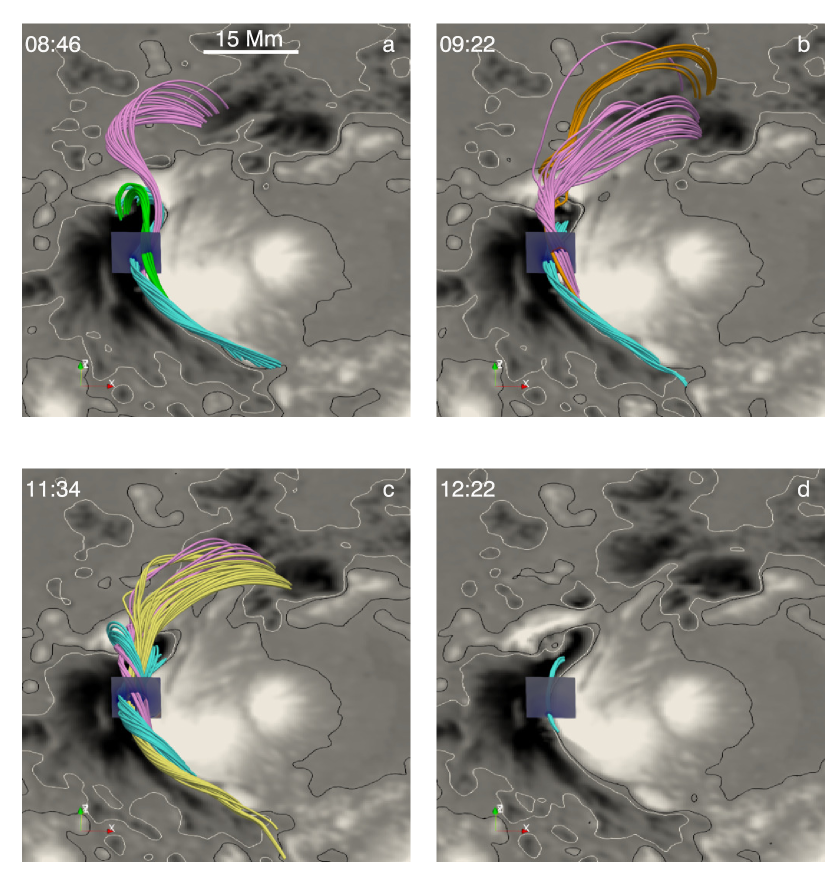
Figure 3: a–b (c–d): Representative field lines of the core structure above the PIL before and after the confined (eruptive) flare, showing an MFR-system in a–c and a sheared structure in d. Different colors represent different branches. The backgrounds are $B_{z}$. The vertical planes mark the position of the plane used in Figure 4.

We calculate $T_{w}$ and $Q$ in multiple vertical planes across the main PIL to trace the possible MFR before and after the flares (see details in Section 3.2). The selected field lines tracing through twisted/highly sheared regions enclosed by high $Q$ lines are shown in Figure 3. Before the confined flare, an MFR-like structure composed of different branches of field lines was located (Figure 3a). Two branches connected N1 and P1 (cyan and green lines), having distinguishable boundaries in the $T_{w}$ and $Q$ maps (see Section 3.2). One branch (magenta lines) connected P1 and N2. The footpoints of the field lines corresponded to the positions of the flare ribbons. Note that, a mature MFR requires its field lines having a coherent structure, which wasn’t perfectly met here. However, the branches were located close, evolved as a whole and erupted together finally (see contents below). Thus, we name the structure an MFR-system. After the confined flare, an MFR-system was also found (Figure 3b), although its configuration was significantly different from the one before the flare. It was still composed of different branches, with one branch connecting N1 and P1 (cyan lines), two branches connecting P1 and N2 with opposite handedness (magenta and brown lines in Figure 3b, see section 3.2). The survival of the MFR-system was consistent with the absence of a CME.

Before the eruptive flare, an MFR-system was still located (Figure 3c), though its topology had a slight change, appearing longer field lines (shown in yellow). The footpoints of these field lines were consistent with the positions of the flare ribbons. After the flare, the MFR-system disappeared, only a sheared structure survived (Figure 3d).

In summary, for the X2.2 flare, no clear EUV dimmings or separation of its flare ribbons were observed; the accompanied coronal outflow was faint and narrow, indicating a confined flare. For the X9.3 flare, clear on-disk eruption signs, EUV dimmings, separation of its flare ribbons, and the accompanied major CME indicated an eruptive flare. The survival and disappearance of the MFR-system after respective flare were consistent with their eruptiveness.

3.2 Buildup of the MFR-system during the Confined Flare

3.2.1 Boundary of the MFR-system

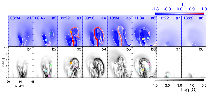
Figure 4: The upper (lower) row: $T_{w}$ ($Q$) maps in a plane across the core structure, which is an MFR-system in 1–6 and a sheared structure in 7–8. Panels 1–8 correspond to the instances 1–8 marked in Figure 1b. $\times$ symbols in 2, 3, 6 and 7 mark the representative positions of different rope branches, corresponding to the field lines in Figure 3. The white dots in the upper row outline the boundaries of the core structure.

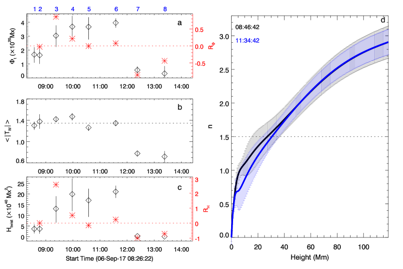
Figure 5: a: Temporal evolution of $\Phi_{t}$ and its fractional change $R_{\Phi}$. b: Evolution of $<|T_{w}|>$. The horizontal-dashed line indicates its median value (1.35 turns). c: Evolution of $H_{twist}$. d: Pre-flare distributions of $n$ above the PIL. Each data point is the average at this height. The errors are the standard deviations.

To quantitatively study the properties of the MFR-system, we select eight instances (vertical-dashed lines in Figure 1b), at which $T_{w}$ and $Q$ distributions in a vertical plane are displayed (Figure 4). We choose the plane because it intersected all rope branches. The computational grid of the plane is refined by 16 times for a higher precision (following Liu et al. 2016). To additionally calculate $\Phi_{t}$, $<|T_{w}|>$, and $H_{twist}$ of the MFR-system, its boundary needs to be determined. Owing to that perfectly closed QSLs enclosing the MFR-system cannot be found here, the boundaries (white dotted-lines in Figure 4) are determined manually through combining the high-$Q$ lines and contours of the thresholds of $|T_{w}|$. The thresholds are decided when the high $Q$ and contour lines connect smoothly, resulting in a value of 1.1 before the eruptive flare (1-6 in Figure 4), and 0.7 after the eruptive flare (7-8 in Figure 4). The parameters calculated in the cross sections are shown in Figure 5. The fractional changes of $\Phi_{t}$ and $H_{twist}$ are calculated by $\displaystyle R_{\Phi}=\frac{\Phi_{t}(i)-\Phi_{t}(i-1)}{\Phi_{t}(i-1)}$ and $\displaystyle R_{H}=\frac{H_{twist}(i)-H_{twist}(i-1)}{H_{twist}(i-1)}$, respectively, $i$ means the $i_{th}$ instance.

Uncertainty for each parameter is considered from two sources: the selection of the plane and the determination of the MFR-system boundaries. For the former, we choose another two planes that also intersected all rope branches and repeat the calculation, then regard the standard deviation of the values from the three planes as part of the upper/lower error shown in Figure 5. For the later, we apply the morphological erosion and dilation, with a circular kernel ($r\approx 0.1$ Mm), to the regions in the determined boundaries, resulting in a shrunken and a distend regions where we calculate the parameter again; the difference between the values from the original and the distend (shrunken) regions is regarded as the other part of the upper (lower) error. The final errors shown in Figure 5 are the sum of the two parts.

3.2.2 Evolution of the Properties of the MFR-system

At the two instances (1 and 2 in Figure 4) before the confined flare, $T_{w}$ and $Q$ maps showed no significant change. Three twisted regions ($\times$ symbols in Figure 4a2, 4b2) with distinguishable $Q$ boundaries were located, confirming the existence of an MFR-system with different branches, as shown in Figure 3a. After the first flare, twisted regions with high $Q$ boundaries can still be found (3 in Figure 4), consistent with the MFR-system shown in Figure 3b. The right part of the twisted regions showed a field lines set with left handedness (negative twist) overlain by another set with right handedness (positive twist), displaying a complex configuration. The cross section of the structure displayed an apparent expansion. Its equivalent radius increased from 1.6 Mm to 2.6 Mm, indicating a possible enhancement of the axial flux. Meanwhile, its estimated length ($\sim$100 Mm) and height (below 10 Mm) didn’t change significantly.

At the instances between the two flares (4, 5 and 6 in Figure 4), twisted regions with high $Q$ lines were all located, although with their patterns slightly changing, indicating that the MFR-system was evolving slowly. After the eruptive flare (7 in Figure 4), the twisted region disappeared, left a strongly sheared region (with average $|T_{w}|$ around 0.8 turns), consistent with the eruption of the observed HC. One hour later, a sheared structure was still located, having lower $T_{w}$ ($\sim$ 0.6) and smaller cross section (8 in Figure 4).

The temporal evolution of $\Phi_{t}$ (Figure 5a) showed that it experienced a dramatic increase after the confined flare from $1.63\times 10^{20}$ Mx to $3.04\times 10^{20}$ Mx (by $86\%$), then increased slowly to $3.96\times 10^{20}$ Mx at 11:34 UT, and finally reduced to $0.56\times 10^{20}$ Mx after the eruptive flare. In the mean time, $<|T_{w}|>$ kept a value around 1.3 and dropped to 0.8 before and after the eruptive flare, respectively (Figure 5b). $H_{twist}$ also dramatically increased from $3.7\times 10^{40}$ Mx² to $13.1\times 10^{40}$ Mx² (by $260\%$) after the confined flare, then slowly evolved to $21.1\times 10^{40}$ Mx² at 11:34 UT, and decreased to $0.2\times 10^{40}$ Mx² after the eruptive flare (Figure 5c). Moreover, as the decay index distributions in Figure 5d showed, before both flares, $n$ reached the critical height (where $n=1.5$) around 30 Mm, showing no significant difference when considering the computing errors.

The magnetic flux and helicity of the entire AR were also estimated. The former was on the order of $\sim 10^{22}$ Mx. The latter was an accumulated value since the emergence of the AR, and was roughly assessed based on a velocity estimation method called DAVE4VM (Schuck 2008); its value was on the order of $\sim 10^{43}$ Mx². The two parameters of the MFR-system only accounted for $\sim 1\%$ of the values of the AR.

In summary, we calculate $T_{w}$ and $Q$ in the cross section of the MFR-system at eight instances, and analyze the evolution of its $\Phi_{t}$, $<|T_{w}|>$, and $H_{twist}$. During the confined flare, the twist number had no significant change; interestingly, its axial flux and magnetic helicity were enhanced dramatically. After the eruptive flare, the parameters were all significantly reduced. The results indicate a rapid buildup and a release process of the MFR-system during the confined and eruptive flare, respectively. The similar pre-flare distributions of the decay index further suggest that the change of the MFR-system itself may play a more significant role in its final eruption here.

4 Summary and Discussions

Here we present a buildup process of an MFR-system during a confined X2.2 flare occurred on 2017 September 6 in NOAA AR 12673, which was evidenced by significant enhancement of its axial flux and magnetic helicity. The MFR-system erupted to a major CME during the following X9.3 flare three hours later.

Note that, the coronal outflow associated with the first flare is classified as a CME in some work (e.g., Yan et al. 2018). However, it was very faint, narrow, and did not propagate further than 10 $R_{\odot}$, being clearly different from the major CME associated with the second flare. This kind of outflows, showing no clear shape of MFRs, failing to propagate to a large distance that seem not to be related to MFRs, are defined as “pseudo-” CMEs (Vourlidas et al. 2010, 2013). The outflow here should not be relevant to the MFR-system we discussed. Combined with the evidence in Section 3.1, we argue that the X2.2 flare was confined. Verma (2018) also found localized, confined flare kernels in white-light emission of the X2.2 flare and separating ribbons in that of the X9.3 flare, consistent with our arguments.

The structure composed of multiple field lines branches here was defined as an MFR-system. Note that, we cannot exclude the possibility that those branches were different MFRs due to the distinguishable boundaries they had, and the opposite helicity signs that different branches further displayed after the first flare. However, the branches were located close; more importantly, they evolved and erupted together, indicating that defining the structure as an MFR-system should be reasonable. The QSL of the MFR-system was not perfectly closed, indicating a possible bald patch topology (e.g., Savcheva et al. 2012), and/or ongoing development. The evolution of $Q$ and $T_{w}$ patterns supported its development. When no eruption occurred, the slow evolution of the MFR-system may be driven by sunspot rotation and shear motion (Yan et al. 2018). The multiple-branch configuration of an MFR-system has been reported (Inoue et al. 2016, e.g.,, Cheng et al. 2014, or double-decker MFR in e.g.,), and is thought to play a role in an eruption when interaction exists between different branches (Awasthi et al. 2018).

Besides the final eruption, the most dramatic change of the MFR-system happened during the confined flare. Its axial flux and magnetic helicity increased by $86\%$ and $260\%$ within tens of minutes, clearly evidencing a rapid buildup of the MFR-system. The process can be achieved by the fast flare reconnection, which can add flux to a pre-existing MFR efficiently. Here the reconnection may start at the QSL between different branches, involving not only the rope fields but also the surrounding fields, adding more flux to the rope. Correspondence between the footpoints of the MFR-system and the flare ribbons also supported such a scenario. The mean twist number did not significantly change during the confined flare, indicating that the toroidal and poloidal flux were added to the MFR-system with equal proportion, keeping the twist number relatively invariant. Meanwhile, the decay index distributions showed no significant evolution. The result was in agreement with Nindos et al. (2012), in which small temporal evolution of the decay index, accompanied by helicity buildup, was found during a multi-day period when various eruptive and non-eruptive flares occurred.

The increase of the MFR-system flux may lead to a easier catastrophe (e.g., Zhang et al. 2016). The enhanced magnetic helicity of the MFR-system is related to the helicity of the current-carrying magnetic fields, the ratio of which to the total helicity is positively correlated to the CME eruptivity of a region (Pariat et al. 2017). Based on the fact of nearly invariant decay index, we conjecture that the first confined flare enhanced the MFR-system so that facilitated the next successful eruption. The result is also consistent with a so-called “domino-effect” scenario (Zuccarello et al. 2009), which emphasizes the influence from the previous activity. One should pay more attention to the close precursors of the eruptions (Wang et al. 2013, Liu et al. 2017), since they might play roles in facilitating the final eruptions.

References

- Amari et al. (2000) Amari, T., Luciani, J. F., Mikic, Z., & Linker, J. 2000, The Astrophysical Journal, 529, L49
- Antiochos et al. (1999) Antiochos, S. K., DeVore, C. R., & Klimchuk, J. a. 1999, The Astrophysical Journal, 510, 485
- Awasthi et al. (2018) Awasthi, A. K., Liu, R., Wang, H., Wang, Y., & Shen, C. 2018, The Astrophysical Journal, 857, 124
- Bobra et al. (2014) Bobra, M. G., Sun, X., Hoeksema, J. T., et al. 2014, Solar Physics, 289, 3549
- Carmichael (1964) Carmichael, H. 1964, NASA Special Publication, 50, 451
- Cheng et al. (2014) Cheng, X., Ding, M. D., Zhang, J., et al. 2014, The Astrophysical Journal, 789, 93
- Cheng et al. (2017) Cheng, X., Guo, Y., & Ding, M. 2017, Science China Earth Sciences, 60, 1383
- Cheng et al. (2011) Cheng, X., Zhang, J., Liu, Y., & Ding, M. D. 2011, The Astrophysical Journal, 732, L25
- Chintzoglou et al. (2015) Chintzoglou, G., Patsourakos, S., & Vourlidas, A. 2015, Astrophys. J., 809, 34
- Démoulin & Aulanier (2010) Démoulin, P., & Aulanier, G. 2010, The Astrophysical Journal, 718, 1388
- Démoulin et al. (1996) Démoulin, P., Hénoux, J. C., Priest, E. R., & Mandrini, C. H. 1996, Astronomy and Astrophysics, 308, 643
- Domingo et al. (1995) Domingo, V., Fleck, B., & Poland, A. I. 1995, Solar Physics, 162, 1
- Fan (2001) Fan, Y. 2001, The Astrophysical Journal, 554, L111
- Fan (2009) —. 2009, The Astrophysical Journal, 697, 1529
- Green et al. (2011) Green, L. M., Kliem, B., & Wallace, A. J. 2011, Astronomy & Astrophysics, 526, A2
- Guo et al. (2013) Guo, Y., Ding, M. D., Cheng, X., Zhao, J., & Pariat, E. 2013, The Astrophysical Journal, 779, 157
- Guo et al. (2017) Guo, Y., Pariat, E., Valori, G., et al. 2017, The Astrophysical Journal, 840, 40
- Inoue et al. (2016) Inoue, S., Hayashi, K., & Kusano, K. 2016, The Astrophysical Journal, 818, 168
- James et al. (2018) James, A. W., Valori, G., Green, L. M., et al. 2018, The Astrophysical Journal, 855, L16
- Kliem & Török (2006) Kliem, B., & Török, T. 2006, Physical Review Letters, 96, 255002
- Leake et al. (2013) Leake, J. E., Linton, M. G., & Török, T. 2013, The Astrophysical Journal, 778, 99
- Liu et al. (2017) Liu, L., Wang, Y., Liu, R., et al. 2017, The Astrophysical Journal, 844, 141
- Liu et al. (2016) Liu, R., Kliem, B., Titov, V. S., et al. 2016, The Astrophysical Journal, 818, 148
- Moore et al. (2001) Moore, R. L., Sterling, A. C., Hudson, H. S., & Lemen, J. R. 2001, The Astrophysical Journal, 552, 833
- Nindos et al. (2012) Nindos, A., Patsourakos, S., & Wiegelmann, T. 2012, The Astrophysical Journal, 748, L6
- Okamoto et al. (2008) Okamoto, T. J., Tsuneta, S., Lites, B. W., et al. 2008, The Astrophysical Journal, 673, L215
- Olmedo & Zhang (2010) Olmedo, O., & Zhang, J. 2010, Astrophysical Journal, 718, 433
- Pariat et al. (2017) Pariat, E., Leake, J. E., Valori, G., et al. 2017, Astronomy & Astrophysics, 601, A125
- Patsourakos et al. (2013) Patsourakos, S., Vourlidas, A., & Stenborg, G. 2013, The Astrophysical Journal, 764, 125
- Pesnell et al. (2012) Pesnell, W. D., Thompson, B. J., & Chamberlin, P. C. 2012, Solar Physics, 275, 3
- Priest & Forbes (2000) Priest, E. R., & Forbes, T. 2000, New York: Cambridge University Press
- Sakurai (1989) Sakurai, T. 1989, Space Science Reviews, 51, 11
- Savcheva et al. (2012) Savcheva, A., Pariat, E., Van Ballegooijen, A., Aulanier, G., & Deluca, E. 2012, Astrophysical Journal, 750, doi:10.1088/0004-637X/750/1/15
- Schuck (2008) Schuck, P. W. 2008, The Astrophysical Journal, 683, 1134
- Sun & Norton (2017) Sun, X., & Norton, A. A. 2017, Research Notes of the AAS, 1, 24
- Török et al. (2004) Török, T., Kliem, B., & Titov, V. S. 2004, Astronomy and Astrophysics, 413, 27
- Vargas Domínguez et al. (2012) Vargas Domínguez, S., MacTaggart, D., Green, L., van Driel-Gesztelyi, L., & Hood, A. W. 2012, Solar Physics, 278, 33
- Verma (2018) Verma, M. 2018, Astronomy & Astrophysics, 612, A101
- Vourlidas et al. (2010) Vourlidas, A., Howard, R. A., Esfandiari, E., et al. 2010, The Astrophysical Journal, 722, 1522
- Vourlidas et al. (2013) Vourlidas, A., Lynch, B. J., Howard, R. A., & Li, Y. 2013, Solar Physics, 284, 179
- Wang et al. (2017) Wang, W., Liu, R., Wang, Y., et al. 2017, Nature Communications, 8, 1330
- Wang et al. (2013) Wang, Y., Liu, L., Shen, C., et al. 2013, The Astrophysical Journal, 763, L43
- Wang et al. (2016) Wang, Y., Zhuang, B., Hu, Q., et al. 2016, Journal of Geophysical Research, 25, 1
- Wiegelmann (2004) Wiegelmann, T. 2004, Solar Physics, 219, 87
- Wiegelmann et al. (2012) Wiegelmann, T., Thalmann, J. K., Inhester, B., et al. 2012, Solar Physics, 281, 37
- Yan et al. (2018) Yan, X. L., Wang, J. C., Pan, G. M., et al. 2018, The Astrophysical Journal, 856, 79
- Yang et al. (2016) Yang, K., Guo, Y., & Ding, M. D. 2016, The Astrophysical Journal, 824, 148
- Zhang et al. (2012) Zhang, J., Cheng, X., & Ding, M.-D. 2012, Nature Communications, 3, 747
- Zhang et al. (2016) Zhang, Q., Wang, Y., Hu, Y., & Liu, R. 2016, The Astrophysical Journal, 825, 109
- Zuccarello et al. (2009) Zuccarello, F., Romano, P., Farnik, F., et al. 2009, Astronomy and Astrophysics, 493, 629