ALMA observations of the circumstellar envelope around EP Aqr

Abstract

Atacama Large Millimetre/sub-millimetre Array (ALMA) observations of the CO(1-0) and CO(2-1) emissions from the circumstellar envelope of the Asymptotic Giant Branch (AGB) star EP Aqr have been made with four times better spatial resolution than previously available. They are analysed with emphasis on the de-projection in space of the effective emissivity and flux of matter using as input a prescribed configuration of the velocity field, assumed to be radial. The data are found to display an intrinsic axi-symmetry with respect to an axis making a small angle with the line of sight. A broad range of wind configurations, from prolate (bipolar) to oblate (equatorial) has been studied and found to be accompanied by significant equatorial emission. Qualitatively, the effective emissivity is enhanced near the equator to produce the central narrow component observed in the Doppler velocity spectra and its dependence on star latitude generally follows that of the wind velocity with the exception of an omni-present depression near the poles. In particular, large equatorial expansion velocities produce a flared disc or a ring of effective emissivity and mass loss. The effect on the determination of the orientation of the star axis of radial velocity gradients and possibly competing rotation and expansion in the equatorial disc is discussed. In general, the flux of matter is found to reach a broad maximum at distances of the order of 500 au from the star. Arguments are given that may be used to prefer one wind velocity distribution to another. As a result of the improved quality of the data, a deeper understanding of the constraints imposed on morphology and kinematics has been obtained.

1 Introduction

EP Aqr is an oxygen-rich M type semi-regular variable AGB star at a distance of only 114 $\pm$ 8 pc from the solar system (van Leeuwen 2007), making it one of the best studied such stars. While several observations suggest that it entered recently the AGB and is at the beginning of its evolution on the Thermally Pulsing phase, others point to a longer mass loss episode. Among the former are the luminosity (3450 solar luminosities), the absence of Technetium in the spectrum (Lebzelter and Hron 1999) and the low value ($\sim$10) of the ¹²C to ¹³C abundance ratio (Cami et al. 2000). Among the latter are the Herschel 70 $\mu$m observation (Cox et al. 2012) of a large trailing circumstellar shell and the HI observation (Le Bertre and Gérard 2004) of its interaction with the interstellar medium, together suggesting a mass loss episode at the scale of 10⁴ to 10⁵ years.

EP Aqr belongs to the class of rare AGB stars that show a composite CO line-profile (Knapp et al. 1998). A narrow component (FWHM $\sim$ 2-5 km s^-1) is overimposed on a broader one (FWHM $\sim$ 20 km s^-1). Interferometric data (e.g. on RS Cnc : Libert et al. 2010, Hoai et al. 2014) have shown that these sources exhibit an axi-symmetric structure with a bipolar outflow, origin of the broad component, and an equatorial structure, origin of the narrow component. Position-velocity diagrams discussed by Libert et al. (2010) indicate that the equatorial structure (on scale of 100 - 1000 au) is in expansion rather than in rotation. Bipolar structures may also be present in AGB stars that do not show a composite line-profile in CO (e.g. RX Boo, Castro-Carrizo et al. 2010), suggesting that bipolarity might not be so rare among AGB stars.

Recently, observations of ¹²CO(1-0) and ¹²CO(2-1) emissions using the IRAM 30-m telescope and the Plateau-de-Bure Interferometer have been reported (Winters et al. 2003, 2007 and Nhung et al. 2015a) and have been shown to display features characteristic of both a radial dependence of the flux of matter and the presence of a bipolar outflow. Here and in the remainder of the paper, we use the expression “flux of matter” to emphasize the dependence on direction of the mass loss process.

The sky maps of the observed intensity display approximate circular symmetry about the central star, suggesting a circumstellar envelope having morphology either spherically symmetric or axi-symmetric with its axis nearly parallel to the line of sight. As rotation about such an axis would not be detectable, and as the sky map of the mean Doppler velocity does not display significant asymmetry, it is natural to assume that the wind is essentially radial, as typically expected from the expanding circumstellar envelope of mass-losing stars in the early AGB phase. Under such a hypothesis, it is in principle possible to assume any form for the wind velocity field and deduce from it the distribution of the effective emissivity in space. The only requirement is for the radial expansion velocity to be large enough to project on the line of sight as the largest Doppler velocities that are observed. This feature was discussed in some detail in Nhung et al. (2015a) and Diep et al. (2016) and is again extensively exploited in the present article, which analyses new ALMA observations of ¹²CO(1-0) and ¹²CO(2-1) emissions having four times better spatial resolution than the preceding IRAM observations. This substantial improvement makes it possible to study, more reliably than before, the possible presence of irregularities in the morphology of the circumstellar envelope, causing it to depart from exact axi-symmetry. In the wake of an argument by Knapp et al. (1998), such features have been suggested by earlier analyses (Nakashima 2006, Winters et al. 2007) as possibly associated with an episode of increased mass loss rate. While the interpretation of the IRAM observations favours a bipolar outflow over a spherical wind with a strong radial modulation (Le Bertre et al. 2016), both may to some extent co-exist: an aim of the present article is to clarify this issue.

The paper is organised as follows: after having briefly described in Section 2 the conditions under which the observations were made and having summarized the main points relating to data reduction, we explain in Section 3 the details of the method of de-projection used in the present analysis to produce a 3-D distribution of the effective emissivity and we present the results. Section 4 comments on possible interpretations. Summary and conclusions are presented in Section 5.

2 Observations and data reduction

The observations used in the present article were made in cycle 4 of ALMA operation (2016.1.00026.S) between October 30th 2016 and April 5th 2017. CO(1-0) emission was observed in 3 execution blocks in mosaic mode (3 pointings) with the number of antennas varying between 41 and 45. CO(2-1) emission was observed in 2 execution blocks in mosaic mode (10 pointings) with the number of antennas varying between 38 and 40. The area covered by the mosaic is $\sim$60 arcsec north-south and $\sim$45 arcsec east-west. Both lines were observed in two different configurations, C40-2 and C40-5 and the data were then merged in the uv plane. The correlator was set up with channel spacings of 30 and 60 kHz with widths of 3840 and 1920 channels for CO(1-0) and CO(2-1) respectively, namely $\sim$80 m s^-1 in velocity resolution for both lines. We used the calibration scripts provided by ALMA and the CASA 4.7.2 software package to obtain the calibrated data. Flux calibrators were quasar J2148+0657 and Neptune. The calibrated data were then regridded in velocity to the LSR frame and exported through UVFITS format to the GILDAS package for imaging. We use natural weighting resulting in beam sizes which are given in Table 1 together with other parameters of relevance to these observations. The CO(1-0) and CO(2-1) data have been calibrated using CASA and the mapping was done with GILDAS. The origin of coordinates at RA=21h 46m 31.848 s and DEC=$-$02^∘12^′ 45.93^′′ corresponds to year 2000. Between 2000 and the time of observation, the source has moved by 0.40 arcsec East and 0.31 arcsec North (proper motion of [24.98, 19.54] mas/yr taken from van Leeuwen 2007); the data have been corrected accordingly. The spectral resolution (channel) has been smoothed to 0.2 km s^-1 and we present results in a velocity range between $-$20 and 20 km s^-1 with respect to the LSR velocity of the source. We use as origin the Doppler velocity of $-$33.6 km s^-1 (LSR) about which the profile is well symmetric. Channel maps and sky maps of the integrated intensity and mean Doppler velocity are shown in Figures 1 to 3. Arcs and possibly spiral structure can be seen in these channel maps. However in the present paper we limit our study to the general morphology and kinematics. We will discuss the sub-structures in a forthcoming paper.

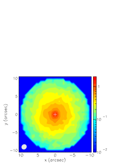
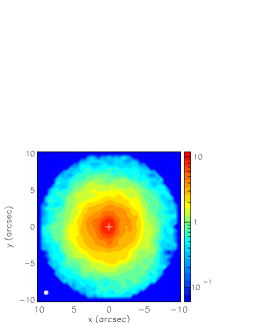
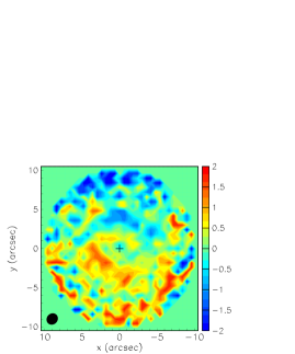
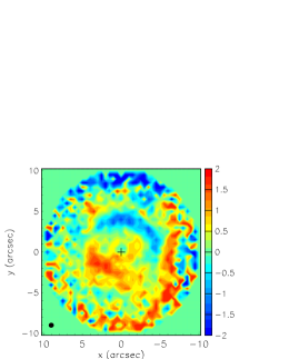
Figure 1: Sky maps of the integrated intensity (upper panels) and mean Doppler velocity (lower panels) for CO(1-0) (left) and CO(2-1) (right) emission. The intensity maps are integrated between $-$12 and 12 km s^-1 with respect to the stellar $V_{lsr}$. Units are Jy arcsec^-1km s^-1 and km s^-1. The beams are shown in the lower left corners.

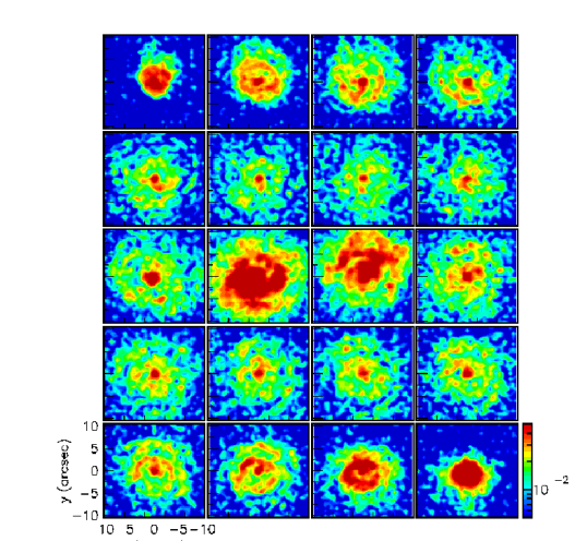
Figure 2: Channel maps of CO(1-0) emission grouped in bins of 1 km s^-1 between $-10$ km s^-1 and 10 km s^-1 with respect to the stellar $V_{lsr}$. The colour scale is in units of Jy arcsec^-2 km s^-1.

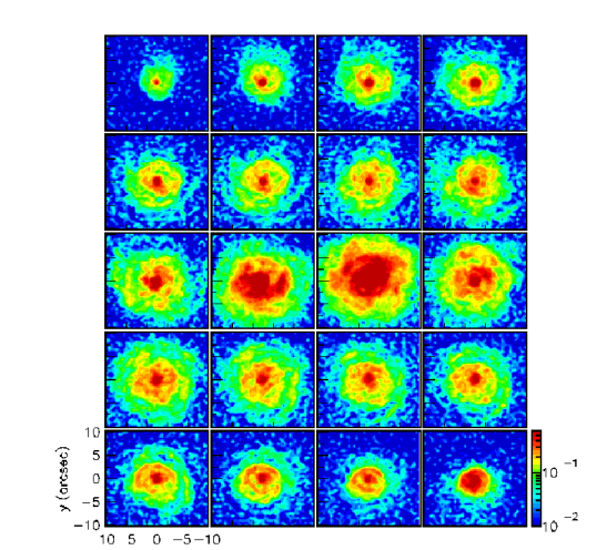
Figure 3: Channel maps of CO(2-1) emission grouped in bins of 1 km s^-1 between $-10$ km s^-1 and 10 km s^-1 with respect to the stellar $V_{lsr}$. The colour scale is in units of Jy arcsec^-2 km s^-1.

Table 1: Observing conditions.

	CO(1-0)	CO(2-1)
Beam FWHM	$0.78^{\prime\prime}\times 0.70^{\prime\prime}$	$0.33^{\prime\prime}\times 0.30^{\prime\prime}$
Beam PA	PA=$-56^{\circ}$	PA=$-80^{\circ}$
Max. baseline	1124 m	1400 m
Min. baseline	19 m	15 m
Time on source	98.3 min	52.4 min
Zero spacing	No	No
Noise (mJy beam-1/0.2 km s-1 bin)	7	6
Total flux, $R<13^{\prime\prime}$ (Jy km s-1)	110	549

The aim of the present article is limited to a presentation of the morphology and kinematics of the circumstellar envelope of EP Aqr inferred directly from the observational data without invoking a physical model. In addition to being a necessary preliminary to reliable physical modelling, it illustrates the type of constraints imposed on possible models. A discussion based on such a physical model, accounting in particular for the effect of temperature and absorption, is deferred to a forthcoming paper, together with the presentation and analysis of data obtained from other emission lines.

3 De-projection, effective emissivity and flux of matter

3.1 The method

We use Cartesian coordinates centred on the star with the $x$ axis pointing east, the $y$ axis pointing north and the $z$ axis parallel to the line of sight and pointing away from us. We also occasionally use polar coordinates in the plane of the sky, with radius $R=\sqrt{x^{2}+y^{2}}$ and position angle $\psi=\tan^{-1}(y/x)-90^{\circ}$ measured clockwise from north. We generally assume radial winds having axi-symmetric velocities about an axis making an angle $\varphi$ with the line of sight and projecting on the plane of the sky at position angle $\theta$. The projected axis is used as origin of stellar longitude $\omega$ and we call $\alpha$ the stellar latitude. The distance in space from the star is $r=\sqrt{R^{2}+z^{2}}$. Finally we call V the velocity vector and $V_{z}$ the Doppler velocity, projection of V on the $z$ axis.

Transformation relations from sky to stellar coordinates $(x^{\prime},y^{\prime},z^{\prime})$ read:

$$\begin{split}x^{\prime}&=x\cos\theta+y\sin\theta\\ y^{\prime}&=-x\sin\theta\cos\varphi+y\cos\theta\cos\varphi+z\sin\varphi\\ z^{\prime}&=x\sin\theta\sin\varphi-y\cos\theta\sin\varphi+z\cos\varphi\\ \end{split}$$ (1)

Observations provided by a radio telescope are in the form of data-cube elements, $f(x,y,V_{z})$ giving for each point $(x,y)$ on the plane of the sky (pixel) the distribution of the measured brightness as a function of Doppler velocity $V_{z}$. Before attempting to give a physical interpretation of what is observed, it is necessary to apply a de-projection to the observed image, namely to calculate, for each space point $(x,y,z)$ the effective emissivity $\rho$ and the three components of the velocity-vector (Diep et al. 2016). This is a largely under-determined problem and, in general, it cannot be solved. However, it becomes solvable once we know the velocity field $(V_{x},V_{y},V_{z})$ at each point in space. In that case, for each pixel $(x,y)$ the dependence on $z$ of the Doppler velocity is known and, to the extent that the corresponding relation can be inverted, it is possible to associate to each Doppler velocity $V_{z}$ a point $(x,y,z)$ in space. From the definition of the effective emissivity $\rho$, the intensity measured in this pixel reads

$$F(x,y)=\int{f(x,y,V_{z})dV_{z}}=\int{\rho(x,y,z)dz}$$ (2)

where the first integral spans the Doppler velocity range covered by the observation and the second integral extends over the whole line of sight, implying

$$\rho(x,y,z)=f(x,y,V_{z})\frac{dV_{z}}{dz}$$ (3)

The relation between $z$ and $V_{z}$ becomes particularly simple in the case of pure radial expansion, the velocity becoming a simple scalar $V$:

$$z/r=V_{z}/V$$ (4)

As $|z|$ needs not to exceed $r$, $V$ must be larger than $|V_{z}|$ for $z$ to be obtained from Relation (4). If not, part of the observed Doppler velocity spectrum is not accounted for by the calculated effective emissivity. But as long as this is the case, any scalar velocity field will produce an effective emissivity that reproduces perfectly the observations. Without further preconception about the nature of the space distribution of the effective emissivity, nothing else can be said. In the case of evolved stars, a natural hypothesis that might help with favouring specific solutions of the de-projection problem is the assumption of axi-symmetry (including spherical symmetry) of the effective emissivity, which is known to apply to the vast majority of such stars.

3.2 Orientation of the star axis

In order to measure the deviation from axi-symmetry of the effective emissivity $\rho(x,y,z)$, we define at each space point $(x,y,z)$ the quantity

$$D(R^{\prime},z^{\prime},\omega)=\frac{\rho(R^{\prime},z^{\prime},\omega)-<\rho(R^{\prime},z^{\prime})>}{\Delta\rho(R^{\prime},z^{\prime})}$$ (5)

where $R^{\prime}=\sqrt{x^{\prime 2}+y^{\prime 2}}$ and where $\Delta\rho(R^{\prime},z^{\prime})$ is the rms fluctuation of $\rho(R^{\prime},z^{\prime},\omega)$ about its mean over the volume of the data cube contributing to its evaluation (interpolation over 4 pixels and over the relevant range of the Doppler velocities). In case of perfect axi-symmetry, $D(R^{\prime},z^{\prime},\omega)$ cancels and we define $\chi^{2}_{axi}=<D^{2}(R^{\prime},z^{\prime},\omega)>$ as a figure of merit measuring the deviation from axi-symmetry. $\Delta\rho(R^{\prime},z^{\prime})$ accounts well for the dependence over the meridian plane of both experimental and systematic uncertainties. However, it overestimates them by a factor $\sim$3 and $\chi^{2}_{axi}$ is accordingly smaller than unity by a factor $\sim$10.

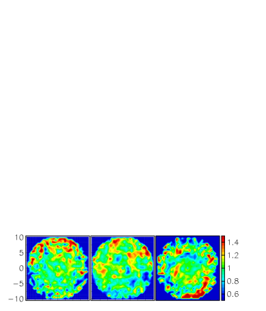
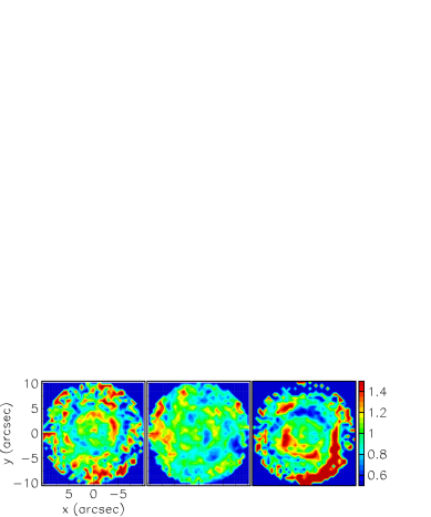
Figure 4: Sky maps of $\Delta(R,\psi)$ for $R<$10 arcsec for CO(1-0) (up) and CO(2-1) (down) emissions. Left panels are for $V_{z}<-2$ km s^-1, central panels for $|V_{z}|<$2 km s^-1 and right panels for $V_{z}>$2 km s^-1  as indicated in the Doppler velocity spectra displayed above the sky maps (This figure is reproduced from Figure 13, De-projection of radio observations of axisymmetric expanding circumstellar envelopes, Nhung et al., 2018, MNRAS, 408, 3324).

We have calculated the values taken by $\chi^{2}_{axi}$ for a very broad range of wind velocity configurations, from bipolar to equatorial, with or without radial velocity gradients, and we find that as long as $\varphi$ is kept small the de-projected effective emissivity is axi-symmetric. The reason is an intrinsic axi-symmetry of the data about an axis making a small angle with the line of sight for which we give evidence below. The channel maps of the measured brightness displayed in Figures 2 and 3, approximately rotation-invariant about the origin, already indicate the existence of such symmetry. But the study of the dependence of $\chi^{2}_{axi}$ on $\varphi$ and $\theta$ tells us in addition that the intrinsic symmetry is not spherical. In case of spherical symmetry, $\varphi$, and a fortiori $\theta$, are undefined, which is not the case for non-spherical axi-symmetry. To illustrate this important result in some detail, we show in Figure 4 a simplified version of Figures 2 and 3 aimed at illustrating the rotational invariance about the origin; the whole Doppler velocity range is split in only three intervals, the blue-shifted wing, the narrow central component and the red-shifted wing; moreover, rather than plotting the intensity, we plot the ratio $\Delta(R,\psi)=F(R,\psi)/<F(R,\psi)>_{R}$ where $<F(R,\psi)>_{R}$ is the mean value of $F(R,\psi)$ averaged over $\psi$ at fixed $R$. The rms values of $\Delta(R,\psi)-1$, which measure the violation of rotation invariance, are listed in Table 2; they are dominated by large distances from the star and never exceed 21% for CO(1-0) and 35% for CO(2-1) if one requires $R$ not to exceed 8 arcsec. There are obvious similarities between the maps of both emissions, giving confidence in the reality of the features that they may reveal.

Table 2: Rms deviation from unity (%) of $\Delta(R,\psi)$

	$R<10$ arcsec		$R<8$ arcsec
	CO(1-0)	CO(2-1)	CO(1-0)	CO(2-1)
$V_{z}<-2$ km s-1	30	56	20	35
$|V_{z}|<2$ km s-1	20	26	18	21
$V_{z}>2$ km s-1	32	70	21	35

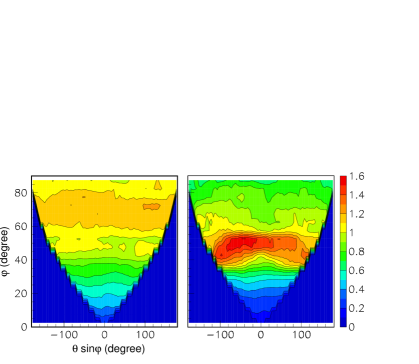
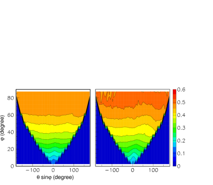
Figure 5: Dependence of $\chi^{2}_{axi}$ on $\theta\sin\varphi$ (abscissa) and $\varphi$ (ordinate) for a spherical wind $V_{0}$=12.5 km s^-1 (upper panels) or increasing from 0 to 12.5 km s^-1 between $r=0$ and $r=9$ arcsec (lower panels) and for CO(1-0) (left) and CO(2-1) (right) emissions. We use $\theta\sin\varphi$ rather than $\theta$ to have bins of constant solid angle coverage, $d\Omega=\sin\varphi d\theta d\varphi$.

As was remarked above, Figure 4 gives evidence for axi-symmetry about an axis close to the line of sight, but does not exclude spherical symmetry; on the contrary, it might seem more natural to see it as evidence for spherical symmetry: non-spherical axi-symmetry requires a symmetry axis nearly aligned with the line of sight, which one might feel is unlikely, even if such a feeling has no meaning (any pre-determined orientation is unlikely). However, the study of the dependence of $\chi^{2}_{axi}$ on $\varphi$ and $\theta$ invalidates such an interpretation. What $\chi^{2}_{axi}$ does is to measure the axi-symmetry of the de-projected effective emissivity about the axis of the axi-symmetric wind velocity field used for de-projection : the smaller $\chi^{2}_{axi}$, the better the axi-symmetry. As was mentioned above, in all cases that we have studied, we find that $\chi^{2}_{axi}$ is minimal at or near $\varphi=0$. In case of spherical symmetry, one would find instead that $\chi^{2}_{axi}$ is independent of $\varphi$.

To illustrate this point, we choose a spherical wind configuration to de-project the effective emissivity. In such a case, any axi-symmetry of the de-projected emissivity is an intrinsic property of the observations. When choosing an orientation ($\theta,\varphi$) of the wind axis used for de-projection, it is convenient to use bins of constant solid angle, $\varphi$ vs $\theta\sin\varphi$, accounting for the fact that when $\varphi=0$, $\theta$ is undefined. Figure 5 displays the result and gives evidence for a relatively steep minimum near $\varphi=0$ for both CO(1-0) and CO(2-1) emissions. The value of $\varphi$ for which $\chi^{2}_{axi}$ reaches twice its minimal value is 5^∘ for both emissions, giving the scale of the acceptable range of $\varphi$ values.

One might wonder if this conclusion may be influenced by the fact that we use wind configurations having velocities independent from the distance $r$ to the star. Figure 5 shows in the lower panels that such is not the case. The wind configuration used for de-projection is spherical but assumes a constant positive radial velocity gradient, the wind velocity increasing from 0 at $r=0$ to 12.5 km s^-1 at $r=9$ arcsec and staying there for larger values of $r$. The values of $\varphi$ for which $\chi^{2}_{axi}$ reaches twice its minimal value are now respectively 13^∘ and 15^∘ for CO(1-0) and CO(2-1) emissions. Indeed there exist arguments in favour of positive velocity gradients: the analysis of Nhung et al. (2015a) gives evidence for these and one might argue that the importance over the sky plane of the low velocity narrow central component of the Doppler velocity spectrum, rather than being due to an enhancement of the effective emissivity in the equatorial region, might rather be due to the presence of a spherical volume of gas in very slow expansion (this issue is addressed in some detail later in the text).

In the remainder of the article, we shall take $\varphi=0$, meaning that $\theta$ is irrelevant and that $(x^{\prime},y^{\prime},z^{\prime})=(x,y,z)$, $R^{\prime}=R$ and $\omega=\psi$. This choice is justified to the extent that the arguments that will be developed are not affected by small deviations, say below 20^∘, of the value taken by $\varphi$. It is not always the case; as we shall see in Section 3.5, polar latitudes prefer $\varphi=0$ but equatorial latitudes prefer $\varphi\sim 4^{\circ}$; more generally, independently from the adopted wind models, the narrow central Doppler velocity component shows evidence for axi-symmetry about an axis making an angle $\varphi$ with the line of sight of up to some 10^∘ to 15^∘ and projecting on the sky plane at a position angle of some 20^∘ to 30^∘ west of north.

3.3 Bipolar, spherical and equatorial winds

The following discussions use models of the wind velocity assuming radial expansion, independent of the distance $r$ to the star, of the form

$$V=V_{eq}+(V_{pole}-V_{eq})\sin^{2}\alpha$$ (6)

where $V_{pole}$ is the polar and $V_{eq}$ the equatorial velocity. For $V_{eq}=0$ we obtain a bipolar wind $V=V_{pole}\sin^{2}\alpha$, for $V_{pole}=V_{eq}$ a spherical wind and for $V_{pole}=0$ an equatorial wind $V=V_{eq}\cos^{2}\alpha$. In general $V_{pole}>V_{eq}$ produces bipolar winds, $V_{eq}>V_{pole}$ produces equatorial winds. In the spherical wind case, writing $V_{0}=V_{pole}=V_{eq}$ and $\lambda=V_{z}/V_{0}$, an effective emissivity of the form $\rho=\rho_{0}r^{-2}$ produces a Doppler velocity spectrum of the form $f_{sph}=\rho_{0}V_{0}^{-1}R^{-1}(1-\lambda^{2})^{-\frac{1}{2}}$ which displays no narrow central component and ends abruptly at $|V_{z}|=V_{0}$ below which values it is strongly enhanced. It takes an enhancement of the effective emissivity in the equatorial plane to produce a central velocity component. When the wind velocity departs from spherical, these general features are conserved. However, the difference between bipolar and equatorial winds is that the large values of $|V_{z}|$, being probed preferentially near the poles, require large values of $V_{pole}$, not of $V_{eq}$. This is illustrated in Figure 6, which displays the Doppler velocity spectrum accounted for by the de-projected effective emissivity for different values of the model parameters. Bipolar and spherical winds do not require $V_{pole}$ to exceed significantly 12.5 km s^-1 while equatorial winds are severely truncated as soon as $V_{pole}$ decreases below this value. For the whole Doppler velocity spectrum to be accounted for by an equatorial wind, we need to keep $V_{pole}$ sufficiently large: for a given shape of the wind velocity distribution, meaning a given $V_{eq}/V_{pole}$ ratio, we need to increase $V_{eq}$ accordingly. Examples are given in the next section. In other words, bipolar winds require smaller wind velocities than equatorial winds do.

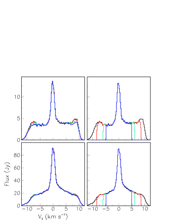
Figure 6: Doppler velocity spectra obtained from the de-projected effective emissivity for CO(1-0) (up) and CO(2-1) (down) emissions and bipolar (left) or equatorial (right) winds. In all cases the larger of $V_{pole}$ and $V_{eq}$ is set at 12.5 km s^-1 and the other takes values of 12.5 (black), 8.5 (red), 4.5 (green) and 0.5 (blue) km s^-1 respectively. The black histogram, corresponding to a spherical wind configuration, is undistinguishable from the measurement.

The end points of the measured Doppler velocity spectra, being much less abruptly cut-off than a $f_{sph}=\rho_{0}V_{0}^{-1}R^{-1}(1-\lambda^{2})^{-\frac{1}{2}}$ distribution, imply that the effective emissivity needs to be depressed near the poles. Moreover, the presence in the Doppler velocity spectra, everywhere on the sky plane, of a strong central narrow component requires an enhancement of the effective emissivity near the equator. This is clearly visible in Figure 7, which displays the de-projected effective emissivity obtained from a spherical wind having a radial velocity $V_{0}$=12.5 km s^-1.

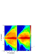
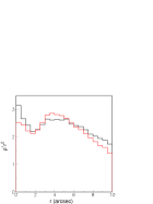
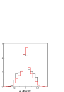
Figure 7: De-projected temperature-corrected effective emissivity $\rho^{*}$ (see Section 3.4) multiplied by $r^{2}$ obtained from a spherical radial wind of velocity 12.5 km s^-1. The half-meridian plane maps, from left to right CO(1-0) and CO(2-1) emissions, are shown in the left panels. The dependence on $r$ (middle) and on $\alpha$ (right) is shown for CO(1-0) (black) and CO(2-1) (red) in the right panels. The quantity $\rho^{*}r^{2}$ is in units that correspond approximately to a flux of matter of $\sim$10^-8 solar masses per steradian and per year for an expansion velocity of 10 km s^-1 or, equivalently, to a flux of matter of $\sim$0.5 10^-8 solar masses per steradian and per AU. A more precise evaluation, accounting for the effect of absorption, is deferred to a forthcoming paper (Hoai et al., in preparation).

The main features of the de-projected effective emissivity observed for a spherical wind, strong polar depression and equatorial enhancement, remain qualitatively present for other wind models for the same reasons as have been invoked in the spherical case. Also, the presence of a maximum at distances of some 3 to 6 arcsec from the star, will be seen in the next section to persist to some level over a broad range of models. However, introducing positive radial velocity gradients increases the contribution of a large and very slowly expanding gas volume to the narrow central component of the Doppler velocity spectrum, thereby lessening the need for an equatorial enhancement of the effective emissivity.

3.4 Dependence of the flux of matter on $r$ and $\alpha$

In the present section, we calculate the de-projected effective emissivity for different representative models of the wind velocity. From what was learnt in the preceding section, we always adjust the larger of $V_{pole}$ and $V_{eq}$ in such a way as to account for the whole observed Doppler velocity spectrum, but not larger than necessary. While sensible, this procedure cannot be rigorously justified. Moreover, we introduce a new parameter $n$ that allows for changing the angular width of the bipolar or equatorial outflow by writing

$$V =V_{eq}+(V_{pole}-V_{eq})(\sin^{2}\alpha)^{n}\,\mbox{for $V_{pole}>V_{eq}$ (bipolar)}$$

$$V =V_{pole}+(V_{eq}-V_{pole})(\cos^{2}\alpha)^{n}\,\mbox{for $V_{eq}>V_{pole}$ (equatorial)}$$

For $n$=1, as used in the preceding section, the half-width at half-maximum of the enhancement is 45^∘. It is 60^∘ for $n$=0.5 and 30^∘ for $n$=2.4. Our choice of parameters, meant to cover a very broad range of wind velocity configurations from strongly prolate (bipolar) to strongly oblate (equatorial), is listed in Table 3 together with the value of $V_{pole}$ or $V_{eq}$ adjusted to just account for the whole observed Doppler velocity spectra.

Table 3: Parameters of the representative wind models.

$n$ 0.5 1 2.4 Polar $V_{pole}$ 12 12 13.2 12 16.8 12.4 $V_{eq}/V_{pole}$ 1/4 3/4 1/4 3/4 1/4 3/4 $V_{eq}$ 3 9 3.3 9 4.2 9.3 Equatorial $V_{eq}$ 28.5 13.6 4.5 14.4 36 14.8 $V_{pole}/V_{eq}$ 1/3 3/4 1/3 3/4 1/3 3/4 $V_{pole}$ 9.5 10.2 11.5 10.8 12 11.1

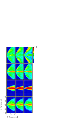
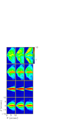
Figure 8: Left: dependence on latitude $\alpha$ (degrees in abscissa) of the wind radial velocity $V$ (km s^-1 in ordinate) for each of the twelve combinations $(V_{pole},V_{eq},n)$ of the model parameters as indicated in each sub-panel in the form of $n,V_{eq}/V_{pole}$. Right: Half-meridian-plane maps, averaged over longitude, of the de-projected effective emissivity corrected for temperature, $\rho^{*}$, multiplied by $r^{2}$ for each of the twelve combinations of the model parameters, ordered as in the left panel, and for CO(1-0) and CO(2-1) emissions separately (left to right). Units are as described in the caption of Figure 7.

Figure 8 (left) displays the corresponding dependence on latitude of the wind radial velocity $V$. In all cases (Figure 8 right), one obtains a very good agreement between CO(1-0) and CO(2-1) results after correction for temperature. More precisely, we define temperature-corrected emissivities $\rho^{*}=\rho/Q$ where, assuming Local Thermal Equilibrium (LTE), $Q=Q_{0}(2J+1)(2.8/T)\exp(-E_{up}/T)$; for CO(1-0) or respectively CO(2-1), $J$=1 or 2, the energy of the upper level of the transition $E_{up}$=5.5 K or 16.6 K and Einstein’s spontaneous emission probability $Q_{0}$=7.4 10^-8 s^-1 or 7.1 10^-7 s^-1. As radial dependence of the temperature we assume a form $T=32/r^{0.65}$ K with $r$ measured in arcsec (one of possible forms obtained in a preliminary radiative transfer calculation). This temperature correction is irrelevant to what follows, its only merit is to offer a direct and transparent comparison between the CO(1-0) and CO(2-1) results by making them commensurate. Figure 9 displays the dependence on $r$ of the flux of matter $\dot{M}$, approximated by the expression $\dot{M}=\rho^{*}Vr^{2}$, and on $\alpha$ of the temperature-corrected effective emissivity $\rho^{*}$ multiplied by $r^{2}$. Note that UV dissociation of the CO molecules causes a decrease of the density (Mamon et al. 1988) of the approximate form $f_{UV}={\frac{1}{2^{q}}}$ with $q=(\frac{r}{13})^{2.1}$ ($r$ in arcsec) obtained by assuming $\dot{M}=10^{-7}$ $\textup{M}_{\odot}$yr^-1 and $V\sim$7.5 km s^-1, meaning a factor $\sim$91% at $r$=5 arcsec and $\sim\frac{2}{3}$ at $r$=10 arcsec, close to what is observed.

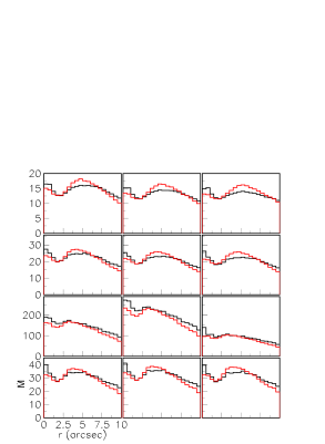
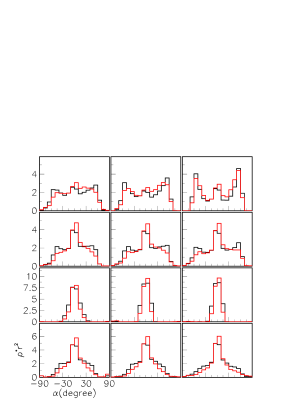
Figure 9: Dependence of the flux of matter on distance $r$ to the star (arcsec, left) and of the product $\rho^{*}r^{2}$ on latitude $\alpha$ (degrees, right) for each of the twelve combinations of model parameters, ordered as in Figure 8. Black is for CO(1-0) emission and red for CO(2-1) emission. Units are as described in the caption of Figure 7.

3.5 Deviations from axi-symmetry and disc rotation

The preceding section dealt with data averaged over longitude; we now study the dependence on longitude of the effective emissivity. For this study we make a particular choice of parameters meant to be typical of a likely configuration of velocities and densities: $(V_{pole},V_{eq},n)$=(12.5, 6, 1.5). Although we do not expect that the precise values of $\theta$ and $\varphi$ could matter much, we adjust them by minimising $\chi^{2}_{axi}$ in order to be as free as possible of deviations from axi-symmetry caused by a slight tilt of the star axis with respect to the line of sight. We perform the minimisation separately for the equatorial disc region, $|z^{\prime}|<$1 arcsec and the bi-conical outflow region, $|z^{\prime}|>$2 arcsec. The result is displayed in Figure 10. While the latter requires only $\varphi$ to be small, leaving $\theta$ essentially undefined, the former displays a clear minimum at $\varphi=3.8\pm 2.0^{\circ}$ where the error corresponds to a 10% increase in $\chi^{2}_{axi}$ with excellent agreement between the CO(1-0) and CO(2-1) lines. The value of $\theta$ at minimum is less well defined and of the order of 35 $\pm$ 35^∘. This is at strong variance with the behaviour of $\chi^{2}_{axi}$ in other regions of space and is commented on below. We therefore adopt these values of $\theta$ and $\varphi$ to map the effective emissivity, temperature-corrected and multiplied by $r^{2}$, in sixteen slabs of $z^{\prime}$ parallel to the equator, each 1 arcsec thick and covering between $z^{\prime}$=$-$8 arcsec and $+$8 arcsec. The CO(1-0) and CO(2-1) maps display strong similarity; in order to illustrate it, rather than showing them separately, we prefer to show in Figure 11 their half-sum and their half-difference. The former gives clear evidence for the bi-conical morphology of the polar outflow and for the presence of a flared disc, or of a ring, at the equator. The latter shows that the small difference between the emissions of the two lines decreases from being positive at large values of $|z^{\prime}|$ to negative at the equator, which probably reveals the imperfection of the radial dependence of the temperature adopted here. Deviations from axi-symmetry and from symmetry with respect to the equatorial plane are clearly significant but none of these suggests the presence of a specific feature worth mentioning; their main characteristic is their relatively modest amplitude.

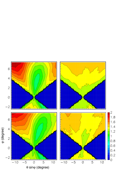
Figure 10: Dependence of $\chi^{2}_{axi}$ on $\theta\sin\varphi$ (abscissa) and $\varphi$ (ordinate) for CO(1-0) (up) and CO(2-1) (down) emissions and for $|z^{\prime}|<$ 1 arcsec (left) and $|z^{\prime}|>$2 arcsec (right). For convenience, $\chi^{2}_{axi}$ has been normalised to its minimal value and the colour code covers from minimum (1) to twice minimum (2) in each of the four panels.

The atypical behaviour of $\chi^{2}_{axi}$ in the disc region may suggest that it be related to rotation. Rotation of velocity $V_{rot}$ about an axis parallel to the line of sight implies $V_{z}$=0 while expansion of velocity $V_{exp}$ implies $V_{z}=V_{exp}\,z/r=V_{exp}\sin\alpha$. But, in the equatorial plane, a small tilt $\varphi$ of the star axis with respect to the line of sight generates Doppler components $V_{z}=V_{rot}\cos\omega\sin\varphi$ and $V_{z}=V_{exp}\sin\omega\sin\varphi$ : rotation and expansion cancel and reach their extrema at longitudes differing by 90^∘. Interpreting the effect of rotation as being caused by expansion produces identical values of the product $V\sin\varphi$ but position angles $\theta$ at 90^∘ from each other. However, when moving away from the equatorial plane, the Doppler component induced by rotation stays constant while that induced by expansion gets soon dominated by the $V_{exp}\sin\alpha$ term that takes opposite values in the blue-shifted and red-shifted regions. Moreover, in a plane of constant $z^{\prime}$ ($|z^{\prime}|<<r$) close to the equator, the Doppler component induced by expansion decreases like $\sim 1/R$ while that induced by rotation would decrease like $1/R^{\frac{1}{2}}$ in the Keplerian case.

These comments remind us of the difficulty to tell expansion from rotation (Diep et al. 2016); the study of $\chi^{2}_{axi}$ is equivalent to that of the behaviour of the narrow Doppler velocity component over the plane of the sky, as had been done in Nhung et al. (2015a); it is just more elegant in summarizing the available information in a single plot. However, a reliable interpretation in terms of competing expansion and rotation, as is observed, for example in the Red Rectangle (Tuan-Anh et al. 2015), would probably require data of better spatial resolution and signal-to-noise ratio and is beyond the scope of the present article. What has been made clear in the present analysis is that all the relevant information available on the precise orientation of the star axis is contained in the behaviour of the narrow central Doppler velocity component on the plane of the sky, meaning the kinematics of the equatorial disc or ring. Figure 10 is an elegant way to summarize its content but the interpretation is made difficult by the smallness of the tilt angle and a possible competition between rotation and expansion.

4 Discussion

By construction, any combination of model parameters chosen in the region explored in the preceding section produces an effective emissivity that gives a perfect description of the observations and that displays approximate axi-symmetry about the line of sight. Expressing a preference for a particular model implies therefore arguments of a different nature.

Qualitatively, the dependence on star latitude of the effective emissivity, and a fortiori of the flux of matter, is found to follow that of the wind velocity with the exception of the omni-present polar depression that has been discussed in Section 3.3. Indeed, if $V$ is small, $dV_{z}/dz$ is also small and so is $\rho$. As expected, the polar depression is slightly more important for CO(2-1) than for CO(1-0), reflecting the difference of behaviour of the corresponding velocity spectra near their end points. The presence of the polar depression had been overlooked in previous analyses. Another important result that had also been essentially overlooked in earlier analyses is that large equatorial expansion velocities produce a flared disc or ring of effective emissivity and mass loss. This becomes particularly spectacular in the case of equatorial winds, for which very high equatorial velocities may be required. In such cases, the bipolar outflow disappears completely, the mass loss occurring exclusively near the equator.

Remarkably, the radial dependence of the flux of matter is always found to display a maximum at distances between 3 and 6 arcsec, namely $\sim$ 500 AU, from the star. Note that a distance of 10 arcsec, meaning 1140 AU, is covered in only 540 years at a velocity of 10 km s^-1: we see but a very recent past of the history of the dying star.

Such maximum would imply that the assumption of stationary flow, implicit in the absence of radial dependence of the wind velocity, is not strictly obeyed: in that case, some episode of increased expansion must have occurred at some point in the recent history of the star, say in the past 1000 years or so. Violation of stationarity implies in turn the need to allow for a dependence of the wind velocity on the distance $r$ to the star. As mentioned earlier, this does not affect the presence of an intrinsic non-spherical axi-symmetry (Section 3.2) but lessens the contribution of the equatorial effective-emissivity to the central narrow component of the Doppler velocity spectrum (Section 3.3). However, the dominance of this narrow component in defining the orientation of the star axis (Section 3.5) pleads in favour of a slightly tilted equatorial enhancement: a slowly expanding spherical volume does not contribute any non-spherical axi-symmetry.

In any case, a significant violation of stationarity is not expected to affect the topology of the effective emissivity. We developed the argument previously in the case of Mira Ceti (Nhung et al. 2016, Diep et al. 2016) and it is even stronger in the present case where the morphology of the emission is considerably simpler, giving strong confidence in the reliability of the conclusions. Equatorial winds tend to give a steeper decrease of the flux of matter with distance than bipolar winds do, providing an additional argument in favour of bipolar winds. However, a detailed analysis in terms of temperature, optical depth and absorption is required before making this point more strongly.

In the same vein, we note small occasional differences between the radial dependence of the CO(1-0) and CO(2-1) flux of matter: these are unimportant and easily accounted for by small changes in the form adopted for the radial dependence of the temperature: they do not need to be further discussed in the present article.

Axi-symmetrical structures can be generated by different mechanisms (e.g., rotation, magnetic fields, binarity, …). For binary systems, Mastrodemos & Morris (1999) and Theuns & Jorissen (1993) predict the formation of spirals and arc-like structures. A visual inspection of the channel maps in Figures 2 and 3 reveals such sub-structures which therefore might hint to the presence of a binary system at the heart of EP Aqr.

The presence of an equatorial ring or flared disc raises the question of its possible rotation. This issue was addressed at the end of the preceding section and the very small tilt angle between the intrinsic axis of the observed brightness distribution and the line of sight precludes a reliable answer to this question.

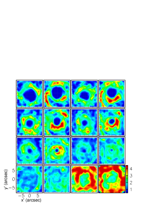
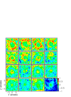
Figure 11: Maps of $\rho^{*}r^{2}$ in 1 arcsec wide $z^{\prime}$ intervals for the half-sum (left) and half-difference (right) of CO(1-0) and CO(2-1) emissions. Maps are shown in pairs associated with opposite values of $z^{\prime}$, negative for the leftmost, positive for the rightmost. From left to right and up to down, pairs are in the order of $z^{\prime}=\pm[8,7],\pm[7,6],\pm[6,5],...,\pm[2,1],\pm[1,0]$ arcsec. The wind parameters are $V_{pole}=12.5$ km s^-1, $V_{eq}=6$ km s^-1, $n=1.5$, $\varphi=3.8^{\circ}$ and $\theta=12^{\circ}$. Units are as described in the caption of Figure 7.

Finally, we recall that the irregularities of the emission that are revealed in Figure 11 are in large part significant to the extent that they appear in both CO(1-0) and CO(2-1) emissions but are of modest amplitude.

5 Summary and conclusions

In summary, a general analysis of recent high spatial resolution observations of the CO(1-0) and CO(2-1) emissions of the circumstellar envelope of EP Aqr has been presented. The data have been shown to display an intrinsic non-spherical axi-symmetry making a small angle with respect to the line of sight, constraining, in practice, the effective emissivity and the wind velocity distribution to obey similar axi-symmetry. Differences between the properties of CO(1-0) and CO(2-1) emissions have been shown to be consistent with the effect of a reasonable temperature gradient, the main point being an excellent agreement between the two. A detailed analysis of these observations in terms of density and temperature, rather than effective emissivity as in the present article, is the subject of another publication (Hoai et al., in preparation), which addresses issues that have been ignored here, in particular concerning effects of absorption and optical thickness. While such effects do not affect the qualitative conclusions of the present analysis, they do have significant quantitative consequences on the interpretation of the effective emissivity in terms of temperature and density. A preliminary radiative transfer calculation shows that absorption effects reach values between 10% and 40% on the effective emissivity over the meridian plane.

We have presented arguments that tend to prefer bipolar to equatorial winds, on the basis that the latter generally require higher wind velocities in order to account for the totality of the Doppler velocity spectra and produce a flux of matter decreasing faster with distance from the star. Such high wind velocities tend to increase the depression of emission in the polar regions, already important in any wind model because of the relatively smooth decrease of the observed Doppler velocity spectra near their end points. An enhancement of emission in the equatorial plane has been found necessary in order to produce the important narrow central component observed in the Doppler velocity spectra everywhere on the sky plane.

Significant irregularities of the emission (significant in that they are seen consistently in both CO(1-0) and CO(2-1) emissions) have been observed, however at a level not exceeding typically 40% and insufficient to provide clear evidence for important specific features.

Evidence for a clear influence of the orientation of the star axis on the behaviour of the narrow Doppler velocity component in the sky plane has been provided using as figure of merit a quantity, $\chi^{2}_{axi}$, that summarises elegantly the available information. However, the possible competition of rotation and expansion in the equatorial disc or ring makes the interpretation difficult and beyond the scope of the present article.