Probing Cosmic Strings with Gravitational-Wave Fringe

Abstract

Cosmic strings are important remnants of early-Universe phase transitions. We show that they can be probed by Gravitational Waves (GWs) from compact binary mergers. If such chirping GW passes by a cosmic string, it is gravitationally lensed and left with a characteristic signal of the lensing – the GW fringe. It is observable naturally through the frequency chirping of GWs. This allows to probe cosmic strings with small tension $\Delta=8\pi G\mu=10^{-6}\text{ -- }10^{-10}$, just below the current constraint, at high-frequency LIGO-band and mid-band detectors. Although its detection rates are estimated to be small, even a single detection can be used to identify a cosmic string. Contrary to the stochastic GW produced from loop decays only in local $U(1)$ models, the GW fringe can directly probe straight strings model independently. This is also complementary to the existing probes with the strong lensing of light.

1 Introduction

It is believed that the early Universe has evolved down to the Standard Model of particle physics from a more unified or fundamental theory by experiencing several phase transitions. The spontaneous symmetry breaking of a (global or gauge) $U(1)$ symmetry must have produced cosmic strings Kibble:1980mv . Cosmic strings are one-dimensional topological field configurations, produced also from string theory and vortex-like solutions of quantum field theory. Once produced, they gradually evolve into the scaling regime, where the total energy density of strings and closed string loops remains constant with the expansion of the Universe Vanchurin:2005pa ; Rocha:2007ni ; Kibble:1976 ; Vilenkin:1984ib . Thus, observing cosmic strings that remain today can give important clues on the physics of the early Universe.

Cosmic strings are characterized by its tension $\mu$ (energy density per unit length), given by $G\mu=v^{2}/m_{\rm Pl}^{2}$ with the symmetry-breaking vacuum expectation value $v$ of a $U(1)$ symmetry. The thickness of a gauge string is small of order $1/v$ so that it is a highly localized one-dimensional energy clump. The global string has its energy more spread in space stored in the Goldstone fields wrapping around the string, but their gravitational effects on null rays (photons and GWs as in this paper) are almost equivalent up to a marginal logarithm factor that describes the spatial spread Harari:1988wa . As string’s high local energy density disturbs the homogeneity of the CMB power spectrum, the tension is constrained to be $G\mu\lesssim 10^{-7}$ (or $\Delta\equiv 8\pi G\mu\lesssim 10^{-6}$ in our notation) Charnock:2016nzm . Although cosmic strings consequently cannot be the dominant fraction of dark matter (DM) or the seed of structure formation, their high local energy density may still leave important observable signatures.

Cosmic strings have been probed mainly by CMB anisotropies, stochastic GWs radiated from gauge string loops, and by their gravitational lensing on lights. The GW radiation from string loops is an essential energy-loss mechanism in the evolution of a string network into the scaling regime, where the string network’s energy density can remain safely small Vanchurin:2005pa ; Rocha:2007ni ; Kibble:1976 ; Vilenkin:1984ib . Thus, the stochastic GW is a prime observable of cosmic strings that is actively searched for Kuroyanagi:2012jf ; Blanco-Pillado:2017rnf ; Ringeval:2017eww ; Abbott:2017mem (this may lead to a constraint as strong as $G\mu\lesssim 10^{-11}$, albeit model dependencies), and its spectrum can also probe the cosmological evolution history of the Universe Cui:2017ufi ; Cui:2018rwi . On the other hand, global strings evolve into the scaling regime through the rapid decay of loops by radiating off Goldstone bosons, so the stochastic GW signal is absent. Instead, what always remains model independently is the order-one number of long (at least Hubble-sized) strings per horizon Consiglio:2011qe ; Harari:1987ht ; Sikivie:1990sb , as the causality requires. The long string can be directly probed by the strong lensing of light (multiple images resolved in angle or arrival time) Vilenkin:1981zs ; Gott:1984ef and femto-lensing of gamma-ray bursts (GRBs) Yoo:2012dn ; Suyama:2005ez , but the detection rates are small as will be discussed. Therefore, new independent probes are needed to boost the detection prospects.

In this paper, we study the chirping GW from binary mergers as a probe of cosmic strings. The new observable is the interference fringe of GWs produced by the gravitational lensing of cosmic strings; this is similar to the GW fringe produced by compact dark matter such as primordial black holes Jung:2017flg ; Nakamura:1997sw . The fringe is naturally observed through the chirping (particular pattern of time-dependent frequency evolution) of GWs. Thus, the sensitivity range of $\Delta$ depends on both the frequency band and frequency resolution of measurements. We will show that the LIGO frequency band ($5\text{ -- }5000$ Hz) and the mid-frequency band ($0.1\text{ -- }10$ Hz) are particularly useful, as they can probe $\Delta\lesssim 10^{-6}$ just below the current constraint.

We start by calculating the lensing fringe and its detection rate in Sec. 2 and Sec. 3, respectively. Then we present numerical results and analyze detection prospects in Sec. 4, discuss further phenomenology in Sec. 5, and conclude at the end.

2 Lensing fringe from cosmic strings

2.1 Straight strings

The space-time geometry around a straight (gauge) string is described by a conical space Vilenkin:1981zs

$$ds^{2}\,=\,dt^{2}\,-\,dZ^{2}\,-\,dR^{2}\,-\,\left(1-\frac{\Delta}{2\pi}\right)^{2}R^{2}d\hat{\phi}^{2},$$ (1)

where the string is placed along the $Z$-axis and $\hat{\phi}$ is measured around the string. By the redefinition of the azimuthal angle $\phi=(1-\Delta/2\pi)\hat{\phi}$, the conical space can be viewed as the Euclidean flat space with a deficit angle $\Delta\equiv 8\pi G\mu$. The deficit angle is defined by a boundary condition on the GW amplitude $h(\phi=0)=h(\phi=2\pi-\Delta)$ in the plane perpendicular to the string, with the allowed range $0\leq\phi\leq 2\pi-\Delta$. The gravitational effect of global strings on null rays is described by a similar deficit angle Harari:1988wa ; thus, we simply use the same metric and lensing calculation for both cases.

There is a freedom to choose the direction of $\phi=0$ in mapping the conical space to the Euclidean space with deficit angle. In the presence of a GW source, it is particularly convenient to choose such that $\phi=0$ is mapped to point to the source in the conical space. In the Euclidean space, this is equivalent to the source located at $\phi=0$ and $\phi=2\pi-\Delta$ simultaneously, which guarantees the boundary condition to be satisfied. Now, within the allowed range of $\phi$, null rays from the source are propagated according to the usual Helmholtz equation on the Euclidean space. Consequently, the GW rays arriving at the observer can be obtained by the Kirchhoff diffraction integral of freely propagating rays around the string schneider:1992 .

The gravitationally lensed GW waveform (that an observer measures) is parameterized in the frequency domain as

$$\widetilde{h}^{L}(f)\,=\,\widetilde{h}(f)\,F(f)\,e^{if\phi_{m}}.$$ (2)

Here, $\widetilde{h}(f)$ is the unlensed waveform which is explained in Sec. 3.2. The complex lensing amplification $F(f)$ is the solution of the diffraction integral Yoo:2012dn

$$F(f) = e^{-i\frac{fw}{2}(1+2y)}\left\{1-\frac{1}{2}\text{erfc}\left[\sqrt{\frac{fw}{2i}}(1+y)\right]\right\}$$ (3)

$$\,+\,e^{-i\frac{fw}{2}(1-2y)}\left\{1-\frac{1}{2}\text{erfc}\left[\sqrt{\frac{fw}{2i}}(1-y)\right]\right\},$$

where

$$w\,\equiv\,2\pi\frac{d_{L}d_{LS}}{d_{S}}\left(\frac{\Delta}{2}\right)^{2}\,\simeq\,1.6\,{\rm sec}\,\times\left(\frac{d_{L}}{100\ \text{Mpc}}\right)\left(\frac{d_{LS}}{100\ \text{Mpc}}\right)\left(\frac{100\ \text{Mpc}}{d_{S}}\right)\left(\frac{\Delta}{10^{-8}}\right)^{2}$$ (4)

is the characteristic path difference among the GW rays. $y\equiv 2\phi_{S}/\Delta$, where $\phi_{S}$ is the azimuthal angle $\phi$ between the two lines, one connecting the observer and the string and the other connecting the string and the source, on the plane perpendicular to the string. As physics is symmetric with respect to $y\rightarrow-y$, hereafter we deal with only $y>0$. We denote the angular diameter distance by $d$, luminosity distance by $D$, and comoving distance by $\chi$; the subscripts $L,S$ and $LS$ denote the distances to the lens, source and between the lens and source, respectively. Since distances and $\Delta$ are combined into one variable $w$ on which lensing amplification $F(f)$ depends, they cannot be measured separately from the observed waveform alone. Lastly, the extra phase in Eq. (2)

$$\phi_{m}\,=\,\frac{w}{2}+wy$$ (5)

makes the arrival time of the fastest path to zero so that we can focus only on the relative phases among the rays; this shall be consistent with our choice of $t_{c}=0$ in the GW waveform as discussed in Sec. 3.2.

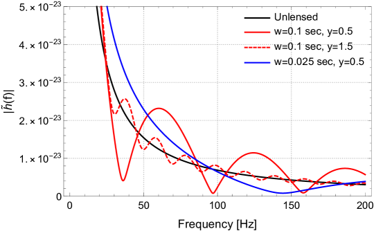
Figure 1: GW fringes from cosmic-string lensing in the frequency domain. The benchmark GW is from 30$M_{\odot}$-30$M_{\odot}$ binary at 400 Mpc of luminosity distance: unlensed (black), lensed by a cosmic string with $w=0.1$ sec and $y=0.5$ (red-solid), $w=0.1$ sec and $y=1.5$ (red-dashed), $w=0.025$ sec and $y=0.5$ (blue). The $w$ and $y$ are the characteristic path difference and angular impact parameter, respectively, defined in Eq. (4) and below.

In Fig. 1, we show an example unlensed waveform $|\widetilde{h}(f)|$ and its lensed waveforms $|\widetilde{h}^{L}(f)|$ in various lensing environments. The lensed waveforms oscillate with respect to the unlensed waveform, having local maxima at regular frequency intervals. The oscillation is due to alternating constructive and destructive interferences between the rays contributing to the $F(f)$. We name this interference fringe as the “GW fringe” Suyama:2005ez ; Nakamura:1999ptps ; Jung:2017flg . It has characteristic features that not only allow efficient detection but also distinction from other chirping effects and other kinds of lenses.

Fig. 1 shows those characteristic features of GW fringes from cosmic strings, in their oscillation amplitudes and widths in the frequency domain, with three example cases. For $y<1$, the interference occurs maximally so that $|F|$ oscillates from nearly 0 to nearly 2 in the whole range of $f$, for any values of $w$ (red and blue solid lines with $y=0.5$ in Fig. 1). On the other hand, for $y>1$, the amplitude of the interference becomes smaller for larger $f$, $w$, and $y$. The amplitude decreasing with $f$ shown in the red-dashed ($y=1.5$) is a character of the diffraction.

These can be analytically understood in the limit $fw\gg 1$ (or, more precisely, $fw(1\pm y)^{2}\gg 1$), in which the phase shifts among the rays ($\sim fw$) span many numbers of the fringe period. In this limit, the amplification factor becomes the interference among three rays:

$$F(f)\,\simeq\,e^{-i\frac{fw}{2}(1+2y)}\,+\,\frac{1+\text{sgn}(1-y)}{2}e^{-i\frac{fw}{2}(1-2y)}\,-\,\frac{2}{\sqrt{2\pi fw}(1-y^{2})}e^{i(\frac{fw}{2}y^{2}+\frac{\pi}{4})}.$$ (6)

The first two terms are identified as the result in the geometrical optics limit and the last term is a diffracted ray. For $y<1$, the two geometrical-optics terms are deflected rays in each side of the string; equivalently, in the Euclidean space with a deficit angle, the two rays arrive at us straightly from the two images of the source at $\phi=0$ and $\phi=2\pi-\Delta$. They correspond to the usual two rays in the geometrical optics limit of the point-mass lensing, but one of them (the second term) has its amplitude decreased by half for $y=1$ and disappears for $y>1$.

The third term in Eq. (6) is the ray diffracted from the cosmic string. The diffraction nature is encoded in both the amplitude and the phase. The phase (or path difference) implies that this ray first hits the string and then propagates to the observer (actually spreads out all directions). The amplitude decreasing with $f$, $\propto 1/\sqrt{fw}(1-y^{2})$, is indeed a common feature of diffraction of any waves; it is remarked that this term is exactly derived by the geometric theory of diffraction Keller:1962josa . Such $f$ dependence of the amplitude for $y>1$ is shown in Fig. 1.

After all, all three rays interfere. For $y<1$, all three rays reach the observer, and the two geometric rays make full interference while the effect of a diffracted ray is relatively suppressed. For $y>1$, although the diffracted ray weakens with increasing $y$, this produces the GW fringe. So in this case, the amplitude of a fringe is proportional to the amplitude of a diffracted ray, $1/\sqrt{fw}(1-y^{2})$.

Another more important feature in Fig. 1 is that all three cases have constant fringe widths in the frequency domain. The width $f_{\rm width}$ is determined by phase shifts among the major interfering rays – two geometric rays for $y\leq 1$ and one geometric ray and the diffracted ray for $y>1$ – such that $f_{\rm width}$ times the path difference equals to unity. By reading the phases in Eq. (6), we obtain

$$f_{\rm width}\,\simeq\,\begin{cases}\pi/wy,&\text{for }y\leq 1\\ 4\pi/w(1+y)^{2},&\text{for }y>1\end{cases}.$$ (7)

For example, the width $f_{\rm width}\simeq 4$ Hz for $\Delta=10^{-8}$, $d_{L}=d_{LS}=100$ Mpc, $d_{S}=200$ Mpc, and $y=1$ (giving $w\simeq 0.8$ sec). The width is indeed constant in $f$ for the given lensing situation, so that fringes repeat with a constant period in the frequency domain as discussed and shown in Fig. 1. This is a general feature of lensing fringes Jung:2017flg as the characteristic time-delay is determined by the geometry. But cosmic-string fringes also have features distinct from point-mass fringes as will be discussed in Sec. 5.1. The constant width is also a key property that allows efficient discrimination against various oscillating effects of chirping as will be discussed in Sec. 3.2.

2.2 Loops

The gauge string is accompanied by loops, which can also give rise to lensing effects. In this subsection, we first calculate the total length of the loops and then show that its large fraction can be treated as straight strings in the lensing perspective.

The string-loop network in the scaling regime is assumed to be the one-scale model Caldwell:1991jj with the matter-dominated universe. In this model, loops have initial length $L(t_{B})=\alpha l(t_{B})$ at their birth time $t_{B}$, where $l(t)$ is the particle horizon at time $t$ and $\alpha$ is a free parameter with a wide range $\alpha=0.1$ – $10^{-5}$ Caldwell:1991jj (we choose a specific value for numerical results at the end of this section). Once a loop is formed, it radiates GW and shrinks with the energy-loss rate $dE/dt=-\Gamma G\mu^{2}$, where $\Gamma\approx 50$ is a constant determined by numerical simulation Caldwell:1991jj . Then the distribution of length-weighted comoving number density at some given time $t$ is Mack:2007ae

$$L\frac{dn(t)}{dL}\,\approx\,C^{\prime}H_{0}^{2}\frac{L}{\left(L+\frac{1}{3}\Gamma G\mu l(t)\right)^{2}},$$ (8)

where $n(t)$ is the total comoving number density of the loops, $H_{0}$ is the Hubble parameter today, and $C^{\prime}$ is a constant to be determined by numerical simulations. In this derivation, $l(t)=3t$ for the matter dominated universe and $\alpha\gg\Gamma G\mu$ are used. The time dependence kept until this step finally drops out in the energy density fraction $\Omega_{\rm loop}$, as should be in the scaling regime

$$\Omega_{\rm loop}\,\approx\,\frac{8\pi}{3}G\mu C^{\prime}\left[\ln\left(\frac{3\alpha}{\Gamma G\mu}\right)-1\right].$$ (9)

Meanwhile, the number of straight strings (at least as long as the Hubble length) in a Hubble volume was also calculated by simulations Caldwell:1991jj ; Consiglio:2011qe , yielding ${\cal O}(1)$ albeit some uncertainties; similarly, the number of global strings is also estimated to be ${\cal O}(1)$ per Hubble volume Harari:1987ht ; Sikivie:1990sb . In this work, we simply take the string number density to be one in a Hubble volume, so that $\Omega_{\rm cs}=8\pi G\mu/3$ (subscript cs refers only to the straight strings). Therefore, the energy ratio of total loops to total straight strings is

$$\frac{\Omega_{\rm loop}}{\Omega_{\rm cs}}\,=\,C^{\prime}\left[\ln\left(\frac{3\alpha}{\Gamma G\mu}\right)-1\right].$$ (10)

This is rather a generic result of the one-scale model. We use $\Gamma=50$ and $C^{\prime}=0.625$, where the latter choice is the one that we found to fit the recent simulation result Blanco-Pillado:2013qja . The ratio is minimal $\Omega_{\rm loop}/\Omega_{\rm cs}\approx 1.1$ for $\Delta=10^{-6}$ and $\alpha=10^{-5}$ and grows to $\approx 12.6$ for $\Delta=10^{-10}$ and $\alpha=0.1$. Thus, for the most part of the parameter space, a large fraction of string network’s energy reside in the loop.

What kind of lensing effects do loops produce? Although a loop at a far distance produces the Schwarzschild metric of the total loop mass, it can be treated as a straight string in its vicinity. Roughly speaking, the loop produces the same lensing effects as straight strings when the loop segment produces a pair of double images of a source just behind it. A loop at angular-diameter distance $d$ and oriented to face the observer can be regarded as a straight string if the loop radius is greater than $d\Delta/2$ Vilenkin:1984ea . In terms of loop length $L$ and comoving distance $\chi$, this means

$$L\,>\,8\pi^{2}G\mu\,a(t(\chi))\,\chi,\qquad\textrm{(minimum loop for simple lensing)}$$ (11)

where $a(t)$ is the scale factor at time $t$. This is valid in the vicinity of a loop, and here is where detectable lensing fringes are produced.

Therefore, the total fraction $\xi_{l}$ of the loop length that can be treated as a straight string (for a given $\chi$) is approximately the length distribution Eq. (8) integrated over the range that satisfies Eq. (11) as

$$\xi_{l}(\alpha,\Delta,\chi)\ \approx\ \frac{\int^{\alpha l(t)}_{8\pi^{2}G\mu a(t)\chi}\,L/[L+\frac{1}{3}\Gamma G\mu l(t)]^{2}\,dL}{\int^{\alpha l(t)}_{0}\,L/[L+\frac{1}{3}\Gamma G\mu l(t)]^{2}\,dL}.$$ (12)

Here, the upper bound comes from the longest loops at time $t(\chi)$. For the typical distance of 1 Gpc, the fraction is minimal $\xi_{l}\approx 0.97$ for $\alpha=10^{-5}$ and $\Delta=10^{-6}$ and grows toward $\xi_{l}=1$ for larger $\alpha$ and smaller $\Delta$. Thus, most of the total loop-length can be treated as a straight string.

In all, in our final results, we assume $\xi_{l}=1$ and use the energy fraction $\Omega_{\rm loop}/\Omega_{\rm cs}$ in Eq. (10) with $\alpha=0.1$ Abbott:2017mem .

3 Lensing detection estimation

3.1 Detection criteria

In this paper, we estimate the number of GW events with detectable lensing fringe in a simplified way. We measure the likelihood of the existence of fringes by a simple least chi-square test between the lensed and (best-fit) unlensed waveforms. It is based on the assumption that the un-fit differences can be well associated with the fringe because lensing fringes are characteristically different from other features of chirping GWs, as will be discussed in Sec. 3.2. This is our main assumption and simplification.

First of all, the chirping GW itself must be detected confidently with large signal-to-noise ratio (SNR)

$$\textrm{SNR}\,\geq\,10.$$ (13)

Although lensed GWs will not be perfectly matched by unlensed waveforms in the discovery stage with matched filtering method, the overall waveform is still dominated by the chirping itself while lensing effects are subdominant perturbations. Thus, we assume that the discovery of lensed GWs using unlensed waveforms can still be well done. For simplicity, we use unlensed SNR.

Second, for confidently detected GWs, the log-likelihood $-\ln{\cal L}$ of the existence of lensing fringes is simply measured by the least chi-square method (see Appendix A and Jung:2017flg ; Dai:2018enj ) and required to be

$$-2\ln{\cal L}\,\equiv\,4\int^{f_{\rm max}}_{f_{\rm min}}\frac{|\widetilde{h}^{L}(f)-\widetilde{h}_{\rm best-fit}(f)|^{2}}{S_{n}(f)}\ df\,>\,9.$$ (14)

The $\widetilde{h}_{\rm best-fit}(f)$ is the unlensed GW waveform which minimizes the likelihood (see Sec. 3.2 for unlensed waveforms and fitting parameters that we use), and $\widetilde{h}^{L}$ is the lensed waveform in Eq. (2); $S_{n}(f)$ is the power spectrum of the noise and $f_{\rm min,max}$ are the frequency range of the measurement. The large value of the $-\ln{\cal L}$ means that there are notable features in the GW that cannot be fit well by unlensed waveforms. Such features are assumed to be well associated with the fringe. Thus, $-\ln{\cal L}$ is equivalent to the likelihood of the fringe.

Lastly, the fringe oscillation must be well resolved in the frequency domain

$$f_{\rm width}\,\geq\,2f_{\rm resol}.$$ (15)

Otherwise, oscillations will be averaged out in measurements. Here, $f_{\rm width}$ is the width given by Eq. (7), and $f_{\rm resol}$ is the frequency resolution of the measurement estimated by the discrete Fourier transform, hence given by the inverse of the total duration $T$ of a chirping measurement as

$$f_{\rm resol}(f_{\rm max},f_{\rm min},{\cal M}_{z})\,=\,\frac{1}{T(f_{\rm max},f_{\rm min},{\cal M}_{z})}\,\simeq\,1.5\,{\rm Hz}\,\times\left(\frac{{\cal M}_{z}}{100\,M_{\odot}}\right)^{5/3}\left(\frac{f_{\rm min}}{10\,\text{Hz}}\right)^{8/3},$$ (16)

where $f_{\rm min}\ll f_{\rm max}$ is used in the last approximation and ${\cal M}_{z}$ is the redshifted chirp mass. The factor 2 in Eq. (15) is a conservative factor that may account for additional uncertainties; we will later briefly discuss how our results change with this factor.

With these simplified criteria in Eq. (13) – (15), the detection rate is calculated by integrating over all possible source and string properties (locations, masses, and etc) for detectable lensing. See Appendix B for more details. The rate is a function of comoving merger-rate density, comoving cosmic string density $n_{cs}$, and detector specs $\equiv\{f_{\rm max},f_{\rm min},S_{n}(f)\}$. As for the merger-rate density, we assume all binary mergers are composed of two identical black holes (BHs) with the total mass $M$ (hereafter masses are always redshifted ones). Such comoving merger-rate density was calculated in Belczynski:2016obo with the latest version in http://www.syntheticuniverse.org/stvsgwo.html ; we take the M10 optimistic prediction at $z_{S}=0.1$, denoted as $n_{s}(M)$. $n_{s}(M)$ is given for several selected mass bins. The comoving cosmic string density is chosen to be 1 in a Hubble volume, $n_{cs}=(4.3\times 10^{3}\ \text{Mpc})^{-3}$, by referring to the scaling solution Caldwell:1991jj ; Consiglio:2011qe ; Harari:1987ht ; Sikivie:1990sb ; if the string number density is greater than 1 in a Hubble volume, the detection rate will increase proportional to the number density. For simplicity, those densities are assumed to be isotropic and constant in redshift (although $n_{s}(M)$ at high redshift may be larger Belczynski:2016obo ).

3.2 Leading-order waveforms

Following Jung:2017flg , we use the leading-order quadrupole chirping waveform in the inspiral stage. The observed waveform can be written in the form

$$\widetilde{h}(f;A_{0},\phi_{0})\,=\,A_{0}f^{-7/6}e^{i\Psi(f,t_{c}=0)\,+\,i\phi_{0}},$$ (17)

for the purpose of calculating the likelihood in Eq. (14). The frequency dependences of the chirping are explicitly shown in the amplitude and the phase

$$\Psi(f)\,=\,2\pi ft_{c}\,+\,\frac{3}{128}(\pi{\cal M}_{z}f)^{-5/3},$$ (18)

where $t_{c}=0$ (coalescence time) as discussed in regard of Eq. (5). In the leading-order inspiral waveform, there are no other frequency-dependent features (see below for ignored effects). Thus, it is a good approximation to estimate the fringe detectability by minimizing $-\ln{\cal L}$ over two fitting parameters – the overall amplitude $A_{0}$ and the overall phase shift $\phi_{0}$ Jung:2017flg ; Dai:2018enj . The inspiral-stage measurements are integrated up to the innermost stable circular orbit $f_{\rm max}=f_{\rm ISCO}=(3\sqrt{3}\pi M)^{-1}$ with the total binary mass $M$.

However, the waveform in Eq. (17) ignores several effects that can produce oscillations in the waveform. First, the time-variations of detector orientations are ignored, either because they are almost constant during short measurement time or their time variations (daily or hourly) are very different from fringe oscillations. Second, the BH spin precession and orbital eccentricity are not considered. The former generally becomes quicker with inspiral (hence growing with frequency), and the latter quickly becomes small as the orbit circularizes during the chirping. Thus in general, they cannot mimic lensing fringes which have constant frequency widths and particular amplitudes. Last, the waveform dismisses the merger and ringdown phases as well as higher-order post-Newtonian effects. These become most relevant for relatively heavy binaries with total mass $M\gtrsim 50M_{\odot}$ Ajith:2008 ; Khan:2016 , while the majority of binary populations that we consider is lighter Belczynski:2016obo . Thus, it is a good approximation to use leading-order waveforms with the least chi-square test for estimating the prospects of GW fringe detection.

This simplified analysis was already used in Ref. Jung:2017flg for the point-mass lensing, and was found to be in reasonable agreement with more dedicated later works that even included BH spin effects Christian:2018vsi ; Dai:2018enj ; Lai:2018rto . Such good agreement stems again from the characteristic behaviors of fringes – constant widths and particular amplitudes. Thus, we assume that the same simplifications can work well for the cosmic-string lensing too, while encouraging more dedicated analyses.

4 Prospects at future detectors

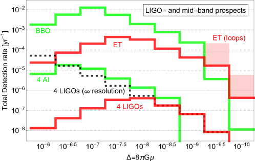
Figure 2: Expected detection rates of the GW fringe from cosmic strings at aLIGO, ET, AI, and BBO. The former two are high-frequency LIGO-band detectors (red), while the latter two are mid-band detectors (green). Last one-hour measurements in the mid-band detectors are used, while full measurements are used for the high-frequency detections. 4 detectors for aLIGO and AI are added, while 1 detector for ET and BBO. The black dashed is the aLIGO result with infinite frequency resolution. The red shaded region indicates additional loop contribution (if they exist) for ET. The cosmic string number abundance is 1 per horizon, and the GW merger rate is from Belczynski:2016obo ; http://www.syntheticuniverse.org/stvsgwo.html . The results are based on simplified analysis in Sec. 3.

The estimated detection rates are shown in Fig. 2. Shown benchmark detectors are high-frequency LIGO-band detectors (probing roughly 5 or 10 – 5000 Hz) and mid-band detectors (roughly 0.1 – 10 Hz). The former is represented by four advanced LIGO(aLIGO) detectors with design sensitivity TheLIGOScientific:2016agk (lower red) and one Einstein Telescope(ET) detector Hild:2010id (upper red), but ET has $10-50$ times smaller noise; the latter is by four Atom Interferometer(AI) detectors Graham:2016plp ; Graham:2017pmn (lower green) and one Big Bang Observatory(BBO) detector Yagi:2011wg (upper green), but BBO has 10 – 50 times smaller noise. Only last one-hour measurements of each GW in the mid-band are used (usually starting around 1 Hz) although GWs typically spend longer time in the mid-band, while full LIGO-band measurements (much shorter than an hour) are used. Only straight strings are included, but additional loop contributions that exist in local $U(1)$ models are shown for ET results (red shaded).

Above all, the overall detection rates of straight-string lensing fringes are much smaller than 1 per year. Thus, it is difficult to put constraints on the cosmic strings with just chirping GW observations. 4 aLIGOs are expected to detect $\sim 10^{-7}\,\text{yr}^{-1}$, 4 AIs $\sim 10^{-6}\,\text{yr}^{-1}$, ET $\sim 10^{-4}\,\text{yr}^{-1}$, and BBO $\sim 10^{-3}\,\text{yr}^{-1}$. The overall detection rates can be understood as follow. Since the majority of detectable lensing occurs for $|y|\lesssim\mathcal{O}(1)$, the lensing-detectable volume is $V\sim\Delta\cdot\chi_{\rm max}^{3}$ (where $\chi_{\rm max}$ is the comoving horizon distance of a detector; see Appendix B for details), and consequently

$$\text{detection rate}\,\sim\,(\Delta\cdot\chi_{\rm max}^{3}n_{\rm cs})\times(n_{\rm s}\chi_{\rm max}^{3}).$$ (19)

The first parenthesis, rewritten as $\Delta\cdot\chi_{\rm max}^{3}/H_{0}^{3}\,\sim{\cal O}(\Delta)$, is approximately the fraction of the Hubble volume that yields the detectable lensing, and the second is approximately the total GW merger rate. Using the GW merger rate density $300\text{/yr/Gpc}^{3}$ Belczynski:2016obo ; http://www.syntheticuniverse.org/stvsgwo.html and $\chi_{\rm max}\,=\,1$ – $3$ Gpc ($5$ – $7$ Gpc) for aLIGO (ET) http://www.et-gw.eu/index.php/etdsdocument , we obtain total detection rate to be about $10^{-6}$ ($10^{-4}$) for $\Delta=10^{-8}$, consistent with Fig. 2. Thus, the small $\Delta\ll 1$ which is already constrained by existing observables (hence, the small relic abundance) is one main reason for the small detection rate. But later we will discuss cases for increased detection rates, and that even a single event may be able to identify the cosmic string.

For local $U(1)$ models, there are loops which can also produce GW fringes. Loop productions are already constrained for $\Delta\gtrsim 10^{-9.5}$ by stochastic GW searches Abbott:2017mem , so only results for $\Delta\leq 10^{-9.5}$ are presented. The results for ET (red shaded region in Fig. 2) shows that loops can increase detection rates by an order of magnitudes, roughly by $\Omega_{\rm loop}/\Omega_{\rm cs}$ in Eq. (10). As discussed in Sec. 2.2, this ratio is independent on the type of detectors, and $\alpha=0.1$ and $\xi_{l}=1$ are used with logarithmic dependence on $\alpha$.

We emphasize that, unlike usual stochastic GW searches, the GW fringe is sensitive to straight strings regardless of the existence of loops. Thus, GW fringes can probe local $U(1)$ models as well as models without loops such as global $U(1)$ models, small-loop production cases, or other models with non-gravitational decays of strings. This property is complementary to the strong-lensing observables of light; they are compared in Sec. 5.2.

Our estimation is subject to uncertainties in the merger rate and string number density. For instance, the optimistic merger-rate density that we use (M10 model) is about 100-150 times larger than the M23 pessimistic merger-rate density Belczynski:2016obo ; http://www.syntheticuniverse.org/stvsgwo.html . The cosmic string number density is also subject to ${\cal O}(10)$ variations among the simulations of string networks Consiglio:2011qe .

Fig. 2 also shows important complementary advantages of LIGO-band and mid-band detections. The large-$\Delta$ region is much better probed by mid-band detectors while the small-$\Delta$ region by LIGO-band detectors. The latter is because the fringe from small $\Delta$ is too broad to be detected by low-frequency GWs. The number of fringe oscillations in the frequency range up to $\sim f$ is given by ($y=1$ from Eq. (7))

$$\text{Fringe number}\,=\,\frac{fw}{\pi}\,\simeq\,\left(\frac{f}{\rm 200\,Hz}\right)\left(\frac{d}{\rm 100\,Mpc}\right)\left(\frac{\Delta}{10^{-9}}\right)^{2},$$ (20)

where all distances are of the same order $\sim d$. Thus, there is effectively no fringe in the mid-band for $\Delta\lesssim 10^{-9}$, while LIGO-band can probe down to $\Delta\sim 10^{-10}$.

In the large-$\Delta$ region, on the other hand, fringes become too narrow to be detected by short measurements. As discussed in regard of Eq. (15), the frequency resolution is estimated by the inverse of the total duration $T$ of a measurement. Thus, mid-band detections with $T=1$ hour (used in the figure) have better resolution than LIGO-band detections with $T\sim{\cal O}(1-10)$ seconds. Fig. 2 supports this explanation by showing the aLIGO results with artificially assumed infinite frequency resolution (black-dotted). The detection rate in this case indeed grows indefinitely with $\Delta$, showing that the frequency resolution is a limiting factor in the large-$\Delta$ region. If the resolution in the real analysis turns out to be different from the one that we use, it is the peak position of the detection rate that shifts accordingly, while the small-$\Delta$ results remain unchanged.

The complementary advantages give motivation to carry out combined broadband measurements which can achieve good sensitivities to both large and small $\Delta$ regions. Most full measurements in the broadband will be much longer than an hour that we used, so using longer measurements can also increase the overall SNR, and hence the detection rate. For example, one-week measurement with ET and BBO combined will give detection rate $\mathcal{O}(0.1\text{ -- }1)\,\text{yr}^{-1}$ for $\Delta\sim 10^{-6}$ and $\mathcal{O}(10^{-4})\,\text{yr}^{-1}$ for $\Delta\sim 10^{-10}$. Thus, developing mid-band detections is one of the key steps to improve detection prospects of cosmic strings.

What about LISA and Pulsar Timing Array(PTA)? They probe lower-frequency ranges, $f=0.001\text{ -- }0.1\ \text{Hz}$ by LISA and $10^{-9}\text{ -- }10^{-6}$ Hz by PTA. The LISA range can probe GW fringes from $\Delta\gtrsim 10^{-7}\text{ -- }10^{-8}$. But the merger-rate of supermassive black-hole binaries that can be probed at LISA is too small, ${\cal O}(1-10)$ per year Klein:2015hvg . Thus, the fringe detection rate $\sim\Delta\times{\cal O}(1-10)$ is also likely to be too small. The estimation may also depend on accurate waveform models, which may receive sizable corrections beyond the leading quadrupole approximation for such massive binaries as discussed in Sec. 3.1. This is well beyond the scope of this work. On the other hand, the PTA range is too low to measure any GW fringe oscillations from $\Delta\lesssim 10^{-6}$. Thus, we conclude that the LIGO- and mid-bands are just appropriate to probe cosmic strings of $\Delta\lesssim 10^{-6}$.

5 Discussion

5.1 Distinction from point-mass fringes

We discuss how to distinguish cosmic-string lensing fringes from point-mass fringes using interference patterns.

For $y>1$, the amplitude of the cosmic-string fringe decreases as the GW frequency increases because the diffracted ray has its amplitude proportional to $1/\sqrt{f}$. But this is not the case for the point-mass lensing or the cosmic-string lensing with $y\leq 1$ (interference is dominated by two geometric rays). Therefore, if a detected chirping GW has interference fringes that diminish with increasing $f$, this indicates that the lens is a cosmic string (with $y>1$).

Cosmic strings with $y\leq 1$ can still be distinguished from point-mass lenses. In the frequency domain, the peak frequencies of fringes for a point-mass lens Nakamura:1999ptps ; Takahashi:2003ix are always $\pi/2$ shifted with respect to those of cosmic-string fringes Yoo:2012dn , for a given fringe width. The shift is originated from the saddle-point contribution in the point-mass lensing, which does not exist in the cosmic-string lensing. The shift can be measured by correlating the peak frequency with the fringe width. In the case of the cosmic string (without the shift), $f_{\rm peak}=nf_{\rm width}$, while in the point-mass case (with the shift) the relation becomes $f_{\rm peak}=(n+\frac{1}{4})f_{\rm width}$, where $n=$(0, 1, 2, …). Thus, even with a single detection, such a correlation can identify a cosmic string as long as the signal shows at least two peaks with good enough frequency resolution.

5.2 Prospect comparison with lensing of light

We compare the GW fringe with existing light lensing observables: femto-lensing and strong lensing. All these have a nice property that they can probe straight strings independent on the existence of loops, but GW fringe is somewhat complementary to light observables.

The GW fringe is a GW counterpart of the photon femtolensing Gould:1992 , but they can probe a different parameter space of cosmic strings. Both observables are lensing interference fringes. The GW fringe is naturally observed through the chirping of GW, while the femtolensing requires a stable and reliable photon energy spectrum of a source. As the wavelengths of photons and GWs are so different, their sensitivity ranges of $\Delta$ are different too. Lensing fringes are most readily recognized when the frequency range of observation spans $1-10^{\#}$ number of fringe oscillations, where the exact number $\#\sim{\cal O}(1)$ depends on the instruments. This can be written as $fw\sim 1\text{ -- }10^{\#}$ from Eq. (20), which gives the most sensitive range of LIGO-band detection as $\Delta\sim 10^{-8}$, of photon femtolensing with fast radio bursts (FRBs) as $\Delta\sim 10^{-11}$, and of GRBs as $\Delta\sim 10^{-17}$ . Thus, GW fringes at LIGO- and mid-band are appropriate to probe $\Delta\lesssim 10^{-6}$ just below the current constraint, and here is also where the largest cosmic-string abundance $\Omega_{cs}\simeq\Delta/3$ yields the highest detection rate.

Cosmic strings can also be probed by the strong lensing of light: lensed images resolved in time or angle. The time-delay between lensed images is given by the path difference $w$ in Eq. (4), while the angular separation is $\sim\Delta$. The best timing residual currently available is ${\cal O}$(ms) while the typical duration of, e.g., short GRBs is ${\cal O}(0.1)$ sec and FRBs is ${\cal O}(1)$ ms; the best angular resolutions are 0.1 arcsecond from James Webb and Hubble Space Telescope and 2 milliarcsecond from VLT interferometer while the bursts with compact sources appear much smaller. Thus, for the sources at cosmological distance $\sim$ Gpc, the 10-100 ms-timing accuracy can probe cosmic strings with $\Delta\gtrsim 10^{-10}-10^{-9}$, and the milliarcsecond ($\sim 10^{-8}$ rad) resolution can probe $\Delta\gtrsim 10^{-8}$. The GW fringe is not only an independent probe, but its sensitivity range $\Delta\gtrsim 10^{-10}$ is also somewhat complementary in the smallest-$\Delta$ region, which in this case is limited by the highest frequency of the LIGO band. The detection rates of both light lensing and GW fringe are $\sim\Delta\times$(number of sources) up to some detection-related factors. So far, $\sim 100$ short GRBs, FRBs and $\sim 10-100$ GWs have been observed, but much more events will be observed in the near future. With $10^{6}\text{ -- }10^{10}$ future observations of cosmological bursts and/or binary mergers, one may be able to constrain $\Delta\,=\,10^{-6}\text{ -- }10^{-10}$, independent on the existence of loops.

5.3 Robustness against astrophysical uncertainties

The GW fringe can be subject to various uncertainties from string movements, source movements, and source size which all can blur the sharp fringe pattern. Indeed, these are one of the main uncertainties of photon femtolensing. But GW fringe is much more robust against them, mainly due to much longer wavelengths and relatively short measurement time.

The fringe pattern can be erased if the source size or the source/string movements (during measurement time) $\delta\ell\simeq d\Delta\delta y$ becomes large enough so that the change $\delta y\gtrsim 1$ sweeps a whole fringe period. This limits the maximal source size or the source/string movements to be

$$\delta\ell\,\lesssim\,\left(\frac{d}{\rm 100\,Mpc}\right)\left(\frac{\Delta}{10^{-9}}\right)\cdot 3\times 10^{15}{\rm km}.$$ (21)

The limit $\sim 10^{15}$ km for the GW fringe is likely to be well satisfied for any sources and strings during even week-long measurements. But the limit becomes much stronger $\sim 10^{6}$ km for GRB femtolensing (with $\Delta\sim 10^{-18}$) Yoo:2012dn ; Matsunaga:2006uc , and this may critically limit the robust observation of femtolensing. If cosmic strings can move relativistically, the size limit $\sim 10^{6}$ km implies the measurement time to be less than about a few minutes or so.

The relativistic movement of strings can also induce the GW frequency red/blue-shift, but it is negligibly small of the order $\delta f/f\simeq\Delta$ Sazhina:2008 . It can also enhance the lensing deflection angle by the boost $\gamma=1/\sqrt{1-v^{2}}\sim 1.3$ Shlaer:2005gk (in average over the momentum direction) for a typical velocity $v\sim 2/3$ of relativistic strings. This effectively shifts the relevant $\Delta$ value by the $\gamma$ factor. Although we ignore this effect, one can account for this by using the shifted $\Delta$ in our results. In any case, a fringe pattern may change slightly but will not be erased.

Moreover, the GW waveform from a binary inspiral is well predicted by general relativity, governed most importantly by the binary masses. This allows detecting tiny GW fringes as well as testing general relativity TheLIGOScientific:2016src and probing weak (DM-induced) fifth forces Choi:2018axi . But astrophysical properties of GRBs or FRBs are under relatively poor control both theoretically and experimentally. Thus, the GW fringe is potentially a powerful precision observable of massive structures in the Universe.

6 Conclusion

We have studied the GW lensing fringe as a new probe of cosmic strings. We have shown that this interference fringe, observed in high-frequency LIGO-band and mid-band detectors, can be sensitive to a wide range of cosmic-string tension $\Delta=8\pi G\mu=10^{-6}-10^{-10}$ just below the current constraint from CMB anisotropies. In particular, mid-band detections yielding better frequency resolutions than those of the LIGO-band are required to probe large values of $\Delta$, while high-frequency LIGO-band detections are more suitable to small $\Delta$.

However, the detection rate of each detector is generally small, less than 1 per year, as it is proportional to $\Delta$ which is already constrained to be $\lesssim 10^{-6}$. The small value of $\Delta$ implies the small abundance of the cosmic string $\Omega_{cs}\simeq\Delta/3$. But there are several cases where detection rates can be enhanced. Mid-band measurements which are typically much longer than an hour can enhance the estimated sensitivity to large $\Delta$, and the combination of LIGO- and mid-band measurements can further utilize synergies between them. If cosmic strings are produced from local $U(1)$ models, loops can produce an order-of-magnitude more GW fringe detections.

The GW fringe is complementary to existing observables. Unlike the well-known stochastic GW from loop decays, the GW fringe can directly probe straight strings that exist in any cosmic-string models. This allows to probe a more varieties of models. The strong lensing of lights shares this advantage with similar sensitivity ranges of $\Delta$ but with independent systematic uncertainties. Thus, the combination of GW fringes and light lensing observations, e.g. of short GRBs and FRBs, can probe $\Delta\lesssim 10^{-6}$ significantly better.

In any case, even a small number of fringes can be used for precision measurements of cosmic strings. Its fringes can not only be distinguished from those of other types of lenses, but also contain various information of strings. Our study has shown that long-time highest-frequency measurements in the broadband $f\simeq 0.1-1000$ Hz are perhaps most appropriate for such precision capabilities Graham:2017lmg ; Nair:2018bxj ; Isoyama:2018rjb ; Takahashi:2003wm ; Choi:2018axi . The physics cases are ubiquitous too, including the early-Universe probe with cosmic strings as just one example, but also various DM candidates Jung:2017flg ; Nakamura:1997sw ; Lai:2018rto and larger-scale structures Dai:2018enj . It is always good to measure a wide range of frequency bands, but it would be more wonderful if one can utilize synergies achievable only through broadband measurements.

Appendix A More on $-\ln{\cal L}$ and relative likelihood

In this appendix, we explain that $-\ln{\cal L}$ in Eq. (17) corresponds to a relative likelihood. The discussion is based on Ref. Jung:2017flg , thanks to the anonymous referee; and similar discussion was also briefly made in Ref. Dai:2018enj .

A relative log-likelihood can be defined, for example, as

$$-2\ln\Delta{\cal L}\,\equiv\,\langle\widetilde{h}^{L}\,|\,\widetilde{h}^{L}\rangle\,-\,\frac{\langle\widetilde{h}^{L}\,|\,\widetilde{h}_{\rm best-fit}\rangle^{2}}{\langle\widetilde{h}_{\rm best-fit}\,|\,\widetilde{h}_{\rm best-fit}\rangle^{2}},$$ (22)

where $\langle\widetilde{h}_{1}\,|\,\widetilde{h}_{2}\rangle\,\equiv\,4\,{\rm Re}\int df\,\widetilde{h}_{1}(f)\widetilde{h}_{2}^{*}(f)/S_{n}(f)$. This measures the possible improvement of matched-filtering significance one can obtain by using the correct lensed waveform compared to the best-fit unlensed waveform. One can conclude that if this improvement is large, unlensed waveform cannot match the lensed data well so that lensing can be detected.

The relative likelihood $\Delta{\cal L}$ is equivalent to the ${\cal L}$ which can be rewritten in this notation as

$$-2\ln{\cal L}\,=\,\langle\widetilde{h}^{L}-\widetilde{h}_{\rm best-fit}\,|\,\widetilde{h}^{L}-\widetilde{h}_{\rm best-fit}\rangle.$$ (23)

First of all, Jung:2017flg has numerically checked that $-\ln\Delta{\cal L}$ reproduces the same results obtained with $-\ln{\cal L}$. One can think of $\langle\widetilde{h}|$ as a vector in the two-dimensional space and $\langle h_{1}|h_{2}\rangle$ as an inner product. The angle between $\langle\widetilde{h}^{L}|$ and $\langle\widetilde{h}_{\rm best-fit}|$ is minimized by a best-fit analysis, but suppose the angle cannot be zero because lensed and unlensed waveforms cannot match perfectly. For the given angle, the relative likelihood yields the component of $\langle\widetilde{h}^{L}|$ perpendicular to the direction of $\langle\widetilde{h}_{\rm best-fit}|$. The length of this component, which is minimized by a best-fit, is the relative likelihood of lensed data and unlensed best-fit waveform. On the other hand, $-\ln{\cal L}$ gives the same answer in a slightly different way. For the same given angle (which is thought to be found by a best-fit), the length of the difference vector $\langle\widetilde{h}^{L}-\widetilde{h}_{\rm best-fit}|$ is minimized when this vector is perpendicular to the direction of $\langle\widetilde{h}_{\rm best-fit}|$. Thus, a proper best-fit minimization analysis will yield the same results with both definitions.

Appendix B Detection rate calculation

In this section, we outline a procedure of calculating the lensing detection rate. All distances and volumes in this section are comoving ones.

The detection rates in Fig. 2 and Eq. (19) are calculated by

$$\text{detection rate}(\Delta,M;f_{\rm max},f_{\rm min},S_{n}(f))\,=\,n_{s}(M)\,n_{cs}\,V_{6D}(\Delta,M;f_{\rm max},f_{\rm min},S_{n}(f)),$$ (24)

where $V_{6D}$ is the 6-dimensional(6D) volume of the locations of source and string for detectable lensing (satisfying the three criteria in Sec. 3.1). This is expressed as a product between comoving densities and the volume, as densities are isotropic and homogeneous. Because of the isotropy, the $V_{6D}$ is further given by a volume integral of the 3D volume $V_{s}$ of the source position that produces detectable fringes for the string at $\chi_{L}$

$$V_{6D}(\Delta)\,=\,\int^{\infty}_{0}4\pi\chi_{L}^{2}\,V_{s}(\chi_{L},\Delta)\,d\chi_{L}.$$ (25)

Here, the string direction does not matter due to the isotropy, and its distance is defined to be the closest one as shown in Fig. 3.

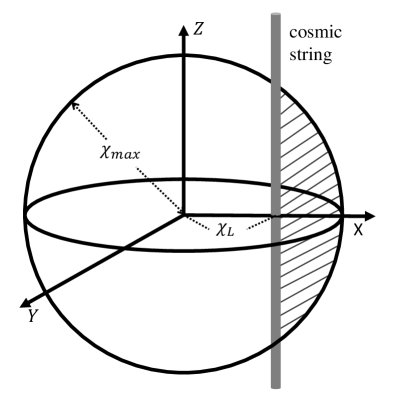
Figure 3: The comoving coordinate system and the placement of a cosmic string used for lensing detection calculation. The hatched region indicates the possible source positions that can give detectable lensing.

The $V_{s}$ is the volume of the hatched region in Fig. 3. The maximum source distance $\chi_{\rm max}$ is determined by the observability of the GW, i.e. SNR $>10$ condition. If a string is put on the $XZ$ plane as in the figure, for each $(X,Z)$ location, there is a maximum $Y_{\rm max}(X,Z)$ that can satisfy detection criteria. Then

$$V_{s}(\chi_{L},\Delta)\,=\,2\iint^{\chi_{\rm max}}Y_{\rm max}(X,Z)\,dXdZ,$$ (26)

where the factor 2 accounts for $Y<0$ and the integration is over the hatched region. $Y_{\rm max}$ is determined by the remaining detection criteria (chi-square test and the frequency resolution).

Just for more technical details, from Eq. (3) and Eq. (7), the two parameters that essentially determine the criteria are $w$ and $y$. So instead of evaluating the criteria in the 3D space of $(X,Y,Z)$, it is easier to integrate over the 2D plane of $(w,y)$. This gives $y_{\rm max}$ as a function of $w$. Thus, for a given $(X,Z)$, we first compute $w$ (note that $Y_{\rm max}\ll X\text{ or }Z$) and then convert $y_{\rm max}(w)$ to $Y_{\rm max}(X,Z)$ by using $y=2\tan^{-1}\left[Y/(X-\chi_{L})\right]/\Delta$. In numerical integration, $X$ and $Z$ axes are divided by 16 sectors with rectangular quadrature, while the Boolean condition $\sqrt{X^{2}+Z^{2}}\leq\chi_{\rm max}$ is imposed. Similarly, $V_{6D}$ integral is done over rectangular quadratures with 16 sectors for $0\leq\chi_{L}\leq\chi_{\rm max}$.

Appendix C Detection rate for each mass bins

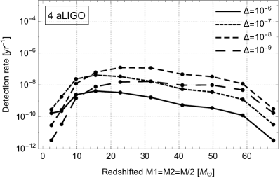
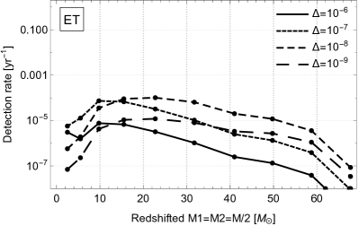
Figure 4: Detection rate of the GW fringe with four aLIGOs (left) and one ET (right) in each binary mass bin. Several values of string tensions $\Delta=8\pi G\mu=10^{-6,-7,-8,-9}$ are shown.

In Fig. 4, we show LIGO-band detection rate of each binary mass bin. First of all, the detection rates typically decrease in both small and large masses. This is because small-mass binaries produce weak GWs, whereas large-mass binaries have low merger-rate densities Belczynski:2016obo ; http://www.syntheticuniverse.org/stvsgwo.html . Secondly, the overall detection rates grow with $\Delta$, except for large $\Delta\simeq 10^{-7}$ – $10^{-6}$. This is in accordance with Sec. 4, but the suppression is more severe for heavy binaries, which spend relatively shorter time in the LIGO-band.

References

- (1) T. W. B. Kibble, “Some Implications of a Cosmological Phase Transition,” Phys. Rept. 67, 183 (1980). doi:10.1016/0370-1573(80)90091-5
- (2) V. Vanchurin, K. D. Olum and A. Vilenkin, “Scaling of cosmic string loops,” Phys. Rev. D 74, 063527 (2006) doi:10.1103/PhysRevD.74.063527 [gr-qc/0511159].
- (3) J. V. Rocha, “Scaling solution for small cosmic string loops,” Phys. Rev. Lett. 100, 071601 (2008) doi:10.1103/PhysRevLett.100.071601 [arXiv:0709.3284 [gr-qc]].
- (4) T. W. B. Kibble, “Topology of cosmic domains and strings,” J. Phys. A 9, 8 (1976) doi:10.1088/0305-4470/9/8/029.
- (5) A. Vilenkin, “Cosmic Strings and Domain Walls,” Phys. Rept. 121, 263 (1985). doi:10.1016/0370-1573(85)90033-X
- (6) D. Harari and P. Sikivie, “The Gravitational Field of a Global String,” Phys. Rev. D 37, 3438 (1988). doi:10.1103/PhysRevD.37.3438
- (7) T. Charnock, A. Avgoustidis, E. J. Copeland and A. Moss, “CMB constraints on cosmic strings and superstrings,” Phys. Rev. D 93, no. 12, 123503 (2016) doi:10.1103/PhysRevD.93.123503 [arXiv:1603.01275 [astro-ph.CO]].
- (8) S. Kuroyanagi, K. Miyamoto, T. Sekiguchi, K. Takahashi and J. Silk, “Forecast constraints on cosmic strings from future CMB, pulsar timing and gravitational wave direct detection experiments,” Phys. Rev. D 87, no. 2, 023522 (2013) Erratum: [Phys. Rev. D 87, no. 6, 069903 (2013)] doi:10.1103/PhysRevD.87.069903, 10.1103/PhysRevD.87.023522 [arXiv:1210.2829 [astro-ph.CO]].
- (9) J. J. Blanco-Pillado, K. D. Olum and X. Siemens, “New limits on cosmic strings from gravitational wave observation,” Phys. Lett. B 778, 392 (2018) doi:10.1016/j.physletb.2018.01.050 [arXiv:1709.02434 [astro-ph.CO]].
- (10) C. Ringeval and T. Suyama, “Stochastic gravitational waves from cosmic string loops in scaling,” JCAP 1712, no. 12, 027 (2017) doi:10.1088/1475-7516/2017/12/027 [arXiv:1709.03845 [astro-ph.CO]].
- (11) B. P. Abbott et al. [LIGO Scientific and Virgo Collaborations], “Constraints on cosmic strings using data from the first Advanced LIGO observing run,” Phys. Rev. D 97, no. 10, 102002 (2018) doi:10.1103/PhysRevD.97.102002 [arXiv:1712.01168 [gr-qc]].
- (12) Y. Cui, M. Lewicki, D. E. Morrissey and J. D. Wells, “Cosmic Archaeology with Gravitational Waves from Cosmic Strings,” Phys. Rev. D 97, no. 12, 123505 (2018) doi:10.1103/PhysRevD.97.123505 [arXiv:1711.03104 [hep-ph]].
- (13) Y. Cui, M. Lewicki, D. E. Morrissey and J. D. Wells, “Probing the pre-BBN universe with gravitational waves from cosmic strings,” arXiv:1808.08968 [hep-ph].
- (14) R. Consiglio, O. Sazhina, G. Longo, M. Sazhin and F. Pezzella, “On the number of cosmic strings,” Mon. Not. Roy. Astron. Soc. 439, no. 4, 3213 (2014) doi:10.1093/mnras/stu048 [arXiv:1112.5186 [astro-ph.CO]].
- (15) D. Harari and P. Sikivie, “On the Evolution of Global Strings in the Early Universe,” Phys. Lett. B 195, 361 (1987). doi:10.1016/0370-2693(87)90032-3
- (16) P. Sikivie, “Cosmic global strings,” Phys. Scripta T 36, 127 (1991). doi:10.1088/0031-8949/1991/T36/014
- (17) A. Vilenkin, “Gravitational Field of Vacuum Domain Walls and Strings,” Phys. Rev. D 23, 852 (1981). doi:10.1103/PhysRevD.23.852
- (18) J. R. Gott, III, “Gravitational lensing effects of vacuum strings: Exact solutions,” Astrophys. J. 288, 422 (1985). doi:10.1086/162808
- (19) C. M. Yoo, R. Saito, Y. Sendouda, K. Takahashi and D. Yamauchi, “Femto-lensing due to a Cosmic String,” PTEP 2013, 013E01 (2013) doi:10.1093/ptep/pts045 [arXiv:1209.0903 [astro-ph.CO]].
- (20) T. Suyama, T. Tanaka and R. Takahashi, “Exact wave propagation in a spacetime with a cosmic string,” Phys. Rev. D 73, 024026 (2006) doi:10.1103/PhysRevD.73.024026 [astro-ph/0512089].
- (21) S. Jung and C. S. Shin, “Gravitational-Wave Fringes at LIGO: Detecting Compact Dark Matter by Gravitational Lensing,” Phys. Rev. Lett. 122, no. 4, 041103 (2019) doi:10.1103/PhysRevLett.122.041103 [arXiv:1712.01396 [astro-ph.CO]].
- (22) T. T. Nakamura, “Gravitational lensing of gravitational waves from inspiraling binaries by a point mass lens,” Phys. Rev. Lett. 80, 1138 (1998). doi:10.1103/PhysRevLett.80.1138
- (23) Schneider, P., Ehlers, J., & Falco, E. E., “Gravitational Lenses,” Springer-Verlag Berlin Heidelberg New York (1992)
- (24) T. Nakamura and S. Deguchi “Wave Optics in Gravitational Lensing,” Prog. Theor. Phys. Suppl. 133, 137 (1999)
- (25) I. Fernández-Núñez and O. Bulashenko, “Emergence of Fresnel diffraction zones in gravitational lensing by a cosmic string,” Phys. Lett. A 381, 1764 (2017) doi:10.1016/j.physleta.2017.03.046 [arXiv:1612.07218 [astro-ph.CO]].
- (26) J. B. Keller, “Geometric theory of diffraction,” J. Opt. Soc. Am. 52, 2 (1962)
- (27) R. R. Caldwell and B. Allen, “Cosmological constraints on cosmic string gravitational radiation,” Phys. Rev. D 45, 3447 (1992). doi:10.1103/PhysRevD.45.3447
- (28) K. J. Mack, D. H. Wesley and L. J. King, “Observing cosmic string loops with gravitational lensing surveys,” Phys. Rev. D 76, 123515 (2007) doi:10.1103/PhysRevD.76.123515 [astro-ph/0702648 [ASTRO-PH]].
- (29) J. J. Blanco-Pillado, K. D. Olum and B. Shlaer, “The number of cosmic string loops,” Phys. Rev. D 89, no. 2, 023512 (2014) doi:10.1103/PhysRevD.89.023512 [arXiv:1309.6637 [astro-ph.CO]].
- (30) A. Vilenkin, “Cosmic strings as gravitational lenses,” Astrophys. J. 282, L51 (1984). doi:10.1086/184303
- (31) L. Dai, S. S. Li, B. Zackay, S. Mao and Y. Lu, “Detecting Lensing-Induced Diffraction in Astrophysical Gravitational Waves,” Phys. Rev. D 98, no. 10, 104029 (2018) doi:10.1103/PhysRevD.98.104029 [arXiv:1810.00003 [gr-qc]].
- (32) P. Christian, S. Vitale and A. Loeb, “Detecting Stellar Lensing of Gravitational Waves with Ground-Based Observatories,” Phys. Rev. D 98, no. 10, 103022 (2018) doi:10.1103/PhysRevD.98.103022 [arXiv:1802.02586 [astro-ph.HE]].
- (33) K. H. Lai, O. A. Hannuksela, A. Herrera-Martín, J. M. Diego, T. Broadhurst and T. G. F. Li, “Discovering intermediate-mass black hole lenses through gravitational wave lensing,” Phys. Rev. D 98, no. 8, 083005 (2018) doi:10.1103/PhysRevD.98.083005 [arXiv:1801.07840 [gr-qc]].
- (34) P. Ajith et al., “Template bank for gravitational waveforms from coalescing binary black holes: Nonspinning binaries,” Phys. Rev. D 77, 104017 (2008) doi:10.1103/PhysRevD.77.104017
- (35) S. Khan et al., “Frequency-domain gravitational waves from nonprecessing black-hole binaries. II. A phenomenological model for the advanced detector era,” Phys. Rev. D 93, 044007 (2016) doi:10.1103/PhysRevD.93.044007
- (36) K. Belczynski, D. E. Holz, T. Bulik and R. O’Shaughnessy, “The first gravitational-wave source from the isolated evolution of two 40-100 Msun stars,” Nature 534, 512 (2016) doi:10.1038/nature18322 [arXiv:1602.04531 [astro-ph.HE]].
- (37) B. P. Abbott et al. [LIGO Scientific and Virgo Collaborations], “GW150914: The Advanced LIGO Detectors in the Era of First Discoveries,” Phys. Rev. Lett. 116, no. 13, 131103 (2016) doi:10.1103/PhysRevLett.116.131103 [arXiv:1602.03838 [gr-qc]].
- (38) D.V. Martynov et al., “Sensitivity of the Advanced LIGO detectors at the beginning of gravitational wave astronomy,” Phys. Rev. D 93, 112004 (2016) doi:10.1103/PhysRevD.93.112004
- (39) The merger rate estimation from Belczynski:2016obo is being updated at: http://www.syntheticuniverse.org/stvsgwo.html
- (40) S. Hild et al., “Sensitivity Studies for Third-Generation Gravitational Wave Observatories,” Class. Quant. Grav. 28, 094013 (2011) doi:10.1088/0264-9381/28/9/094013 [arXiv:1012.0908 [gr-qc]].
- (41) P. W. Graham, J. M. Hogan, M. A. Kasevich and S. Rajendran, “Resonant mode for gravitational wave detectors based on atom interferometry,” Phys. Rev. D 94, no. 10, 104022 (2016) doi:10.1103/PhysRevD.94.104022 [arXiv:1606.01860 [physics.atom-ph]].
- (42) P. W. Graham et al. [MAGIS Collaboration], “Mid-band gravitational wave detection with precision atomic sensors,” arXiv:1711.02225 [astro-ph.IM].
- (43) K. Yagi and N. Seto, “Detector configuration of DECIGO/BBO and identification of cosmological neutron-star binaries,” Phys. Rev. D 83, 044011 (2011) Erratum: [Phys. Rev. D 95, no. 10, 109901 (2017)] doi:10.1103/PhysRevD.95.109901, 10.1103/PhysRevD.83.044011 [arXiv:1101.3940 [astro-ph.CO]].
- (44) http://www.et-gw.eu/index.php/etdsdocument
- (45) A. Klein et al., “Science with the space-based interferometer eLISA: Supermassive black hole binaries,” Phys. Rev. D 93, no. 2, 024003 (2016) doi:10.1103/PhysRevD.93.024003 [arXiv:1511.05581 [gr-qc]].
- (46) R. Takahashi and T. Nakamura, “Wave effects in gravitational lensing of gravitational waves from chirping binaries,” Astrophys. J. 595, 1039 (2003) doi:10.1086/377430 [astro-ph/0305055].
- (47) A. Gould, “Femtolensing of gamma-ray bursters,” Astrophys. J. 386, L5 (1992) doi:10.1086/186279
- (48) A. Barnacka, J. F. Glicenstein and R. Moderski, “New constraints on primordial black holes abundance from femtolensing of gamma-ray bursts,” Phys. Rev. D 86, 043001 (2012) doi:10.1103/PhysRevD.86.043001 [arXiv:1204.2056 [astro-ph.CO]].
- (49) A. Katz, J. Kopp, S. Sibiryakov and W. Xue, “Femtolensing by Dark Matter Revisited,” JCAP 1812, 005 (2018) doi:10.1088/1475-7516/2018/12/005 [arXiv:1807.11495 [astro-ph.CO]].
- (50) S. Jung and T. Kim, “GRB lensing parallax: Closing primordial black hole dark matter mass window,” Phys. Rev. Res. 2, no. 1, 013113 (2020) [Phys. Rev. Research. 2, 013113 (2020)] doi:10.1103/PhysRevResearch.2.013113 [arXiv:1908.00078 [astro-ph.CO]].
- (51) N. Matsunaga and K. Yamamoto, “The finite source size effect and the wave optics in gravitational lensing,” JCAP 0601, 023 (2006) doi:10.1088/1475-7516/2006/01/023 [astro-ph/0601701].
- (52) O. S. Sazhina, M. V. Sazhin, V. N. Sementsov, “Cosmic microwave background anisotropy induced by a moving straight cosmic string,” J. Exp. Theor. Phys. 106, 878 (2008) doi:10.1134/S1063776108050051
- (53) B. Shlaer and S.-H. H. Tye, “Cosmic string lensing and closed time-like curves,” Phys. Rev. D 72, 043532 (2005) doi:10.1103/PhysRevD.72.043532 [hep-th/0502242].
- (54) B. P. Abbott et al. [LIGO Scientific and Virgo Collaborations], “Tests of general relativity with GW150914,” Phys. Rev. Lett. 116, no. 22, 221101 (2016) Erratum: [Phys. Rev. Lett. 121, no. 12, 129902 (2018)] doi:10.1103/PhysRevLett.116.221101, 10.1103/PhysRevLett.121.129902 [arXiv:1602.03841 [gr-qc]].
- (55) R. Takahashi and T. Nakamura, “Deci hertz laser interferometer can determine the position of the coalescing binary neutron stars within an arc minute a week before the final merging event to black hole,” Astrophys. J. 596, L231 (2003) doi:10.1086/379112 [astro-ph/0307390].
- (56) P. W. Graham and S. Jung, “Localizing Gravitational Wave Sources with Single-Baseline Atom Interferometers,” Phys. Rev. D 97, no. 2, 024052 (2018) doi:10.1103/PhysRevD.97.024052 [arXiv:1710.03269 [gr-qc]].
- (57) S. Isoyama, H. Nakano and T. Nakamura, “Multiband Gravitational-Wave Astronomy: Observing binary inspirals with a decihertz detector, B-DECIGO,” PTEP 2018, no. 7, 073E01 (2018) doi:10.1093/ptep/pty078 [arXiv:1802.06977 [gr-qc]].
- (58) R. Nair and T. Tanaka, “Synergy between ground and space based gravitational wave detectors. Part II: Localisation,” JCAP 1808, no. 08, 033 (2018) doi:10.1088/1475-7516/2018/08/033 [arXiv:1805.08070 [gr-qc]].
- (59) H. G. Choi and S. Jung, “New probe of dark matter-induced fifth force with neutron star inspirals,” Phys. Rev. D 99, no. 1, 015013 (2019) doi:10.1103/PhysRevD.99.015013 [arXiv:1810.01421 [hep-ph]].